Unsupervised Domain Expansion for Visual Categorization

Abstract.

Expanding visual categorization into a novel domain without the need of extra annotation has been a long-term interest for multimedia intelligence. Previously, this challenge has been approached by unsupervised domain adaptation (UDA). Given labeled data from a source domain and unlabeled data from a target domain, UDA seeks for a deep representation that is both discriminative and domain-invariant. While UDA focuses on the target domain, we argue that the performance on both source and target domains matters, as in practice which domain a test example comes from is unknown. In this paper we extend UDA by proposing a new task called unsupervised domain expansion (UDE), which aims to adapt a deep model for the target domain with its unlabeled data, meanwhile maintaining the model’s performance on the source domain. We propose Knowledge Distillation Domain Expansion (KDDE) as a general method for the UDE task. Its domain-adaptation module can be instantiated with any existing model. We develop a knowledge distillation based learning mechanism, enabling KDDE to optimize a single objective wherein the source and target domains are equally treated. Extensive experiments on two major benchmarks, i.e., Office-Home and DomainNet, show that KDDE compares favorably against four competitive baselines, i.e., DDC, DANN, DAAN, and CDAN, for both UDA and UDE tasks. Our study also reveals that the current UDA models improve their performance on the target domain at the cost of noticeable performance loss on the source domain.

1. Introduction

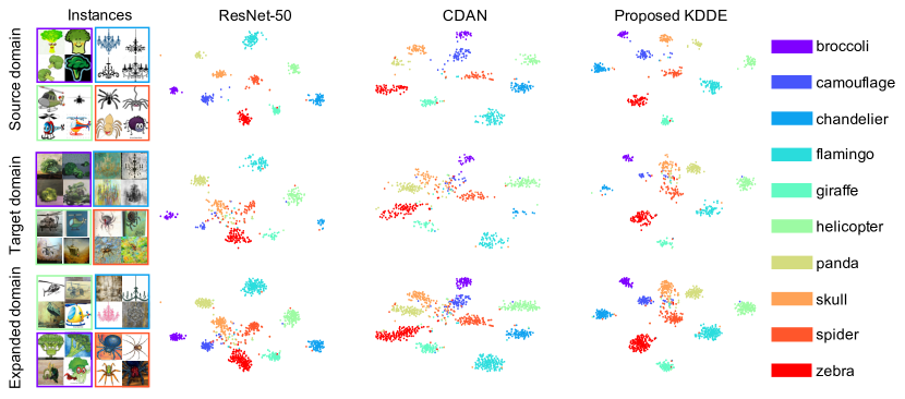
Figure 1. Visualization of deep feature spaces obtained by three models, that is, ResNet-50 fully trained on a labeled source domain, CDAN (Long et al., 2018) as a state-of-the-art domain adaptation model and the proposed Knowledge Distillation Domain Expansion (KDDE) that adaptively learns from both ResNet-50 and CDAN. Across the source, target and expanded domains, intra-class data points tend to stay closer while inter-class data points are more distant in the feature space of KDDE. With no need of extra labeled data, KDDE effectively expands the applicable domain of visual classifiers.

It has been recognized early by the multimedia community that visual classifiers trained on a specific domain do not necessarily perform well on a distinct domain (Yang et al., 2007; Jiang et al., 2008; Duan et al., 2009). Even for the same concept, e.g., helicopter, changing from one domain to another, e.g., clipart $\rightarrow$ painting, would result in significant discrepancy in visual appearance, see Fig. 1. When such discrepancy is propagated to the feature space wherein classification is performed, performance degeneration occurs. Note that the advance of deep learning does not alleviate the problem. Rather, due to its “super” learning ability, deep representations tend to be dataset biased (Zhang et al., 2018a).

In order to improve the generalization ability of a deep visual classifier without the need of extra annotation, deep unsupervised domain adaptation (UDA) has been actively studied (Tzeng et al., 2014; Sun and Saenko, 2016; Long et al., 2018; Li et al., 2019). Given the availability of labeled data from a source domain and unlabeled data from a target domain, UDA seeks for a deep representation that is both discriminative and domain-invariant. In the seminal work by Tzeng et al.  (Tzeng et al., 2014), a deep convolutional neural network termed Deep Domain Confusion (DDC) is developed to simultaneously minimize the classification loss and a domain discrepancy loss computed in terms of first-order statistics of the deep features from the two domains. Follow-ups improve DDC in varied aspects, including Deep CORAL (Sun and Saenko, 2016) that replaces first-order statistics by second-order statistics, JAN (Long et al., 2017) that measures domain discrepancy on multiple task-specific layers, and DANN (Ganin et al., 2016) and CDAN (Long et al., 2018) that reduce domain discrepancy by adversarial learning, to name just a few.

While the above efforts have accomplished well for the UDA task, how they perform in the original source domain is mostly unreported, to the best of our knowledge. The absence of performance evaluation on the source domain rises an important question: is a domain-adapted model indeed domain-invariant? A follow-up question is whether the performance gain for the target domain is obtained at the cost of significant performance loss in the source domain? These two questions are so far overlooked, as existing works on UDA typically assume to know which is the target distribution to tackle. In synthetic-to-real UDA (Zou et al., 2018; Toldo et al., 2020), for instance, one treats the synthetic data as the source domain and thus only the real dataset performance matters in the end. However, we argue that the performance on both source and target domains matters, as in practice which domain a test example comes from can be unknown. In this paper we extend UDA by proposing a new task, which aims to adapt a deep model for the target domain with its unlabeled data, meanwhile maintaining the model’s performance on the source domain. As this factually expands the model’s applicable domain, we coin the new task unsupervised domain expansion (UDE).

UDE targets at an expanded domain consisting of test examples from the source and target domains both. So it handles with ease the situation when the domain of a test example is unknown. Such a situation is not uncommon. Consider the medical field for instance. Optical Coherence Tomography (OCT) images, as an important means for ophthalmologists to assess retinal conditions, are actively used for automated retinal screening and referral recommendation (De Fauw et al., 2018; Kermany et al., 2018; Wang et al., 2019c). As a matter of fact, an eye center is often equipped with multiple types of OCT devices made by distinct manufacturers, let alone multiple eye centers. Meanwhile, OCT images taken by distinct devices can show noticeable discrepancy in their visual appearance, see Fig. 2. Even though UDA improves the generalization ability of a model trained on samples collected from one device for another device, domain adaptation per device is economically unaffordable. With the goal to optimize performance for the expanded domain with a single model, UDE is essential for real-world medical image classification. What is more, by simultaneously evaluating on both source and target domains, UDE provides a direct measure of to what extent a resultant model is domain-invariant, which is mostly missing in the rich literature of UDA.

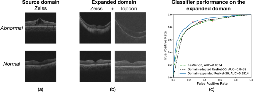
Figure 2. Abnormal OCT image recognition as a showcase of Unsupervised Domain Expansion (UDE). OCT images taken by distinct devices, e.g., (a) Zeiss Cirrus OCT and (b) Topcon 2000FA OCT, often differ noticeably in their visual appearance. A domain-adapted classifier, departing from the source domain (Zeiss), emphasizes its performance on the target domain (Topcon). In contrast, a domain-expanded classifier aims for the overall performance of both source and target domains, which is essential for real-world applications. Red circles on (c) ROC curves of the three classifiers indicate their operating points using the default cutoff of 0.5. See Section 4 for detailed experiments.

Although UDA models have considered the performance of the source domain in their learning process, the two objectives to be optimized, i.e., discriminability and domain-invariance, are not always consistent. Such a property makes the existing models difficult to maximize their performance on the expanded source + target domain. While existing models such as DDC and CDAN have a trade-off parameter to balance the two objectives, tunning such a parameter was among our early yet unsuccessful efforts, see Section 4.6.4. A new method for UDE is thus in demand.

A straightforward solution for the UDE task is to train a domain classifier to automatically determine which domain a specific test image belongs to. Accordingly, if the test image is deemed to be from the source (or target) domain, a model trained on the source domain (or another model adapted w.r.t. the target domain) is selected to handle the image, see Fig. 3 (a). Such a solution is cumbersome as it needs to deploy three classifiers at the inference stage. Moreover, misclassification by the domain classifier will make the test image assigned to an inappropriate model. By contrast, we aim for a single domain-expanded model that handle test images from both domains in an unbiased manner, as illustrated in Fig. 3 (b). To that end, we resort to deep knowledge distillation (KD) (Hinton et al., 2015), initially developed for transferring “dark” knowledge in a cumbersome deep model to a smaller model. We exploit the KD technique with a novel motivation of simultaneously transferring knowledge from the source and domain-adapted models into another model to make that specific model effective for the expanded domain.

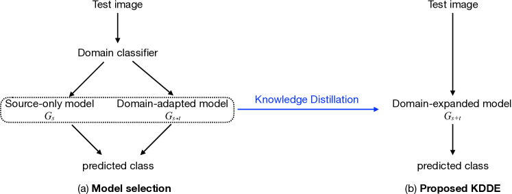
Figure 3. Conceptual illustration of two solutions for UDE. (a) Model selection: A straightforward solution that deploys a source-only model $G_{s}$ for the source domain and a domain-adapted model $G_{s\rightarrow t}$ for the target domain, and then chooses which one to use conditioned on the output of a domain classifier. (b) Our solution: Develop a single yet domain-expanded model $G_{s+t}$ by distilling dark knowledge from both $G_{s}$ and $G_{s\rightarrow t}$.

In sum, our contributions are as follows:

• We propose UDE as a new task. By simultaneously considering the performance on the source and target domains, UDE is more practical yet more challenging than UDA. The new task allows us to directly measure to what extent a model is domain-invariant. Moreover, to the best of our knowledge, this paper is the first to systematically document the performance of the current UDA models on the source domain, empirically revealing that they are essentially domain-specific rather than domain-invariant.

• We propose Knowledge Distillation Domain Expansion (KDDE), a general method for the UDE task. Its domain-adaptation module can be instantiated with any existing model. Moreover, our knowledge distillation based learning mechanism allows KDDE to optimize a single objective wherein the source and target domains are equally treated. Note that the knowledge distillation technique used by this paper is not new by itself. We adopt it as a proof-of-concept solution for UDE, developed based on a teacher-student framework. While built upon existing components, KDDE provides a principled approach to leveraging previous UDA models for domain expansion, even when multi-domain shifts exist.

• Extensive experiments on two major benchmarks, i.e., Office-Home (Venkateswara et al., 2017) and DomainNet (Peng et al., 2019), show that KDDE outperforms four competitive baselines, i.e., DDC, DANN, DAAN, and CDAN, for the UDA and UDE tasks both. Besides, experiments on cross-device OCT image classification show a high potential of the proposed method for improving the generalization ability of a medical image classification system in a real-world multi-device scenario.

2. Related Work

As we have noted in Section 1, prior work on UDE does not exist. Nonetheless, UDE relies on UDA techniques (Tzeng et al., 2014; Ganin et al., 2016; Long et al., 2018; Li et al., 2019; Long et al., 2017; Sun and Saenko, 2016). The proposed KDDE model also benefits from progress in knowledge distillation based deep transfer learning (Hinton et al., 2015; Romero et al., 2015; Zhang et al., 2018b; Zhang et al., 2019b). Therefore, we review briefly recent developments regarding the two topics.

2.1. Deep Unsupervised Domain Adaptation

Depending on how domain discrepancy is modeled, we categorize deep learning methods for UDA into two categories, i.e., metric-based methods (Tzeng et al., 2014; Long et al., 2015, 2017; Sun and Saenko, 2016; Peng et al., 2019; Kang et al., 2019) and adversarial methods (Ganin et al., 2016; Tzeng et al., 2017; Yu et al., 2019; Long et al., 2018; Li et al., 2019). As a representative work of the first category, DDC (Tzeng et al., 2014) measures domain discrepancy in terms of the Euclidean distance between mean feature vectors of the source and target domains. By jointly minimizing the classification loss on the labeled source domain and the inter-domain distance, DDC aims to learn discriminative yet domain-invariant feature representations. While DDC considers only the last feature layer of the underlying classification network, Joint Adaptation Network (JAN) (Long et al., 2017) measures domain discrepancy on multiple task-specific layers. Deep CORAL (Sun and Saenko, 2016) utilizes second-order statistics, learning to reduce the divergence between the covariance matrices of the two domains. Although the above models are end-to-end, their metrics for domain discrepancy have to be empirically predefined, which could be suboptimal.

To bypass the difficulty in specifying a proper discrepancy metric, several methods that resort to adversarial learning have been developed (Ganin et al., 2016; Long et al., 2018; Saito et al., 2018; Yu et al., 2019; Li et al., 2019). Domain Adversarial Neural Network (DANN) (Ganin et al., 2016) introduces a domain classifier as a discriminator, while its feature extractor tries to generate domain-invariant features to confuse the discriminator. Dynamic Adversarial Adaptation (DAAN) (Yu et al., 2019) improves DANN by introducing multiple concept-specific discriminators to dynamically weigh the importance of marginal and conditional distributions. In order to align both learned features and predicted classes, Conditional Discriminative Adversarial Network (CDAN) (Long et al., 2018) extends DANN by taking multilinear conditioning of feature representations and classification results as the input of its discriminator. Different from CDAN that uses a feed-forward network as its discriminator, Maximum Classifier Discrepancy (MCD) (Saito et al., 2018) builds a CNN network with two classification branches, and exploits the discrepancy between their output to determine whether a given example is from the source or target domain. Joint Adversarial Domain Adaptation (JADA) (Li et al., 2019) extends MCD by adding an additional domain classifier to achieve class-wise and domain-wise alignments. While all the above works concentrate on the target domain, our work provides a generic approach to improving their performance on the expanded domain.

2.2. Deep Knowledge Distillation

Deep knowledge distillation is originally proposed to transfer “dark” knowledge in a cumbersome deep model or an ensemble to a smaller model (Hinton et al., 2015). Compared with the big model, the small model trained by its own typically has a lower accuracy. Knowledge distillation provides a principled mechanism to let the small model learn as a student from the big model as a teacher. In particular, the student mimics the teacher’s behavior by minimizing the Kullback-Leibler divergence or the cross-entropy loss between the output of the two models (Hinton et al., 2015; Zhang et al., 2018b). For its general applicability, knowledge distillation has been widely used in varied tasks such as object detection (Chen et al., 2017), pose regression (Saputra et al., 2019), semantic segmentation (Liu et al., 2019), and saliency prediction (Zhang et al., 2019b). Not surprisingly, the technology has been investigated for domain adaptation in the context of speech recognition (Asami et al., 2017; Meng et al., 2018, 2019) and image recongition (French and Fisher, 2018; Yang Zou, 2019). As we target at domain expansion, we leverage knowledge distillation in a different manner, both conceptually and technically.

3. Our Method

3.1. Problem Formalization

We consider multi-class visual categorization, where a specific example $x$ belongs to one of $k$ predefined visual concepts. Ground truth of $x$ is indicated by $y$, a $k$-dimensional one-hot vector. A deep visual classification network $G$ classifies $x$ by first employing a feature extractor $F$ to obtain a vectorized feature representation $z$ from its raw pixels. Then, $z$ is fed into a $k$-way classifier $C$ to produce a categorical probability vector $\hat{y}$, where the value of its $i$-th dimension is the probability of the example belonging to the $i$-th concept, i.e.,

(1) $$\left\{\begin{array}[]{lll}z&=&F(x),\\ \hat{y}&=&C(z).\end{array}\right.$$

Such a paradigm as expressed in Eq. 1 remains valid to this day, even though $F$ and $C$ have now been jointly deployed and end-to-end trained by deep learning.

As UDE is derived from UDA, we adopt common notations from the latter for the ease of consistent description. For both UDE and UDA, we have access to a set of $n_{s}$ labeled training examples $\{(x_{s,i},y_{s,i})\}_{i=1}^{n_{s}}$ from a source domain $D_{s}$ and a set of $n_{t}$ unlabeled training examples $\{x_{t,i}\}_{i=1}^{n_{t}}$ from a target domain $D_{t}$. However, different from UDA that focuses on $D_{t}$, UDE treats the expanded domain $D_{s}+D_{t}$ as its “target” domain. Therefore, our goal is to train a unified model that can accurately classify novel examples regardless of their original domains.

3.2. UDE by Knowledge Distillation

We propose a knowledge distillation based method for UDE, which we term KDDE. As illustrated in Fig. 4, KDDE is performed in two steps. In the first step, two domain-specific classifiers, denoted as $G_{s}$ and $G_{s\rightarrow t}$, are trained for the source and target domains, respectively. Note that we use the notation $s\rightarrow t$ to emphasize that as $D_{t}$ is unlabeled, any domain-adapted classifier shall departure from $D_{s}$. In the second step, we treat $G_{s}$ and $G_{s\rightarrow t}$ as two teacher models and transfer their “dark” knowledge into a student model $G_{s+t}$ via a knowledge distillation process. In particular, by mimicking $G_{s}$ for classifying examples from $D_{s}$ and $G_{s\rightarrow t}$ for $D_{t}$, $G_{s+t}$ essentially becomes domain-invariant. We detail the two steps as follows.

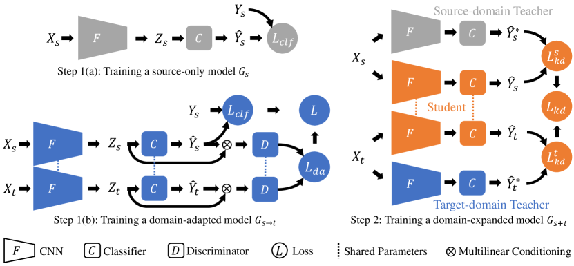
Figure 4. Conceptual diagram of the proposed KDDE method for UDE. KDDE is run in two steps. First, a model $G_{s}$ is trained on the labeled source domain by standard supervised learning, while another model $G_{s\rightarrow t}$ for the unlabeled target domain is trained by unsupervised domain adaptation (here CDAN (Long et al., 2018) as a running example). Then, knowledge distillation is performed to transfer “dark” knowledge from the two domain-specific models into a student model $G_{s+t}$ to make it applicable to both domains.

3.2.1. Step 1(a): Training a source-only model $G_{s}$

Learning a classifier from labeled data is relatively simple. We adopt the cross-entropy loss, a common classification loss used for training a multi-class deep neural network. Given $(X_{s},Y_{s})$ as $\{(x_{s,i},y_{s,i})\}_{i=1}^{n_{s}}$, the classification loss is written as

(2) $$L_{clf}(X_{s},Y_{s},G)=\frac{1}{n_{s}}\sum_{(x_{s},y_{s})\in(X_{s},Y_{s})}y_{s}\log(G(x_{s})).$$

By minimizing $L_{clf}(X_{s},Y_{s},G)$, we obtain a domain-specific model for $D_{s}$ as

(3) $$G_{s}=\arg\underset{G}{\min}\;L_{clf}(X_{s},Y_{s},G).$$

3.2.2. Step 1(b): Training a domain-adapted model $G_{s\rightarrow t}$

Recall that KDDE, as a two-stage solution, is agnostic to the implementation of a specific UDA model used in its first stage. Hence, for obtaining $G_{s\rightarrow t}$, any method for unsupervised domain adaptation can, in principle, be adopted. A typical process of model adaptation tries to strike a proper balance between a model’s discriminability, as reflected by the classification loss on $D_{s}$, and its domain-invariant representation ability, as measured by inter-domain discrepancy between $D_{s}$ and $D_{t}$. More formally, we have

(4) $$G_{s\rightarrow t}=\arg\underset{G}{\min}\;\underbrace{L_{clf}(X_{s},Y_{s},G)}_{\mbox{discriminative}}+\lambda\cdot\underbrace{L_{da}(X_{s},X_{t},G)}_{\mbox{domain-invariant}},$$

where $L_{da}$ is a domain discrepancy based loss, and $\lambda$ is a positive hyper-parameter. Algorithm 1 describes the domain adaptation process at a high level. In what follows, we use the state-of-the-art CDAN model (Long et al., 2018) as a running example to instantiate $L_{da}$.

Input: $(X_{s},Y_{s})$, $X_{t}$

Output: $G_{s\rightarrow t}$

1 Set hyper-parameters: $\lambda,MAX\_EPOCHS,BATCH\_SIZE$;

2 Compute the number of iterations per epoch $MAX\_ITERS$, given $|X_{s}|$ and $BATCH\_SIZE$;

3 Initialize $G_{s\rightarrow t}$ with an ImageNet-pretrained model;

4 for $i\leftarrow 1,\ldots,MAX\_EPOCHS$ do

5       for $j\leftarrow 1,\ldots,MAX\_ITERS$ do

6             Sample a mini-batch $(X_{s,j},Y_{s,j})$ from $(X_{s},Y_{s})$;

7             Sample a mini-batch $X_{t,j}$ from $X_{t}$;

8             Compute the classification loss $L_{clf}(X_{s,j},Y_{s,j},G_{s\rightarrow t})$ ;

9             Compute the inter-domain discrepancy $L_{da}(X_{s,j},X_{t,j},G_{s\rightarrow t})$ ;

10             Update $G_{s\rightarrow t}$ by back propagation based on $L_{clf}+\lambda*L_{da}$

11       end for

12      

13 end for

Algorithm 1 Training a domain-adapted model $G_{s\rightarrow t}$

CDAN reduces domain discrepancy by adversarial learning, where a feed-forward neural network is used as a discriminator $D$ to disentangle the source examples $X_{s}$ from the target examples $X_{t}$. Different from previous adversarial learning based methods where only the intermediate features $F(x_{s})$ and $F(x_{t})$ are considered, CDAN uses multilinear conditioning of the features and class prediction $F(x)\otimes\hat{y}$ as the input of $D$. The output of $D$ is the probability of a given example coming from the source domain. Accordingly, we have the discriminator reward $R$ as

(5) $$R(X_{s},X_{t},G,D)=\sum_{x_{s}\in X_{s}}\log D(F(x_{s})\otimes\hat{y}_{s})+\sum_{x_{t}\in X_{t}}\log(1-D(F(x_{t})\otimes\hat{y}_{t}))$$

The training process of CDAN is implemented as a two-player minimax game as follows:

(6) $$(G_{s\rightarrow t},D)=\arg\underset{G}{\min}\;\underset{D}{\max}\;L_{clf}(X_{s},Y_{s},G)+\lambda\cdot R(X_{s},X_{t},G,D).$$

3.2.3. Step 2. Training a domain-expanded model $G_{s+t}$

Given the domain-specific models $G_{s}$ and $G_{s\rightarrow t}$, we now transfer their capabilities in their own domains into a new model $G_{s+t}$ by knowledge distillation.

In a standard scenario where one wants to distill the knowledge in a big teacher model into a relatively small student model (Hinton et al., 2015), both ground-truth hard labels and soft labels predicted by the teacher model are available for computing the distillation loss. By contrast, in the setting of UDE, the expanded domain has only partial ground-truth labels by definition. More importantly, in order to make $G_{s+t}$ domain-invariant, we shall not only treat $G_{s}$ and $G_{s\rightarrow t}$ equally, but also exploit training examples from $D_{s}$ and $D_{s\rightarrow t}$ in the same manner. To that end, we opt to compute the distillation loss fully based on the soft labels.

Specifically, we adopt the Kullback-Leibler (KL) divergence, as previously used to quantify how a student’s output matches with its teacher (Hinton et al., 2015; Zhang et al., 2018b). Per training example, the soft labels produced by the teacher / student model is essentially a probability distribution over the $k$ concepts. The KL divergence provides a natural measure of how the probability distribution produced by the student is different from that of the teacher, making it a popular loss for knowledge distillation (Hinton et al., 2015; Zhang et al., 2018b; Mirzadeh et al., 2020; Tian et al., 2020; Goldblum et al., 2020; Zhang et al., 2019a; Shi et al., 2019). Indeed, our ablation study in Section 4.6.1 shows that the KL divergence loss is better than other losses such as cross-entroy and $l_{2}$. Let $P(G(X))$ be a $k$-dimensional categorical distribution estimated based on soft labels of an example set $X$ produced by a specific network $G$. Accordingly, the KL divergence from $G$ to each of the two teachers is defined as $KL(P(G_{s}(X_{s}))||P(G(X_{s})))$ and $KL(P(G_{s\rightarrow t}(X_{t}))||P(G(X_{t})))$, respectively. The knowledge distillation loss $L_{kd}$ is defined as

(7) $$L_{kd}(X_{s},X_{t},G_{s},G_{s\rightarrow t},G)=KL(P(G_{s}(X_{s}))||P(G(X_{s})))+KL(P(G_{s\rightarrow t}(X_{t}))||P(G(X_{t}))).$$

Note that the $KL$ terms in Eq. 7 are practically computed by a mini-batch approach. As demonstrated in Fig. 4, in each iteration two mini-batches are independently and randomly sampled from $D_{s}$ and $D_{t}$. They are then fed into $G_{s}$ and $G_{s\rightarrow t}$ to get the soft labels, which are used to approximate $P(G_{s}(X_{s}))$ and $P(G_{s\rightarrow t}(X_{t}))$, respectively. Meanwhile, the two batches are also fed to the student model. Minimizing $L_{kd}$ lets the student model mimic the teachers’ behaviors on both $D_{s}$ and $D_{t}$. Consequently, we obtain the domain-invariant model as

(8) $$G_{s+t}=\arg\underset{G}{\min}\;L_{kd}(X_{s},X_{t},G_{s},G_{s\rightarrow t},G).$$

A high-level description of the training process is given in Algorithm 2. Note that during training, we need to store three models (two teachers $G_{s}$ and $G_{s\rightarrow t}$ and one student $G_{s+t}$). We consider such storage overhead affordable as one typically has access to more computational resources in the training stage than in the inference stage. Moreover, as the teachers are only used to product the soft labels, their weights are frozen, meaning the GPU footprint is much less than simultaneously training all the three models. Also note that in the inference stage. $G_{s+t}$ has the same model size and computation overhead as its teachers. Hence, the proposed method is feasible in real-world scenarios.

Input: $X_{s},X_{t},G_{s},G_{s\rightarrow t}$

Output: $G_{s+t}$

1 Set hyper-parameters: $MAX\_EPOCHS,BATCH\_SIZE$;

2 Compute $MAX\_ITERS$ given $max(|X_{s}|,|X_{t}|)$ and $BATCH\_SIZE$;

3 Initialize $G_{s+t}$ with an ImageNet-pretrained model;

4 for $i\leftarrow 1,MAX\_EPOCH$ do

5       for $j\leftarrow 1,MAX\_ITER$ do

6             Sample $X_{s,j}$ from $X_{s}$;

7             Sample $X_{t,j}$ from $X_{t}$;

8             Compute $L_{kd}(X_{s,j},X_{t,j},G_{s},G_{s\rightarrow t},G_{s+t})$ using Eq. 7;

9             Update $G_{s+t}$ by back propagation based on $L_{kd}$;

10            

11       end for

12      

13 end for

Algorithm 2 Training a domain-expanded model $G_{s+t}$ by KDDE

3.3. Theoretical Analysis

Comparing Eq. 4 and Eq. 8, we see that UDA essentially tries to simultaneously optimize two distinct and sometimes conflictive objectives, i.e., discriminability and domain-invariance. By contrast, our KDDE optimizes a single objective. We believe such a property improves the cross-domain generalization ability of KDDE. Nonetheless, because $G_{s+t}$ is learned from the source model $G_{s}$ and the domain-adapted model $G_{s\rightarrow t}$ in an unbiased manner, domain expansion is obtained at the cost of certain performance drop in the source domain. In other words, $G_{s+t}$ will be less effective than its teacher $G_{s}$ on the source domain, but perform better on the expanded domain, which is the goal of this research.

As for the target domain, $G_{s+t}$ will be better than its teacher $G_{s\rightarrow t}$. According to Ben-David et al. (Ben-David et al., 2007), the target domain error of a UDA model is bounded mainly by its classification error in the source domain and the divergence between the induced source marginal and the induced target marginal. In theory, a UDA model shall be trained to simultaneously minimize the two terms and reduce accordingly the up bound of the target domain error. In practice, however, the classification error in the source domain is not effectively reduced when compared to the source-only model. This is confirmed by our experiments in Section 4 that a number of present-day UDA models including DDC (Tzeng et al., 2014), DANN (Ganin et al., 2016), DAAN (Yu et al., 2019) and CDAN (Long et al., 2018) suffer performance loss in the source domain. With knowledge distillation, $G_{s+t}$ effectively integrates the merits of $G_{s\rightarrow t}$ for minimizing the domain divergence and $G_{s}$ for minimizing the source error, and thus lowers the up bound of the target domain error.

Through knowledge distillation, KDDE injects the dark knowledge of the source-only model $G_{s}$, which performs well on the source domain, and the domain-adapted model $G_{s\rightarrow t}$, which is supposed to perform well on the target domain, into a single model $G_{s+t}$. The effect of knowledge distillation on $G_{s+t}$ is visualized in Fig. 5. By contrast, although CDAN also uses one classifier for both domains, the classifier is essentially $G_{s\rightarrow t}$ used in KDDE. Hence, it is less effective than $G_{s+t}$ to handle the expanded domain. Also notice that the purpose of knowledge distillation is not to reduce the difference between the two teacher models, see Eq. 7. Therefore, KDDE is conceptually different from Maximum classifier discrepancy (MCD) (Saito et al., 2018), which is to reduce the discrepancy between two domain-adapted classifiers via a novel adversarial learning mechanism.

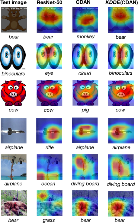
Figure 5. Grad-CAM heatmaps of ResNet-50, CDAN and KDDE. Heatmaps highlight regions important for a model to make predictions. Test images in the first three rows are from the source domain (clipart), while images in the last three rows are from the target domain (real). Activated regions of KDDE ($G_{s+t}$) match well with those of ResNet-50 ($G_{s}$) on the source domain and those of CDAN ($G_{s\rightarrow t}$) on the target domain, suggesting the ability of KDDE to adaptively learn from the two domain-specific models. Data from DomainNet.

4. Experiments

4.1. Datasets

We evaluate the effectiveness of the proposed KDDE model on two public benchmarks, i.e., Office-Home (Venkateswara et al., 2017) and DomainNet (Peng et al., 2019), and a private dataset OCT-11k.

4.1.1. Office-Home

The Office-Home dataset contains 15,588 images of 65 object categories typically found in office and home settings, e.g., chair, table, and TV. Images were collected from the following four distinct domains, i.e., Art (A), Clipart (C), Product (P) and Real world (R). As the dataset is previously used in the domain adaption setting (Long et al., 2018; Wang et al., 2019a; Pinheiro, 2018; Wang et al., 2019b) that considers only performance on the target domain, no test set is provided for the source domain. So to evaluate UDE, for each domain, we randomly divide its images into two disjoint subsets, one for training and the other for test, at a ratio of 1:1, see Table 1. An expanded domain of C+P means using Clipart as the (labeled) source domain, which is expanded with Product as the (unlabeled) target domain. Due to such asymmetric nature of the label information, P+C differs from C+P. Pairing the individual domains results in 12 distinct UDE tasks in total.

Table 1. Three datasets used in our experiments for UDA and UDE. Note that different from the traditional setting of UDA which uses all examples in the source domain for training, the setting of UDE divides the source examples into two disjoint parts, training and test. This allows us to evaluate both UDA and UDE models on the original source domain, which is fully ignored by the literature of UDA.

Dataset	Domains	Images
		total	training	test
Office-Home (Venkateswara et al., 2017) 15,588 images 65 classes	A: Art	2,427	1,201	1,226
	C: Clipart	4,365	2,165	2,200
	P: Product	4,439	2,201	2,238
	R: Real_world	4,357	2,161	2,196
Subset of DomainNet (Peng et al., 2019) 362,470 images 345 classes	c: clipart	48,129	33,525	14,604
	p: painting	72,266	50,416	21,850
	r: real	172,947	120,906	52,041
	s: sketch	69,128	48,212	20,916
OCT-11k (our private dataset) 11,800 images, 2 classes	Z: Zeiss	5,900	5,000	900
	T: Topcon	5,900	5,000	900

4.1.2. DomainNet

DomainNet is a recent large-scale benchmark dataset used in the Visual Domain Adaptation Challenge at ICCV 2019. Compared with Office-Home, DomainNet contains a much larger number of 345 object categories with more intra-class diversity and inter-class ambiguity in visual appearance. As such, it is difficult to obtain high classification accuracy even within a narrow domain. The full set of DomainNet has six domains, i.e., , clipart (c), infograph (i), painting (p), quickdraw (q), real (r) and sketch (s). Saito et al.  (Saito et al., 2019) exclude inforgraph and quickdraw from their study as they find annotations of these two domains are over noisy. We follow their setup, experimenting with the four other domains.

4.1.3. OCT-11k

In order to evaluate the effectiveness of our proposed method for medical image classification in a cross-device setting, we build a set of 11,800 OCT B-scan images, half of which was collected by Zeiss Cirrus OCT and the other half from Topcon 2000FA OCT. All the Zeiss images and a subset of 900 Topcon images were labeled by experts into two classes, namely positive and negative. An image was labeled as positive if certain pathological anomaly such as macular edema, macular hole, drusen, and choroidal atrophy is present. Accordingly, we treat Zeiss as the source domain and Topcon as the target domain. To let the expanded domain contain an equal number of test examples from the individual domains, we randomly sample a subset of 900 Zeiss images as the test set of the source domain. The Zeiss test set contains 581 positives and 319 negatives, while the Topcon test set contains 471 positives and 429 negatives.

4.2. Implementation

4.2.1. Baselines

We compare with the following state-of-the-art domain adaptation models.

• DDC (Tzeng et al., 2014): A classical deep domain adaptation model that minimizes domain discrepancy measured in light of first-order statistics of the deep features.

• DANN (Ganin et al., 2016): Among the first to obtain domain-invariant deep features by adversarial learning.

• DAAN (Yu et al., 2019): An adversarial learning based domain adaptation model, with discriminator networks per concept. For its high demand for GPU memory, we are unable to run DAAN on DomainNet.

• CDAN (Long et al., 2018): Also based adversarial learning, using multilinear conditioning of deep features and classification results as the input of its discriminator.

Recall that DDC and CDAN are representatives for metric-based and adversarial methods, respectively. Hence, we instantiate $G_{s\rightarrow t}$ using the two models separately, resulting in two variants of KDDE, denoted as KDDE(DDC) and KDDE(CDAN).

We implement the source model $G_{s}$ using ResNet-50 that is trained exclusively on the source domain. A model for UDA / UDE shall outperform this baseline on the target / expanded domain. For fair comparison between distinct models, we also use ResNet-50 as their backbones.

4.2.2. Model training

We run all experiments with PyTorch (Paszke et al., 2019). We start with ResNet-50 pre-trained on ImageNet. SGD is used for training, with momentum of $0.9$ and weight decay of $0.0005$. The initial learning rate of ResNet-50, DDC, DANN, DAAN and CDAN is empirically set to $0.001$, and $0.005$ for KDDE. For the adversarial methods, i.e., DANN, DAAN and CDAN, we adopt the inverse-decay learning rate strategy from (Long et al., 2018). As for ResNet-50, DDC and KDDE, the learning rate is decayed by $0.1$ every $30$ epochs on Office-Home and every $10$ epochs on DomainNet, as the latter has much more training examples and thus more iterations per epoch. For the same reason, for each model we train 100 epochs on Office-Home and a less number of 30 epochs on DomainNet.

For DDC, DANN and DAAN, the trade-off parameter $\lambda$ is empirically set to be $10$, $1$, and $1$, respectively. As for CDAN, we follow the original paper (Long et al., 2018) to adjust $\lambda$ dynamically.

4.2.3. Evaluation protocol

For overall performance, we report accuracy, i.e., the percentage of test images correctly classified, as commonly used for evaluating multi-class image classification. For an expanded domain, e.g., A+C, its test set is the union of the test sets of the Art and Clipart domains. To cancel out data imbalance, the accuracy of the expanded domain is obtained by averaging over the two individual domains. The performance of a specific concept is measured by F1-score, the harmonic mean of precision and recall. For binary classification on OCT-11k, we additionally report the area under the ROC curve (AUC).

4.3. Results on Office-Home

Table 2 reports the overall performance, with per-task results detailed in Table 3 and Table 4. Note that although the performance gap appears to be relatively small, see also the performance reported in (Long et al., 2017; Yu et al., 2019), the significance of the gap shall not be underestimated due to the challenging nature of the UDA / UDE tasks.

Table 2. Overall performance of distinct models on Office-Home and DomainNet. Performance metric is accuracy, shown in percentages. We use ResNet-50 as a reference. Performance increases (decreases) over this reference are shown in red (green). Note that training DAAN on DomainNet is beyond our computational capacity, so its performance on DomainNet is unavailable. Better performance of KDDE against alternatives on the target / expanded domain justifies its effectiveness for UDA / UDE.

Model	Office-Home
	Source domain	Target domain	Expanded domain
ResNet-50	82.57	57.49	70.03
DANN	81.42$\downarrow$-1.15	60.89$\uparrow$+3.40	71.16$\uparrow$+1.13
CDAN	80.54$\downarrow$-2.03	61.85$\uparrow$+4.36	71.20$\uparrow$+1.17
DDC	82.22$\downarrow$-0.35	60.61$\uparrow$+3.12	71.41$\uparrow$+1.38
DAAN	82.37$\downarrow$-0.20	60.78$\uparrow$+3.29	71.57$\uparrow$+1.54
KDDE(DDC)	82.57$\uparrow$+0.006	61.62$\uparrow$+4.13	72.10 $\uparrow$+2.07
KDDE(CDAN)	81.44$\downarrow$-1.13	63.90$\uparrow$+6.41	72.67$\uparrow$+2.64
Model	DomainNet
	Source domain	Target domain	Expanded domain
ResNet-50	74.59	41.49	58.04
DANN	69.37$\downarrow$-5.22	44.53$\uparrow$+3.04	56.95$\downarrow$-1.09
CDAN	69.73$\downarrow$-4.86	45.21$\uparrow$+3.72	57.47$\downarrow$-0.57
DDC	72.44$\downarrow$-2.15	46.20$\uparrow$+4.71	59.32$\uparrow$+1.28
DAAN	N.A.	N.A.	N.A.
KDDE(DDC)	73.78$\downarrow$-0.81	48.04$\uparrow$+6.55	60.91$\uparrow$+2.87
KDDE(CDAN)	72.98$\downarrow$-1.61	47.65$\uparrow$+6.16	60.31$\uparrow$+2.27

Table 3. Performance on Office-Home. Art (A) and Clipart (C) are used as the source domain, respectively. The notation $A\rightarrow C$ means using Clipart (C) as the target domain and consequently resulting in an expanded domain of A + C. For five out of the six UDA / UDE tasks, KDDE(CDAN) performs the best.

Model	A$\rightarrow$C			A$\rightarrow$P			A$\rightarrow$R
	A	C	A+C	A	P	A+P	A	R	A+R
ResNet-50	75.20	45.23	60.22	75.20	58.45	66.83	75.20	69.35	72.28
DDC	72.51	49.09	60.80	73.65	62.60	68.13	73.90	70.86	72.38
DANN	71.29	49.23	60.26	73.33	60.99	67.16	74.31	70.17	72.24
DAAN	73.98	48.95	61.47	73.98	64.30	69.14	74.39	71.17	72.78
CDAN	70.96	46.73	58.85	71.78	64.61	68.20	72.59	70.63	71.61
KDDE(DDC)	73.08	48.86	60.97	74.39	63.67	69.03	74.96	71.22	73.09
KDDE(CDAN)	70.07	48.77	59.42	72.19	66.71	69.45	73.98	72.40	73.19
Model	C$\rightarrow$A			C$\rightarrow$P			C$\rightarrow$R
	C	A	C+A	C	P	C+P	C	R	C+R
ResNet-50	78.91	47.06	62.99	78.91	57.55	68.23	78.91	59.65	69.28
DDC	80.23	50.90	65.57	79.59	62.60	71.10	78.77	63.57	71.17
DANN	78.27	54.08	66.18	78.86	61.71	70.29	78.91	63.02	70.97
DAAN	78.64	53.34	65.99	79.86	62.29	71.08	79.82	64.12	71.97
CDAN	77.82	53.34	65.58	78.00	66.13	72.07	79.09	63.93	71.51
KDDE(DDC)	80.05	54.57	67.31	80.68	64.97	72.83	80.18	65.16	72.67
KDDE(CDAN)	78.27	57.75	68.01	79.77	68.68	74.23	80.36	66.67	73.52

Table 4. Performance on Office-Home. Product (P) and Real_world (R) are used as the source domain, respectively. For all the six UDA tasks and five out of the fix UDE tasks, KDDE(CDAN) performs the best.

Model	P$\rightarrow$A			P$\rightarrow$C			P$\rightarrow$R
	P	A	P+A	P	C	P+C	P	R	P+R
ResNet-50	92.05	50.33	71.19	92.05	43.86	67.96	92.05	70.31	81.18
DDC	92.09	53.67	72.88	91.55	45.05	68.30	92.49	71.95	82.22
DANN	90.57	53.18	71.88	89.95	47.05	68.50	91.64	72.59	82.12
DAAN	91.82	53.67	72.75	91.51	44.09	67.80	92.45	72.63	82.54
CDAN	91.11	53.67	72.39	88.83	49.36	69.10	91.20	73.82	82.51
KDDE(DDC)	91.91	54.73	73.32	91.60	46.27	68.94	92.67	73.36	83.02
KDDE(CDAN)	91.51	55.55	73.53	90.30	49.91	70.11	92.45	75.68	84.07
Model	R$\rightarrow$A			R$\rightarrow$C			R$\rightarrow$P
	R	A	R+A	R	C	R+C	R	P	R+P
ResNet-50	84.11	63.62	73.87	84.11	48.23	66.17	84.11	76.27	80.19
DDC	84.70	64.19	74.45	82.97	52.23	67.60	83.93	77.35	80.64
DANN	84.06	65.33	74.70	82.65	55.36	69.01	83.24	77.97	80.61
DAAN	84.61	64.85	74.73	83.29	52.09	67.69	84.06	77.84	80.95
CDAN	82.01	64.03	73.02	80.42	55.73	68.08	82.70	80.21	81.46
KDDE(DDC)	84.38	64.52	74.45	83.24	53.86	68.55	83.74	78.28	81.01
KDDE(CDAN)	83.29	65.50	74.40	81.65	57.73	69.69	83.42	81.41	82.42

4.3.1. Performance on the target domain

All the domain adaption models are found to be better than the source-only ResNet-50. This is consistent with previous works on UDA. Among them, CDAN performs the best, obtaining a relative improvement of 4.36%. KDDE(CDAN) surpasses CDAN, with accuracy increased from 61.85 to 63.90. KDDE(DDC) is better than DDC, with accuracy increased from 60.61 to 61.62. The results confirm that KDDE is beneficial for the UDA task.

4.3.2. Performance on the source domain

In contrast to their performance on the target domain, the domain adaption models consistently show performance degeneration on the source domain, with their relative loss ranging from 0.20% (DAAN) to 2.03% (CDAN). In particular, CDAN as the best domain adaptation model degenerates the most, suggesting that the gain on the target domain is obtained at the cost of affecting the classification ability on the source domain. The use of the proposed KDDE reduces such cost. In particular, KDDE(CDAN) reduces the loss of CDAN from 2.03% to 1.13%, while KDDE(DDC) is even comparable to the original ResNet-50 model.

4.3.3. Performance on the expanded domain

KDDE(CDAN) performs the best. Moreover, as shown in Table 3 and 4, for 10 out of all the 12 UDE tasks, KDDE(CDAN) has the highest accuracy, followed by KDDE(DDC).

To further verify the necessity of KDDE, we compare it with the Model Selection method, previously shown in Fig. 3 (a). Given the two domain-specific models (ResNet-50 and CDAN) trained, model selection classifies a test example using ResNet-50 if the example is deemed to be from the source domain, and using CDAN otherwise. To that end, another ResNet-50 is trained as a domain classifier. Hence, the model selection method requires three ResNet-50 models per task. In addition, we compare with Model ensemble, another baseline that combines ResNet-50 and CDAN by late average fusion.

We select two UDE tasks from Office-Home, namely C$\rightarrow$A and P$\rightarrow$R, considering that the Clipart and Art domains have significant visual difference, while the Product and Real_world domains look similar. Indeed, this is confirmed by the performance of the domain classifier, which can separate Clipart from Art with an accuracy of 96.56 and a lower accuracy of 85.39 for distinguishing the other two domains. As shown in Table 5, KDDE is better than model selection, which uses three ResNet-50 models. To remove the influence of incorrect domain classification, we also try model selection with ground-truth domain labels, which corresponds to Model selection (Oracle) in Table 5. Again, KDDE is better. Also note that providing ground-truth domain labels does not necessarily lead to better performance. Model ensemble has accuracy of 66.78 on C$\rightarrow$A and 83.25 on P$\rightarrow$R. Note that KDDE uses one ResNet50 model while the ensemble requires two ResNet50s. KDDE is better than the ensemble in terms of accuracy, yet uses 50% less resources at runtime. The results further demonstrate the importance of learning domain-invariant models for UDE.

Table 5. KDDE versus Model selection for UDE. Model selection classifies a test example using ResNet-50 if the example is deemed to be from the source domain, or using CDAN otherwise.

Model	C$\rightarrow$A	P$\rightarrow$R
ResNet-50	62.99	81.18
CDAN	65.58	82.51
Model selection (Domain classifier)	66.29	82.71
Model selection (Oracle)	66.13	82.94
Model ensemble	66.78	83.25
KDDE (CDAN)	68.01	84.07

4.4. Results on DomainNet

Overall performance on DomainNet is summarized in Table 2, with detailed results reported in Table 6 and Table 7.

Table 6. Performance on DomainNet, with clipart (c) and painting (p) as the source domain, respectively. Among the six UDA / UDE tasks, KDDE(DDC) tops the performance five times, followed by KDDE(CDAN).

Model	c$\rightarrow$p			c$\rightarrow$r			c$\rightarrow$s
	c	p	c+p	c	r	c+r	c	s	c+s
ResNet-50	77.16	32.07	54.62	77.16	48.22	62.69	77.16	38.50	57.83
DDC	75.36	36.52	55.94	75.77	54.09	64.93	75.10	41.22	58.16
DANN	71.35	33.51	52.43	73.92	52.98	63.45	73.45	40.41	56.93
CDAN	72.45	34.33	53.39	73.34	53.23	63.29	72.25	39.08	55.67
KDDE(DDC)	76.57	37.71	57.14	76.77	55.52	66.15	76.20	42.17	59.19
KDDE(CDAN)	75.69	36.27	55.98	77.25	55.60	66.43	75.53	41.81	58.67
Model	p$\rightarrow$c			p$\rightarrow$r			p$\rightarrow$s
	p	c	p+c	p	r	p+r	p	s	p+s
ResNet-50	69.71	39.72	54.72	69.71	53.28	61.50	69.71	33.30	51.51
DDC	65.40	44.86	55.13	68.98	58.48	63.73	65.01	37.93	51.47
DANN	59.89	41.74	50.82	66.78	55.24	61.01	61.70	36.83	49.27
CDAN	63.54	43.09	53.32	65.58	55.30	60.44	61.83	37.64	49.74
KDDE(DDC)	67.45	46.73	57.09	70.39	59.91	65.15	66.20	39.60	52.90
KDDE(CDAN)	66.34	45.07	55.71	69.68	57.64	63.66	65.19	39.53	52.36

Table 7. Performance on DomainNet, with real (r) and sketch (s) as the source domain, respectively. Among the six UDA tasks, both KDDE(DDC) and KDDE(CDAN) tops the performance three times. As for the six UDE tasks, KDDE(DDC) performs the best, followed by KDDE(CDAN).

Model	r$\rightarrow$c			r$\rightarrow$p			r$\rightarrow$s
	r	c	r+c	r	p	r+p	r	s	r+s
ResNet-50	82.96	49.60	66.28	82.96	45.71	64.34	82.96	34.50	58.73
DDC	81.16	50.08	65.62	82.14	46.50	64.32	80.23	36.34	58.29
DANN	77.25	49.32	63.29	78.34	43.25	60.80	76.85	37.84	57.35
CDAN	79.10	50.99	65.05	80.63	46.30	63.47	78.03	40.02	59.03
KDDE(DDC)	82.19	52.68	67.44	83.28	48.77	66.03	81.25	38.71	59.98
KDDE(CDAN)	81.37	53.56	67.47	82.68	49.00	65.84	80.59	41.93	61.26
Model	s$\rightarrow$c			s$\rightarrow$p			s$\rightarrow$r
	s	c	s+c	s	p	s+p	s	r	s+r
ResNet-50	68.51	49.92	59.22	68.51	31.19	49.85	68.51	41.84	55.18
DDC	66.57	54.26	60.42	66.48	41.15	53.82	67.04	52.97	60.01
DANN	64.36	53.13	58.75	64.61	39.88	52.25	63.97	50.27	57.12
CDAN	63.48	52.04	57.76	63.36	39.89	51.63	63.11	50.55	56.83
KDDE(DDC)	68.33	56.46	62.40	68.15	43.47	55.81	68.54	54.75	61.65
KDDE(CDAN)	66.57	55.34	60.96	66.70	42.51	54.61	68.19	53.51	60.85

4.4.1. Performance on the target domain

Similar to the results on Office-Home, we again observe that the domain adaptation models are effective for improving the performance of ResNet-50 on the target domain. In particular, as Table 2 shows, DDC, CDAN and DANN obtain a relative improvement of 4.71%, 3.72% and 3.04%, respectively. However, different from Office-Home, the classical DDC model now outperforms CDAN and DANN on DomainNet. The result suggests that although domain adaptation by adversarial learning is theoretically more appealing than the metric-based counterpart, much room exists for improving the adversarial methods. The proposed KDDE is again found to be effective, surpassing the best DDC with accuracy increased from 46.20 to 48.04, which accounts for a relative improvement of 3.98%.

4.4.2. Performance on the source domain

The source-only ResNet-50 model performs expectedly best on the source domain. Compared to DDC, DANN and CDAN have relatively larger loss in performance. The result suggests that the adversarial methods perform domain adaptation more aggressively. With KDDE, the relative loss of DDC is reduced from 2.15% to 0.81%, and that of CDAN is reduced from 4.86% to 1.61%. This result again shows that KDDE better preserves the classification ability for the source domain. Recall that KDDE targets at the expanded domain, with knowledge from the source and target domain models treated equally. It is therefore less effective than ResNet50 exclusively trained on the source domain.

4.4.3. Performance on the expanded domain

The best baseline is DDC, obtaining a relative improvement of 1.28% against ResNet-50. With KDDE, this number increases to 2.87%. Moreover, KDDE consistently outperforms the baselines for all the 12 UDE tasks, see Table 6 and Table 7. These results clearly justify the effectiveness of the proposed model for UDE.

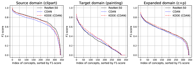
(a) clipart$\rightarrow$painting

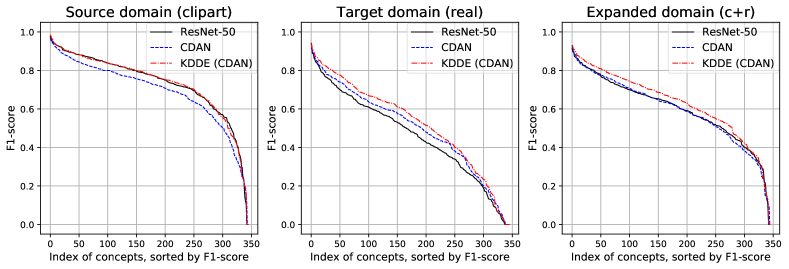
(b) clipart$\rightarrow$real

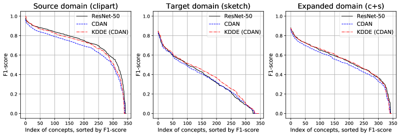
(c) clipart$\rightarrow$sketch

Figure 6. A concept-based comparison of ResNet-50, CDAN and KDDE (CDAN) on DomainNet. For the majority of the 345 concepts, KDDE(CDAN) is either better or comparable to the other two models on the target domain and on the expanded domain.

Fig. 6 shows a concept-based comparison of ResNet-50, CDAN and KDDE(CDAN) on three UDE tasks, i.e., clipart(c) $\rightarrow$ painting(p), clipart(c) $\rightarrow$ real(r) and clipart(c) $\rightarrow$ sketch(s). For the ease of comparison, for each model we have sorted all the 345 concepts in descending order according to their F1-scores. This allows us to measure the performance gap between the $j$-th best-performed concept of the models. As shown in the first column of Fig. 6, when tested on the source domain, the $150$-th best F1-score of ResNet-50 and KDDE (CDAN) is approximately $0.8$, while the corresponding position of CDAN is noticeably lower. The curve of KDDE(CDAN) is between ResNet-50 and CDAN, indicating that the performance of CDAN for the source domain has been recovered to some extent by KDDE. As for the target domain, see the middle column of Fig. 6, KDDE(CDAN)is higher than CDAN, followed by ResNet-50, proving that KDDE(CDAN) is also beneficial for the UDA task. As shown in the last column, KDDE(CDAN) scores the best for the majority of the concepts on the expanded domain.

4.4.4. Qualitative analysis

Fig. 1 presents the t-SNE (Maaten and Hinton, 2008) embedding of deep features learned by ResNet-50, CDAN and KDDE (CDAN) in the setting of clipart(c)$\rightarrow$painting(p). For better visualization, we only show test examples of 10 concepts selected at random from the top 30 best-performed concepts of ResNet-50. Across the source, target and expanded domains, intra-class data points tend to stay closer while inter-class data points are more distant in the feature space of KDDE(CDAN).

In order to better understand the behavior of the three models, we further employ Grad-CAM (Selvaraju et al., 2017) to visualize how the decisions are made. Fig. 5 shows Grad-CAM based heatmaps, where the first three rows and the last three rows are test images selected from the source (clipart) and the target (real) domains, respectively. Note that ResNet-50 clearly differs from CDAN in terms of their salient areas. By contrast, KDDE(CDAN) imitates ResNet-50 on the source domain (first three rows), yet resembles CDAN on the target domain (last three rows). These heatmaps demonstrate how KDDE adaptively learns from the two domain-specific models.

4.5. Experiments on OCT-11k

Results on OCT-11k measured in terms of confusion matrices, accuracy and AUC are summarized in Table 8. Similar to our previous experiments on Office-Home and DomainNet, the source-only ResNet-50 performs well on the source domain (Zeiss) but fails to generalize to the target domain (Topcon). Its confusion matrix shows that a large number of 334 true negatives are incorrectly classified as positive. This is in line with its ROC curve in Fig. 2c that the operating point with default cutoff of 0.5 produces a relatively larger False Positive Rate (FPR). Interestingly, while the ROC curve of CDAN is quite close to that of ResNet-50, its operating point given the same cutoff obtains a smaller FPR. The results suggest that UDA effectively improves the model’s insensitivity w.r.t. the value of the cutoff on the target domain. However, this advantage is obtained at the cost of noticeable performance drop on the source domain (0.8233 versus 0.8533 in accuracy and 0.8926 versus 0.9326 in AUC). By contrast, KDDE(CDAN) obtains the best overall performance, with no need of tuning the cutoff, justifying KDDE as a more principled approach to improving medical image classification in a multi-device scenario.

Table 8. Performance of three ResNet-50 models on OCT-11k, where ResNet-50 indicates the source-only model, followed by its counterparts trained by CDAN and KDDE(CDAN), respectively. Confusion matrices are shown in colored cells. KDDE(CDAN) is the best in terms of the overall performance.

			Source domain (Zeiss)				Target domain (Topcon)				Expanded domain (Zeiss+Topcon)
			$y$				$y$				$y$
Model			positive	negative	Accuracy	AUC	positive	negative	Accuracy	AUC	positive	negative	Accuracy	AUC
		positive	491	42			462	334			953	376
ResNet-50	$\hat{y}$	negative	90	277	0.8533	0.9326	9	95	0.6189	0.8593	99	372	0.7361	0.8534
		positive	471	49			453	204			924	253
CDAN	$\hat{y}$	negative	110	270	0.8233	0.8926	18	225	0.7533	0.8526	128	495	0.7883	0.8439
		positive	492	45			437	148			929	193
KDDE(CDAN)	$\hat{y}$	negative	89	274	0.8511	0.9200	34	281	0.7978	0.8985	123	555	0.8244	0.8914

4.6. Ablation Study

4.6.1. Alternative knowledge distillation loss?

We compare the KL divergence loss with two alternatives, i.e., the $l_{2}$ loss and the cross-entropy loss. As shown in Table 9, the KL divergence loss performs the best.

Table 9. Performance of KDDE (CDAN) with different losses on Office-Home.

Loss	Source domain	Target domain	Expanded domain
$l_{2}$	79.60	61.77	70.69
cross-entropy	80.78	63.19	71.99
KL divergence	81.44	63.90	72.67

4.6.2. The effect of knowledge distillation at the intermediate features space

Features that are discriminative of both domains shall allow an instance to be surrounded by instances of the same class. In order to verify if features obtained by KDDE are more discriminative, we consider cross-domain image retrieval, where each test image from one domain is used as a query example to retrieve images from the other domain. In particular, we conduct cross-domain image retrieval on two UDE tasks, i.e., C$\rightarrow$A and P$\rightarrow$R, on Office-Home. We compare ResNet-50, DDC and KDDE(DDC). Per model, the dissimilarity between two images $x$ and $x^{\prime}$ is defined as the $l_{2}$ distance between their 2,048-d features $F(x)$ and $F(x^{\prime})$. As Table 10 shows, using features of KDDE obtains higher precisions, indicating that cross-domain instances of the same class stay more closer in the intermediate feature space. Some qualitative results are presented in Fig. 7, where the top-5 returned items w.r.t. KDDE consistently exhibit domain-invariant visual patterns of sneakers. Both quantitative and qualitative results allow us to conclude that knowledge distillation results in more discriminative and domain-invariant feature representations.

Table 10. Performance of cross-domain image retrieval, using the 2,048-d features produced by the feature extractor $F$ of ResNet-50, DDC and KDDE (DDC), respectively. “Query S on T” means using each image in a source domain as a query example and performing retrieval in the target domain, while “Query T on S” indicates retrieval in the opposite direction. Performance metric: Precision at $N$ (P@N), $N=5,10$.

Model	C $\rightarrow$ A				P $\rightarrow$ R
	Query S on T		Query T on S		Query S on T		Query T on S
	P@5	P@10	P@5	P@10	P@5	P@10	P@5	P@10
ResNet-50	47.87	41.09	40.24	38.07	77.67	74.13	65.19	63.26
DDC	43.43	36.20	43.86	40.75	72.83	68.23	64.95	61.86
KDDE(DDC)	49.86	42.98	47.29	45.08	78.23	74.61	68.10	66.38

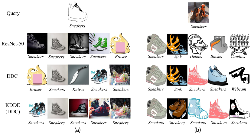
Figure 7. Visualization of cross-domain image retrieval. Each row corresponds to the top-5 retrieved images for queries from (a) the Clipart domain and (b) the Art domain, respectively. Note that image retrieval is fully content-based. Labels below each image are for illustration only.

4.6.3. KDDE for multi-domain shifts

Existing works on domain adaptation typically consider single-domain shift, where one wants to adapt a model for a single target domain, e.g., A$\rightarrow C$. We investigate a more challenging scenario of multi-domain shifts, which is to generalize the model simultaneously to multiple target domains, e.g., A$\rightarrow$ {C, P, R}. To that end, we improve CDAN by modifying its binary domain discriminator to support 4-way classification. We term the variant CDAN+. The performance of CDAN+ and KDDE (CDAN+) is reported in Table 11. Patterns similar to the previous single-domain shift experiments are observed. That is, CDAN+ outperforms the source-only ResNet-50 on the target domains but is less effective on the original source domain, while KDDE is better than CDAN+ on both source and multiple target domains. Consequently, KDDE obtains the overall best performance on the expanded domain.

Table 11. Performance of multi-domain shifts on Office-Home. A$\rightarrow${C,P,R} means using A as a source domain, which will be expanded to cover C, P and R. CDAN+ is our improved version of CDAN (Long et al., 2018) that performs 4-way classification in its domain discriminator. The source-only ResNet-50 is used as a reference. Performance increases (decreases) over this reference are shown in red (green).

Model	A$\rightarrow${C,P,R}
	A	C	P	R	A+C+P+R
ResNet-50	75.20	45.23	58.45	69.35	62.06
CDAN+	70.64$\downarrow$-4.56	50.23$\uparrow$+5.00	61.35$\uparrow$+2.90	67.17$\downarrow$-2.18	62.35$\uparrow$+0.29
KDDE(CDAN+)	72.59$\downarrow$-2.61	50.14$\uparrow$+4.91	63.49$\uparrow$+5.04	69.49$\uparrow$+0.14	63.93$\uparrow$+1.87
Model	C$\rightarrow${A,P,R}
	C	A	P	R	C+A+P+R
ResNet-50	78.91	47.06	57.55	59.65	60.79
CDAN+	77.09$\downarrow$-1.82	54.89$\uparrow$+7.83	66.53$\uparrow$+8.98	64.62$\uparrow$+4.97	65.78$\uparrow$+4.99
KDDE(CDAN+)	79.05$\uparrow$+0.14	57.67$\uparrow$+10.61	68.19$\uparrow$+10.64	66.94$\uparrow$+7.29	67.96$\uparrow$+7.17
Model	P$\rightarrow${A,C,R}
	P	A	C	R	P+A+C+R
ResNet-50	92.05	50.33	43.86	70.31	64.14
CDAN+	90.08$\downarrow$-1.97	54.24$\uparrow$+3.91	47.91$\uparrow$+4.05	70.90$\uparrow$+0.59	65.78$\uparrow$+1.64
KDDE(CDAN+)	91.33$\downarrow$-0.72	56.28$\uparrow$+5.95	50.50$\uparrow$+6.64	72.04$\uparrow$+1.73	67.54$\uparrow$+3.40
Model	R$\rightarrow${A,C,P}
	R	A	C	P	R+A+C+P
ResNet-50	84.11	63.62	48.23	76.27	68.06
CDAN+	82.01$\downarrow$-2.10	62.40$\downarrow$-1.22	57.14$\uparrow$+8.91	76.32$\uparrow$+0.05	69.47$\uparrow$+1.41
KDDE(CDAN+)	82.65$\downarrow$-1.46	63.30$\downarrow$-0.32	57.27$\uparrow$+9.04	77.97$\uparrow$+1.70	70.30$\uparrow$+2.24

4.6.4. Tackling UDE by tuning the trade-off parameter $\lambda$?

We report in Table 12 performance of DDC with the trade-off parameter $\lambda$ chosen from {0, 0.01, 0.1, 1, 10, 20, 100}, where $\lambda=10$ is the choice we have used so far. The peak performance is reached given $\lambda=0.01$, yet remains lower than KDDE. Moreover, by highlighting the best-performed $\lambda$ per domain using light-blue cells, we see that its optimal value is domain-dependent. Compared to simply tunning the trade-off parameter, KDDE is a more principled approach.

It is worth mentioning that DDC ($\lambda$=0) is not equivalent to the source-only ResNet-50. Because mini-batches sampled from the target domain have been used together with source mini-batches to estimate mean and variance of the Batch Normalization (BN) layers. This improves domain-variance of the intermediate features to some extent, and consequently leads to better performance (71.59 versus 70.11 in Table 12).

Table 12. Performance of DDC w.r.t. the trade-off parameter $\lambda$, on three tasks (C$\rightarrow$A, P$\rightarrow$R and R$\rightarrow$C) of Office-Home. Varied positions of light-blue cells, which indicate the best-performed $\lambda$ on specific domains, show the difficulty in selecting a proper $\lambda$ for tackling the UDE tasks.

Model		C$\rightarrow$A			P$\rightarrow$R			R$\rightarrow$C			Averaged accuracy on expanded domains
		C	A	C+A	P	R	P+R	R	C	R+C
ResNet-50		78.91	47.06	62.99	92.05	70.31	81.18	84.11	48.23	66.17	70.11
KDDE(DDC, $\lambda$=10)		80.05	54.57	67.31	92.67	73.36	83.02	83.24	53.86	68.55	72.96
DDC	$\lambda$=0	78.68	51.55	65.12	92.05	71.54	81.80	83.01	52.73	67.87	71.59
	$\lambda$=0.01	79.41	52.28	65.85	92.40	72.54	82.47	83.56	53.82	68.69	72.34
	$\lambda$=0.1	79.86	52.37	66.12	92.58	72.13	82.36	82.97	53.77	68.37	72.28
	$\lambda$=1	79.23	51.47	65.35	92.72	73.04	82.88	83.42	52.82	68.12	72.12
	$\lambda$=10	80.23	50.90	65.57	92.49	71.95	82.22	82.97	52.23	67.60	71.80
	$\lambda$=20	79.23	51.47	65.35	92.09	71.27	81.68	83.20	52.14	67.67	71.57
	$\lambda$=100	7.96	2.53	5.25	13.50	5.64	9.57	6.33	3.41	4.87	6.59

4.6.5. KDDE with MCD

As we have noted in Section 3, the UDA module of the proposed KDDE method can be implemented using any state-of-the-art UDA model. Here we instantiate the module using MCD (Saito et al., 2018). Again, ResNet-50 is used as their backbones. As shown in Table 13, KDDE(MCD) consistently outperforms MCD.

Table 13. Performance of MCD and KDDE (MCD). Per model we run the experiment three times, reporting the average value and standard deviation of the resultant accuracy scores.

Model	C$\rightarrow$A			P$\rightarrow$R
	C	A	C+A	P	R	P+R
MCD	77.53$\pm$0.66	51.90$\pm$0.96	64.72$\pm$0.53	91.45$\pm$0.32	70.67$\pm$0.71	81.06$\pm$0.51
KDDE(MCD)	79.20$\pm$0.35	56.33$\pm$0.65	67.77$\pm$0.49	92.25$\pm$0.16	73.91$\pm$0.10	83.08$\pm$0.04

4.6.6. Reproducibility test

Due to the large-scale datasets used in our study, producing Table 2 alone needs around 750 GPU hours, when running the related experiments in parallel on four GPU cards (two GTX 2080Ti plus two 1080Ti GPUs). Probably because of this reason, we rarely see reproducibility test in the literature of domain adaptation. Nonetheless, to reduce randomness, we run the experiments three times for all the tasks of Office-Home. As Table 14 shows, our major conclusion, i.e., the proposed KDDE is more effective, is again confirmed.

Table 14. Averaged performance of the individual models on Office-Home. Per model we repeat the training and evaluation procedures three times, reporting the averaged accuracy and standard deviation.

Model	A$\rightarrow$C			A$\rightarrow$P			A$\rightarrow$R
	A	C	A+C	A	P	A+P	A	R	A+R
ResNet-50	74.64$\pm$0.50	44.73$\pm$0.45	59.68$\pm$0.48	74.64$\pm$0.50	59.19$\pm$0.70	66.91$\pm$0.11	74.64$\pm$0.50	69.17$\pm$0.24	71.91$\pm$0.33
DDC	73.03$\pm$0.58	48.58$\pm$0.48	60.80$\pm$0.27	73.60$\pm$0.17	62.99$\pm$0.33	68.29$\pm$0.17	74.31$\pm$0.35	70.52$\pm$0.31	72.42$\pm$0.04
DANN	71.94$\pm$0.75	49.58$\pm$0.34	60.76$\pm$0.54	72.92$\pm$0.41	62.15$\pm$1.02	67.54$\pm$0.33	74.71$\pm$0.45	70.60$\pm$0.38	72.66$\pm$0.41
DAAN	73.68$\pm$0.33	49.00$\pm$0.08	61.34$\pm$0.18	74.28$\pm$0.29	63.93$\pm$0.33	69.10$\pm$0.04	74.74$\pm$0.48	71.25$\pm$0.30	73.00$\pm$0.38
CDAN	70.06$\pm$1.10	47.15$\pm$1.37	58.61$\pm$1.07	70.80$\pm$0.91	64.64$\pm$2.10	67.72$\pm$1.28	72.57$\pm$0.69	69.63$\pm$0.87	71.10$\pm$0.59
KDDE(DDC)	73.38$\pm$0.26	49.50$\pm$0.62	61.44$\pm$0.42	74.33$\pm$0.66	64.57$\pm$0.79	69.45$\pm$0.45	75.58$\pm$0.58	71.84$\pm$0.56	73.71$\pm$0.57
KDDE(CDAN)	68.84$\pm$1.08	47.98$\pm$0.84	58.41$\pm$0.94	71.53$\pm$0.80	66.20$\pm$1.93	68.87$\pm$1.32	73.68$\pm$0.29	71.19$\pm$1.14	72.43$\pm$0.71
Model	C$\rightarrow$A			C$\rightarrow$P			C$\rightarrow$R
	C	A	C+A	C	P	C+P	C	R	C+R
ResNet-50	78.98$\pm$0.09	48.20$\pm$1.28	63.59$\pm$0.65	78.98$\pm$0.09	58.31$\pm$0.69	68.65$\pm$0.37	78.98$\pm$0.09	59.85$\pm$0.35	69.42$\pm$0.17
DDC	79.74$\pm$0.44	51.93$\pm$0.91	65.84$\pm$0.24	80.03$\pm$0.38	61.75$\pm$0.74	70.89$\pm$0.18	79.53$\pm$0.66	64.01$\pm$0.51	71.77$\pm$0.56
DANN	78.06$\pm$0.23	53.10$\pm$0.91	65.58$\pm$0.52	78.86$\pm$0.69	60.41$\pm$1.24	69.64$\pm$0.82	78.89$\pm$0.03	62.93$\pm$0.33	70.91$\pm$0.15
DAAN	79.08$\pm$0.48	52.80$\pm$0.74	65.94$\pm$0.43	79.51$\pm$0.45	62.21$\pm$0.34	70.87$\pm$0.19	79.74$\pm$0.07	64.51$\pm$0.41	72.13$\pm$0.19
CDAN	78.09$\pm$0.30	53.59$\pm$1.28	65.84$\pm$0.59	78.27$\pm$0.64	65.34$\pm$0.69	71.81$\pm$0.33	79.12$\pm$0.14	64.66$\pm$0.64	71.89$\pm$0.33
KDDE(DDC)	80.09$\pm$0.48	55.57$\pm$0.89	67.83$\pm$0.47	80.43$\pm$0.33	64.06$\pm$0.79	72.25$\pm$0.53	80.47$\pm$0.42	66.64$\pm$1.34	73.55$\pm$0.85
KDDE(CDAN)	78.92$\pm$0.77	56.09$\pm$1.72	67.51$\pm$0.85	80.03$\pm$0.23	67.55$\pm$1.00	73.79$\pm$0.39	80.48$\pm$0.29	66.12$\pm$0.66	73.30$\pm$0.41
Model	P$\rightarrow$A			P$\rightarrow$C			P$\rightarrow$R
	P	A	P+A	P	C	P+C	P	R	P+R
ResNet-50	92.05$\pm$0.23	52.20$\pm$1.63	72.13$\pm$0.81	92.05$\pm$0.23	42.94$\pm$0.89	67.49$\pm$0.50	92.05$\pm$0.23	70.11$\pm$0.34	81.08$\pm$0.09
DDC	92.20$\pm$0.14	52.99$\pm$0.62	72.59$\pm$0.29	91.69$\pm$0.12	45.39$\pm$0.42	68.54$\pm$0.25	92.30$\pm$0.20	72.42$\pm$0.44	82.36$\pm$0.12
DANN	90.32$\pm$0.36	51.55$\pm$1.56	70.93$\pm$0.94	90.28$\pm$0.49	47.52$\pm$0.43	68.90$\pm$0.36	91.76$\pm$0.12	71.56$\pm$0.90	81.66$\pm$0.39
DAAN	92.06$\pm$0.50	54.21$\pm$0.87	73.14$\pm$0.37	91.63$\pm$0.24	45.24$\pm$1.05	68.44$\pm$0.61	92.38$\pm$0.21	72.37$\pm$0.22	82.38$\pm$0.18
CDAN	90.44$\pm$0.59	52.37$\pm$1.14	71.40$\pm$0.86	89.11$\pm$0.49	48.33$\pm$1.27	68.72$\pm$0.40	90.97$\pm$0.20	73.98$\pm$0.41	82.48$\pm$0.18
KDDE(DDC)	92.07$\pm$0.28	54.16$\pm$0.50	73.12$\pm$0.20	91.79$\pm$0.18	47.14$\pm$0.79	69.47$\pm$0.47	92.84$\pm$0.25	74.30$\pm$0.83	83.57$\pm$0.52
KDDE(CDAN)	90.81$\pm$0.67	53.40$\pm$1.96	72.10$\pm$1.31	89.96$\pm$0.45	49.73$\pm$0.83	69.84$\pm$0.33	92.14$\pm$0.31	75.23$\pm$0.42	83.68$\pm$0.33
Model	R$\rightarrow$A			R$\rightarrow$C			R$\rightarrow$P
	R	A	R+A	R	C	R+C	R	P	R+P
ResNet-50	84.05$\pm$0.07	63.73$\pm$0.49	73.89$\pm$0.22	84.05$\pm$0.07	49.47$\pm$1.08	66.76$\pm$0.51	84.05$\pm$0.07	76.14$\pm$0.74	80.09$\pm$0.36
DDC	84.49$\pm$0.26	64.52$\pm$0.50	74.50$\pm$0.30	83.21$\pm$0.28	53.23$\pm$0.87	68.22$\pm$0.54	84.02$\pm$0.33	77.79$\pm$0.42	80.91$\pm$0.24
DANN	83.76$\pm$0.41	65.33$\pm$0.33	74.55$\pm$0.13	82.00$\pm$0.69	55.07$\pm$0.96	68.54$\pm$0.78	82.83$\pm$0.43	78.02$\pm$0.08	80.43$\pm$0.23
DAAN	84.59$\pm$0.30	64.22$\pm$0.62	74.41$\pm$0.40	83.07$\pm$0.19	52.59$\pm$0.65	67.83$\pm$0.25	83.80$\pm$0.25	77.79$\pm$0.42	80.80$\pm$0.30
CDAN	82.29$\pm$0.90	64.19$\pm$0.51	73.24$\pm$0.70	80.12$\pm$0.38	54.82$\pm$1.38	67.47$\pm$0.68	82.45$\pm$0.22	80.12$\pm$0.37	81.29$\pm$0.25
KDDE(DDC)	84.65$\pm$0.30	65.22$\pm$0.66	74.94$\pm$0.47	83.33$\pm$0.08	54.03$\pm$0.33	68.68$\pm$0.19	83.91$\pm$0.16	79.27$\pm$0.88	81.59$\pm$0.52
KDDE(CDAN)	82.94$\pm$0.31	64.55$\pm$0.90	73.74$\pm$0.59	80.25$\pm$1.33	56.73$\pm$1.02	68.49$\pm$1.04	82.79$\pm$0.56	80.79$\pm$0.73	81.79$\pm$0.58

5. Conclusions

We have defined a new task termed unsupervised domain expansion (UDE). Accordingly, two benchmark datasets, i.e., Office-Home and DomainNet, have been re-purposed for the task. Our evaluation about four present-day domain adaptation models, either metric-based or adversarial, shows that their gain on the target domain is obtained at the cost of affecting their classification ability on the source domain. The proposed KDDE model effectively reduces such cost, and is found to be effective for both the new task and the traditional unsupervised domain adaptation task.

Acknowledgments. This research was supported in part by National Natural Science Foundation of China (No. 61672523), Beijing Natural Science Foundation (No. 4202033), the Fundamental Research Funds for the Central Universities and the Research Funds of Renmin University of China (No. 18XNLG19), and the Pharmaceutical Collaborative Innovation Research Project of Beijing Science and Technology Commission (No. Z191100007719002).

References

- (1)
- Asami et al. (2017) Taichi Asami, Ryo Masumura, Yoshikazu Yamaguchi, Hirokazu Masataki, and Yushi Aono. 2017. Domain adaptation of DNN acoustic models using knowledge distillation. In ICASSP.
- Ben-David et al. (2007) Shai Ben-David, John Blitzer, Koby Crammer, and Fernando Pereira. 2007. Analysis of representations for domain adaptation. In NeurIPS.
- Chen et al. (2017) Guobin Chen, Wongun Choi, Xiang Yu, Tony X Han, and Manmohan Chandraker. 2017. Learning efficient object detection models with knowledge distillation. In NeurIPS.
- De Fauw et al. (2018) Jeffrey De Fauw, Joseph R Ledsam, Bernardino Romera-Paredes, Stanislav Nikolov, Nenad Tomasev, Sam Blackwell, Harry Askham, Xavier Glorot, Brendan O’Donoghue, Daniel Visentin, et al. 2018. Clinically applicable deep learning for diagnosis and referral in retinal disease. Nature medicine 24, 9 (2018), 1342–1350.
- Duan et al. (2009) Lixin Duan, Ivor W. Tsang, Dong Xu, and Stephen J. Maybank. 2009. Domain Transfer SVM for video concept detection. In CVPR.
- French and Fisher (2018) Michal Mackiewicz French, Geoffrey and Mark Fisher. 2018. Self-ensembling for visual domain adaptation. In ICLR.
- Ganin et al. (2016) Yaroslav Ganin, Evgeniya Ustinova, Hana Ajakan, Pascal Germain, Hugo Larochelle, François Laviolette, Mario March, and Victor Lempitsky. 2016. Domain-Adversarial Training of Neural Networks. JMLR 17, 59 (2016), 1–35.
- Goldblum et al. (2020) Micah Goldblum, Liam Fowl, Soheil Feizi, and Tom Goldstein. 2020. Adversarially robust distillation. In AAAI.
- Hinton et al. (2015) Geoffrey Hinton, Oriol Vinyals, and Jeffrey Dean. 2015. Distilling the Knowledge in a Neural Network. In NIPS Deep Learning Workshop.
- Jiang et al. (2008) Wei Jiang, Eric Zavesky, Shih-Fu Chang, and Alex Loui. 2008. Cross-domain learning methods for high-level visual concept classification. In ICIP.
- Kang et al. (2019) Guoliang Kang, Lu Jiang, Yi Yang, and Alexander G. Hauptmann. 2019. Contrastive Adaptation Network for Unsupervised Domain Adaptation. In CVPR.
- Kermany et al. (2018) Daniel S Kermany, Michael Goldbaum, Wenjia Cai, Carolina CS Valentim, Huiying Liang, Sally L Baxter, Alex McKeown, Ge Yang, Xiaokang Wu, Fangbing Yan, et al. 2018. Identifying medical diagnoses and treatable diseases by image-based deep learning. Cell 172, 5 (2018), 1122–1131.
- Li et al. (2019) Shuang Li, Chi Harold Liu, Binhui Xie, Limin Su, Zhengming Ding, and Gao Huang. 2019. Joint Adversarial Domain Adaptation. In ACMMM.
- Liu et al. (2019) Yifan Liu, Ke Chen, Chris Liu, Zengchang Qin, Zhenbo Luo, and Jingdong Wang. 2019. Structured Knowledge Distillation for Semantic Segmentation. In CVPR.
- Long et al. (2015) Mingsheng Long, Yue Cao, Jianmin Wang, and Michael I. Jordan. 2015. Learning Transferable Features with Deep Adaptation Networks. In ICML.
- Long et al. (2018) Miingsheng Long, Zhangjie Cao, Jianmin Wang, and Micheal I Jordan. 2018. Conditional adversarial domain adaptation. In NeurIPS.
- Long et al. (2017) Mingsheng Long, Han Zhu, Jianmin Wang, and Michael I Jordan. 2017. Deep transfer learning with joint adaptation networks. In ICML.
- Maaten and Hinton (2008) Laurens van der Maaten and Geoffrey Hinton. 2008. Visualizing data using t-SNE. JMLR 9, Nov (2008), 2579–2605.
- Meng et al. (2019) Zhong Meng, Jinyu Li, Yashesh Gaur, and Yifan Gong. 2019. Domain adaptation via teacher-student learning for end-to-end speech recognition. In ASRU.
- Meng et al. (2018) Zhong Meng, Jinyu Li, Yifan Gong, and Biing-Hwang Juang. 2018. Adversarial teacher-student learning for unsupervised domain adaptation. In ICASSP.
- Mirzadeh et al. (2020) Seyed Iman Mirzadeh, Mehrdad Farajtabar, Ang Li, Nir Levine, Akihiro Matsukawa, and Hassan Ghasemzadeh. 2020. Improved knowledge distillation via teacher assistant. In AAAI.
- Paszke et al. (2019) Adam Paszke, Sam Gross, Francisco Massa, Adam Lerer, James Bradbury, Gregory Chanan, Trevor Killeen, Zeming Lin, Natalia Gimelshein, Luca Antiga, Alban Desmaison, Andreas Kopf, Edward Yang, Zachary DeVito, Martin Raison, Alykhan Tejani, Sasank Chilamkurthy, Benoit Steiner, Lu Fang, Junjie Bai, and Soumith Chintala. 2019. PyTorch: An imperative style, high-performance deep learning library. In NeurIPS.
- Peng et al. (2019) Xingchao Peng, Qinxun Bai, Xide Xia, Zijun Huang, Kate Saenko, and Bo Wang. 2019. Moment matching for multi-source domain adaptation. In ICCV.
- Pinheiro (2018) Pedro O Pinheiro. 2018. Unsupervised domain adaptation with similarity learning. In CVPR.
- Romero et al. (2015) Adriana Romero, Nicolas Ballas, Samira Ebrahimi Kahou, Antoine Chassang, Carlo Gatta, and Yoshua Bengio. 2015. FitNets: Hints for thin deep nets. ICLR (2015).
- Saito et al. (2019) Kuniaki Saito, Donghyun Kim, Stan Sclaroff, Trevor Darrell, and Kate Saenko. 2019. Semi-Supervised Domain Adaptation via Minimax Entropy. In ICCV.
- Saito et al. (2018) Kuniaki Saito, Kohei Watanabe, Yoshitaka Ushiku, and Tatsuya Harada. 2018. Maximum classifier discrepancy for unsupervised domain adaptation. In CVPR.
- Saputra et al. (2019) Muhamad Risqi U Saputra, Pedro P B De Gusmao, Yasin Almalioglu, Andrew Markham, and Niki Trigoni. 2019. Distilling Knowledge From a Deep Pose Regressor Network. In ICCV.
- Selvaraju et al. (2017) Ramprasaath R. Selvaraju, Michael Cogswell, Abhishek Das, Ramakrishna Vedantam, Devi Parikh, and Dhruv Batra. 2017. Grad-CAM: Visual Explanations From Deep Networks via Gradient-Based Localization. In ICCV.
- Shi et al. (2019) Yangyang Shi, Mei-Yuh Hwang, Xin Lei, and Haoyu Sheng. 2019. Knowledge distillation for recurrent neural network language modeling with trust regularization. In ICASSP.
- Sun and Saenko (2016) Baochen Sun and Kate Saenko. 2016. Deep CORAL: Correlation Alignment for Deep Domain Adaptation. In ECCV Workshop.
- Tian et al. (2020) Yonglong Tian, Dilip Krishnan, and Phillip Isola. 2020. Contrastive representation distillation. ICLR.
- Toldo et al. (2020) Marco Toldo, Andrea Maracani, Umberto Michieli, and Pietro Zanuttigh. 2020. Unsupervised Domain Adaptation in Semantic Segmentation: A Review. Technologies 8, 2 (2020), 35.
- Tzeng et al. (2017) Eric Tzeng, Judy Hoffman, Kate Saenko, and Trevor Darrell. 2017. Adversarial discriminative domain adaptation. In CVPR.
- Tzeng et al. (2014) Eric Tzeng, Judy Hoffman, Ning Zhang, Kate Saenko, and Trevor Darrell. 2014. Deep Domain Confusion: Maximizing for Domain Invariance. ArXiv abs/1412.3474 (2014).
- Venkateswara et al. (2017) Hemanth Venkateswara, Jose Eusebio, Shayok Chakraborty, and Sethuraman Panchanathan. 2017. Deep Hashing Network for Unsupervised Domain Adaptation. In CVPR.
- Wang et al. (2019c) Weisen Wang, Zhiyan Xu, Weihong Yu, Jianchun Zhao, Jingyuan Yang, Feng He, Zhikun Yang, Di Chen, Dayong Ding, Youxin Chen, and Xirong Li. 2019c. Two-Stream CNN with Loose Pair Training for Multi-modal AMD Categorization. In MICCAI.
- Wang et al. (2019a) Ximei Wang, Ying Jin, Mingsheng Long, Jianmin Wang, and Michael I Jordan. 2019a. Transferable Normalization: Towards Improving Transferability of Deep Neural Networks. In NeurIPS.
- Wang et al. (2019b) Ximei Wang, Liang Li, Weirui Ye, Mingsheng Long, and Jianmin Wang. 2019b. Transferable attention for domain adaptation. In AAAI.
- Yang et al. (2007) Jun Yang, Rong Yan, and Alexander G. Hauptmann. 2007. Cross-domain video concept detection using adaptive SVMs. In ACMMM.
- Yang Zou (2019) Xiaofeng Liu B. V. K. Vijaya Kumar Jinsong Wang Yang Zou, Zhiding Yu. 2019. Confidence regularized self-training. In ICCV.
- Yu et al. (2019) Chaohui Yu, Jindong Wang, Yiqiang Chen, and Meiyu Huang. 2019. Transfer Learning with Dynamic Adversarial Adaptation Network. In ICDM.
- Zhang et al. (2019a) Linfeng Zhang, Jiebo Song, Anni Gao, Jingwei Chen, Chenglong Bao, and Kaisheng Ma. 2019a. Be your own teacher: Improve the performance of convolutional neural networks via self distillation. In ICCV.
- Zhang et al. (2019b) Peng Zhang, Li Su, Liang Li, BingKun Bao, Pamela Cosman, GuoRong Li, and Qingming Huang. 2019b. Training Efficient Saliency Prediction Models with Knowledge Distillation. In ACMMM.
- Zhang et al. (2018a) Quanshi Zhang, Wenguan Wang, and Song-Chun Zhu. 2018a. Examining CNN Representations with Respect to Dataset Bias. In AAAI.
- Zhang et al. (2018b) Ying Zhang, Tao Xiang, Timothy M Hospedales, and Huchuan Lu. 2018b. Deep mutual learning. In CVPR.
- Zou et al. (2018) Yang Zou, Zhiding Yu, BVK Vijaya Kumar, and Jinsong Wang. 2018. Unsupervised domain adaptation for semantic segmentation via class-balanced self-training. In ECCV.