High Power Backward Wave Oscillator using Folded Waveguide with Distributed Power Extraction Operating at an Exceptional Point

Abstract

The concept of exceptional point of degeneracy (EPD) is used to conceive a degenerate synchronization regime that is able to enhance the level of output power and power conversion efficiency for backward wave oscillators (BWOs) operating at millimeter-wave and Terahertz frequencies. Standard BWOs operating at such high frequency ranges typically generate output power not exceeding tens of watts with very poor power conversion efficiency in the order of 1%. The novel concept of degenerate synchronization for the BWO based on a folded waveguide is implemented by engineering distributed gain and power extraction along the slow-wave waveguide. The distributed power extraction along the folded waveguide is useful to satisfy the necessary conditions to have an EPD at the synchronization point. Particle-in-cell (PIC) simulation results shows that BWO operating at an EPD regime is capable of generating output power exceeding 3 kwatts with conversion efficiency of exceeding 20% at frequency of 88.5 GHz.

I Introduction

The capability to generate significant power at millimeter-wave and terahertz (THz) frequencies using vacuum electronics sources has motivated many investigations due to the their high demand on applications such as imaging, spectroscopy and communications [1, 2, 3, 4, 5, 6]. Vacuum electronic devices operating at millimeter-wave and THz frequencies often use folded waveguides (serpentine-shaped waveguide) as shown in Fig. 1. The advancement of fabrication technologies such as LIGA (LIthographie, Galvanoformung, Abformung) have made it easy to fabricate and develop vacuum electronic devices operating at these high frequencies [7, 8, 9, 10, 11, 4].

Exceptional points of degeneracy (EPD) are points in parameter space of a system at which two or more eigenmodes coalesce. Despite most of the published work on EPDs are related to parity time (PT) symmetry [12, 13], the occurrence of EPDs does not necessarily require a system to exactly satisfy the PT symmetry condition. In general, but not always [14, 15, 16] , the occurrence of EPD in waveguides requires simultaneous presence of gain and loss [17, 15]. Instead of using losses, the EPD in this work is enabled by the distributed power extraction (DPE) from the folded waveguide as shown in Fig. 1. The ideal concept of simultaneous radiation losses and distributed gain in two coupled waveguides leading to an EPD was already discussed in [17] in a theoretical setting. In this paper the concept is achieved using a single serpentine waveguide coupled to an electron beam (e-beam). The energy extracted from the e-beam and delivered to the guided electromagnetic (EM) mode is considered as a distributed gain from the waveguide perspective, whereas DPE represents extraction “losses” and not mere dissipation [18, 19, 20]. The distributed extracted power from the discrete waveguide ports along the serpentine (Fig. 1) could be directed toward an array antenna and hence radiated generating a collimated EM beam or could be collected in an external waveguide after proper optimization for power combining.

In [19], we have studied the theoretical and idealistic analysis of a BWO with degenerate synchronization operating at an EPD (we named it EPD-BWO) using a generalized Pierce model [21] that accounts for waveguide with distributed power extraction modeled as losses. Here we show analytically and numerically using particle-in-cell (PIC) simulations that an EPD-BWO is characterized by the asymptotic trend of the starting e-beam dc current that decreases quadratically with slow wave structure (SWS) length to a non-vanishing value that can be properly designed based on the required output power. In this paper, we focus on the realization and implementation of the degenerate synchronization of the EPD-BWO at millimeter-waves since it is very challenging to generate significant power levels at such high frequencies. Though we do not show it here, the concept of degenerate synchronization is expected to be advantageous also at THz frequencies. The use of EPD enables to have higher starting current for oscillation which indicates higher level of power extraction from the e-beam kinetic energy.

Works on BWOs operating at millimeter-wave and THz have reported a generated output power not exceeding tens of watts with power conversion efficiency around 1% [22, 23, 10, 24, 25, 26, 27, 6]. In this paper we employ the concept of EPD to enhance such poor efficiency and to increase the level of output power. We asses the advancements in the performance of BWO operating at an EPD (EPD-BWO) over a standard BWO (STD-BWO) using particle-in-cell (PIC) simulations.

II Implementation of degenerate synchronism regime based on EPD in a folded waveguide

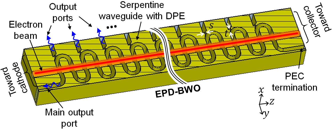
Figure 1: BWO with folded waveguide operating at millimeter waves: (a) standard (STD)-BWO where the power is extracted from a waveguide end; (b) EPD-BWO where the power is extracted in a distributed fashion to enable the occurrence of the degenerate synchronization regime when working at an EPD [18, 19, 20]. The distributed power is extracted by introducing a small slot in each folded waveguide period that couples portion of the power in the folded waveguide to the outgoing rectangular waveguides.

A simple model for the interaction between the e-beam and the EM wave in vacuum tube devices was provided by Pierce in [21]. Augmenting the Pierce model to include SWSs with distributed loads, we have shown in [18, 19, 20] that a second order EPD is found as a special degeneracy of the interactive (hybrid) modes when DPE along the waveguide is added and when the beam dc current is set to specific value $I_{0}=I_{0e}$, i.e., using this e-beam dc current guarantees that two modes in the interactive system are synchronized. The e-beam dc current $I_{0e}$ is the specific value that guarantees the degeneracy of two modes, which can be set to a desired value by properly designing the interactive SWS system. The cold SWS with DPE has a complex propagation constant $\beta_{c}=\beta_{cr}+i\beta_{ci}$ around the synchronization point, where the imaginary part $\beta_{ci}$ accounts for the DPE along the SWS and the subscript $c$ denotes circuit that is representing the cold SWS. We have shown in [18, 19, 20] that the EPD e-beam dc current has a proportionality $I_{0e}\propto\beta_{ci}^{2}$, where the parameter $\beta_{ci}$ represents the DPE introduced in the SWS and is determined by engineering the DPE from the SWS. The fact that an EPD e-beam current $I_{0e}$ is found for any amount of desired distributed power extraction implies that this so called “degenerate synchronization” regime is guaranteed for any desired high power generation. Therefore, in principle, the synchronism is maintained for any desired distributed power output, according to the augmented Pierce-based model presented in [18, 19]. Note that this trend is definitely not observed in standard BWOs where interactive modes are non-degenerate and the load is at one end of the SWS. Furthermore in a STD-BWO the starting (i.e., threshold) current vanishes with increasing SWS length, whereas in an EPD-BWO it decreases quadratically to a fixed, desired, value [18, 19, 20], that coincides with $I_{0e}\propto\beta_{ci}^{2}$, hence this value is related to the amount of DPE. Therefore, the degenerate regime enables a large transfer of power from the e-beam to the waveguide EM mode as compared to a standard regime.

Here, we show how to implement the EPD regime in a BWO that uses a folded waveguide and operating at millimeter wave and THz frequency through introducing DPE along the waveguide as illustrated in Fig. 1. In particular, we consider a folded waveguide made of copper with rectangular cross-section of dimension $a=1.9$ mm and $b=0.2$ mm. The folded waveguide has a bending radius of $R_{s}=0.3$ mm and the straight sections have length of $h=1$ mm. The beam tunnel radius is $R_{t}=0.175$ mm, with a filling factor of about 58%, i.e., the e-beam has radius of $R_{b}=0.13$ mm. The DPE is conceived in the waveguide by making a small rectangular slot of dimensions $a\times s$, with $s=0.05$ mm, in the wide side of the rectangular cross section, and length $t=0.1$ mm, in each period of the waveguide (as shown in Fig. 1). The slots couples portion of the main power in the SWS to an outgoing rectangular waveguide with dimensions $a\times b$, as shown in Fig. 2(b).

Figure 2(c) shows a comparison between the dispersion relation of EM modes in two “cold” SWSs: one used in a STD-BWO in Fig. 2(a), and one used in the BWO with DPE in Fig. 2(b). The dispersion curves show only the dominant EM mode $\mathrm{TE_{10}}$ which exhibits an axial (longitudinal, along the folded waveguide) electric field component able to interact with the e-beam. The dispersion curves in Fig 2(c) show that the cold SWS with DPE supports backward waves that have a propagation constant with non-zero imaginary part $\beta_{ci}$ at the frequencies where the interaction with the e-beam may occur. The imaginary part of a mode propagating in the folded waveguide without DPE is almost equal to zero at the interaction points ($\omega/\beta_{cr}\approx u_{0}$, where $u_{0}$ is the electrons average speed and $\omega$ is the angular frequency). The complex wavenumber dispersion relation in presence of DPE, shown in Fig 2(c), is obtained by simulating a single unit-cell that is connected to two ports at its beginning and end, while the power extraction waveguide is connected to a matched port, and the beam tunnel ends are terminated by prefect electric conductor (PEC) since the $\mathrm{TE_{10}}$ mode is below cutoff of such a tunnel (we have checked that varying the beam tunnel length and terminations does not affect the result). The Finite Element Frequency Domain solver implemented in CST Studio Suite by DS SIMULIA is used to calculate the two-port scattering parameters which are converted into a two-port transfer matrix representing one unit-cell. The complex Floquet-Bloch modes wavenumbers are then obtained by enforcing periodic boundaries for the obtained transfer matrix, following the method discussed in [28].

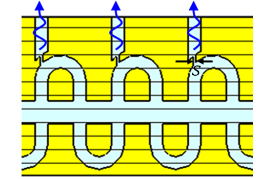
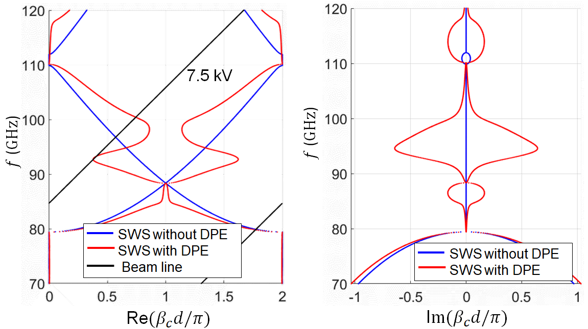
Figure 2: Longitudinal cross-sections of a folded waveguide without (a) and with DPE (b). (c) Dispersion of EM guided modes in the “cold” waveguide in (a) and (b), without (blue curve) and with (red curve) DPE, respectively. The dispersion shows the real and imaginary parts of the complex wavenumber. The non-zero imaginary part of the wavenumbers of the EM mode with DPE (red line) shows that the waveguide in (b) exhibits distributed power extraction. The imaginary part of the mode without DPE (blue line) is almost zero.

III Particle-in-cell simulations of degenerate synchronous regime in BWO

We perform PIC simulations to assess the performance and features of the proposed EPD-BWO using a folded waveguide and operating at millimeter wave frequency. The PIC simulations uses a pencil e-beam with dc voltage $V_{0}=7.5$ kV and an axial dc magnetic field of 2 T to confine the e-beam.

III-A Starting current

We start first by studying the starting (threshold) current of oscillation to see how much increase in starting current we obtain with the EPD-BWO with respect to a STD-BWO without DPE. Results show that the EPD-BWO exhibits a much higher starting current of oscillation with respect to a STD-BWO without DPE. Indeed the increase in starting current is an advantage here because it enables to push up the saturation power level of the BWO to much higher levels and therefore leads to a high level of power extraction. The output power for a STD-BWO is extracted from the main port at the left end of the waveguide, whereas the output power of the EPD-BWO is extracted from the left waveguide port in addition to all DPE waveguide ports as shown in Fig. 1. Fig. 3 shows the output ports signals, obtained from PIC simulations, for both BWOs with 13 unit cells when the e-beam current is just below and above the starting currents of each BWO (the threshold currents have been found by repeating simulations with varying e-beam dc current values with steps of 0.1 A for the STD-BWO and 0.01 A for the EPD-BWO). A self-standing oscillation frequency of 93.1 GHz is observed when the beam dc current $I_{0}$ is at or larger than $0.8$ A for the STD-BWO case, whereas a self-standing oscillation frequency of 88.2 GHz is observed when the beam dc current $I_{0}$ is at or larger than $2.16$ A for the EPD-BWO case. We estimate the starting current of the oscillation as the average of the two observed values of the e-beam currents where oscillation starts to occur and does not occur, respectively. Therefore,the starting currents $I_{st}$ for STD-BWO and EPD-BWO are0.75 A and 2.15 A, respectively. Considering larger and larger numbers of unit cells implies that $I_{st}\to 0$ for the STD-BWO case, and $I_{st}\to I_{0e}$ for the EPD-BWO case [19, 20].

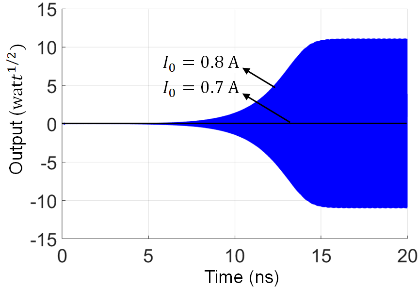
Figure 3: Output signals for: (a) STD-BWO and (b) EPD-BWO, both having 13 unit-cells, when the e-beam dc current is just below and above the starting current of oscillation ($I_{st}$) for each BWO case. The output signal for the STD-BWO is extracted at the left-end port of the waveguide (a), whereas for the EPD-BWO the signals are extracted from the 13 distributed ports and from the left-end port, denoted by different colored curves (b).

To assess the occurrence of an EPD, we verify the unique scaling trend of the starting current in (4) by repeating the previous study for different SWS lengths. Such scaling trends for the starting current for both STD-BWO and EPD-BWO are shown using black dots in Fig. 4 based on PIC simulation results, varying the number of periods of the SWS. The dashed lines represent fitting curves; the case of EPD-BWO shows very good agreement with the fitting curve. The EPD-BWO is characterized by a starting current that does not tend to zero as the SWS length increases, in contrast to the starting current of a STD-BWO that vanishes for increasing SWS length. The observed scaling of the starting current of a EPD-BWO is a quadratic function of the inverse of the SWS length, which is the same trend observed theoretically in [19] using an augmented Pierce model. Indeed, we have shown in [19, 20] that the starting current of oscillation for EPD-BWO scales with the SWS length as

$$I_{st}=I_{0e}+\left(\dfrac{\alpha}{N}\right)^{2},$$ (1)

where $\alpha$ is a constant. From the fitting shown in Fig. 4 we have found that $I_{st}=2.09+(3.2/N)^{2},$therefore, following [19], the estimate of the EPD current is $I_{0e}=I_{st}|_{N\to\infty}=2.09$ A. Later on in the next section, we show that the use of a current close to this value will lead to the degeneracy of two hybrid modes in the dispersion of the hot structure, using data extracted from PIC simulations.

Figure 4: Scaling of starting e-beam dc current for STD-BWO and EPD-BWO with SWSs length (black dots). Dashed lines represent fitting curves. The EPD-BWO shows a starting current trend that does not vanish for long lengths, the quadratic decay is representative of a degeneracy condition.

III-B Power performance: EPD-BWO compared to a STD-BWO

Figure 5: Comparison between the output power and power conversion efficiency of a STD-BWO and an EPD-BWO, both based on the same folded waveguide SWS, without and with DPE, respectively. In (a) we observe the power trends when varying the number of unit cells of the folded waveguide when the used beam dc current is 10% higher than the starting currents for the STD-BWO and EPD-BWO, and for each length. In (b) we observe the power trends when varying the the beam dc current, assuming the SWSs for the two BWOs are made of 20 unit cells. The figure shows that EPD-BWO has much higher efficiency at much higher level of power generation compared to the STD-BWO.

We calculate the output power for STD-BWO and EPD-BWO when the e-beam is 10% above the starting beam current for each case, i.e., $I_{0}=1.1I_{st}$, where the starting currents for both the EPD-BWO and STD-BWO are shown in Fig. 4. The output power $P_{out}$ for the EPD-BWO case is calculated as the sum of the power delivered to the distributed ports and the main port. We show in Fig. 5 the output power and power conversion efficiency, defined as $\eta=P_{out}/(V_{0}I_{0})$, for both cases of EPD-BWO and STD-BWO when varying the number of periods (i.e., unit cells) of the folded waveguide . The figure shows that the EPD-BWO has always much higher output power level and power conversion efficiency as compared to the STD-BWO. We observe from the figure also that the output power and efficiency for the EPD-BWO increase as we increase the number of folded waveguide periods, unlike for the STD-BWO.

We then show in Fig. 5 the output power and power conversion efficiency for both cases of EPD-BWO and STD-BWO when changing the beam dc current, keeping the number of period equal to $N=20$ for both kinds of BWOs. The figure shows that when the beam dc current is exceeding the starting current for each of the EPD-BWO and STD-BWO, the EPD-BWO is achieving much higher power conversion efficiency at much higher level of power extraction. Note that we sweep the current for a larger range for the STD-BWO case to be able reach the level of currents that is used for EPD-BWO to be able to have a fair comparison. Maximum output power is achieved for EPD-BWO case when the used current is $I_{0}=2.6$ A which is about 22% higher than the starting current of oscillation and 24% higher than the EPD current $I_{0e}$ estimated from Fig. 4. We expect that longer length of the folded waveguide we use, the closer we are to the EPD and higher efficiency and output power are obtained.

IV Degenerate dispersion relation for the hot structure based on PIC simulation

The goal of this section is to show the degeneracy of the wavenumbers of the modes of the interactive system (i.e, the hybrid modes) using PIC simulations. Previously the degenerate dispersion has been shown only using the approximate analytical method based on the Pierce model in [19]. Using the idealized analytical method we also demonstrated the degeneracy of two eigenvectors at the EPD [19]. Here we adopt the general numerical procedure described in [29] to estimate the wavenumbers of the interactive (hybrid) modes, and show the hybrid mode degeneracy using data extracted from PIC simulations. The advantage is that PIC simulations predict the behavior of a realistic structure, while the model in [19] was just based on Pierce theory. The procedure is based on exciting the structure from both sides of the SWS by EM waves having monochromatic signal as illustrated in Fig. 6, and then calculating the state vectors that describe the EM field and the e-beam dynamics at discrete periodic locations along the SWS. The time domain data extracted from PIC simulations are transformed into phasors after reaching a steady state regime as described in [29]. We then find the transfer matrix associated to a unit-cell of the “hot” SWS that best relates the calculated state vectors at both ends of each unit cell. Once the estimate of the unit-cell transfer matrix is obtained, we find the hybrid eigenmodes in a hot SWS using Floquet theory. We provide details about the steps we used to generate the dispersion relation for the hot SWS in Appendix A.

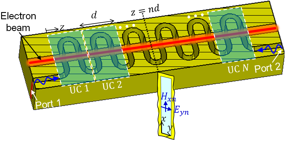
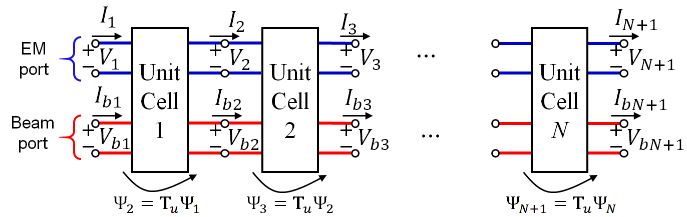
Figure 6: (a) Setup used to determine the complex-valued wavenumber versus frequency dispersion relation of the hybrid modes in the hot SWS based on data extracted from PIC simulations. (b) Circuit model showing that each unit cell in the hot SWS is modeled as four-port network circuit with equivalent voltages and currents representing EM waves ($V_{n}$, $I_{n}$) and space-charge waves ($V_{bn}$, $I_{bn}$) dynamics.

The wavenumber-frequency dispersion describing the complex-valued wavenumber of the hybrid eigenmodes in the hot SWS is determined by running multiple PIC simulations for a SWS made of 11 unit-cells, at different frequencies and at different beam dc currents, and then determining the transfer matrix of the unit-cell at each frequency and current combination using Eq. (8). We sweep the e-beam dc current around the expected value of EPD beam current $I_{0e}$, which is the value of e-beam current pertaining to the infinitely long SWS according to the fitting shown in Fig. 4; the use a current that is close to this current value should guarantee the coalescence of two interactive beam-EM modes. It is important to mention that the used beam currents to generate the results in this section are below the starting current of oscillation which is estimated to be 2.175 A as shown in Fig. 4, in order to avoid strong saturation regimes proper of oscillators’ dynamics. Therefore, by neglecting nonlinearities, one models each unit-cell of the hot SWS using a transfer matrix as discussed previously and in Appendix A. Since the transfer matrix has dimension 4x4, there are four eigenvalues, i.e., for complex-valued wavenumbers associated to the four hybrid modes supported by the model shown in Fig. 6. We plot only the three modes that have a wavenumber with a positive real part. The dispersion diagram of such three interactive modes in the hot EM-electron beam system is shown in Fig. 7 at different e-beam dc current. The figure shows a degeneracy of two hybrid modes (the red and blue curves) at a frequency near $f=88.8$ GHz which is very close to the oscillation frequency when the used e-beam dc current is around $I_{0}=2.055$A which is close to (and slightly lower) the value of EPD beam current value of $I_{0e}=I_{st}|_{N\to\infty}=2.09$ obtained from the fitting shown in Fig. 4, calculated as a limit for an infinitely long SWS. All the e-beam currents $I_{0}$ considered show that two wavenumbers are either close to the degeneracy or degenerate. There is only a very small discrepancy between the estimate of EPD current $I_{0e}$ obtained from the fitting of the starting currents varying length and from observing the degeneracy of two hybrid modes shown in Fig. 7. Such small discrepancy could be attributed to the use of finite precision in calculating the starting current of oscillation, or to the approximations implied in the retrieval method used to obtain the dispersion of hot structure, like possible nonlinearites that are not accounted for in our retrieval model.

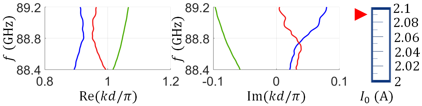
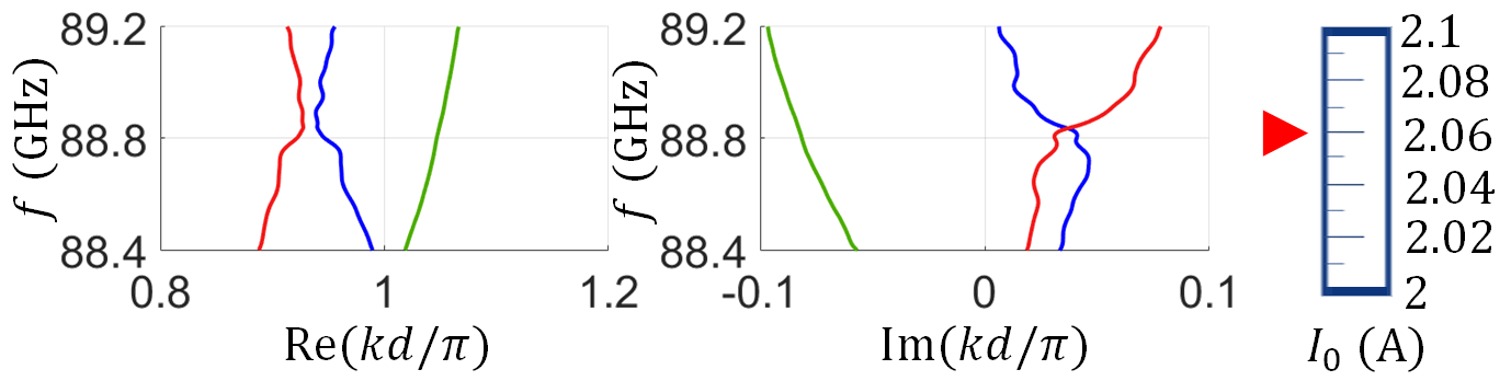
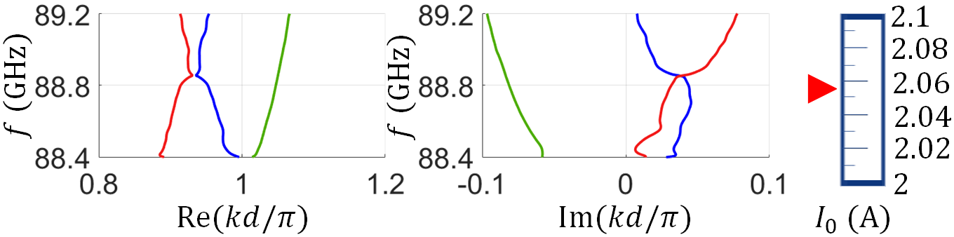
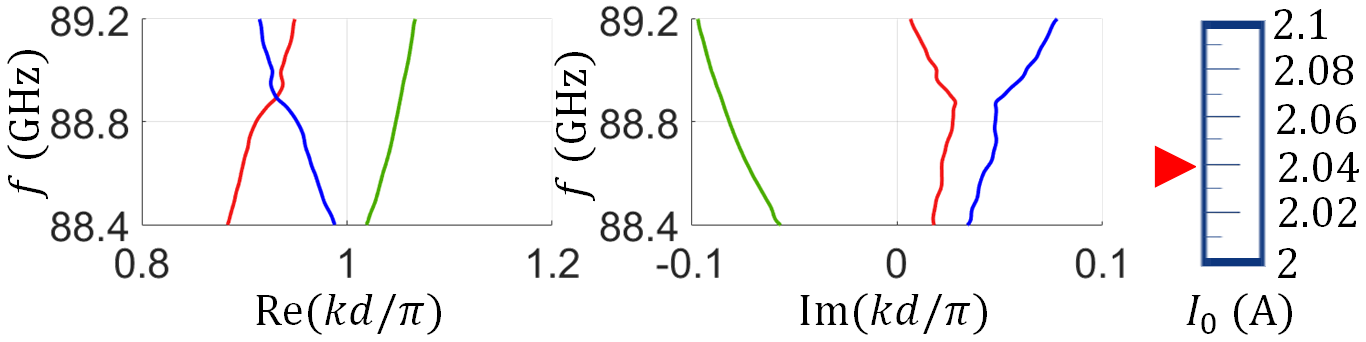
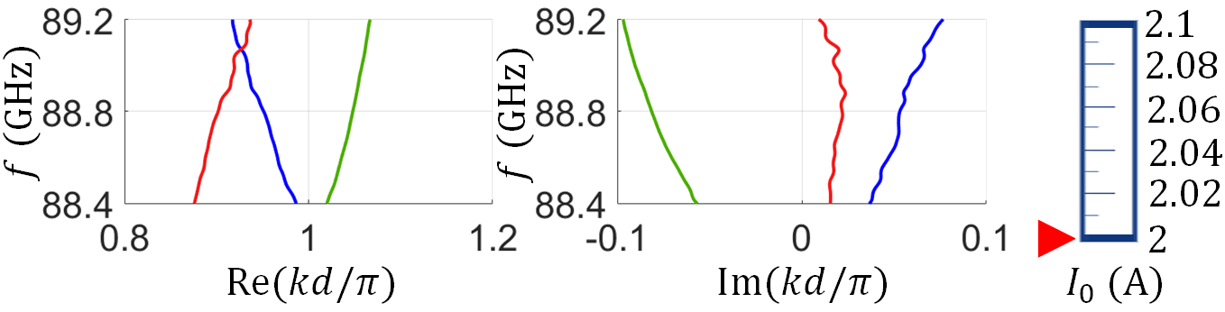
Figure 7: Dispersion of complex-valued wavenumbers of three hybrid modes showing the wavenumber degeneracy at about $I_{0}=2.055$A. Wavenumbers of the three modes with positive real part are retrieved from data obtained by PIC simulations relative to hot SWSs with 11 unit-cells, when using different e-beam dc current: (a)$I_{0}=2.09$A, (b)$I_{0}=2.06$A, (c)$I_{0}=2.055$A, (d)$I_{0}=2.04$ and (e)$I_{0}=2.00$A. All the considered beam dc currents to generate the results are lower than the starting current of oscillation which is estimated to be 2.175 A when using 11 unit cells. The plots show a modal degeneracy when the the beam dc current is about $I_{0}=2.055$A, which is very close to the EPD current value of $I_{0e}=2.09$ estimated using the fitting in Fig. 4, and the operating frequency at which the degeneracy is observed is about $f=88.8$ GHz, which is close to the oscillation frequency.

V Conclusion

We have conceived a degenerate synchronization regime to increase the output power and power conversion efficiency of BWOs operating at millimeter wave and THz frequencies. The degenerate synchronization regime is achieved through altering the folded waveguide by adding periodic power extraction ports. This allows the interactive system to work at an EPD which implies a maintained synchronism designed for any desired level of power extraction. PIC simulation results shows that a millimeter wave BWO operating at degenerate synchronization regime is capable of generating output power exceeding 3 kwatts with conversion efficiency of exceeding 20% at a frequency of 88.5 GHz. The unique quadratic starting current scaling law with waveguide interaction lengths observed from PIC simulations demonstrates the EPD-based synchronization phenomenon, compared to that in a STD-BWO that has a starting current law that vanishes cubically. The complex-valued wavenumber degeneracy is confirmed by elaborating data extracted from PIC simulations which implies the existence of EPD in the interactive system. This new degenerate synchronization regime may pave the way to the realization of very high power sources at millimeter and submillimeter waves, with high power conversion efficiency.

VI Acknowledgment

This material is based upon work supported by the Air Force Office of Scientific Research award number FA9550-18-1-0355. The authors are thankful to DS SIMULIA for providing CST Studio Suite that was instrumental in this study.

Appendix A Method used to find the dispersion of hybrid hot modes using data from PIC simulations

We provide the basic steps of the retrieval method used to generate the dispersion relations for hot SWSs based on time domain data obtained from PIC simulations. The reader is addressed to [29] for more details.

We define a state vector that describes the EM and space-charge waves, defined at discrete periodic locations $z=z_{n}=nd$ as

$$\mathbf{\Psi}_{n}=[\begin{array}[]{cccc}V_{n},&I_{n},&V_{bn},&I_{bn}\end{array}]^{T},$$ (2)

where $V_{n}$ and $I_{n}$ are equivalent voltages and currents representing the EM mode in the SWS, and $V_{bn}$ and $I_{bn}$ are equivalent voltages and currents representing the charge wave modulating the e-beam.

We assume that the EM field in the folded rectangular waveguide is dominated by a $\mathrm{TE_{10}}$. Thus the (locally-) transverse field at the rectangular cross section is in the form of

$$\begin{array}[]{c}\mathbf{E}_{tn}(x,y)=E_{yn}\sin\left(\dfrac{\pi x}{a}\right)\mathbf{a}_{y},\\ \mathbf{H}_{tn}(x,y)=H_{xn}\sin\left(\dfrac{\pi x}{a}\right)\mathbf{a}_{x},\end{array}$$ (3)

The coordinates used here do not described the waveguide folding, we just use them to describe the field at cross sections of the rectangular waveguide at discrete locations $z=z_{n}$. We use an equivalent transmission line model that has voltage and current $V_{n}$ and $I_{n}$ representing the EM field in the periodic SWS. The voltage and current are calculated as the projection of the transverse electric and magnetic fields in the SWS on the electric and magnetic transverse eigenvector basis proper of a $\mathrm{TE_{10}}$ mode as explained in [30, 31, 32]

$$\begin{array}[]{c}V_{n}=\langle\mathbf{E}_{tn}(x,y),\mathbf{e}(x,y)\rangle,\\ I_{n}=\langle\mathbf{H}_{tn}(x,y),\mathbf{h}(x,y)\rangle,\end{array}$$ (4)

where $\langle\mathbf{A},\mathbf{B}\rangle=\int_{0}^{a}\int_{0}^{b}\mathbf{A}\cdot\mathbf{B}^{*}dxdy$ represents the field projection onto the chosen transverse eigenvector basis. The electric and magnetic field transverse basis are calculated as $\mathbf{h}(x,y)=-\nabla_{t}\Phi(x,y)$ and $\mathbf{e}(x,y)=\mathbf{u}_{z}\times\mathbf{e}(x,y)$ [30, 31, 32], and $\Phi$ is the scalar basis function for the $\mathrm{TE_{10}}$ mode and it is found as $\Phi(x,y)=\Phi_{0}\sin\left(\pi x/a\right)$ and $\Phi_{0}$ is determined by enforcing normality of the electric field basis as $\langle\mathbf{e},\mathbf{e}\rangle=1$ [30, 31, 32]. Therefore the electric and magnetic transverse eigenvectors are

$$\begin{array}[]{c}\mathbf{e}(x,y)=\sqrt{\dfrac{2}{ab}}\sin\left(\dfrac{\pi x}{a}\right)\mathbf{a}_{y},\\ \mathbf{h}(x,y)=\sqrt{\dfrac{2}{ab}}\sin\left(\dfrac{\pi x}{a}\right)\mathbf{a}_{x}.\end{array}$$ (5)

The the voltage and the current of the equivalent transmission line are calculated from the transverse electric and magnetic fields at the center of the rectangular waveguide cross-section by projecting fields in (3) on those in (5)

$$\begin{array}[]{c}V_{n}=\sqrt{\dfrac{ab}{2}}E_{yn},\\ I_{n}=\sqrt{\dfrac{ab}{2}}H_{xn}.\end{array}$$ (6)

Although a PIC solver calculates the speeds of the discrete large number of charged particles, we represent the longitudinal speed of all e-beam charges as one dimensional, i.e., as a scalar function. The beam total equivalent kinetic voltage at the entrance of the $n^{th}$ unit-cell is defined in time domain as $v_{bn}^{tot}(t)=\sqrt{2\eta u_{bn}^{tot}(t)},$ where $u_{bn}^{tot}(t)$ is the average of the speed of the charges at each z-cross section (see [29] for more details). The ac modulation is then calculated as $v_{bn}(t)=v_{bn}^{tot}(t)-V_{0}$, which is then converted to the phasor domain $V_{bn}$ to construct the system’s state vector. The term $I_{bn}$ is calculated as the phasor domain transformation of the ac part of the current of the e-beam, at the discrete locations $z=z_{n}=nd$ (see [29] for more details).

In the phasor-domain, we model each unit cell of the interacting SWS as a 4-port network circuit as shown in Fig. 6, and we need to determine its associated transfer matrix. Under the assumption of small signal modulation of the beam’s electron velocity and charge density, all the 4-port networks modeling the interaction between the EM and the charge wave in each unit-cell of the hot SWS are assumed to be identical. Therefore, the single $4\times 4$ transfer matrix $\mathbf{T}_{\mathit{u}}$ of the interaction unit-cell should satisfy

$$\begin{array}[]{c}\mathbf{\Psi}_{2}=\mathbf{T}_{\mathit{u}}\mathbf{\Psi}_{1},\ \ \ \ \ \ (\ref{eq:Tmatrix-StateVector-1}.1)\\ \mathbf{\Psi}_{3}=\mathbf{T}_{\mathit{u}}\mathbf{\Psi}_{2},\ \ \ \ \ \ (\ref{eq:Tmatrix-StateVector-1}.2)\\ \vdots\\ \mathbf{\Psi}_{N+1}=\mathbf{T}_{\mathit{u}}\mathbf{\Psi}_{N},\ \ \ \ \ \ (\ref{eq:Tmatrix-StateVector-1}.N)\end{array}$$ (7)

where $\mathbf{\Psi}_{n+1}$ and $\mathbf{\Psi}_{n}$ are the input and output state vectors of the $n^{th}$ unit-cell, respectively, with n = 1, 2,.. N. Since the state vectors are calculated using data from PIC simulations, the relations in (7) represent $4N$ linear equations in $16$ unknowns, which are the unknown elements of the transfer matrix $\mathbf{T}_{u}$. The system in (7) is mathematically referred to as overdetermined because the number of linear equations ($4N$ equations) is greater than the number of unknowns (16 unknowns). We rewrite (7) in matrix form as $\left[\mathbf{W}_{2}\right]_{4\times N}=\left[\mathbf{T}_{\mathit{u}}\right]_{4\times 4}\left[\mathbf{W}_{1}\right]_{4\times N}.$ The column of the matrices $\mathbf{W}_{1}$ and $\mathbf{W}_{2}$ are the state vectors at input and output, respectively, of each unit-cell and they are written in the form $\mathbf{W}_{1}=\left[\begin{array}[]{cccc}\mathbf{\Psi}_{1},&\mathbf{\Psi}_{2},&\ldots&\mathbf{\Psi}_{N}\end{array}\right]$ and $\mathbf{W}_{2}=\left[\begin{array}[]{cccc}\mathbf{\Psi}_{2},&\mathbf{\Psi}_{3},&\ldots&\mathbf{\Psi}_{N+1}\end{array}\right]$ . An approximate solution that best satisfies all the given equations in Eq. (7), i.e., it minimizes the sums of the squared residuals, $\sum_{n}\left|\left|\mathbf{\Psi}_{n+1}-\mathbf{T}_{\mathit{u}}\mathbf{\Psi}_{n}\right|\right|^{2}$, is determined similarly as in [33, 34, 35] and is given by

$$\mathbf{T}_{\mathit{u}}=\left(\left[\mathbf{W}_{2}\right]_{4\times N}\left[\mathbf{W}_{1}\right]_{4\times N}^{T}\right)\left(\left[\mathbf{W}_{1}\right]_{4\times N}\left[\mathbf{W}_{1}\right]_{4\times N}^{T}\right)^{-1}.$$ (8)

The hybrid e-beam-EM eigenmodes are determined by assuming a state vector has the form of $\mathbf{\Psi_{\mathrm{\mathit{n}}}}\propto e^{-jknd}$, where $k$ is the complex Bloch wavenumber that has to be determined and $d$ is the SWS period. Inserting the assumed sate vector z-dependency in (8), we define the eigenvalue problem and we find the four Floquet-Bloch mode wavenumbers, determined as

$$e^{-jkd}=\mathrm{eig}(\mathbf{T}_{\mathit{u}}).$$ (9)

The above equation lead to four Floquet-Bloch modes wavenumbers $k_{m}$, where $m=1,2,3,4$, with harmonics $k_{m,}+2\pi q/d$, where $q$ is an integer that defines the spatial harmonic index.

References

- [1] J. H. Booske, “Plasma physics and related challenges of millimeter-wave-to-terahertz and high power microwave generation,” Physics of plasmas, vol. 15, no. 5, p. 055502, 2008.
- [2] J. H. Booske, R. J. Dobbs, C. D. Joye, C. L. Kory, G. R. Neil, G.-S. Park, J. Park, and R. J. Temkin, “Vacuum electronic high power terahertz sources,” IEEE Transactions on Terahertz Science and Technology, vol. 1, no. 1, pp. 54–75, 2011.
- [3] C. M. Armstrong, “The truth about terahertz,” IEEE Spectrum, vol. 49, no. 9, pp. 36–41, 2012.
- [4] C. D. Joye, A. M. Cook, J. P. Calame, D. K. Abe, A. N. Vlasov, I. A. Chernyavskiy, K. T. Nguyen, E. L. Wright, D. E. Pershing, T. Kimura, et al., “Demonstration of a high power, wideband 220-GHz traveling wave amplifier fabricated by UV-LIGA,” IEEE transactions on electron devices, vol. 61, no. 6, pp. 1672–1678, 2014.
- [5] C. M. Armstrong, R. Kowalczyk, A. Zubyk, K. Berg, C. Meadows, D. Chan, T. Schoemehl, R. Duggal, N. Hinch, R. B. True, et al., “A compact extremely high frequency MPM power amplifier,” IEEE Transactions on Electron Devices, vol. 65, no. 6, pp. 2183–2188, 2018.
- [6] C. M. Armstrong, “These vacuum devices stood guard during the cold war, advanced particle physics, treated cancer patients, and made the beatles sound better,” IEEE Spectrum, vol. 57, no. 11, pp. 30–36, 2020.
- [7] Y. Shin, J. So, K. Jang, J. Won, A. Srivastava, S. Han, G. Park, J. Kim, S. Chang, R. Sharma, et al., “Experimental investigation of 95 GHz folded waveguide backward wave oscillator fabricated by two-step LIGA,” in 2006 IEEE International Vacuum Electronics Conference held Jointly with 2006 IEEE International Vacuum Electron Sources, pp. 419–420, IEEE, 2006.
- [8] S. Sengele, H. Jiang, J. H. Booske, C. L. Kory, D. W. Van der Weide, and R. L. Ives, “Microfabrication and characterization of a selectively metallized W-band meander-line TWT circuit,” IEEE transactions on electron devices, vol. 56, no. 5, pp. 730–737, 2009.
- [9] R. Dobbs, A. Roitman, P. Horoyski, M. Hyttinen, D. Sweeney, B. Steer, K. Nguyen, E. Wright, D. Chernin, A. Burke, et al., “Design and fabrication of terahertz extended interaction klystrons,” in 35th International Conference on Infrared, Millimeter, and Terahertz Waves, pp. 1–3, IEEE, 2010.
- [10] J. Feng, D. Ren, H. Li, Y. Tang, and J. Xing, “Study of high frequency folded waveguide BWO with MEMS technology,” Terahertz Science and Technology, vol. 4, no. 4, pp. 164–180, 2011.
- [11] C. D. Joye, A. M. Cook, J. P. Calame, D. K. Abe, A. N. Vlasov, I. A. Chernyavskiy, K. T. Nguyen, and E. L. Wright, “Microfabrication and cold testing of copper circuits for a 50-watt 220-GHz traveling wave tube,” in Terahertz, RF, Millimeter, and Submillimeter-Wave Technology and Applications VI, vol. 8624, p. 862406, International Society for Optics and Photonics, 2013.
- [12] C. M. Bender and S. Boettcher, “Real spectra in non-Hermitian Hamiltonians having PT symmetry,” Physical Review Letters, vol. 80, no. 24, p. 5243, 1998.
- [13] S. Klaiman, U. Günther, and N. Moiseyev, “Visualization of branch points in PT-symmetric waveguides,” Physical Review Letters, vol. 101, no. 8, p. 080402, 2008.
- [14] M. A. Othman, X. Pan, G. Atmatzakis, C. G. Christodoulou, and F. Capolino, “Experimental demonstration of degenerate band edge in metallic periodically loaded circular waveguide,” IEEE Transactions on Microwave Theory and Techniques, vol. 65, no. 11, pp. 4037–4045, 2017.
- [15] A. F. Abdelshafy, M. A. Othman, D. Oshmarin, A. T. Almutawa, and F. Capolino, “Exceptional points of degeneracy in periodic coupled waveguides and the interplay of gain and radiation loss: Theoretical and experimental demonstration,” IEEE Transactions on Antennas and Propagation, vol. 67, no. 11, pp. 6909–6923, 2019.
- [16] T. Mealy and F. Capolino, “General conditions to realize exceptional points of degeneracy in two uniform coupled transmission lines,” IEEE Transactions on Microwave Theory and Techniques, vol. 68, no. 8, pp. 3342–3354, 2020.
- [17] M. A. Othman and F. Capolino, “Theory of exceptional points of degeneracy in uniform coupled waveguides and balance of gain and loss,” IEEE Transactions on Antennas and Propagation, vol. 65, no. 10, pp. 5289–5302, 2017.
- [18] T. Mealy, A. F. Abdelshafy, and F. Capolino, “Backward-wave oscillator with distributed power extraction based on exceptional point of degeneracy and gain and radiation-loss balance,” in 2019 International Vacuum Electronics Conference (IVEC), pp. 1–2, Busan, South Korea, 2019, doi: 10.1109/IVEC.2019.8745292.
- [19] T. Mealy, A. F. Abdelshafy, and F. Capolino, “Exceptional point of degeneracy in a backward-wave oscillator with distributed power extraction,” Physical Review Applied, vol. 14, no. 1, p. 014078, 2020.
- [20] T. Mealy, A. F. Abdelshafy, and F. Capolino, “Exceptional point of degeneracy in linear-beam tubes for high power backward-wave oscillators,” arXiv:2005.08912, 2020.
- [21] J. Pierce, “Waves in electron streams and circuits,” Bell System Technical Journal, vol. 30, no. 3, pp. 626–651, 1951.
- [22] J. Choi, C. Armstrong, F. Calise, A. Ganguly, R. Kyser, G. Parks, R. Parker, and F. Wood, “Experimental observation of coherent millimeter wave radiation in a folded waveguide employed with a gyrating electron beam,” Physical review letters, vol. 76, no. 22, p. 4273, 1996.
- [23] S. Bhattacharjee, J. H. Booske, C. L. Kory, D. W. Van Der Weide, S. Limbach, S. Gallagher, J. D. Welter, M. R. Lopez, R. M. Gilgenbach, R. L. Ives, et al., “Folded waveguide traveling-wave tube sources for terahertz radiation,” IEEE transactions on plasma science, vol. 32, no. 3, pp. 1002–1014, 2004.
- [24] K. T. Nguyen, A. N. Vlasov, L. Ludeking, C. D. Joye, A. M. Cook, J. P. Calame, J. A. Pasour, D. E. Pershing, E. L. Wright, S. J. Cooke, et al., “Design methodology and experimental verification of serpentine/folded-waveguide twts,” IEEE Transactions on Electron Devices, vol. 61, no. 6, pp. 1679–1686, 2014.
- [25] J. Cai, L. Hu, H. Chen, X. Jin, G. Ma, and H. Chen, “Study on the increased threshold current in the development of 220-ghz folded waveguide backward-wave oscillator,” IEEE Transactions on Microwave Theory and Techniques, vol. 64, no. 11, pp. 3678–3685, 2016.
- [26] A. Baig, D. Gamzina, T. Kimura, J. Atkinson, C. Domier, B. Popovic, L. Himes, R. Barchfeld, M. Field, and N. C. Luhmann, “Performance of a nano-cnc machined 220-ghz traveling wave tube amplifier,” IEEE Transactions on Electron Devices, vol. 64, no. 5, pp. 2390–2397, 2017.
- [27] G. Shu, H. Yin, L. Zhang, J. Zhao, G. Liu, A. Phelps, A. Cross, and W. He, “Demonstration of a planarW-band, kW-level extended interaction oscillator based on a pseudospark-sourced sheet electron beam,” IEEE Electron Device Letters, vol. 39, no. 3, pp. 432–435, 2018.
- [28] M. A. Othman, V. A. Tamma, and F. Capolino, “Theory and new amplification regime in periodic multimodal slow wave structures with degeneracy interacting with an electron beam,” IEEE Transactions on Plasma Science, vol. 44, no. 4, pp. 594–611, 2016.
- [29] T. Mealy and F. Capolino, “Traveling wave tube eigenmode solver for interacting hot slow wave structure based on particle-in-cell simulations,” arXiv preprint arXiv:2010.07530, 2020.
- [30] N. Marcuvitz, Waveguide handbook. New York: McGraw-Hill, 1951.
- [31] R. E. Collin, Field theory of guided waves. John Wiley & Sons, Hoboken, NJ, USA, 1990.
- [32] L. B. Felsen and N. Marcuvitz, Radiation and scattering of waves. John Wiley & Sons, Hoboken, NJ, USA, 1994.
- [33] G. E. Forsythe, “Computer methods for mathematical computations.,” Prentice-Hall series in automatic computation, Englewood Cliffs, NJ, USA, 1977.
- [34] G. Williams, “Overdetermined systems of linear equations,” The American Mathematical Monthly, vol. 97, no. 6, pp. 511–513, 1990.
- [35] H. Anton and C. Rorres, Elementary linear algebra: applications version. John Wiley & Sons, Hoboken, NJ, USA, 2013.