MR Slice Profile Estimation by Learning to Match Internal Patch Distributions

Abstract

To super-resolve the through-plane direction of a multi-slice 2D magnetic resonance (MR) image, its slice selection profile can be used as the degeneration model from high resolution (HR) to low resolution (LR) to create paired data when training a supervised algorithm. Existing super-resolution algorithms make assumptions about the slice selection profile since it is not readily known for a given image. In this work, we estimate a slice selection profile given a specific image by learning to match its internal patch distributions. Specifically, we assume that after applying the correct slice selection profile, the image patch distribution along HR in-plane directions should match the distribution along the LR through-plane direction. Therefore, we incorporate the estimation of a slice selection profile as part of learning a generator in a generative adversarial network (GAN). In this way, the slice selection profile can be learned without any external data. Our algorithm was tested using simulations from isotropic MR images, incorporated in a through-plane super-resolution algorithm to demonstrate its benefits, and also used as a tool to measure image resolution. Our code is at https://github.com/shuohan/espreso2.

1 Introduction

To reduce scan time and maintain adequate signal-to-noise ratio, magnetic resonance (MR) images of multi-slice 2D acquisitions often have a lower through-plane resolution than in-plane resolution. This is particularly the case in clinical applications, where cost and patient throughput are important considerations. Therefore, there has recently been increased interest in the use of super-resolution algorithms as a post-processing step to improve the through-plane resolution of such images [16, 18, 15]. Doing so can improve image visualization as well as improve subsequent analysis and processing of medical images, i.e., registration and segmentation [19].

Supervised super-resolution algorithms conventionally require a degeneration model converting high-resolution (HR) images into low-resolution (LR) to help create paired training data. In multi-slice 2D MR images, this model is often expressed by the slice profile; indeed, when exciting MR signals using radio frequency (RF) pulses within an imaging slice, the slice profile describes the transverse magnetization of spins along the through-plane direction [12]. It acts as a 1D point-spread function (PSF) convolved with the object to be imaged, whose full width at half maximum (FWHM) is interpreted as the slice thickness. That is to say, if the slice profile is known, we can then convolve it with HR images and downsample the resultant volume to match the through-plane resolution when creating paired training data. Even some unsupervised super-resolution algorithms [3] require learning a degeneration model in order to simulate training data from available images.

Previous methods to estimate the slice profile either require a simulation using the Bloch equation [10] or measurement on an MR image of a physical phantom [9, 1]. When imaging an object, the effective slice profile can be different from what was originally designed using the pulse sequence. It has been reported that a phantom test can allow the slice thickness—represented by the FWHM of the slice profile—to deviate by as much as 20% in a calibrated scanner [1]. Without knowing the true slice profile, some super-resolution algorithms [18] assume that it can be approximated by a 1D Gaussian function whose FWHM is equal to the slice separation. Xuan et al. [16], which takes an alternative approach, does not take the slice profile into account and reduces the slice separation without altering the slice thickness. Given the potential slice thickness error of 20% in a calibrated scanner and even possible slice gaps (the slice thickness is designed to be smaller than slice separation) or overlaps (the slice thickness is designed to be larger than slice separation), we anticipate that being able to estimate an image-specific slice profile would help improve the results of previously proposed super-resolution works. Moreover, accurate estimation of the slice profile, without any external knowledge, could be fundamental in calibrating scanners, determining the exact spatial resolution of acquired MR data, and measuring the resolution improvement achieved by super-resolution algorithms.

Motivated by previous super-resolution work [15, 18], we note that, in medical imaging, the texture patterns along different axes of the underlying object can be assumed to follow the same distributions. In particular, for multi-slice 2D MR images, this principle indicates that if we use the correct slice profile, we can degrade patches extracted from the HR in-plane directions such that the distribution of these patches will match the distribution of those LR through-plane patches that are directly extracted from the MR volume. In other words, the slice profile can be estimated by learning to match patch distributions from these different directions. Generative adversarial networks (GANs) [6] have been used to perform image translation tasks, where they learn to match the distribution of generated images to the distribution of true images. This motivates us to use a GAN framework to match internal patch distributions of an image volume from a multi-slice 2D MR acquisition, where the slice profile is learned as a part of the generator.

Our work shares a similarity with several recent super-resolution algorithms. In [5, 3], GANs are also used to learn the degeneration models. However, they do not explicitly impose the form of a PSF. Although their algorithms are capable of learning other image artifacts, these generators are not guaranteed to obey the physical process of resolution degradation. Our work is more similar to [2], as they also explicitly learn a resolution degradation PSF using a GAN. However, they assume patch recurrence across downsampling scales, while we base our algorithm upon the similarity along different directions within the MR image. The contributions of this work are: 1) we propose an analysis to tie the slice profile estimation to the matching of the patch distributions in the HR and LR orientations; 2) we realize this theoretical analysis in a GAN to learn the slice profile as part of the generator; 3) we test our algorithm with numerical simulations and incorporate it into a recent super-resolution algorithm in [18] to demonstrate its benefits for improving super-resolution results; 4) we show that the proposed algorithm is capable of measuring the resultant image resolution of super-resolution algorithms.

2 Methods

2.1 Slice Profile

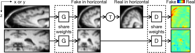
Figure 1: Flowchart of our algorithm. The generator blurs and downsamples the horizontal direction of an extracted image patch, and the discriminator determines whether the horizontal direction of the input is fake or real LR and outputs a “pixel-wise” probability map. G: generator; D: discriminator; T: transpose.

We regard the 3D object, $f$, imaged in a MR scanner, as being represented by the continuous function $f(x,y,z)$. We model the slice selections and signal excitation in a multi-slice 2D acquisition as a convolution between $f$ and the 1D PSF $p_{l}(z)$,

$$f(x,y,z)\ast_{z}p_{l}(z).$$

We use $\ast_{z}$ to denote the 1D convolution along the $z$-axis, since the symbol $\ast$ generally represents the 3D convolution along $x$-, $y$-, and $z$-axes. We assume that the truncated k-space sampling imposes two 1D PSFs $p_{h}(x)$ and $p_{h}(y)$, which are identical to each other but operate on different axes, onto the $xy$-plane,

$$f(x,y,z)\ast_{z}p_{l}(z)\ast_{x}p_{h}(x)\ast_{y}p_{h}(y),$$

where $\ast_{x}$ and $\ast_{y}$ denote the 1D convolutions along the $x$- and $y$-axes, respectively. In general, the in-plane—the $xy$-plane in this case—resolution is higher than the through-plane—the $z$-axis—resolution. This indicates that $p_{h}$ (usually) has a smaller FWHM than $p_{l}$. Additionally, the acquisition of an image also includes sampling or digitization. In this work, we represent this as,

$$\left\{f\ast_{z}p_{l}\ast_{x}p_{h}\ast_{y}p_{h}\right\}\downarrow_{(s_{z},s_{x},s_{y})},$$ (1)

where $s_{x}$, $s_{y}$, and $s_{z}$ are sampling step sizes along the $x$-, $y$-, and $z$-axes, respectively. We further assume that $s_{x}=s_{y}<s_{z}$, which is the situation in a typical multi-slice 2D acquisition.

2.2 Slice Profile and Internal Patch Distributions

In medical imaging, we observe that $f$ can express similar patterns (without any blurring) along the $x$, $y$, and $z$ axes [18, 15]. We use the following notations,

$$I_{xz}=f(x,y,z)\mid_{(x,y,z)\in\Omega_{xz}}\quad\mathrm{and}\quad I_{zx}=f(x,y,z)\mid_{(x,y,z)\in\Omega_{zx}},$$

to denote 2D patches extracted from the $xz$- and $zx$-planes, respectively, where $\Omega_{xz}$ and $\Omega_{zx}$ are the corresponding coordinate domains of these 2D patches. It should be self-evident that the patches $I_{xz}$ and their transposes $I_{zx}$ can be assumed to follow the same distribution $\mathcal{F}$. That is,

$$I_{xz}\sim\mathcal{F}\quad\mathrm{and}\quad I_{zx}=I_{xz}^{T}\sim\mathcal{F}.$$

The self-similar phenomenon implies that the patches extracted from the $yz$- and $zy$-planes can also be assumed to follow $\mathcal{F}$. Without loss of generality, we restrict our exposition to the patches $I_{xz}$ and $I_{zx}$.

In a multi-slice 2D MR image, we cannot directly extract patches from $f$. Indeed, as noted in Eq. (1), the continuous $f$ is blurred by PSFs then sampled to form a digital image. Instead, we think of the sampled patches as,

$$I_{hl}=\left\{I_{xz}\ast_{1}p_{h}\ast_{2}p_{l}\right\}\downarrow_{(s_{x},s_{z})}\quad\mbox{ and }\quad I_{lh}=\left\{I_{zx}\ast_{1}p_{l}\ast_{2}p_{h}\right\}\downarrow_{(s_{z},s_{x})},$$ (2)

where $\ast_{1}$ and $\ast_{2}$ are 1D convolutions along the first and second dimensions of these patches, respectively, and $\downarrow_{(s_{x},s_{z})}$ represents the sampling along the first and second dimensions with factors $s_{x}$ and $s_{z}$, respectively. This can be summarized as saying that $I_{lh}$ is blurrier in its first dimension than its second dimension since $s_{z}>s_{x}$, and $p_{l}$ has a wider FHWM than $p_{h}$; in contrast, in $I_{hl}$, the second dimension is blurrier than its first dimension. Therefore, these two patches, $I_{lh}$ and $I_{hl}$, cannot be assumed to follow the same distribution anymore. All is not lost, however. Suppose that we know the difference between $p_{h}$ and $p_{l}$, which we express as another 1D function $k$, such that $p_{h}\ast k=p_{l}$, and the difference between the sampling rates $s_{x}$ and $s_{z}$, defined as $s=s_{z}/s_{x}$. In this case, we can use the self-similar phenomenon and make the following statements:

$$\left\{I_{hl}\ast_{1}k\right\}\downarrow_{(s,1)}\sim\mathcal{F^{\prime}}\qquad\mbox{ and }\qquad\left\{I_{lh}\ast_{2}k\right\}\downarrow_{(1,s)}\sim\mathcal{F^{\prime}},$$ (3)

where $\mathcal{F^{\prime}}$ is the resultant patch distribution. This indicates that after correctly blurring then downsampling each patch, these new patches should follow the same distribution, namely $\mathcal{F^{\prime}}$. We note that Eq. (3) only holds approximately; in general, convolution and downsampling operations do not commute.

Since $k$ is the difference of the through-plane slice profile $p_{l}$ from the in-plane HR PSF $p_{h}$, we call $k$ a “relative” slice profile. We argue that estimating $k$ should be sufficient for the task of improving supervised super-resolution since we only want to create training pairs from the HR image or patches that have already been blurred by $p_{h}$, and $p_{h}$ may or may not be known. Based on Eq. (3), we formulate the estimation of $k$ as a problem of internal patch distribution matching. This points us to using a GAN, which is capable of learning an image distribution during an image translation task.

2.3 Slice Profile and GAN

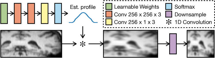
Figure 2: Architecture of our generator. A series of 1D convolutions, followed by softmax, outputs the estimated slice profile. An image patch is convoled with this slice profile then downsampled. Conv $\bm{C_{in}\times C_{out}\times W}$: 1D convolution along the horizontal dimension with the number of input channels $C_{in}$, the number of output channels $C_{out}$, and the size of the kernel $W$; Est. profile: the estimated slice profile.

According to our analysis in Sec. 2.2, we can estimate the relative slice profile $k$ by learning to match the internal patch distributions of a given image volume. In this work, we use a GAN to facilitate this process. In the following discussion, we directly use the term “slice profile” to refer to $k$ for simplicity.

The flowchart of our proposed algorithm is shown in Fig. 1. Suppose that the $xy$-axes are HR directions and the $z$-axis is LR. $xz$ or $yz$ patches are randomly extracted from the given image volume with sampling probabilities proportional to the image gradients. As shown in Fig. 1, our generator blurs and downsamples an input image patch only along the horizontal direction. If the generator output is transposed, its horizontal direction is the real LR from the image volume; if not transposed, it means that its horizontal direction is degraded by the generator. Therefore, we restrict the receptive field of our discriminator to be 1D, so it can only learn to distinguish the horizontal direction of the image patch.

2.3.1 Loss Function.

We updated the conventional GAN value function of the min-max equation [6] to accommodate our model in Eq. (3) as,

$$\min_{G}\max_{D}\left\{\mathbb{E}_{I}[\log D(G(I)^{T})]+\mathbb{E}_{I}[\log(1-D(G(I)))]\right\},$$ (4)

where $G$ is the generator, $D$ is the discriminator, $I$ is a 2D patch extracted from the image volume, and the superscript $T$ represents transpose. Since the first term in Eq. (4) includes the generator $G$, we include it in the generator loss function:

$$L_{adv}=\log D(G(I_{1})^{T})+\log(1-D(G(I_{2})))$$ (5)

to learn the generator, where $I_{1}$ and $I_{2}$ are two patches independently sampled from the image. In practice, since our $D$ outputs a pixel-wise probability map (see Fig. 3), we calculate $L_{adv}$ as the average across all pixels of a patch.

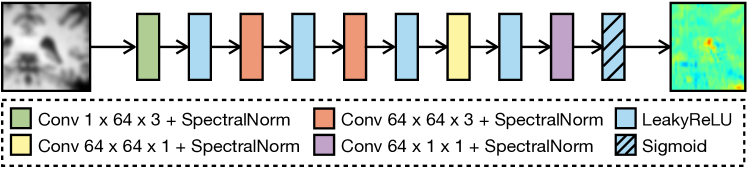
Figure 3: Architecture of our discriminator. This discriminator has a 1D horizontal receptive field and determines whether each pixel location horizontally corresponds to the real LR or is degraded by the generator. Conv $\bm{C_{in}\times C_{out}\times W}$: 1D convolution along the horizontal dimension with the number of input channels $C_{in}$, the number of output channels $C_{out}$, and the size of the kernel $W$; SpectralNorm: Spectral normalization.

2.3.2 Generator Architecture.

The architecture of our GAN generator is shown in Fig. 2. Different from previous methods [2, 5, 3], we do not take the image patch as the input to the generator network. Instead, we use the network to learn a 1D slice profile and convolve it with the patch (without padding). In this way, we can enforce the model in Eq. (3) and impose positivity and the property of sum-to-one for the slice profile using softmax. Similar to [2], we do not have non-linearity between convolutions. Additionally, we want the slice profile to be smooth. Inspired by the deep image prior [14, 4, 13], we note that this smoothness can be regarded as local correlations within the slice profile. We then use a learnable tensor (the green box in Fig. 2) as input to the generator network and simultaneously learn a series of convolution weights on top of it. In other words, we can capture the smoothness of the slice profile using only the network architecture. For this to work, we additionally incorporate an $l^{2}$ weight decay during the learning of this architecture, as suggested by [4].

2.3.3 Discriminator Architecture.

The architecture of the discriminator is shown in Fig. 3. To restrict its receptive field, we only use 1D convolutions (without padding) along the horizontal direction. The first three convolutions have kernel size 3, and the last two have kernel size 1. This is equivalent to a receptive field of 7, so the discriminator is forced to learn from local information. To stabilize GAN training, we adjust the convolution weights using spectral normalization [11] and use leaky ReLU with a negative slope equal to 0.1 in-between. This discriminator learns to distinguish whether the horizontal direction at each pixel is from the real LR or degraded by the generator; it outputs a “pixel-wise” probability map.

2.4 Regularization Functions and Other Details

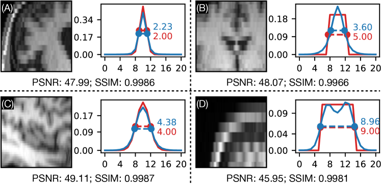
Figure 4: Example estimated slice profiles of the simulations. Image slices are shown partially with nearest neighbor upsampling for display purposes. True (red) and estimated (blue) slice profiles are shown with their corresponding FWHMs. (A): FWHM = 2 mm, scale factor = 4; (B): FWHM = 5 mm, scale factor = 4; (C): FWHM = 4mm, scale factor = 2; (D): FWHM = 9, scale factor = 8.

In addition to our adversarial loss in Eq. (5), we use the following losses to regularize the slice profile $k$:

$$L_{c}=\left(\sum_{i=0}^{K-1}{ik_{i}}-\lfloor K/2\rfloor\right)^{2}\quad\mathrm{and}\quad L_{b}=k_{0}+k_{1}+k_{K-1}+k_{K-2},$$

where $K$ is the length of $k$ and $\lfloor.\rfloor$ is the floor operation. $L_{c}$ encourages the centroid of $k$ to align with the central coordinate, and $L_{b}$ encourages its borders to be zero [2]. Note that our $k$ is guaranteed to be positive and sum to one due to the use of softmax (Fig 2). Therefore, our total loss for the generator is

$$L=L_{adv}+\lambda_{c}L_{c}+\lambda_{b}L_{b}+\lambda_{w}WD,$$

where $WD$ is $l^{2}$ weight decay, and $\lambda_{c}=1$, $\lambda_{b}=10$, and $\lambda_{w}=0.05$ are the corresponding loss weights, determined empirically. Inspired by [17], we further use exponential moving average $\bar{k}$ as our result to stabilize the estimation,

$$\bar{k}^{(t)}=\beta\bar{k}^{(t-1)}+(1-\beta)k^{(t)},$$

where $t$ is the index of the current iteration, and $\beta=0.99$. We use two separate Adam optimizers [7] for the generator and the discriminator, respectively, with parameters learning rate $=2\times 10^{-4}$, $\beta_{1}=0.5$, and $\beta_{2}=0.999$. Unlike the generator, the optimizer of the discriminator does not have weight decay, and the generator optimizer also has gradient clipping. The number of iterations is 15,000 with a mini-batch size of 64. The size of an image patch is 16 along the LR direction, and we make sure that after the generator, the HR direction also has size 16. We initialize the slice profile to be an impulse function before training.

Table 1: Errors between true and estimated profiles in the simulations with Gaussian and rect profiles. The mean values across five subjects are shown for each metric. F. err.: absolute error between FWHMs; P. err.: sum of absolute errors between profiles.

Gaussian profile
FWHM	2 mm			4 mm			8 mm
Scale	2	4	8	2	4	8	2	4	8
F. Err.	0.32	0.41	0.69	0.36	0.26	0.52	0.97	0.23	1.33
P. Err.	0.20	0.23	0.33	0.11	0.11	0.13	0.10	0.09	0.23
PSNR	46.68	45.80	42.81	50.34	51.45	51.46	50.26	55.43	46.93
SSIM	0.9976	0.9974	0.9957	0.9987	0.9991	0.9993	0.9982	0.9994	0.9975
Rect profile
FWHM	3 mm			5 mm			9 mm
Scale	2	4	8	2	4	8	2	4	8
F. Err	0.55	0.62	0.35	0.06	1.54	1.98	0.18	0.53	0.46
P. Err	0.44	0.44	0.47	0.28	0.41	0.45	0.25	0.24	0.23
PSNR	45.89	46.01	43.43	47.02	46.25	45.19	46.92	50.47	48.77
SSIM	0.9971	0.9976	0.9963	0.9973	0.9972	0.9971	0.9960	0.9987	0.9986

3 Experiments and Results

3.1 Simulations from Isotropic Images

In the first experiment to test the proposed algorithm, we simulated LR images from isotropic brain scans of five subjects from the OASIS-3 dataset [8]. These images are scanned using the magnetization prepared rapid acquisition gradient echo (MPRAGE) sequence with a resolution of 1 mm. We generated two types of 1D functions, Gaussian and rect, to blur the through-plane direction of these images. The Gaussian functions have FWHMs of 2, 4, and 8 mm, and the rect functions have FWHMs of 3, 5, and 9 mm. After blurring, we downsampled these images with scale factors of 2, 4, and 8. As a result, we generated $2\times 3\times 3=18$ types of simulations for each of the five subjects. We then ran our algorithm on all these simulated images. Four metrics were used to evaluate the estimated profiles: the absolute error between the FWHMs of true and estimated profiles (FHWM error), the sum of absolute errors between the true and estimated profiles (profile error), and peak signal-to-noise ratio (PSNR) and structural similarity (SSIM) between the images degraded by the true and estimated profiles. Note that we calculate SSIM and PSNR within a head mask. We show these results in Table 1. Example images and slice profiles are shown in Fig. 4. Despite high FHWM and profile errors, we observe that the PSNR and SSIM results are very good. We attribute this disparity to the ill-posed nature of the problem, as different slice profiles can generate very similar LR images.

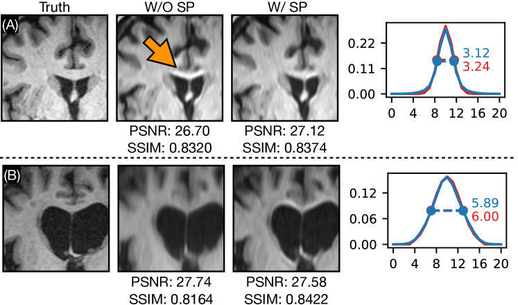
Figure 5: SMORE results. Image slices are shown partially for display purposes. True (red) and estimated (blue) profiles are shown with their corresponding FWHMs. The arrow points to an artifact. Row (A): FWHM = 3.2 mm, scale factor = 4; Row (B): FWHM = 6.0 mm, scale factor = 4. W/O SP, W/ SP: without and with incorporating our estimate of the profile into SMORE, respectively.

Table 2: SSIM and PSNR between SMORE results and the true HR images with and without using the estimated slice profiles. Each metric is shown as the mean across five subjects. W/ SP: incorporating our estimate of slice profile.

FWHM	2.0 mm		3.2 mm		4.8 mm		6.0 mm
W/ SP	False	True	False	True	False	True	False	True
PSNR	26.11	27.81	27.57	27.86	28.57	27.78	28.15	27.79
SSIM	0.8223	0.8517	0.8523	0.8558	0.8570	0.8565	0.8343	0.8540

3.2 Incorporating Slice Profile Estimation Into SMORE

SMORE [18] is a self-supervised (without external training data) super-resolution algorithm to improve the through-plane resolution of multi-slice 2D MR images. It does not know the slice profile and assumes it is a 1D Gaussian function with FWHM equal to the slice separation. In this experiment, we incorporated our algorithm into SMORE and compared the performance difference with and without our estimated slice profiles. Throughout this work, we trained SMORE from scratch for 8,000 iterations. We simulated low through-plane resolution images from our five OASIS-3 scans. We used only Gaussian functions to blur these images with a scale factor of 4. The Gaussian functions have FWHMs of 2, 3.2, 4.8, and 6 mm. Therefore, we generated 4 simulations for each of the five scans. When not knowing the slice profile, we assume it is a Gaussian function with FWHM = 4 mm (which is the slice separation in our simulations). After running SMORE, we calculated the PSNR and SSIM between the SMORE results and the true HR images as shown in Table 2. Example SMORE results with and without knowing the estimated slice profiles are shown in Fig. 5. Table 2 shows better PSNR and SSIM, if our estimated profiles are used, for simulations with FWHMs of 2 and 3.2 mm. The PSNR are worse for 4.8 and 6.0 mm, but SSIM is better for FWHM 6.0 mm.

3.3 Measuring Through-Plane Resolution After Applying SMORE

In this experiment, we use the FWHMs of our estimated slice profiles to measure the resultant resolution after applying SMORE to an image. We used Gaussian functions to blur the five OASIS-3 scans. The first type (Type 1) of simulations has a FWHM of 2 mm and a scale factor of 2, while the second type (Type 2) has FWHM of 4 mm and a slice factor of 4. We first used SMORE to super-resolve these images then applied our slice profile estimation to measure resultant through-plane resolution. Type 1 has mean FWHM = 1.9273 mm with standard deviation (SD) = 0.0583 mm across the five subjects. Type 2 has mean FWHM = 2.9044 mm with SD = 0.1553 mm. Example SMORE results and resolution measurements are shown in Fig. 6.

4 Discussion and Conclusions

In this work, we proposed to estimate slice profiles of multi-slice 2D MR images by learning to match the internal patch distributions. Specifically, we argue that if an HR in-plane direction is degraded by the correct slice profile, the distribution of patches extracted from this direction should match the distribution of patches extracted from the LR through-plane direction. We then proposed to use a GAN to learn the slice profile as a part of the generator. Our algorithm is validated using numerical simulations and incorporated into SMORE to improve its super-resolution results. We further show that our algorithm is also capable of measuring through-plane resolution.

The first limitation of our algorithm is that it is unable to learn a slice profile with a flexible shape as shown in Fig. 4, where the true profiles are rect functions. This is because we used a similar generator architecture as the deep image prior to encourage smoothness. We found that the value of $\lambda_{w}$ for weight decay greatly affected the performance. Specifically, with a small $\lambda_{w}$, the shape of the learned slice profile is more flexible, but the training is very unstable and can even diverge. A better way to regularize the slice profile should be investigated in the future.

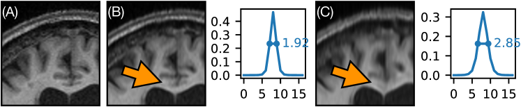
Figure 6: Resolution measurements of super-resolved images. SMORE results and the corresponding slice profile estimates from the resultant images of SMORE are shown in (B) and (C). The FWHMs of estimated profiles are marked on the side. The arrows point to the differences. (A): truth HR image; (B): SMORE result from a simulation with FWHM = 2 mm; (C): SMORE result from a simulation with FWHM = 4 mm.

The second limitation is our inconclusive improvement to the SMORE algorithm. Indeed, we have better PSNR and SSIM when the slice thickness is smaller than the slice separation (resulting in slice gaps when FWHMs are 2 and 3.2 mm in Table 2); this does not seem to be the case when the slice thickness is larger (resulting in slice overlaps when FWHMs are 4.8 and 6.0 mm in Table 2). We regard this as a counter-intuitive result and plan to conduct more experiments with SMORE, such as train with more iterations, and testing other super-resolution algorithms.

5 Acknowledgments

This work was supported by a 2019 Johns Hopkins Discovery Award and NMSS Grant RG-1907-34570.

References

- [1] American College of Radiology Magnetic Resonance Imaging Accreditation Program: Phantom Test guidance for use of the large MRI phantom for the ACR MRI accreditation program, p. 16 (2018), https://www.acraccreditation.org/-/media/ACRAccreditation/Documents/MRI/LargePhantomGuidance.pdf
- [2] Bell-Kligler, S., Shocher, A., Irani, M.: Blind super-resolution kernel estimation using an internal-GAN. In: Advances in Neural Information Processing Systems 32, pp. 284–293. Curran Associates, Inc. (2019)
- [3] Chen, S., Han, Z., Dai, E., Jia, X., Liu, Z., Xing, L., Zou, X., Xu, C., Liu, J., Tian, Q.: Unsupervised image super-resolution with an indirect supervised path. In: Proceedings of the IEEE/CVF Conference on Computer Vision and Pattern Recognition Workshops (2020)
- [4] Cheng, Z., Gadelha, M., Maji, S., Sheldon, D.: A Bayesian perspective on the deep image prior. In: Proceedings of the IEEE/CVF Conference on Computer Vision and Pattern Recognition (2019)
- [5] Deng, S., Fu, X., Xiong, Z., Chen, C., Liu, D., Chen, X., Ling, Q., Wu, F.: Isotropic reconstruction of 3D EM images with unsupervised degradation learning. In: 23 International Conference on Medical Image Computing and Computer Assisted Intervention. pp. 163–173. Springer International Publishing, Cham (2020)
- [6] Goodfellow, I., Pouget-Abadie, J., Mirza, M., Xu, B., Warde-Farley, D., Ozair, S., Courville, A., Bengio, Y.: Generative adversarial nets. In: Advances in Neural Information Processing Systems 27. pp. 2672–2680. Curran Associates, Inc. (2014)
- [7] Kingma, D.P., Ba, J.: Adam: A method for stochastic optimization. arXiv preprint: 1412.6980 (2017)
- [8] LaMontagne, P.J., Benzinger, T.L., Morris, J.C., Keefe, S., Hornbeck, R., Xiong, C., Grant, E., Hassenstab, J., Moulder, K., Vlassenko, A.G., Raichle, M.E., Cruchaga, C., Marcus, D.: OASIS-3: Longitudinal neuroimaging, clinical, and cognitive dataset for normal aging and Alzheimer disease. medRxiv (2019)
- [9] Lerski, R.A.: An evaluation using computer simulation of two methods of slice profile determination in MRI. Physics in Medicine and Biology 34(12), 1931–1937 (1989)
- [10] Liu, H., Michel, E., Casey, S.O., Truwit, C.L.: Actual imaging slice profile of 2D MRI. In: Medical Imaging 2002: Physics of Medical Imaging. vol. 4682, pp. 767 – 773. SPIE (2002)
- [11] Miyato, T., Kataoka, T., Koyama, M., Yoshida, Y.: Spectral normalization for generative adversarial networks. In: International Conference on Learning Representations (2018)
- [12] Prince, J.L., Links, J.M.: Medical imaging signals and systems. Upper Saddle River, N.J.: Pearson Prentice Hall (2006)
- [13] Ren, D., Zhang, K., Wang, Q., Hu, Q., Zuo, W.: Neural blind deconvolution using deep priors. In: Proceedings of the IEEE/CVF Conference on Computer Vision and Pattern Recognition (2020)
- [14] Ulyanov, D., Vedaldi, A., Lempitsky, V.: Deep image prior. In: Proceedings of the IEEE/CVF Conference on Computer Vision and Pattern Recognition (2018)
- [15] Weigert, M., Royer, L., Jug, F., Myers, G.: Isotropic reconstruction of 3D fluorescence microscopy images using convolutional neural networks. In: 20 International Conference on Medical Image Computing and Computer Assisted Intervention. pp. 126–134. Springer International Publishing, Cham (2017)
- [16] Xuan, K., Si, L., Zhang, L., Xue, Z., Jiao, Y., Yao, W., Shen, D., Wu, D., Wang, Q.: Reduce slice spacing of MR images by super-resolution learned without ground-truth. arXiv preprint: 2003.12627 (2020)
- [17] Yazıcı, Y., Foo, C., Winkler, S., Yap, K., Piliouras, G., Chandrasekhar, V.: The unusual effectiveness of averaging in GAN training. In: International Conference on Learning Representations (2019)
- [18] Zhao, C., Carass, A., Dewey, B.E., Woo, J., Oh, J., Calabresi, P.A., Reich, D.S., Sati, P., Pham, D.L., Prince, J.L.: A deep learning based anti-aliasing self super-resolution algorithm for MRI. In: 21 International Conference on Medical Image Computing and Computer Assisted Intervention. pp. 100–108. Springer (2018)
- [19] Zhao, C., Shao, M., Carass, A., Li, H., Dewey, B.E., Ellingsen, L.M., Woo, J., Guttman, M.A., Blitz, A.M., Stone, M., Calabresi, P.A., Halperin, H., Prince, J.L.: Applications of a deep learning method for anti-aliasing and super-resolution in MRI. Magnetic Resonance Imaging 64, 132–141 (2019)