Eulerian simulation of complex suspensions and biolocomotion in three dimensions

Abstract

We present a numerical method specifically designed for simulating three-dimensional fluid–structure interaction (FSI) problems based on the reference map technique (RMT). The RMT is a fully Eulerian FSI numerical method that allows fluids and large-deformation elastic solids to be represented on a single fixed computational grid. This eliminates the need for meshing complex geometries typical in other FSI approaches, and greatly simplifies the coupling between fluid and solids. We develop the first three-dimensional implementation of the RMT, parallelized using the distributed memory paradigm, to simulate incompressible FSI with neo-Hookean solids. As part of our new method, we develop a new field extrapolation scheme that works efficiently in parallel. Through representative examples, we demonstrate the method’s accuracy and convergence, as well as its suitability in investigating many-body and active systems. The examples include settling of a mixture of heavy and buoyant soft ellipsoids, lid-driven cavity flow containing a soft sphere, and swimmers actuated via active stress.

Introduction

Fluid–structure interactions (FSI) are at the heart of many important physical and biological problems, including flexible structures in flow [1, 2], blood circulation in the heart [3, 4], animal locomotion [5, 6], and cilia motion [7, 8]. The couplings between fluid and immersed solids give rise to complex nonlinear dynamics dependent on geometry and boundary conditions, material constitutive relations, and collective interactions among the solid objects. Thus analytical solutions are rare and limited to simplified settings in reduced dimensions, and numerical methods for FSI have become indispensable for understand these problems.

In designing numerical methods for fluids and solids, Eulerian and Lagrangian perspectives are the more convenient choices, respectively, due to the differences in constitutive responses. Bridging between the two perspectives is a classic dilemma in developing numerical methods for FSI. Various frameworks have been proposed to resolve this dilemma. The immersed boundary method [3, 9] and the family of immersed methods that it inspires [4, 10, 11] solve fluid on a fixed mesh, use Lagrangian points to represent the solid, and employ a coupling scheme between the two. Arbitrary Lagrangian–Eulerian methods use moving nodes for both phases, and reposition the nodes to maintain mesh quality [12, 13].

There are also fully Eulerian methods, for which two types of formulations exist. The hypoelasticity formulation [14, 15, 16] uses linear elasticity, whereas the hyperelasticity formulation employs a general large-deformation description in the solids. To compute solid stresses in hyperelasticity, a variety of quantities have been used, such as level-set functions defining the fluid–solid interface [17], the deformation gradient tensor [18], the deformation tensors [19], and the solid displacements in the undeformed configuration [20, 21, 22].

The reference map technique (RMT) is a fully Eulerian approach that uses the solid’s reference coordinates as the primary simulation variables. The RMT has many favorable properties, and can simulate compressible fluid and solids [23, 24], handle contact between multiple solids [25], and simulate incompressible fluid and solids with complex geometries and actuation [26]. The RMT makes use of the level-set method [27, 28] for tracking the fluid–solid interfaces, and all prior versions have employed level-set reinitialization using the fast marching method (FMM) [28, 16]. Furthermore the FMM is used to extrapolate field values near the fluid–solid interface, which is a necessary part of the RMT.

All prior papers have demonstrated the method in two dimensions, yet a major strength of the fully Eulerian approach is the ability to avoid computational meshing of complex geometries, which becomes a compelling advantage in three dimensions (3D). Here, we provide the first 3D implementation of the RMT, and use it to simulate several scenarios that would be difficult do with existing numerical approaches. Inspired by recent work on fluid-filled soft granular packings [29], we simulate a suspension of soft flexible particles, half of which are lighter and half of which are heavier than the fluid. There has also been substantial recent interest in swimming and biolocomotion, yet reduced-dimension models of the swimmer [30, 31, 32] are often the state of the art. We demonstrate a model of a swimming organism using full volumetric actuation, creating a simulation tool that can explore a broader range of swimming modalities.

3D calculations are considerably more computationally challenging than two-dimensional (2D) ones, and we therefore present the first complete parallel implementation of the method using domain decomposition. Since the RMT uses a single fixed regular grid for fluid and solid, it is well-suited to parallelization, and different processors can each handle a rectangular subdomain. In addition, the regular grid structure makes contact among solid bodies easy to detect and allows for efficient memory storage. One challenge that we faced is that the FMM is not well-suited for parallelization, since it updates field values sequentially. We therefore a developed new method for extrapolation that can be done in parallel. Our new method removes the need for level-set reinitialization and fast marching methods, and the RMT implementation is therefore simplified from all prior approaches.

Theory and numerical method

Hyperelastic formulation

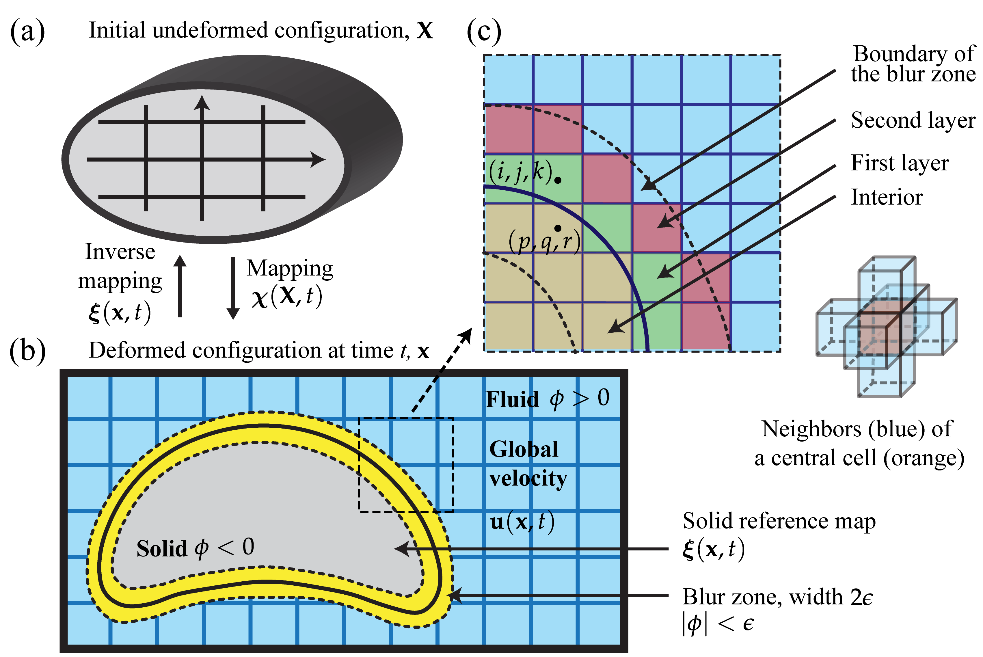
Figure 1: (a) An initially undeformed solid with reference configuration $\mathbf{X}$ undergoes a time-dependent mapping $\boldsymbol{\chi}(\mathbf{X},t)$ to its current configuration at time $t$. (b) A level-set function $\phi(\mathbf{x},t)$ distinguishes the two phases which share a global velocity $\mathbf{u}(\mathbf{x},t)$. A blur zone (yellow), defined by $|\phi|<\epsilon$, is used to transition between phases. (c) The order in which $\boldsymbol{\xi}(\mathbf{x},t)$ is extrapolated is defined by layers. The $1^{\text{st}}$ layer (green), e.g. cell $(i,j,k)$, are non-interior orthogonal neighbors to the interior cells (yellow), e.g. cell $(p,q,r)$. Subsequent layers, e.g. $2^{\text{nd}}$ layers (red), are constructed in the same way, until the blur zone is filled or a physical boundary is reached. 2D schematics are shown for clarity.

In the hyperelasticity framework [33], a time-dependent mapping function $\boldsymbol{\chi}(\mathbf{X},t)$ is introduced to determine how the undeformed configuration, $\mathbf{X}$, is transformed to its current physical configuration, $\mathbf{x}$, i.e. $\mathbf{x}=\boldsymbol{\chi}(\mathbf{X},t)$ (Fig. 1(a, b)). The deformation gradient is defined as $\mathbf{F}=\tfrac{\partial\boldsymbol{\chi}}{\partial\mathbf{X}}=\tfrac{\partial\mathbf{x}}{\partial\mathbf{X}}$. A constitutive relation $\boldsymbol{\sigma}_{s}(\mathbf{F})$ defines the Cauchy stress response in the solid material. The solid momentum balance equation in rate form is

$$\rho_{s}\left(\frac{\partial\mathbf{u}}{\partial t}+(\mathbf{u}\cdot\nabla)\mathbf{u}\right)=\nabla\cdot\boldsymbol{\sigma}_{s}$$ (1)

where $\rho_{s}$ is the solid density and $\mathbf{u}$ is the solid velocity. For an incompressible material $\det\mathbf{F}=1$ and thus solid density is unaffected by the deformation. To proceed, we assume that $\boldsymbol{\chi}$ is a sufficiently smooth function of $\mathbf{X}$ and $t$ and define its inverse as the reference map, $\mathbf{X}=\boldsymbol{\xi}(\mathbf{x},t)=\boldsymbol{\chi}^{-1}(\mathbf{x},t)$. The deformation gradient tensor becomes

$$\mathbf{F}=\left(\tfrac{\partial\boldsymbol{\xi}}{\partial\mathbf{x}}\right)^{-1}=\left(\mathbf{\nabla}_{\mathbf{x}}\boldsymbol{\xi}\right)^{-1}$$ (2)

where $\mathbf{\nabla}_{\mathbf{x}}$ is the gradient operator in physical space. The reference configuration is constant, therefore $\dot{\boldsymbol{\xi}}(\mathbf{x},t)=\mathbf{0}$, i.e.,

$$\frac{\partial\boldsymbol{\xi}}{\partial t}+(\mathbf{u}\cdot\nabla)\boldsymbol{\xi}=\mathbf{0}.$$ (3)

We discuss coupling fluid and solid phases and imposing the incompressibility constraint next.

Blurred interface method and monolithic governing equations

Consider a domain $\Omega$ containing $n$ immersed solid objects covering subdomains $\Omega_{1},\ldots,\Omega_{n}$. Denote the fluid domain as $\Omega_{f}$ and the solid domain $\Omega_{s}=\cup_{k=1}^{n}\Omega_{k}$ for $k=1,2,\ldots,n$, so that $\Omega=\Omega_{s}\cup\Omega_{f}$. The fluid–solid interface (hereinafter the interface) is denoted as $\partial\Omega_{s}=\cup_{k=1}^{n}\partial\Omega_{k}$ for $k=1,2,\ldots,n$. To avoid excessive distortion, the reference map $\boldsymbol{\xi}$ is only defined and evolved within $\Omega_{s}$. The solution to Eq. (3) is the union of solutions within each $\Omega_{k}$. The velocity $\mathbf{u}$ is defined as a global variable spanning $\Omega$. The incompressibility constraint implies that

$$\nabla\cdot\mathbf{u}=0$$ (4)

in $\Omega$. To enforce the constraint, a global pressure field is used as a Lagrange multiplier. Thus, we need only consider the deviatoric part of the stress tensors. For the fluid, we consider the deviatoric stress of a viscous Newtonian fluid, $\boldsymbol{\tau}_{f}=\mu\left(\nabla\mathbf{u}+\nabla\mathbf{u}^{\mathsf{T}}\right)$, where $\mu$ is the fluid dynamic viscosity. The deviatoric solid stress is defined as $\boldsymbol{\tau}_{s}=\boldsymbol{\sigma}_{s}-\tfrac{1}{3}\operatorname{tr}(\boldsymbol{\sigma}_{s})\mathbf{1}$.

In a physical system, there may be discontinuities in velocity, density, stresses, and forces across the interface. In our method, we consider a continuous velocity field, which naturally corresponds to a no-slip boundary condition at $\partial\Omega_{s}$. Next, we discuss the blurred interface method that ensures the traction-matching condition, i.e. $\boldsymbol{\sigma}_{s}\cdot\mathbf{n}=\boldsymbol{\sigma}_{f}\cdot\mathbf{n}$, is satisfied at the interface, and creates a smooth transition of field values across the interface.

The basic RMT equations work with a variety of interfacial coupling procedures, including sharp and blurred interface methods [24, 25, 26]. In this work we focus on a blurred interface method because it has several advantages over a sharp interface method, e.g., it is more stable to interfacial perturbations, more amenable to simulating immersed solid–solid contact, and easier to implement [25, 26]. Continuing with the blurred interface method, we make use of a blur zone of width $2\epsilon$ across the interface. The width of the blur zone $2\epsilon$ scales with the grid spacing so that as grid spacing approaches zero, a sharp interface representation is recovered. Without loss of generality, we consider a single solid object with interface $\partial\Omega_{s}$ defined by the zero contour of a signed-distance function in the undeformed configuration, $\phi_{0}(\mathbf{X})$. Throughout the simulation, we define the time-dependent level-set function $\phi(\mathbf{x},t)=\phi_{0}(\boldsymbol{\xi}(\mathbf{x},t))$ (Fig. 1(b)).

In the blur zone, quantities that may have jump across the interface, e.g. $\rho$, $\boldsymbol{\tau}$ and $\mathbf{b}$, are blended to smoothly vary between the fluid and the solid phases [34, 35, 36]. Let $Q$ denote a scalar, or a component of a vector or a tensorial quantity in $\Omega$. Consider $Q_{f}$ in the fluid domain $\Omega_{f}$, and $Q_{s}$ in the solid domain $\Omega_{k}$. We blend $Q_{f}$ and $Q_{s}$ such that $Q$ transitions smoothly between $\Omega_{f}$ and $\Omega_{k}$,

$$Q=Q_{s}+H_{\epsilon}(\phi)(Q_{f}-Q_{s})$$ (5)

where $\phi$ is the value of the level-set function defining the boundary of $\Omega_{k}$, and $H_{\epsilon}(\phi)$ is a smoothed Heaviside function,

$$H_{\epsilon}(\phi)=\left\{\begin{array}[]{ll}0&\qquad\text{if $\phi\leq-\epsilon$,}\\ \frac{1}{2}(1+\frac{\phi}{\epsilon}+\frac{1}{\pi}\sin\frac{\pi\phi}{\epsilon})&\qquad\text{if $|\phi|<\epsilon$,}\\ 1&\qquad\text{if $\phi\geq\epsilon$},\end{array}\right.$$ (6)

which has a continuous second derivative. The momentum balance equation of the coupled fluid–structure system is

$$\rho\left(\frac{\partial\mathbf{u}}{\partial t}+(\mathbf{u}\cdot\nabla)\mathbf{u}\right)=-\nabla p+\nabla\cdot\boldsymbol{\tau}+\mathbf{b}$$ (7)

with blended $\rho$, $\boldsymbol{\tau}$, and $\mathbf{b}$. The monolithic equation above satisfies the flow equation and elasticity equation, in the fluid and the solid phases, respectively. Furthermore, the traction-matching condition is also automatically satisfied due to blending of stresses near the interface. Eqs. (3), (4), & (7) form a single set of governing equations for the coupled FSI system.

In the solid bodies, we add an artificial viscosity $\mu_{a}$ to improve numerical stability. If $\mu_{a}$ scales with grid size, in the limit of very fine spatial resolution, we recover the undamped solid equation. If it is set to a grid size-independent constant, it is equivalent to simulating a Kelvin–Voigt viscoelastic solid. We also define a dimensionless constant $\gamma_{t}$ that applies an additional multiplicative factor to the artificial viscosity in the blur zone (see SI for details).

Extrapolation of $\boldsymbol{\xi}(\mathbf{x},t)$

Since $\boldsymbol{\xi}(\mathbf{x},t)$ is only defined inside the solid, it needs to be extrapolated to several grid cells outside of the interface for calculating derivatives in Eq. (3) and the deformation gradient tensor $\mathbf{F}$ near the interface. We describe our new extrapolation method for a single solid occupying domain $\Omega_{s}$, though it can be easily applied to any number of objects. First we simplify the spatial order in which $\boldsymbol{\xi}(\mathbf{x},t)$ is extrapolated by making use of adjacency rules on a fixed grid. Consider a Cartesian mesh with $M\times N\times O$ grid cells indexed by $i,j,k$, we define orthogonal neighbors of a central cell as those cells that share a common face with the central cell (Fig. 1(c)). We label cells with $\phi<0$ as the interior cells, or equivalently, as cells in the zeroth layer. All the other cells are left as unmarked. Then, for each interior cell, we label its unmarked orthogonal neighbors as the first layer cells, with index $l=1$. We repeat this procedure to find subsequent layers $l=2,3,\ldots$, until we reach a physical boundary or the maximum number of layers, whichever occurs earlier. The maximum number of layers is chosen so that the entire blue zone can be covered by the extrapolation procedure while conserving computational resources.

The extrapolation is then performed in ascending order of layers, but it can be computed independently for each cell within the same layer. Suppose we aim to create an extrapolated reference map, $\boldsymbol{\xi}_{e}=(\xi_{i},\xi_{j},\xi_{k})$ in layer $l_{i,j,k}$, with cell index $(i,j,k)$. Subscript $e$ denotes an extrapolated cell. Using WLS regression, we first build a local linear model of the reference map $\boldsymbol{\xi}(\mathbf{x},t)$ as a function of physical coordinate $\mathbf{x}$. To find eligible data points for the regression, we search within a $r_{s}=2$ box centered at cell $(i,j,k)$, where $r_{s}$ is the search radius measured in number of grid cells. Consider a cell with index $(p,q,r)$ with $\boldsymbol{\xi}_{d}=(\xi_{p},\xi_{q},\xi_{r})$, where subscript $d$ denotes a data cell. It is eligible to be a data point in the regression only if it is marked as a layer in the previous procedure, and $l_{p,q,r}<l_{i,j,k}$. In other words, reference map $\boldsymbol{\xi}_{d}$ must exist and be in layers lower than that of $\boldsymbol{\xi}_{e}$. In the case of multiple solid objects, $\boldsymbol{\xi}_{d}$ must emanate from the same object whose extrapolation we seek.

The weights in the regression are important to ensure the quality of the extrapolated values, especially when local deformations are large. In the weighting scheme, we use an exponential decaying kernel centered at the extrapolated cell, and near the interface we incorporate geometric information via $\phi_{0}$. Details are provided in the SI. The WLS problem is solved to obtain a set of coefficients $\boldsymbol{\beta}$, and extrapolated reference map is calculated by $\boldsymbol{\xi}_{e}(\mathbf{x}_{e},t)=\boldsymbol{\beta}\mathbf{x}_{e}$. If the linear system is degenerate, we increase the search radius $r_{s}$ by 1 and repeat the procedure from searching for eligible data points, but this is rare in practice.

In multi-body simulations, the extrapolation procedure is applied to each object independently. We require that solid bodies do not co-exist at a grid cell. However, the blur zone of an object is allowed to overlap with blur zones or interiors of other objects. Thus, at a single grid cell, there can be several reference maps, extrapolated or not, each belonging to a distinct object. Since extrapolated values are only needed in a small region near the interface, we design a custom data structure that is tailored to store these extrapolated values efficiently in memory. Besides eliminating the need of reinitialization, the current extrapolation method has two additional advantages: (1) layers can be defined given a definition of adjacency on the grid; (2) the method is layer-wise and object-wise independent, thus easy to be parallelized.

Numerical procedures and implementation

The RMT implementation in 3D (RMT3D) is developed in C++ and parallelized via domain decomposition using the Message-Passing Interface (MPI) library. The numerical schemes extend our previous work on 2D RMT implementation [26] and follow established discretizations for solving hyperbolic conservative laws [37, 36]. In summary, we extend from previous works the variable arrangement on the grid, finite-difference schemes to compute spatial derivatives, and Godunov-type upwinding scheme for hyperbolic conservation laws [38] to handle the advective parts of Eqs. (3) & (7). In addition, an approximate projection method [37, 39] and a marker-and-cell projection method are used to enforce the incompressibility constraint (Eq. (4)) on the velocity solution at each timestep, and on an intermediate velocity field between two timesteps, respectively. Large linear systems from the projection methods are solved using a custom geometric multigrid solver. In many-body simulations, a collision stress-based contact model developed in the previous work [26] is used. Details of the numerical schemes and convergence tests are provided in the SI.

Results

In this section, we consider immersed viscoelastic neo-Hookean solids (constant $\mu_{a}$) in various settings. We nondimensionalize the governing equations using appropriate length, time, and mass scales in each test case. We also use isotropic grid spacing $h$ in all simulations.

Settling sphere in a square cylinder

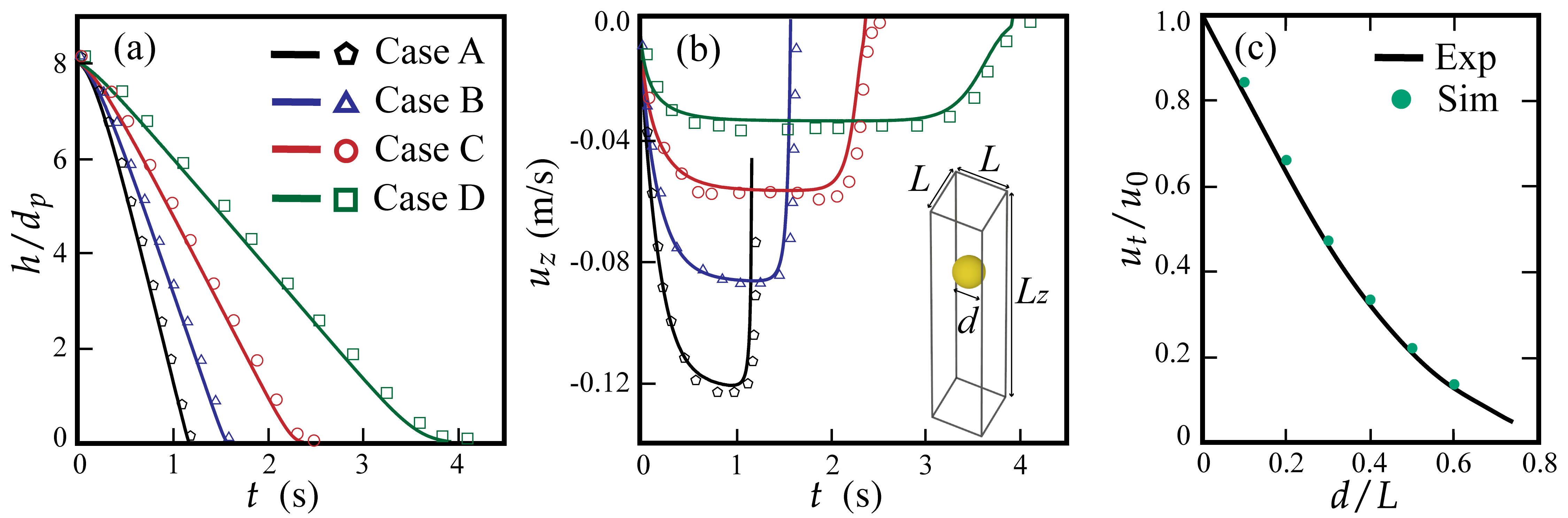
Figure 2: Comparisons of settling sphere simulations against experiments. The positions (a) and velocities (b) of a simulated sphere (solid lines) are compared with experimental results (symbols) by ten Cate et al. [40]. Parameters are given in Table 1. The inset in (b) shows an example simulation. (c) The wall correction factors in simulations are compared against experimental results by Miyamura et al. [41], using parameters $(L,L_{z},\rho_{s},\rho_{f},G,\mu,\mu_{a},\gamma_{t},h,\epsilon)=(1,6,2,1,10,0.04714,0.04714,0,1/160,1/320)$. Actual $\textit{Re}_{p}=0.021,$ $0.132,$ $0.319,$ $0.537,$ $0.694,$ $0.743,$ respectively, for spheres with increasing diameters.

The transport of rigid and deformable particles in fluid flow is central in many biological and physical systems. While analytical solutions are available for simple cases such as a rigid sphere in unbound creeping flow, more complex FSIs in this setting elude analytical approaches. In recent decades, the effects of confinement and multi-body interactions during settling have been a focus of much experimental and numerical work [41, 40, 42, 43, 44, 45]. In this section, we simulate a solid sphere with a high shear modulus settling in a confined geometry. We aim to demonstrate that by simply increasing the solid shear modulus, our method can easily capture the dynamics of a settling rigid sphere at various Reynolds number.

We compare simulated data with experimental measurements of positions, velocities, and wall correction factors on the terminal velocity of a rigid sphere settling in a square cylinder [40, 41]. We devise a dimensionless parameter $\zeta\equiv\rho_{f}Gd/(\rho_{s}\mu u_{0})$ that compares the strength of the solid elastic stress against that of the viscous stress, $u_{0}$ is the terminal velocity of a sphere in an unbound creeping flow, $G$ is the shear modulus, and $d$ is the sphere diameter. We find that a moderate value of $G$, much smaller than the experimental values, suffices to satisfy $\zeta\gg 1$ and ensure minimum elastic deformation. To accurately capture settling dynamics, it is critical to make sure that the artificial viscosity does not excessively add to the viscous drag at the interface. There are two sources of additional drag in our method: (1) viscous stress due to the use of $\mu_{a}$ and $\gamma_{t}$ in the blur zone and (2) solid shear stress blended into the fluid side of the blur zone. To address (1) and still ensure stability, we restrict $\mu_{a}$ by $\mu_{a}/\mu\in[1,4]$. In the meanwhile, we set $\gamma_{t}=\mu/\mu_{a}-1$ and the blur zone width $\epsilon=0.5h$ so that the total viscosity on the fluid side is exactly $\mu$. The solid elastic energy in all simulations in this section is $<8\times 10^{-3}\%$ of the total energy, confirming that the elastic deformation is negligible and so is the additional drag due to (2).

The simulation domain and results are shown in Fig. 2. In Table 1 we report the physical parameters used in experiments by ten Cate et al. [40] and the corresponding dimensionless simulation parameters. As shown in Fig 2(a, b), positions and velocities in simulations agree well with all four experiments by ten Cate et al. [40]. To resolve the lubrication layer when the sphere approaches the bottom, we use an appropriate grid resolution ($h=1/160$) but no additional treatments. In addition, we apply repulsive forces to the solid when it breaches a threshold distance to the bottom, to keep it from penetrating the wall (see SI for details).

The presence of walls drastically modifies the flow, reducing the terminal velocity from $u_{0}$ to $u_{t}$. Define the ratio of the object size to the confinement size as $\eta=d/L$, where $L$ is the width of the square cylinder cross-section. The reduction factor $u_{t}/u_{0}$ can be expressed as $u_{t}/u_{0}=f(\eta)$, and it is measured experimentally by Miyamura et al. [41]. To match these results, we first nondimensionalize length, time, and mass using $l_{0}=0.1\text{~{}m},t_{0}=1\text{~{}s},m_{0}=10^{-3}\text{~{}kg}$, respectively. The terminal velocity according to Stokes’ law is $u_{0}={(\rho_{s}-\rho_{f})gd^{2}}/{18\mu}$. To emulate the flow conditions in these experiments, $\mu$ is chosen so that the particle Reynolds number $\textit{Re}_{p}=\rho_{s}u_{0}d/\mu$ is small. The actual terminal velocity $u_{t}$ is averaged over time after it has been reached. The apparatus used by Miyamura et al. has a height to width ratio of 100:1, which is hard to achieve in our simulations. Instead we use a square cylinder with aspect ratio 6:1 and only consider data from the central $2/3$ of the domain. Fig. 2(c) shows that the wall correction factors in our simulations agree well with a reported curve fit of the experimental measurements [41].

Besides easily simulating a wide range of solid stiffness, another benefit of the RMT is that buoyant or neutrally buoyant solids require no special treatment to address the added-mass effect, a numerical difficulty often suffered by partitioned FSI methods [46]. This is an important advantage as many FSI problems of interest involve such density ratios in the solid and fluid phases, e.g. problems in hemodynamics [47] and biomechanics [7]. To demonstrate this, as well as the RMT’s ability to simulate complex suspensions [48], we show a simulation of the settling of 150 soft ellipsoids in Fig. 3.

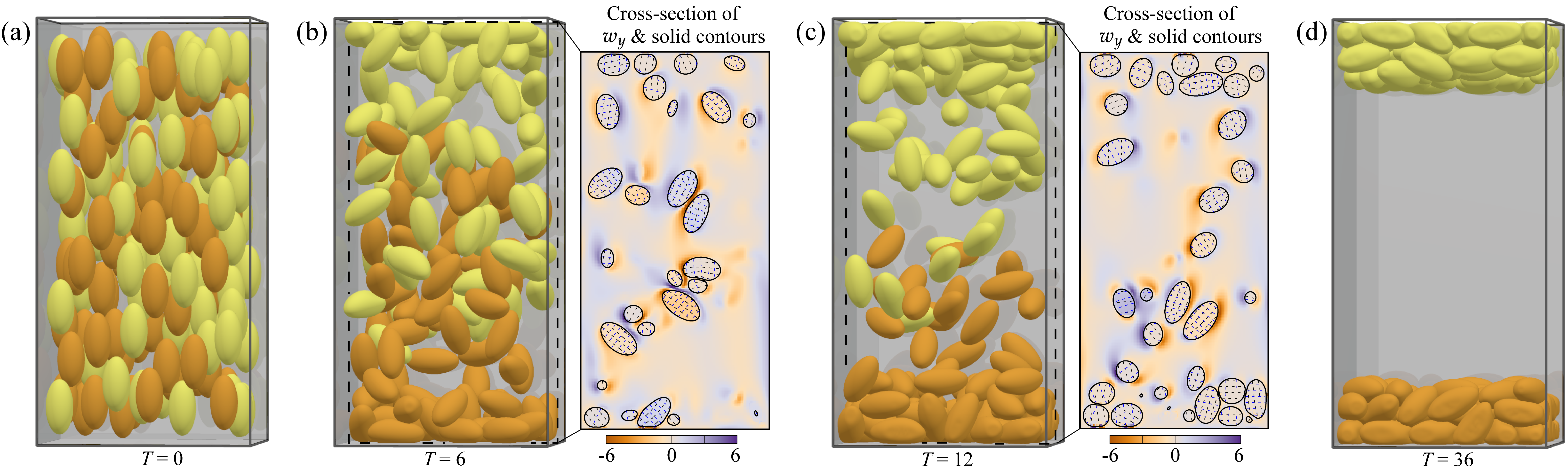
Figure 3: Various stages of 150 ellipsoids settling in a square cylinder (see SI for full movie). All ellipsoids have major axis $R=0.13$ initially aligned with $z$-direction, aspect ratio 2:1:1. Half of the ellipsoids are buoyant, $\rho_{s}/\rho_{f}=0.8$ (yellow) and the others are denser than the fluid $\rho_{s}/\rho_{f}=1.25$ (orange). Other parameters are $(L_{x},L_{y},L_{z},\rho_{f},G,\mu,\mu_{a},\gamma_{t},h,\epsilon)=(1,1,2,1,10^{-1},10^{-3},10^{-3},0,1/128,1/128)$. No-slip boundary conditions are applied on all the walls. In (b) and (c) cross-sections at $y=0.5$ are shown, color corresponds to the $y$ component of vorticity. Fluid–solid interfaces are plotted with a thick black line, and contours of reference map components $\xi_{x}$ and $\xi_{z}$ are plotted with black and blue dashed lines, respectively. A contact model among solid bodies via collision stress [26] is used. The maximum particle Reynolds number is approximately 20. This simulation was run with 48 MPI processes on Intel “Cascade Lake” and took 19 hours to simulate to $T=36$.

Table 1: Physical parameters (columns 2–3) used in the experiments by ten Cate et al. [40] and dimensionless simulation parameters (column 4–7). Experiment: sphere density $1120~{}\text{kg}/\text{m}^{3}$, diameter $15~{}\text{mm}$, and domain dimensions $10~{}\text{cm}\times 10~{}\text{cm}\times 16~{}\text{cm}$. Simulation: M, L, T are units of mass, length, and time, respectively. Length and time are rescaled by $l_{0}=0.1~{}\text{m}$ and $t_{0}=0.1~{}\text{s}$, respectively. Mass is rescaled in each case so that the fluid density is $1~{}\text{M/L}^{3}$. For all cases, $h=1/160,\epsilon=0.5h$.

	$\rho_{f}$	$\mu$	$\rho_{s}$	$\mu$	$\mu_{a}/\mu$	G
	($\text{kg/m}^{3}$)	(kg/(ms))	($\text{M/L}^{3}$)	($10^{-3}$M/(LT))	–	($\text{M/LT}^{2}$)
A	970	0.373	1.155	3.845	1	5.0
B	965	0.212	1.161	2.197	1	2.5
C	962	0.113	1.164	1.175	2	2.0
D	960	0.058	1.167	0.6042	4	2.0

Lid-driven cubic cavity with a sphere

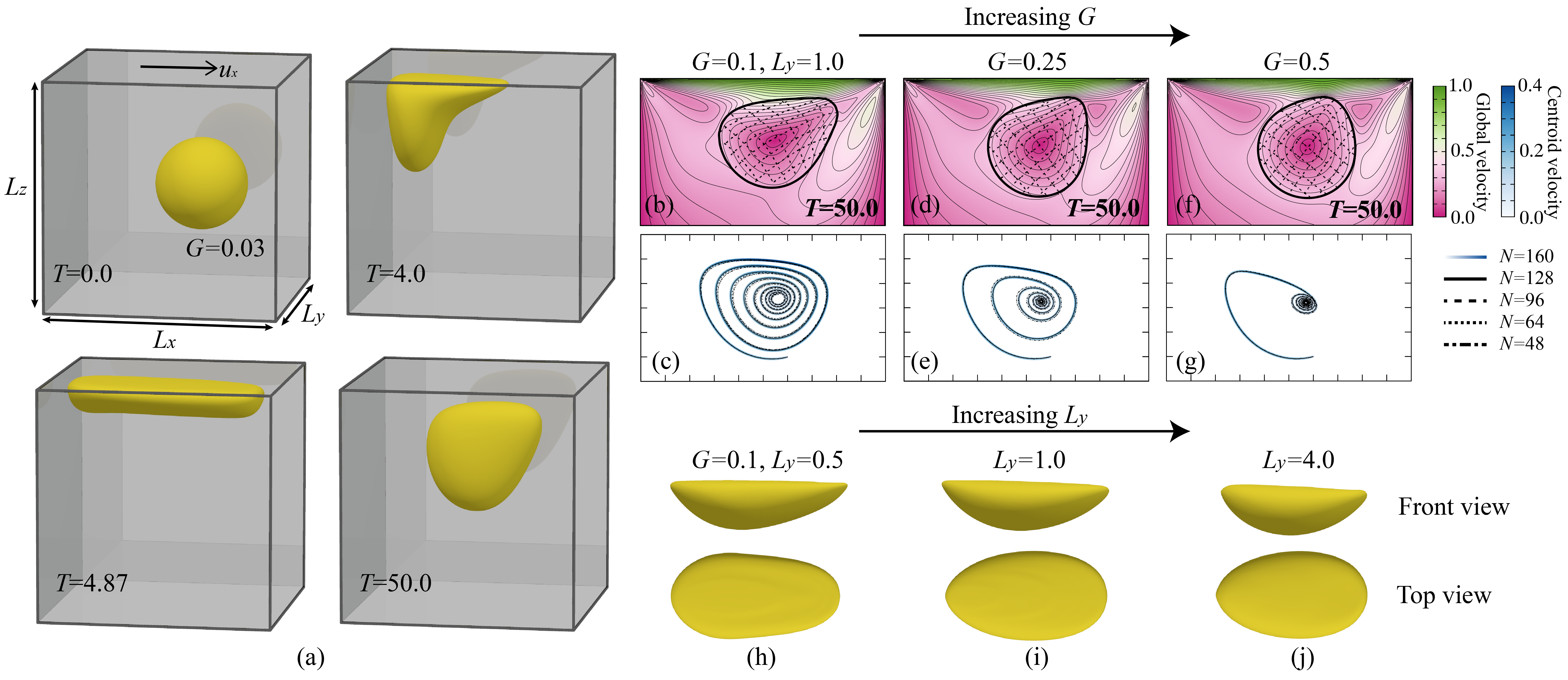
Figure 4: Simulations of a sphere in the lid-driven cavity. For all cases, parameters $(L_{x},L_{z},u_{x},\rho_{s},\rho_{f},\mu,\mu_{a},\epsilon)=(1,1,1,1,1,10^{-2},10^{-2},1.5h),\gamma_{t}\in[0,4],h\in[1/160,1/48]$. The sphere has radius $0.2$ and is initially centered at $(0.6,0.5L_{y},0.5)$. (a) 3D snapshots of a simulation at various times, $(L_{y},G)=(1,0.03)$. (b) Contours of the reference map and the interface are plotted against a background of velocity magnitude (heatmap and contours). A cross-section at $y=0.5$ and $T=50$ is shown, $(L_{y},G)=(1,0.1)$, $h=1/N$. (c) The trajectory of the sphere centroid from $T=0$ to $T=50$ of the sphere in (b). The color corresponds to the velocity magnitude of the centroid. (d), (f) The same as (b) but for solid shear moduli $G=0.25$ and $0.5$, respectively. (e), (g) The same as (c) but for solid shear moduli $G=0.25$ and $0.5$, respectively. (h), (i), (j) 3D shape of a deformed $G=0.1$ sphere at the closest approach to the top in cavity with $L_{y}=0.5,1.0,4.0$, respectively. See SI for additional parameters, movies, and trajectory data.

In computational fluid dynamics the lid-driven cavity has long been an important benchmark problem [49, 50]. Despite its simplicity, it exhibits rich flow dynamics due to varying cavity geometries, boundary conditions, and Reynolds numbers. In stark contrast to the extensive studies on the fluid problem in both 2D and 3D, results on lid-driven cavities with deformable boundaries and immersed solids are much fewer [20, 51, 52, 53]. In this section, we turn our attention to a neutrally buoyant deformable sphere in a lid-driven cavity, which to our best knowledge is the first 3D result of its kind.

Shown in Fig. 4(a), the cavity has size $L_{x}\times L_{y}\times L_{z}$ and two span aspect ratios, $L_{z}/L_{x}$ and $L_{y}/L_{x}$. The lid moves with velocity $\mathbf{u}_{\text{top}}=(u_{x},0,0)$ and no-slip boundary conditions are applied on all the other walls. We rescale length and velocity by $L_{x}$ and $u_{x}$, respectively. As a validation, we simulate lid-driven cavity flows without a solid, configured with various span aspect ratios and Reynolds numbers. Our results agree well with high accuracy benchmarks [49] (see SI for details).

A circular particle in a square lid-driven cavity in 2D has been investigated by Zhao et al. [51] and widely used as a validation case in later works [19, 54, 55, 56]. We simulate a sphere in a cubic cavity but choose parameters similar to those in the 2D test case to highlight qualitative differences in 3D (Fig. 4(b, c)). The middle cross-section of the deformed sphere (Fig. 4(b)) is qualitatively similar to the shape of the deformed circular particle at long time [56]. The distinctions between the two cases are more apparent in their centroid trajectories. Compared with the 2D case [19], although the centroid of a sphere in a cubic cavity (Fig. 4(c)) also converges to a stationary point, each spiral of its trajectory is much closer to the neighboring ones. There are several reasons for this, most notably the topological difference between an infinite cylinder and a sphere. Another reason is the reduced circulation due to lateral walls in the third dimension [50], which allows the sphere to interact with the moving lid for a longer time before being carried back to the center of the cavity by the flow.

We also simulate spheres with varying shear moduli. Snapshots of a simulation with $G=0.03$ are shown in Fig. 4(a). To our knowledge, this is the lowest shear modulus reported in the literature for cavity flow with deformable solids. In addition, as Fig. 4(e, g) show, as the shear modulus increases, the sphere exhibits distinct centroid trajectories. Fig. 4(d, f) offer some intuition for the qualitative changes. As a stiffer sphere moves toward and along the top lid, it deforms less and is able to separate earlier from driving flow. Consequently, a stiffer sphere is carried by the flow from the top right more toward the center than toward the bottom.

We also want to show the effect of the lateral walls on the solid deformation. We simulate a sphere with $G=0.1$ initially at $(0.6,0.5L_{y},0.5)$ in cavities with $L_{y}/L_{x}=0.5,4$. Fig. 4(h–j) show two views of the sphere at the closest approach to the top lid in each cavity. As the walls become farther apart, the sphere becomes less stretched lengthwise and less compressed vertically, again suggesting that a reduced circulation increases the strength of the interaction between the sphere and the moving boundary. We note that here we do not impose any repulsive forces on the sphere near the walls to avoid interfering with its dynamics, thus properly resolving the lubrication layer between the sphere and the boundaries is critical in keeping it from penetrating the walls. In simulations with a coarse resolution and a low $G$, a nonzero $\gamma_{t}$ is needed to dampen the motion of the interface near the boundaries.

In this section, we demonstrate that our numerical schemes, including the new extrapolation method, perform well under the stress of simulating extreme deformations near boundary singularities in a dynamic flow.

Swimming

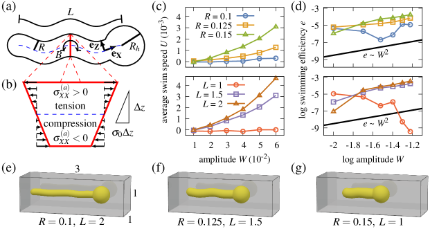
Figure 5: Swimming of flagellar objects driven by active bending moments. (a) Schematic of a swimmer. Swimmers have a spherical head of radius $R_{h}$ and a cylindrical body of length $L$ and a body radius $R<R_{h}$. The body is actuated by traveling wave of bending moments $B$ applied to vertical cross-sections (marked in red). (b) Expanded view showing the active in-plane stresses $\sigma^{(a)}_{XX}$ directed along the body’s long axis $\tilde{\mathbf{e}}_{X}$. The stress magnitude varies linearly with the height above the horizontal midplane (a dashed blue line). The swim speed $U$ (c) and efficiency $e$ (d) as a function of $W$, the bending wave amplitude, are presented for a variety of body shapes. Simulations in the top row vary $R$ with $L=1.5$, and those in the bottom row vary $L$ with $R=0.15$. (e–g) Body shapes, mid-stroke, are shown for several $R,L$ combinations. See SI for simulation movies. Steady-state measurements are taken at time $T$. $T=20$ for $R=0.15$, and $T=10$ otherwise. For all cases, $(L_{x},L_{y},L_{z},R_{h},\rho,G,\mu,\mu_{a},\gamma_{t},h,\epsilon)=(3,1,1,0.25,1,1,10^{-2},10^{-2},0,1/96,1/192)$.

We now apply the RMT to model swimming where the active deformations in the solid phase drive the motions in the system. Swimming has been an FSI problem of interest for decades [57, 58, 59]. To address the difficulty of resolving the full FSI, especially motions of the phase boundary, modelers often apply simplifications such as asymptotic analysis and scaling arguments. A related, widely applied numerical approach in the low Reynolds number regime is to abstract the swimmer into a one-dimensional collection of regularized singularities [6, 32, 60, 61, 62, 63]. As the swimmer undergoes prescribed deformation or active forcing, the resulting flow is a good approximation to the swimmer’s far field. However, this method is not well suited for contexts where the near field is of prime importance, such as dense suspensions of swimmers and swimming in tight confinement. These cases often require specializations [64, 65] or immersed boundary methods [8, 66]. Here, we show that the RMT naturally resolves the near field around finite-size swimmers in confined geometries. Despite being an Eulerian method, the RMT provides easy access to the reference map, allowing for straightforward definition of the active stresses in the swimmer’s body frame.

We begin with a description of our model swimmer, a cylindrical flagellum of length $L$ and radius $R$ with a spherical head of radius $R_{h}>R$ as shown in Fig. 5(a), and the active stress driving its cyclic deformation. We decompose the solid stress tensor into passive and active parts $\boldsymbol{\sigma}_{s}=\boldsymbol{\sigma}^{(\text{p})}+\boldsymbol{\sigma}^{(\text{a})}$, where $\boldsymbol{\sigma}^{(\text{p})}=\boldsymbol{\sigma}^{(\text{p})}(\mathbf{F})$ is the elastic stress tensor from previous sections. We seek to define a time-dependent active stress field $\boldsymbol{\sigma}^{(\text{a})}=\boldsymbol{\sigma}^{(\text{a})}(t,\boldsymbol{\xi},\mathbf{F})$ as a function of body position and local deformation, which will induce a planar bending wave traveling along the cylinder flagellum. First, we specify how body orientation is determined in the deformed frame. We assume without loss of generality that the reference frame coordinate system is centered on the flagellum and aligned with the swimmer. Denoting the reference frame’s orthonormal basis as $\{\tilde{\mathbf{e}}_{I}\}$, $I\in{X,Y,Z}$, we orient $\{\tilde{\mathbf{e}}_{I}\}$ so $\tilde{\mathbf{e}}_{X}$ points along the body toward the head and $\tilde{\mathbf{e}}_{Z}$ vertically up. The directions of these vectors in the deformed space, $\{\mathbf{e}_{I}\}$, where $\smash{\mathbf{e}_{I}=\mathbf{F}\cdot\tilde{\mathbf{e}}_{I}/\|\mathbf{F}\cdot\tilde{\mathbf{e}}_{I}\|}$, are also body-aligned as shown in Fig. 5(a).

Now, we define the active stress in terms of the reference map coordinates $\smash{X(\mathbf{x},t)=\tilde{\mathbf{e}}_{X}\cdot\boldsymbol{\xi}(\mathbf{x},t)}$ and $\smash{Z(\mathbf{x},t)=\tilde{\mathbf{e}}_{Z}\cdot\boldsymbol{\xi}(\mathbf{x},t)}$, which denote the reference distance along the cylinder and above the midplane, respectively. Bending moments are induced by axial stresses $\smash{\sigma_{XX}^{(a)}=\mathbf{e}_{X}\cdot\boldsymbol{\sigma}^{(a)}\cdot\mathbf{e}_{X}}$ of opposing sign about the midplane $Z=0$, as shown in Fig. 5(b), so we set $\sigma_{XX}^{(a)}=\sigma_{0}Z$ for simplicity. Letting the full tensor be traceless, we set

$$\boldsymbol{\sigma}^{(\text{a})}=\frac{3Z\sigma_{0}}{2}\left(\mathbf{e}_{X}\otimes\mathbf{e}_{X}-\frac{1}{3}\mathbf{1}\right),$$ (8)

where $\sigma_{0}\propto\cos(kX-\omega t)$ for some wavenumber $k$ and frequency $\omega$. Introducing the amplitude parameter $W=B/3GIk^{2}$, where $I$ is the cylinder’s cross-sectional area moment of inertia and $B$ a bending moment magnitude, we set

$$\sigma_{0}=3WGk^{2}\cos(kX-\omega t),$$ (9)

to systematically set bending moments across a range of $R$. We emphasize that $W$ is not a prescribed or measured vertical displacement, but a parameter derived from scaling arguments describing linear rod bending (see SI for details).

We nondimensionalize variables and parameters using length, time, and stress scales $l=2\pi/k$, $\tau=2\pi/\omega$, $\Sigma=G$. We simulate the dimensionless, uniform density system at constant $\rho,\mu$ and $R_{h}$ with varying $R$, $W$, and $L$. For each combination of parameters, we calculate the average swim speed $U$, shown in Fig. 5(c), and active power $\smash{P=\big{<}-\int_{\Omega_{s}}\boldsymbol{\sigma}^{(a)}:\nabla\mathbf{u}dV\big{>}}$, where $\left<*\right>$ denotes time averaging over many cycles of oscillation. We also calculate an approximate Lighthill efficiency $e=CU^{2}/P$ [67], shown in Fig. 5(d), where $C$ is a drag coefficient used to estimate the force required to tow the swimmer at velocity $U$. Mid-stroke body shapes for selected parameters are shown in Fig. 5(e–g). See SI for details and movies.

Broadly, swimming with the prescribed active stress is faster and more efficient at larger body sizes. This may be in part due to the changing Reynolds number $\textit{Re}_{s}$ corresponding to the time-averaged object motion, since it grows as $\textit{Re}_{s}\sim W^{2}$ over the range of simulated $W$ values; in contrast, the Reynolds number $\textit{Re}_{o}$ describing the swimming gait varies more slowly as $\textit{Re}_{o}\sim W$. Both $\textit{Re}_{s},\textit{Re}_{o}\in[10^{-4},0.1]$ for the results presented in Fig. 5 (see SI for details.) At large amplitudes, the efficiency scales as $e\sim W^{2}$, consistent with $U,P\sim W^{2}$. Notably, there is effectively no motion at $L=1$, suggesting a minimum length is required for efficient locomotion.

Conclusion and future work

The reference map technique is an efficient and flexible numerical method for FSI problems that involve many bodies, complex solid geometries, large deformations, and actuation. We have demonstrated the accuracy of its first 3D implementation, RMT3D, by convergence tests and comparisons against experimental data of settling spheres. We have also presented its applications to simulate settling of a large number of ellipsoids with varying density, a soft sphere in several lid-driven cavity flows, and swimmers with different body geometries, actuated by active stress.

A major future direction for the RMT is to address the issue of solid self-contact, which is a common occurrence in geometrically large deforming bodies, such as long slender structures and active swimmers. Other future work includes developing a more accurate contact model with physical boundaries to capture rebound behavior, as well as applying adaptive mesh refinement techniques to increase computational efficiency in many-body and multi-scale systems.

References

- [1] Mitul Luhar and Heidi Nepf. Flow-induced reconfiguration of buoyant and flexible aquatic vegetation. Limnology and Oceanography, 56:2003–2017, 11 2011.
- [2] Marek Bukowicki and Maria L. Ekiel-Jeżewska. Sedimenting pairs of elastic microfilaments. Soft Matter, 15(46):9405–9417, 2019.
- [3] Charles S Peskin. Flow patterns around heart valves: A numerical method. Journal of Computational Physics, 10(2):252–271, 1972.
- [4] Boyce E. Griffith, Xiaoyu Luo, David M. McQueen, and Charles S. Peskin. Simulating the fluid dynamics of natural and prosthetic heart valves using the immersed boundary method. International Journal of Applied Mechanics, 01(01):137–177, 2009.
- [5] Kelsey N. Lucas, Nathan Johnson, Wesley T. Beaulieu, Eric Cathcart, Gregory Tirrell, Sean P. Colin, Brad J. Gemmell, John O. Dabiri, and John H. Costello. Bending rules for animal propulsion. Nature Communications, 5(1), December 2014.
- [6] Yunyoung Park, Yongsam Kim, and Sookkyung Lim. Locomotion of a single-flagellated bacterium. Journal of Fluid Mechanics, 859:586–612, 2019.
- [7] Janna C. Nawroth, Hanliang Guo, Eric Koch, Elizabeth A. C. Heath-Heckman, John C. Hermanson, Edward G. Ruby, John O. Dabiri, Eva Kanso, and Margaret McFall-Ngai. Motile cilia create fluid-mechanical microhabitats for the active recruitment of the host microbiome. Proceedings of the National Academy of Sciences, 114(36):9510–9516, 2017.
- [8] Hanliang Guo, Lisa Fauci, Michael Shelley, and Eva Kanso. Bistability in the synchronization of actuated microfilaments. Journal of Fluid Mechanics, 836:304–323, 2018.
- [9] Charles S. Peskin. The immersed boundary method. Acta Numerica, 11:479–517, 2002.
- [10] Thomas G. Fai and Chris H. Rycroft. Lubricated immersed boundary method in two dimensions. J. Comput. Phys., 356:319–339, 2018.
- [11] Boyce E. Griffith and Neelesh A. Patankar. Immersed methods for fluid–structure interaction. Annual Review of Fluid Mechanics, 52(1):421–448, 2020.
- [12] Cyril W. Hirt, Anthony A. Amsden, and J. L. Cook. An arbitrary Lagrangian Eulerian computing method for all flow speeds. J. Comput. Phys., 14:227–253, 1974.
- [13] Sandra Rugonyi and Klaus-Jürgen Bathe. On finite element analysis of fluid flows fully coupled with structural interactions. Comput. Model. Eng. Sci., 2:195–212, 2001.
- [14] Clifford Truesdell. Hypo-elasticity. Indiana Univ. Math. J., 4:83–133, 1955.
- [15] H S Udaykumar, L Tran, D M Belk, and K J Vanden. An Eulerian method for computation of multimaterial impact with ENO shock-capturing and sharp interfaces. Journal of Computational Physics, 186(1):136–177, 2003.
- [16] Chris H. Rycroft and Frédéric Gibou. Simulations of a stretching bar using a plasticity model from the shear transformation zone theory. Journal of Computational Physics, 231(5):2155–2179, 2012.
- [17] Emmanuel Maitre, Thomas Milcent, Georges-Henri Cottet, Annie Raoult, and Yves Usson. Applications of level set methods in computational biophysics. Mathematical and Computer Modelling, 49(11–12):2161–2169, 2009. Trends in Application of Mathematics to Medicine.
- [18] Chun Liu and Noel J. Walkington. An Eulerian description of fluids containing visco-elastic particles. Archive for Rational Mechanics and Analysis, 159(3):229–252, 2001.
- [19] Kazuyasu Sugiyama, Satoshi Ii, Shintaro Takeuchi, Shu Takagi, and Yoichiro Matsumoto. A full Eulerian finite difference approach for solving fluid–structure coupling problems. J. Comput. Phys., 230(3):596–627, 2011.
- [20] Thomas Dunne. An Eulerian approach to fluid–structure interaction and goal-oriented mesh adaptation. Int. J. Numer. Methods Fluids, 51(9-10):1017–1039, 2006.
- [21] Thomas Richter. A fully Eulerian formulation for fluid–structure interaction problems. J. Comput. Phys., 233:227–240, 2013.
- [22] Thomas Wick. Fully Eulerian fluid–structure interaction for time-dependent problems. Comput. Method. Appl. M., 255:14–26, 2013.
- [23] Ken Kamrin. Stochastic and Deterministic Models for Dense Granular Flow. PhD thesis, MIT, 2008.
- [24] Ken Kamrin, Chris H. Rycroft, and Jean-Christophe Nave. Reference map technique for finite-strain elasticity and fluid–solid interaction. J. Mech. Phys. Solids, 60(11):1952–1969, 2012.
- [25] Boris Valkov, Chris H. Rycroft, and Ken Kamrin. Eulerian method for multiphase interactions of soft solid bodies in fluids. J. Appl. Mech., 82(4):041011, 04 2015.
- [26] Chris H Rycroft, Chen-Hung Wu, Yue Yu, and Ken Kamrin. Reference map technique for incompressible fluid–structure interaction. Journal of Fluid Mechanics, 898:A9, 2020.
- [27] Stanley Osher and James A. Sethian. Fronts propagating with curvature-dependent speed: Algorithms based on Hamilton–Jacobi formulations. J. Comput. Phys., 79(1):12–49, 1988.
- [28] James A. Sethian. Level Set Methods and Fast Marching Methods: Evolving interfaces in computational geometry, fluid mechanics, computer vision and materials science. Cambridge University Press, 1999.
- [29] Christopher W. MacMinn, Eric R. Dufresne, and John S. Wettlaufer. Fluid-driven deformation of a soft granular material. Phys. Rev. X, 5:011020, Feb 2015.
- [30] Eric D. Tytell, Chia-Yu Hsu, Thelma L. Williams, Avis H. Cohen, and Lisa J. Fauci. Interactions between internal forces, body stiffness, and fluid environment in a neuromechanical model of lamprey swimming. Proc. Natl. Acad. Sci., 107(46):19832–19837, 2010.
- [31] Becca Thomases and Robert D. Guy. Mechanisms of elastic enhancement and hindrance for finite-length undulatory swimmers in viscoelastic fluids. Phys. Rev. Lett., 113:098102, Aug 2014.
- [32] Cole Jeznach and Sarah D Olson. Dynamics of swimmers in fluids with resistance. Fluids (Basel), 5(1):14, 2020.
- [33] Morton E. Gurtin, Eliot Fried, and Lallit Anand. The Mechanics and Thermodynamics of Continua. Cambridge University Press, 2010.
- [34] Mark Sussman, Peter Smereka, and Stanley Osher. A level set approach for computing solutions to incompressible two-phase flow. J. Comput. Phys., 114(1):146–159, 1994.
- [35] Mark Sussman, Ann S Almgren, John B Bell, Phillip Colella, Louis H Howell, and Michael L Welcome. An adaptive level set approach for incompressible two-phase flows. Journal of Computational Physics, 148(1):81–124, 1999.
- [36] Jiun-Der Yu, Shinri Sakai, and James A. Sethian. A coupled level set projection method applied to ink jet simulation. Interfaces and Free Boundaries, 5(4):459–482, 2003.
- [37] Ann S. Almgren, John B. Bell, and William G. Szymczak. A numerical method for the incompressible Navier–Stokes equations based on an approximate projection. SIAM J. Sci. Comput., 17(2):358–369, 1996.
- [38] Phillip Colella. Multidimensional upwind methods for hyperbolic conservation laws. Journal of Computational Physics, 87(1):171–200, 1990.
- [39] Elbridge Gerry Puckett, Ann S. Almgren, John B. Bell, Daniel L. Marcus, and William J. Rider. A high-order projection method for tracking fluid interfaces in variable density incompressible flows. J. Comput. Phys., 130(2):269–282, 1997.
- [40] A. ten Cate, C. H. Nieuwstad, J. J. Derksen, and H. E. A. Van den Akker. Particle imaging velocimetry experiments and lattice-Boltzmann simulations on a single sphere settling under gravity. Physics of Fluids, 14(11):4012–4025, nov 2002.
- [41] A. Miyamura, S. Iwasaki, and T. Ishii. Experimental wall correction factors of single solid spheres in triangular and square cylinders, and parallel plates. International Journal of Multiphase Flow, 7(1):41–46, feb 1981.
- [42] Robert M. MacMeccan, J. R. Clausen, G. P. Neitzel, and C. K. Aidun. Simulating deformable particle suspensions using a coupled lattice-Boltzmann and finite-element method. Journal of Fluid Mechanics, 618:13–39, January 2009.
- [43] R.G.M. van der Sman. Drag force on spheres confined on the center line of rectangular microchannels. Journal of Colloid and Interface Science, 351(1):43–49, November 2010.
- [44] Sudeshna Ghosh and John M. Stockie. Numerical simulations of particle sedimentation using the immersed boundary method. Communications in Computational Physics, 18(2):380–416, August 2015.
- [45] Suresh Alapati, Woo Seong Che, and Yong Kweon Suh. Simulation of Sedimentation of a Sphere in a Viscous Fluid Using the Lattice Boltzmann Method Combined with the Smoothed Profile Method. Advances in Mechanical Engineering, 7(2):794198, February 2015.
- [46] P. Causin, J.F. Gerbeau, and F. Nobile. Added-mass effect in the design of partitioned algorithms for fluid–structure problems. Computer Methods in Applied Mechanics and Engineering, 194(42-44):4506–4527, October 2005.
- [47] Thomas G. Fai, Alejandra Leo-Macias, David L. Stokes, and Charles S. Peskin. Image-based model of the spectrin cytoskeleton for red blood cell simulation. PLOS Computational Biology, 13(10):1–25, 10 2017.
- [48] Anke Lindner. Flow of complex suspensions. Physics of Fluids, 26(10):101307, 2014.
- [49] S. Albensoeder and H.C. Kuhlmann. Accurate three-dimensional lid-driven cavity flow. Journal of Computational Physics, 206(2):536–558, July 2005.
- [50] Hendrik C. Kuhlmann and Francesco Romanò. The Lid-Driven Cavity. In Alexander Gelfgat, editor, Computational Modelling of Bifurcations and Instabilities in Fluid Dynamics, volume 50, pages 233–309. Springer International Publishing, Cham, 2019. Series Title: Computational Methods in Applied Sciences.
- [51] Hong Zhao, Jonathan B. Freund, and Robert D. Moser. A fixed-mesh method for incompressible flow–structure systems with finite solid deformations. Journal of Computational Physics, 227(6):3114–3140, March 2008.
- [52] Zhi-Qian Zhang, G. R. Liu, and Boo Cheong Khoo. A three dimensional immersed smoothed finite element method (3D IS-FEM) for fluid–structure interaction problems. Computational Mechanics, 51(2):129–150, February 2013.
- [53] Massimiliano M. Villone and Pier Luca Maffettone. Dynamics, rheology, and applications of elastic deformable particle suspensions: a review. Rheologica Acta, 58(3-4):109–130, April 2019.
- [54] H. Esmailzadeh and M. Passandideh-Fard. Numerical and Experimental Analysis of the Fluid-Structure Interaction in Presence of a Hyperelastic Body. Journal of Fluids Engineering, 136(11):111107, November 2014.
- [55] Iman Farahbakhsh, Hassan Ghassemi, and Fereidoun Sabetghadam. A vorticity based approach to handle the fluid–structure interaction problems. Fluid Dynamics Research, 48(1):015509, February 2016.
- [56] Hugo Casquero, Yongjie Jessica Zhang, Carles Bona-Casas, Lisandro Dalcin, and Hector Gomez. Non-body-fitted fluid–structure interaction: Divergence-conforming B-splines, fully-implicit dynamics, and variational formulation. Journal of Computational Physics, 374:625–653, December 2018.
- [57] Geoffrey Taylor. Analysis of the swimming of microscopic organisms. Proceedings of the Royal Society of London. Series A, Mathematical and physical sciences, 209(1099):447–461, 1951.
- [58] E. M Purcell. Life at low Reynolds number. American Journal of Physics, 45(1):3–11, 1977.
- [59] James Lighthill. Flagellar hydrodynamics. SIAM Review, 18(2):161–230, 1976.
- [60] Michael J Shelley and Tetsuji Ueda. The Stokesian hydrodynamics of flexing, stretching filaments. Physica D, 146(1):221–245, 2000.
- [61] Ricardo Cortez, Lisa Fauci, and Alexei Medovikov. The method of regularized Stokeslets in three dimensions: Analysis, validation, and application to helical swimming. Physics of Fluids, 17(3):031504–031504–14, 2005.
- [62] Karin Leiderman and Sarah D Olson. Swimming in a two-dimensional Brinkman fluid: Computational modeling and regularized solutions. Physics of Fluids, 28(2):21902, 2016.
- [63] Qiang Yang and Lisa Fauci. Dynamics of a macroscopic elastic fibre in a polymeric cellular flow. Journal of Fluid Mechanics, 817:388–405, 2017.
- [64] Hoang-Ngan Nguyen, Hoang-Ngan Nguyen, Sarah D Olson, Sarah D Olson, Karin Leiderman, and Karin Leiderman. Computation of a regularized Brinkmanlet near a plane wall. Journal of Engineering Mathematics, 114(1):19–41, 2019.
- [65] B. J. Walker, K. Ishimoto, H. Gadêlha, and E. A. Gaffney. Filament mechanics in a half-space via regularised Stokeslet segments. Journal of Fluid Mechanics, 879:808–833, 2019.
- [66] Arash Alizad Banaei, Marco Edoardo Rosti, and Luca Brandt. Numerical study of filament suspensions at finite inertia. Journal of Fluid Mechanics, 882, 2020.
- [67] M. J. Lighthill. Mathematical biofluiddynamics. Regional conference series in applied mathematics 17. Society for Industrial and Applied Mathematics, Philadelphia, 1975.