THU-Splines: Highly Localized Refinement on Smooth Unstructured Splines
Abstract
We present a novel method named truncated hierarchical unstructured splines (THU-splines) that supports both local -refinement and unstructured quadrilateral meshes. In a THU-spline construction, an unstructured quadrilateral mesh is taken as the input control mesh, where the degenerated-patch method ref:reif97 is adopted in irregular regions to define -continuous bicubic splines, whereas regular regions only involve B-splines. Irregular regions are then smoothly joined with regular regions through the truncation mechanism ref:wei18 , leading to a globally smooth spline construction. Subsequently, local refinement is performed following the truncated hierarchical B-spline construction ref:giannelli12 to achieve a flexible refinement without propagating to unanticipated regions. Challenges lie in refining transition regions where a mixed types of splines play a role. THU-spline basis functions are globally -continuous and are non-negative everywhere except near extraordinary vertices, where slight negativity is inevitable to retain refinability of the spline functions defined using the degenerated-patch method. Such functions also have a finite representation that can be easily integrated with existing finite element or isogeometric codes through Bézier extraction.
1 Introduction
Isogeometric analysis (IGA) was proposed to tightly integrate computer-aided design (CAD) with engineering simulation via employing the same spline-based basis in both sides ref:hughes05 ; ref:cottrell09 . Local refinement and extraordinary vertices111An extraordinary vertex is an interior vertex shared by other than four quadrilateral faces. (EVs) have been two of the most intensively studied topics in IGA to boost computational efficiency and support complex real-world geometries. Indeed, various methods have been proposed in each of the two topics. In the area of local refinement, T-splines ref:sederberg03 ; ref:sederberg04 ; ref:bazilevs10 and (truncated) hierarchical B-splines ref:forsey88 ; ref:kraft97 ; ref:vuong11 ; ref:giannelli12 are two of the mostly studied methods. On the other hand, in the area of supporting EVs, recent efforts have been devoted to recovering optimal approximation properties, such as geometrically continuous construction ref:kapl15 , manifold splines ref:majeed17 ; ref:bercovier17 , the degenerated patch (D-patch) method ref:reif97 ; ref:tnguyen16 ; ref:toshniwal17 , blended construction in 3D ref:wei18 and subdivision methods ref:xli19 ; ref:wei20 .
Moreover, several methods have also been proposed to support both local refinement and EVs at the same time, such as isogeometric spline forests ref:scott14 , truncated hierarchical Catmull-Clark subdivision ref:wei15a ; ref:wei15b , and analysis-suitable unstructured T-splines (ASUT-splines) with applications to Kirchhoff-Love shells ref:casquero20 . Particularly, ASUT-splines combine analysis-suitable T-splines ref:scott12 ; ref:veiga12 ; ref:li14 with the local D-patch construction ref:toshniwal17 , where the D-patch method is adopted to define -continuous splines around EVs while using regular -continuous B-splines away from EVs. While ASUT-splines show superior performance in Kirchhoff-Love shell problems ref:casquero20 , the need to resolve T-mesh constraints generally leads to refinement propagation beyond the region of interest. This becomes even more cumbersome when EVs are involved.
Therefore, we propose an alternative to ASUT-splines in this paper, namely truncated hierarchical unstructured splines (THU-splines), by combining truncated hierarchical B-splines (THB-splines) with the local D-patch construction. Unlike T-splines, hierarchical B-splines (HB-splines) have a definite termination condition to drive local refinement. Moreover, there is no need for HB-splines to resolve mesh constraints to guarantee desired properties for the underlying spline functions. These advantages make HB-splines be able to locally refine regions of interest flexibly without propagation. However, applying THB-like refinement to the local D-patch construction is challenging because various types of spline functions are defined in a local D-patch construction. These different splines need to be well organized such that all hierarchical splines defined on each element can be evaluated in a unified manner. Also due to this challenge, proving properties of the underlying hierarchical basis becomes technically much more involving. While we postpone most of the theoretical study in a forthcoming paper, we study how THU-splines retain an invariant geometric mapping in a constructive manner, in order to provide insights of how the truncation in THU-splines works. Moreover, we will use examples to show the numerical evidence of other claimed properties, such as refinability and partition of unity.
The paper is organized as follows. We first briefly review two closely related methods, that is, THB-splines in Section 2 and local D-patch construction in Section 3. In Section 4, we introduce our proposed method THU-splines. Section 5 presents several numerical examples to show flexibility, effectiveness and efficiency of THU-splines. In the end, we conclude the paper and comment on the future work in Section 6.
2 THB-splines
We briefly review THB-splines in this section. THB-splines ref:giannelli12 were proposed as an enhancement of hierarchical B-splines (HB-splines) ref:kraft97 to reduce support overlapping of B-splines from different hierarchical levels, which in turn leads to a sparse stiffness matrix with reduced band width. Moreover, THB-spline basis functions are piecewise polynomials that form a non-negative partition of unity.
In what follows, we explain the key steps of THB-spline construction in the unvariate setting, including initialization, selection, and truncation. While these key ideas are the same in other dimension cases, interested readers are referred to ref:giannelli12 ; ref:lyche18 for details.
2.1 Initialization
To start with, a set of univariate B-splines of degree (), defined on the knot vector , is given and initialized as the initial set of THB-spline basis functions, that is,
| (1) |
The initial domain serves as the entire domain of THB-splines, i.e., .
To facilitate explanation, we introduce a series of nested spaces spanned by the B-splines,
| (2) |
where is the predefined maximum level, and the set () is defined on the knot vector . Note that the degree is fixed at all levels. As will become clear shortly, only a small subset of is used and the full set is never generated in practice. is obtained by bisecting all the nonzero knot spans of , so knot vectors are nested as well,
| (3) |
A hierarchical construction involves a nested sequence of hierarchical domains,
| (4) |
This nested sequence implies a series of local refinements and it drives where to perform local refinement. For instance, once a set of THB-splines is initialized, we use to solve the problem of interest. According to a certain a posteriori error estimator, a subdomain of , which is in fact the domain at Level 1 (i.e., ), is marked to perform local refinement. Once is determined, THB-splines can be constructed accordingly.
THB-splines are constructed level by level, so we only need to study a generic two-level construction for selection and truncation: given the THB-splines that has been constructed up to Level () and (i.e., the subdomain of to be refined), we discuss how to build .
2.2 Selection
The selection mechanism, first proposed in ref:kraft97 and later generalized in ref:vuong11 , is aimed to ensure linear independence of resulting hierarchical basis functions. It is based on the relation between the support of a candidate B-spline and active subdomains of and . The selection at Level states that a B-spline is selected only if its support has a nonzero intersection with , the active subdomain at Level . All the selected Level- B-splines are collected in ,
| (5) |
where is the support of . On the other hand, at Level , a B-spline is selected only if its support is fully contained in . All the selected Level-() B-splines form the set ,
| (6) |
Selected B-splines are called active, and the complementary set of B-splines (i.e., and ) are passive. A prefix “H” will be added (i.e., H-active or H-passive) to emphasize the hierarchical refinement when the context is not evident; see Section 4. The subscript “0” in indicates the initial selection at Level with the entire being active. Certain functions in may latter become passive when Level is constructed from Level and the active Level-() subdomain changes from to . , , and are introduced to denote the index sets of , , and , respectively.
2.3 Truncation
The truncation mechanism, which enables reduced overlapping and partition of unity, plays the key role in THB-splines. We need the refinability relationship to explain the idea. Refinability states that a Level- B-spline can be expressed as a linear combination of certain Level-() B-splines,
| (7) |
where are coefficients obtained from the knot insertion algorithm ref:boehm80 , and () are called the children (or H-children, children in the hierarchical refinement) of . In fact, refinability is the reason for Eq. (2) to hold.
The truncation mechanism applies to when some of its children are active, and it discards the active children from Eq. (7). As a result, the truncated function of is defined as
| (8) |
which is also referred to as the inter-level truncation in this paper. Equivalently speaking, the coefficient in Eq. (7) is set to be by truncation if is active. Note that when all the children are passive (i.e., ), we have and thus . In other words, Eq. (8) can represent a generic definition including both truncated and non-truncated B-splines.
In summary, after selection of and , truncation is applied to certain B-splines in , leading to a set of truncated (active) B-splines at Level ,
| (9) |
The THB-spline basis functions up to Level are now obtained as
| (10) |
where note that when .
In Eq. (10), the local refinement is realized by enriching basis functions and it solely depends on . and are merely adjustments of existing basis functions to accommodate . Therefore, local refinement is effective only when ; otherwise we end up with . A non-empty implies that must be able to cover the support of at least one Level-() B-spline; see Eq. (6). This is indeed the only requirement for local refinement of THB-splines. It has a definite termination condition and it indicates a highly localized refinement with no propagation beyond the region of interest.
3 Local D-patch Construction
THB-splines are built upon B-splines that can only take structured meshes as input. However, our goal is to perform truncated hierarchical refinement on unstructured quad meshes that involve EVs. As refinability is the key requirement for building hierarchical splines, we choose the D-patch method that retains this property while producing -continuous splines in irregular regions, which we call D-patch splines in the following. D-patch splines have shown optimal convergence in solving the 2nd order PDEs (partial differential equations), near-optimal convergence in the 4th order problems ref:toshniwal17 , as well as superior performance in Kirchhoff-Love shells ref:casquero20 .
In contrast to the global D-patch construction ref:reif97 ; ref:tnguyen16 that leads to reduced continuity everywhere and proliferation of degrees of freedom, a local D-patch construction defines D-patch splines only in irregular regions while keeping B-splines elsewhere. Such a local construction has been explored with global refinement ref:toshniwal17 as well as local refinement via T-splines ref:casquero20 .
Here we review the local D-patch construction following ref:casquero20 , including Bézier extraction on unstructured meshes, D-patch construction around EVs, smooth transition to join D-patches with regular B-splines, and global refinement. Interested readers are referred to related literature ref:reif97 ; ref:toshniwal17 ; ref:casquero20 for further details.
3.1 Bézier extraction
We first introduce several terminologies of unstructured meshes with the reference to Fig. 1. An element is called an irregular element if any of its vertices222We use “vertex”, “edge” and “face” to emphasize mesh connectivity (or topology), whereas using “point” to carry the position or geometry information. “Element” and “face” are used interchangeably. is an EV; otherwise it is regular. An element is a boundary element if any of its vertices lies on the boundary; otherwise it is an interior element. The one-ring neighborhood of a vertex includes all the elements sharing this vertex; recursively, the -ring () neighborhood is the ()-ring neighborhood together with those sharing vertices with the ()-ring neighborhood. The neighborhood of an element can be defined similarly. We adopt the following assumptions regarding the input mesh to simplify discussion.
-
•
An irregular element can only have one EV;
-
•
A boundary vertex can only be shared by either one or two elements; and
-
•
An irregular element must not lie in the three-ring neighborhood of any boundary vertex.
Each vertex corresponds to a control point, and we call such points V-points (i.e., vertex points). Each edge is assigned with a non-negative real number called the knot span or knot interval, which is used to define element (parametric) domains as well as spline functions. For simplicity, we adopt a semi-uniform configuration of knot intervals where all edges have a unit knot interval except for those perpendicular to the boundary, which have a zero knot interval. As a result, edges around EVs all have the same knot intervals, which indeed is a necessary assumption for the D-patch construction ref:reif97 .
| (a) | (b) |
 |
|
| (c) | (d) |
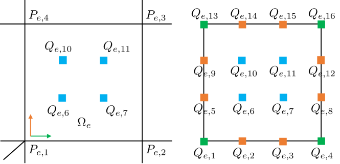
Note that given the third assumption regarding the input mesh, Bézier extraction is never needed for elements near the boundary. Without loss of generality, we next explain how to extract a Bézier representation for an irregular element ref:scott13 . Fig. 2(a) shows as a generic irregular element , where () are its 4 vertices, and is an EV. In the bicubic case, Bézier extraction is to find the Bézier control points () corresponding to . They can be divided into face, edge and vertex Bézier points, and they are called FB-points, EB-points, and VB-points, respectively; see Fig. 2(b). The 4 FB-points are computed as convex combinations of the 4 element corners, that is,
| (11) |
As shown in Fig. 2(c, d), EB- and VB-points are simply an average of their neighboring FB-points, for examples,
| (12) | ||||
where is the number of faces sharing , also called the valence of .
Now let denote the vector of Bézier points of , and and contain the V-points and FB-points of the one-ring neighborhood of , respectively. From Eqs. (11, 12), we observe that can be obtained through either
| (13) |
or
| (14) |
where the matrix contains the averaging coefficients in Eq. (12), and is the extraction matrix with coefficients from both Eqs. (11, 12). When , Eqs. (13, 14) indicate Bézier extraction for a regular bicubic B-spline element.
The Bézier representation of is written as
| (15) |
where is the vector of bicubic Bernstein polynomials. is expressed as,
| (16) |
where “” and “/” denote remainder and quotient operations, respectively; and
| (17) |
Alternatively, the surface patch can also be expressed in terms of and the associated spline functions ,
| (18) |
On the other hand, Eqs. (15, 18) must be equivalent, leading to
| (19) |
where we have used Eq. (14) to arrive at the last term. According to the arbitrariness of , we conclude that
| (20) |
Similarly, the surface patch can also be written with FB-points ,
| (21) |
The central idea of Bézier extraction is to express each spline function as a linear combination of Bernstein polynomials, which enables general spline functions to be easily integrated with existing finite element and isogeometric codes. While in regular elements, and are actually bicubic and B-splines, respectively, they are only -continuous in irregular elements. The D-patch construction essentially adjusts (or ) to yield smooth spline functions, which we discuss in the following.
3.2 D-patch method
In a local D-patch construction, the D-patch method is only adopted in regions around EVs, where we need to add necessary face-based control points and define their associated splines. Face-based control points are referred to as F-points in the following. Splines associated with V-points and F-points are referred to as V-splines and F-splines, respectively.
Enrichment via adding F-points. We introduce enriched elements to guide where to add F-points. Initially, all irregular elements are defined as enriched elements in the input mesh, whereas all the other elements are non-enriched elements. Enriched elements in refined meshes follow an “inheritance” rule, which will be discussed in Section 3.4.
Four F-points are then added to each enriched element. In fact, F-points are equivalent to FB-points, and they are obtained according to Eq. (11) in the input mesh. As a result, the control mesh of a local D-patch representation consists of both V-points and F-points; see Fig. 3. However, while all the F-points of enriched elements are active in the sense that they are used in the local D-patch representation, not all V-points are active. A V-point is passive if all its one-ring neighboring elements are enriched elements; otherwise it is active. A prefix “D” will be added to emphasize the context of local D-patch representation when necessary to distinguish those in hierarchical refinement. Clearly, all EVs are passive according to this definition. Essentially, passive V-points are replaced by their neighboring F-points. Note that such a control mesh corresponds to the analysis space discussed in ref:toshniwal17 .
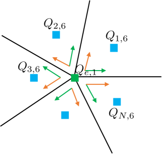
Definition of D-patch splines. We next briefly discuss the smooth D-patch splines around an EV that is shared by elements , . Interested readers are referred to ref:reif97 ; ref:toshniwal17 ; ref:casquero20 for details. D-patch splines are developed based on the version in Eq. (21). This essentially involves smoothing the underlying surface patches around the EV, so we first proceed from the perspective of Bézier control points. Starting from Eq. (13), we refine the Bézier patch via a split,
| (22) |
where () is the split matrix obtained from the well-known de Casteljau’s algorithm ref:boehm99 , and represents control points of the refined Bézier patch corresponding to the subelement ; see Fig. 4. In particular, .

In the D-patch method, a smooth representation is achieved by adjusting all , , , which are collected into a vector . This is done through a linear projection matrix ,
| (23) |
As a result, for every , , and the five points , , , and are coplanar; see indices in Fig. 4. The reminder of stays the same, and the resulting Bézier surface patches are smoothly joined together around the EV. The smoothing matrix corresponds to the idempotent version of the analysis space ref:casquero20 ; ref:toshniwal17 . Interested readers are referred there for further details. Note that although contains negative coefficients and thus leads to slightly negative spline functions, it guarantees refinability, which is the fundamental property required in a hierarchical spline construction.
Now we discuss the F-splines defined on an irregular element , which are associated with the F-points of the one-ring neighborhood of . They are piecewise-defined on the four subelements (, ) as
| (24) |
where the entries of come from with an proper arrangement for , and in particular, is an identity matrix. Comparing Eqs. (21, 24), we observe that by introducing matrices and , continuity is built into . Moreover, we have outside of the irregular element thanks to the split, or equivalently speaking, the presence of . Mostly importantly, it has also been proved that are refinable in the sense of Eq. (7); see ref:tnguyen16 . In the reminder of the paper, we omit “” over to keep notations simple.
3.3 Smooth transition
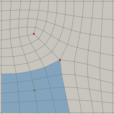
Next, we introduce how to smoothly join enriched and non-enriched elements in a local D-patch representation. The following terms are needed to facilitate the discussion. An interior edge is called an interface edge if it is shared by an enriched element and a non-enriched element. Vertices of interface edges are interface vertices. An element is then called a transition element if it contains an interface vertex. Note that transition elements can be regular or irregular; see Fig. 1. Now let and denote the index sets of V-points and F-points, respectively, and be the active subset of .
We now discuss the splines associated with the active V-points (), which include interface points () and the active regular points () that do not lie on the interface, that is, . Splines associated with are simply bicubic B-splines, whereas those associated with need truncation to enable a smooth transition between enriched and non-enriched elements. It is related but not the same as that introduced in the context of THB-splines. It was first proposed in blended B-splines ref:wei18 to recover the optimal convergence property when using unstructured hexahedral meshes. To distinguish, we refer to the truncation in a local D-patch representation as the same-level truncation. Recall that it is called the inter-level truncation in the context of THB-splines.
 |
|
| (a) | (b) |
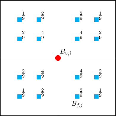
For the V-spline associated with an interface point (), we can express it in terms of its one-ring neighboring F-splines ,
| (25) |
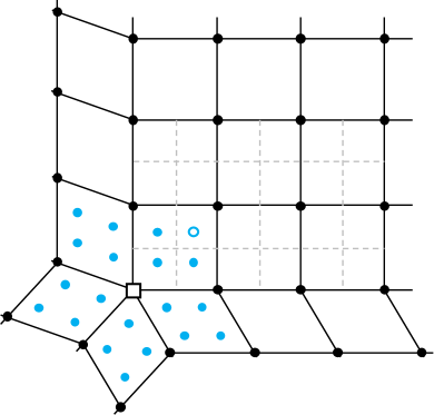
where the coefficients are obtained from Eq. (11) and they are illustrated in Fig. 5(a), is the index set of the F-points on the one-ring neighborhood of , and are the children (or D-children, children in the local D-patch representation) of . is defined by Eq. (24) if its F-point lies in an irregular element; otherwise it is defined by Eq. (21). Note that not all are associated with the F-points of enriched elements. As is an interface point, there must exist at least one non-enriched element in its one-ring neighborhood. F-points on non-enriched elements are not part of the control mesh in a local D-patch representation, and thus they are passive. In contrast, F-points of enriched elements are active.
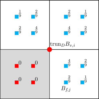
The same-level truncation for states that is set to be 0 if is active. In other words, active children of are discarded,
| (26) |
where is the index set of active F-points. As a result of truncation, is always a linear combination of regular B-splines. Fig. 5(b) shows an example of , where the red squares are active F-points as the gray element is enriched whereas the blue squares are passive and only serve as an auxiliary purpose to define . Therefore, the splines associated with interface points are truncated B-splines defined according to Eq. (26). From an element-wise perspective, truncation has no influence outside of transition elements in the sense that .
On the other hand, given an active non-interface point (), its associated spline is a B-spline and can be also expressed in the form of Eq. (26), where, however, truncation is trivial as , because we have by definition. In other words, holds for .
To this end, all spline functions of a local D-patch construction have been discussed, which form a partition of unity and are linearly independent ref:casquero20 . The local D-patch representation is written as
| (27) |
where we recall that , and and are (active) F-points and V-points, respectively. The corresponding matrix form is given as,
| (28) |
where and are vectors of V-splines and F-splines, respectively, and includes both regular B-splines () and truncated B-splines ().
3.4 Global refinement
Finally, we discuss how to perform global -refinement for a local D-patch representation. In the absence of EVs, -refinement of a B-spline patch is straightforward through the knot insertion algorithm, where the underlying geometric mapping stays the same during refinement. We call such a refinement the consistent refinement. However, consistent refinement is usually not available when EVs are involved. Currently, only two methods333We only focus on methods based on quadrilaterals. have this property: the D-patch method and subdivision. In fact, subdivision implies a large family of methods that feature an infinite piecewise definition of splines in irregular regions. Interested readers are referred to ref:xli19 ; ref:wei20 for some of the latest developments that aim to recover optimal convergence rates.
Consistent global refinement of a local D-patch representation consists of a topological step and a geometric step. The topological step deals with mesh connectivity as well as inheritance of enriched elements, whereas the geometric step computes control point coordinates of the refined mesh. Elementwise definitions of basis functions are discussed as well after the topological step.
Topological step. In the topological step, every element with a nonzero (parametric) measure is equally subdivided into 4 child elements. If a zero-measure element has a pair of opposite edges with nonzero knot intervals, it is subdivided into 2 child elements at the midpoints of such edges. Recall that irregular elements in the input mesh are marked as enriched elements. Subsequently in a refined mesh, elements in the ()-ring neighborhood of each EV are marked as enriched elements, where is number of global refinements. We observe the following: (1) regular elements in a refined mesh can be enriched elements; (2) child elements of a enriched element are always enriched elements; and (3) for a transition element that is not enriched, some of its child elements are also enriched, which are in fact the ()-ring neighborhood of an EV. Such an inheritance pattern of enriched elements ensures that the irregular region in the initial local D-patch representation is maintained throughout refinements, which is the key to guaranteeing refinability ref:toshniwal17 .
Elementwise definitions of basis functions. Once topological step is finished, basis functions of a refined mesh can be defined accordingly. Their definitions vary among different element types: regular elements that are not transition or enriched (type-R), non-transition enriched elements (type-E), and transition elements (type-T). A type-R element only involves 16 B-splines. -continuous splines are defined on a type-E element, which are D-patch splines if the element is irregular and 16 B-splines otherwise. On the other hand, a type-T element (no matter if the element is enriched or not) may involve a mix of all kinds of splines, such as V-splines (including B-splines and truncated B-splines) and F-splines (including B-splines and D-patch splines). As V-splines () can be expressed as linear combinations of F-splines (), we adopt the following matrix form to compactly organize all these splines on a transition element,
| (29) |
where coefficients of the matrix come from Eq. (26), is an identity matrix, and subscripts “” and “” again denote active and passive splines, respectively.
Geometric step. Positions of control points in a refined mesh are determined in the geometric step. Overall, all the coordinates are determined through the knot insertion algorithm. As has been discussed in ref:wei18 , this simple and unified computation is enabled by the (same-level) truncation.
The computation of point coordinates has two cases: B-spline refinement for non-enriched elements, and Bézier refinement for enriched elements. First, for a surface patch restricted to a non-enriched element (no matter if the element is transition or not), it is simply a B-spline patch when we only focus on its V-points. All the V-points of refined patches are obtained through the knot insertion algorithm applied to such a B-spline patch. Moreover, when the non-enriched element is a transition element, recall that some of its child elements are enriched elements, whose F-points are added according to Eq. (11).
Second, for a surface patch restricted to an enriched element, the corresponding local D-patch representation is first converted to its Bézier representation. Refinement is then applied to this Bézier patch using de Casteljau’s algorithm. In each of the resulting child Bézier patches, the 4 interior Bézier control points are added to the corresponding element (which must be an enriched element by definition) as the F-points.
To this end, both basis functions and control points are defined for a refined mesh. Its local D-patch representation has the same form as Eq. (28).
4 THU-Splines
We introduce the proposed method in this section, namely truncated hierarchical unstructured splines (THU-splines). Following the construction of THB-splines, we discuss the three steps in constructing THU-splines: initialization, selection, and truncation. Among them, truncation becomes particularly complex due to the presence of two kinds of truncation: the same-level truncation and the inter-level truncation.
4.1 Initialization
THU-splines are initialized with the local D-patch construction on an input unstructured quad mesh . For the ease of discussion, we introduce a series of consecutively refined meshes, , where is the predefined maximum number of refinements, and is a global refinement of () according to Section 3.4. Note that global refinement is never actually performed and these globally refined meshes are introduced only to simplify explanation. Correspondingly, a local D-patch basis , which only consists of D-active splines, is constructed on each . The initial THU-spline basis is given by . Moreover, with a closely related proof (Proposition 4.4, ref:toshniwal17 ), we conjecture that refinability holds for , for which we will show numerical evidence in Section 5.
Let and denote the index sets of F-points and active V-points of , respectively. Note that , where passive F-points () are introduced as an auxiliary means to define truncated B-splines associated with interface points, and splines associated with do not belong to .
4.2 Selection
The same as in Section 2, we focus on constructing from . Following Eq. (4), we assume that a series of nested hierarchical domains is given to guide local refinement. However, we need to define the “” operation in Eq. (4) for unstructured meshes. Let be a collection of all quad elements in . () is defined similarly but does not necessarily contain all elements of . means that every element in is a child element of a certain element in . In other words, is obtained by locally refining certain elements in ; after refinement, the parent elements of those in are no longer used and thus they are marked as passive. The active subdomain of consists of all active elements at Level .
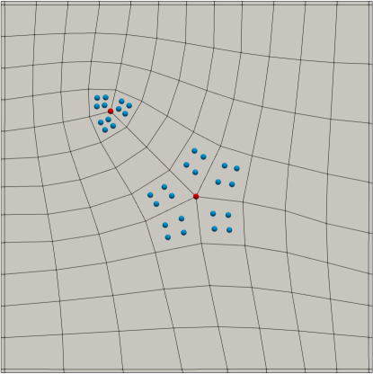
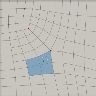
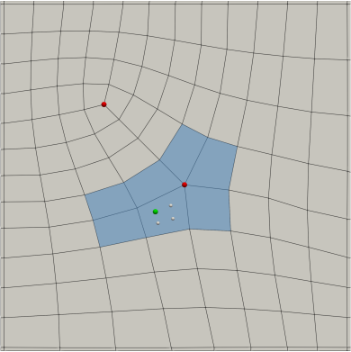
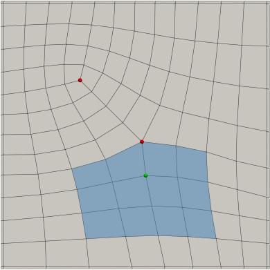
It is left to define the support of every basis function to apply the selection mechanism. Given a generic basis function (whose control point is denoted as ), its support, , is defined as a collection of certain elements in . There are four cases depending on the type of : (1) a V-point that is not on the interface, (2) an F-point on a regular element, (3) an F-point on an irregular element, and (4) an interface point; see Fig. 6.
 |
|
| (a) Case 1 | (b) Case 2 |
 |
|
| (c) Case 3 | (b) Case 4 |
In Case (1), is a bicubic B-spline, so is the two-ring neighborhood of . In Case (2), is a bicubic B-spline with doubly repeated knots, and is the one-ring neighborhood of . When is an F-point, its one-ring neighborhood means the one-ring neighborhood of its closest V-point. As a special case, the F-point in Fig. 2(b), although being on an irregular element, also falls into Case (2), whereas the other three (, and ) belong to Case (3).
Case (3) must involve a neighboring EV, and is defined as a D-patch spline. consists of two parts. First, the same as Case (2), has support on the one-ring neighborhood of . Moreover, is defined using the smoothing matrix such that it also has support on the one-ring neighborhood of the EV. The union of the two one-ring neighborhoods yields .
In Case (4), (more precisely, ) is a truncated B-spline that is expressed as a linear combination of certain D-passive B-splines. Therefore, its support is the union of all the one-ring neighborhoods of these D-passive F-points.
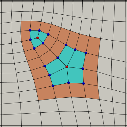
With the hierarchical domains and the support of splines well defined, the selection mechanism follows the same as those in Eqs. (5, 6) to collect all the H-active splines as and ; see an example in Fig. 7. Note that during selection, only D-active splines at each level can be selected to be H-active or H-passive, whereas D-passive ones only serve as an auxiliary purpose to help define truncated B-splines and they never enter the selection procedure. In other words, D-passive functions are neither H-active nor H-passive.
 |
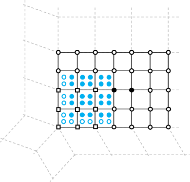
|
| (a) Level | (b) Level |
Finally, recall that needs to be large enough such that at least one Level-() spline function can be added to . In the THU-spline construction, this condition can be easily guaranteed if the parent elements of those in are a collection of one-ring neighborhoods of certain Level- points. In this manner, at least contains the two-ring neighborhood of a Level-() point. As the largest support in the above four cases is a two-ring neighborhood, a Level-() spline can always be added.
4.3 Truncation
The inter-level truncation follows the same as in Eq. (8). Certain H-active Level- functions are truncated. As a result, is changed to , and is constructed according to Eq. (10). Although the expressions stay the same as those in THB-splines, evaluation of THU-splines becomes much more involving because there are various types of splines rather than a single type as in THB-splines.
Without loss of generality, we study the THU-splines defined on a transition element , where we consider two levels (Levels and ) to simplify explanation. Following ref:bornermann13 , we evaluate all levels of H-active functions ( and ) with the functions (both H-active and H-passive) at the highest level, and we write it in the matrix form,
| (30) |
where the coefficients of come from Eq. (8), and spline functions in and () are from and , respectively. Note that the inter-level truncation has been incorporated for through the zero submatrix corresponding to .
We further split and as V-splines (, ) and F-splines (, ). As a result, Eq. (30) becomes
| (31) |
where because an F-spline can only have F-splines as its children. Moreover, can be evaluated according to Eq. (29), that is, , where is a vector of D-passive F-splines that do not belong to . Substituting this into Eq. (31), we have
| (32) |
where contains the full set of F-splines (including both D-active ones , and D-passive ones ) defined on the transition element at Level . Eq. (32) implies that THU-splines defined on a transition element can be evaluated in this unified manner as linear combinations of F-splines. The key is to obtain elementwise . With the two kinds of truncation, it can be shown that each column sum of equals to one. Therefore, THU-splines form a partition of unity. While we postpone the related proofs to a forthcoming paper, we will show numerical evidence in Section 5.
When is a non-transition enriched element (i.e., type-E), only F-splines are involved. In other words, we have in Eq. (31). In contrast, when is a type-R element, only B-splines are involved and they not truncated. Moreover, as no F-splines are involved. In fact, this latter case coincides with standard THB-splines.
4.4 Consistent refinement with THU-splines
We discuss how THU-splines can achieve a consistent refinement in this section. We approach it in a constructive manner to show how the two kinds of truncation work together to retain this property.
We assume that only two levels (i.e., and ) are involved to provide insights of construction while keeping notations simple. Globally refined meshes ( and ) and and their bases ( and ) are in place to help discussion. Also recall the following notations for index sets at Level :
-
•
and : D-active and D-passive F-points/splines, respectively;
-
•
: D-active V-points/splines; and
-
•
: H-active points/splines (which can be F- or V-points/splines).
In what follows, we start with Level alone and then add back Level . Without loss of generality, we study a transition element at Level , , which can be enriched or non-enriched. Its surface patch can be written as follows with a full set of Level-() F-splines,
| (33) |
which is essentially the same as Eq. (21). Next, we express in terms of D-active points/splines only. A D-passive F-point is obtained through its neighboring D-active V-points at the same level, so for , we have
| (34) |
which is in fact the same as Eq. (13), with . In fact, there are only four of that are nonzero. Substituting Eq. (34) to Eq. (33), we have
| (35) | ||||
where note that we have used the definition of the same level in the last equation; see Eq. (26). Eq. (35) is the local D-patch representation and it is indeed equivalent to Eq. (27).
Now we add to Eq. (35) the refinement relation between Levels and . A Level-() D-active V-point () is computed with the Level- D-active V-points,
| (36) |
where are the same coefficients as Eq. (7) and only a small number of them are nonzero. On the other hand, a Level-() D-active F-point is computed from Level- F-points (both D-active and D-passive), so for , we have
| (37) |
which is merely applying the B-spline knot insertion to doubly repeated knot vectors. When , is computed according to Eq. (34) (replacing with ).
We further divide and () into H-active and H-passive subsets, leading to , , , and . Next, starting from Eq. (35), we have
| (38) | ||||
We keep the terms corresponding to H-active subsets unchanged but further expand H-passive ones using Eqs. (36, 37),
| (39) | ||||
Notice that according to the selection mechanism of hierarchical splines, a Level- spline (F- or V-spline) is H-passive if and only if all its children are H-active; in other words, if any of its children is passive, then the spline is active. Therefore in the last equation in Eq. (39), we observe that when and , must be H-active, i.e., . Similarly, when , and , we have for ; when and , we must have for . Then after proper rearrangement, Eq. (39) becomes
| (40) | ||||
where we have used the definition of in the last term. Let and . We have
| (41) | ||||
with
| (42) |
and
| (43) |
Eq. (42) is merely a THB-spline that has a knot vector with doubly repeated knots, whereas Eq. (43) implies a mix of the same-level truncation and the inter-level truncation encoded in the coefficients and . Moreover, Eqs. (42, 43) correspond to and in Eq. (32), respectively. Although truncated splines in Eqs. (42, 43) have different forms, the key idea is essentially the same: A truncated spline is always expressed as a linear combination of certain passive splines.
Finally, with Eqs. (38, 41), the surface patch of the element can be written in terms of H-active splines only,
| (44) | ||||
which is also the general form of a THU-spline representation (with two levels). When is a Type-R (non-transition and non-enriched) element, only THB-splines are involved, i.e., , and . When is a Type-E (non-transition and enriched) element, only F-splines are involved, i.e., .
5 Numerical Examples
 |
|
| (a) | (b) |
 |
|
| (c) | (d) |
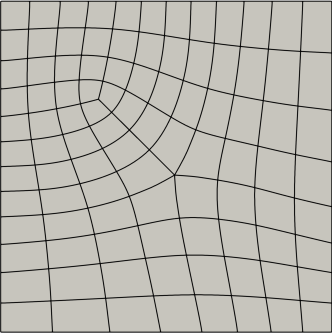
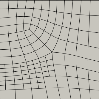
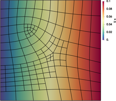
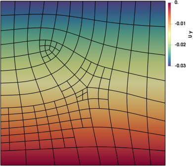
In this section, we present several examples to show its effectiveness and efficiency. We start with a patch test on a domain of unit square, where linear elasticity is solved using THU-splines. The unstructured quad mesh in Fig. 1 is taken as the input. Accordingly, an initial local D-patch representation is constructed, with its high-order spline mesh shown in Fig. 8(a). Next, we locally refine certain elements using THU-splines, which is intended to be general to include all types of elements: irregular, transition, and regular elements; see the resulting THU-spline mesh in Fig. 8(b). We use it to perform the patch test. Dirichlet boundary conditions , , and are imposed on the left, right, and lower boundaries, respectively, whereas free traction is applied to all the other boundaries. Isotropic and homogeneous material is assumed, where the Young’s modulus and the Poisson’s ratio are given as and , respectively. The displacement results are shown on the Bézier mesh in Fig. 8(c, d), where recall that each irregular element in Fig. 8(b) needs to be split into Bézier elements for the smooth D-patch construction. Moreover, we find that the -norm error of strains (, and ) is in the order of . In other words, the patch is passed with machine precision.
Successfully passing the patch test shows the applicability of THU-splines in engineering analysis. The numerical results also show supportive evidence regarding important properties of THU-splines. First, the involved THU-spline functions sum up to one and thus form a partition of unity. This confirms that the two kinds of truncation work as expected. Second, the involved THU-splines are linearly independent and thus constitute a basis. However, all these properties need to be rigorously studied, which is also the primary task of the future work.
 |
|
| (a) | (b) |
 |
|
| (c) | (d) |
Next, we use THU-splines to adaptively solve the biharmonic equation with the homogeneous Dirichlet and Neumann boundary conditions,
| (45) |
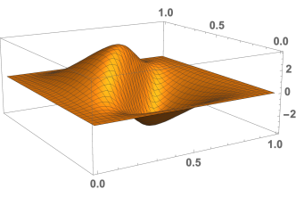
where is the outwards normal of . This is a 4th order PDE that requires continuity of the underlying basis functions. We again solve the problem on a unit square domain and start with the mesh given in Fig. 8(a). For the sake of convergence study, we use the following manufactured solution that has a large gradient across the line ,
| (46) |
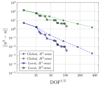
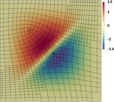
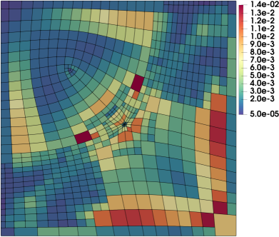
where and are two constants that control the behavior of the solution, and particularly, controls the “sharpness” of the gradient; see Fig. 9(a), where we use and . semi-norm error is used to drive local refinement to efficiently capture the gradient feature. Global refinement is taken as a reference. The convergence plot is summarized in Fig. 9(b) with respect to the square root of degrees of freedom (DOF). The approximate solution and the element-wise semi-norm error on the final locally refined mesh are shown in Fig. 9(c) and (d), respectively. We observe that compared to global refinement, THU-splines can achieve the same accuracy with much fewer DOF.
6 Conclusion and future work
In this paper, we have presented the construction method of THU-splines, a novel method that features a global smooth construction with the presence of EVs and supports flexible local refinement through the idea of THB-splines. Numerical evidence shows that THU-spline functions are refinable and form a partition of unity. Moreover, through solving the biharmonic equation with a manufactured solution, we show the efficiency of THU-splines compared to global refinement.
However, much remains to be studied to fully unleash the power of THU-splines. First of all, we will rigorously prove properties of THU-splines, including refinability, partition of unity, and linear independence. Once these foundations are ready, we will apply THU-splines to Kirchhoff-Love shell problems, where a posteriori error estimate is needed to automatically guide the adaptive analysis of THU-splines. The recent work reported in ref:coradello20 may well fit this purpose with the adaptation in irregular regions.
Acknowledgements.
X. Wei is partially supported by the ERC AdG project CHANGE n. 694515, as well as the Swiss National Science Foundation project HOGAEMS n.200021_188589.References
- [1] P. Antolin, A. Buffa, and L. Coradello. A hierarchical approach to the a posteriori error estimation of isogeometric Kirchhoff plates and Kirchhoff–Love shells. Computer Methods in Applied Mechanics and Engineering, 363:112919, 2020.
- [2] Y. Bazilevs, V. M. Calo, J. A. Cottrell, J. Evans, T. J. R. Hughes, S. Lipton, M. A. Scott, and T. W. Sederberg. Isogeometric analysis using T-splines. Computer Methods in Applied Mechanics and Engineering, 199:229–263, 2010.
- [3] M. Bercovier and T. Matskewich. Smooth Bézier surfaces over unstructured quadrilateral meshes. Springer International Publishing, 2017.
- [4] W. Boehm. Inserting new knots into B-spline curves. Computer-Aided Design, 12(4):199–201, 1980.
- [5] W. Boehm and A. Müller. On de Casteljau’s algorithm. Computer Aided Geometric Design, 16(7):587–605, 1999.
- [6] P. B. Bornermann and F. Cirak. A subdivision-based implementation of the hierarchical B-spline finite element method. Computer Methods in Applied Mechanics and Engineering, 253:584–598, 2013.
- [7] H. Casquero, X. Wei, D. Toshniwal, A. Li, T. J. R. Hughes, J. Kiendl, and Y. Zhang. Seamless integration of design and Kirchhoff–Love shell analysis using analysis-suitable unstructured T-splines. Computer Methods in Applied Mechanics and Engineering, 360:112765, 2020.
- [8] J. A. Cottrell, T. J. R. Hughes, and Y. Bazilevs. Isogemetric analysis: toward integration of CAD and FEA. John Wiley & Sons, 2009.
- [9] L. Beirão da Veiga, A. Buffa, D. Cho, and G. Sangalli. Analysis-suitable T-splines are dual-compatible. Computer Methods in Applied Mechanics and Engineering, 249–252:42–51, 2012.
- [10] D. R. Forsey and R. H. Bartels. Hierarchical B-spline refinement. Computer Graphics, 22:205–212, 1988.
- [11] C. Giannelli, B. Jüttler, and H. Speleers. THB-splines: the truncated basis for hierarchical splines. Computer Aided Geometric Design, 29:485–498, 2012.
- [12] T. J. R. Hughes, J. A. Cottrell, and Y. Bazilevs. Isogeometric analysis: CAD, finite elements, NURBS, exact geometry and mesh refinement. Computer Methods in Applied Mechanics and Engineering, 194:4135–4195, 2005.
- [13] M. Kapl, V. Vitrih, B. Jüttler, and K. Birner. Isogeometric analysis with geometrically continuous functions on two-patch geometries. Computers and Mathematics with Applications, 70(7):1518–1538, 2015.
- [14] R. Kraft. Adaptive and linearly independent multilevel B-splines. In A. L. Méhauté, C. Rabut, and L. L. Schumaker, editors, Surface Fitting and Multiresolution Methods, pages 209–218. Vanderbilt University Press, 1997.
- [15] X. Li and M. A. Scott. Analysis-suitable T-splines: characterization, refineability, and approximation. Mathematical Models and Methods in Applied Sciences, 24(06):1141–1164, 2014.
- [16] X. Li, X. Wei, and Y. Zhang. Hybrid non-uniform recursive subdivision with improved convergence rates. Computer Methods in Applied Mechanics and Engineering, 352:606–624, 2019.
- [17] T. Lyche, C. Manni, and H. Speleers. Foundations of spline theory: B-splines, spline approximation, and hierarchical refinement. Splines and PDEs: From Approximation Theory to Numerical Linear Algebra, Lecture Notes in Mathematics, 2219:1–76, 2018, Springer.
- [18] M. Majeed and F. Cirak. Isogeometric analysis using manifold-based smooth basis functions. Computer Methods in Applied Mechanics and Engineering, 316:547–567, 2017.
- [19] T. Nguyen and J. Peters. Refinable C1 spline elements for irregular quad layout. Computer Aided Geometric Design, 43:123–130, 2016.
- [20] U. Reif. A refineable space of smooth spline surfaces of arbitrary topological genus. Journal of Approximation Theory, 90(2):174–199, 1997.
- [21] M. A. Scott, X. Li, T. W. Sederberg, and T. J. R. Hughes. Local refinement of analysis-suitable T-splines. Computer Methods in Applied Mechanics and Engineering, 213-216:206–222, 2012.
- [22] M. A. Scott, R. N. Simpson, J. A. Evans, S. Lipton, S. P. A. Bordas, T. J. R. Hughes, and T. W. Sederberg. Isogeometric boundary element analysis using unstructured T-splines. Computer Methods in Applied Mechanics and Engineering, 254:197–221, 2013.
- [23] M. A. Scott, D. C. Thomas, and E. J. Evans. Isogeometric spline forests. Computer Methods in Applied Mechanics and Engineering, 269(0):222–264, 2014.
- [24] T. W. Sederberg, D. L. Cardon, G. T. Finnigan, N. S. North, J. Zheng, and T. Lyche. T-spline simplification and local refinement. ACM Transactions on Graphics, 23:276–283, 2004.
- [25] T. W. Sederberg, J. Zheng, A. Bakenov, and A. Nasri. T-splines and T-NURCCs. ACM Transactions on Graphics, 22:477–484, 2003.
- [26] D. Toshniwal, H. Speleers, and T. J. R. Hughes. Smooth cubic spline spaces on unstructured quadrilateral meshes with particular emphasis on extraordinary points: Geometric design and isogeometric analysis considerations. Computer Methods in Applied Mechanics and Engineering, 327:411–458, 2017.
- [27] A.-V. Vuong, C. Giannelli, B. Jüttler, and B. Simeon. A hierarchical approach to adaptive local refinement in isogeometric analysis. Computer Methods in Applied Mechanics and Engineering, 200:3554–3567, 2011.
- [28] X. Wei, X. Li, Y. Zhang, and T. J. R. Hughes. Tuned hybrid non-uniform subdivision surfaces with optimal convergence rates. 2020. arXiv:2003.12097.
- [29] X. Wei, Y. Zhang, T. J. R. Hughes, and M. A. Scott. Truncated hierarchical Catmull-Clark subdivision with local refinement. Computer Methods in Applied Mechanics and Engineering, 291:1–20, 2015.
- [30] X. Wei, Y. Zhang, T. J. R. Hughes, and M. A. Scott. Extended truncated hierarchical Catmull-Clark subdivision. Computer Methods in Applied Mechanics and Engineering, 299:316–336, 2016.
- [31] X. Wei, Y. Zhang, D. Toshniwal, H. Speleers, X. Li, C. Manni, J. A. Evans, and T. J. R. Hughes. Blended B-spline construction on unstructured quadrilateral and hexahedral meshes with optimal convergence rates in isogeometric analysis. Computer Methods in Applied Mechanics and Engineering, 341:609–639, 2018.