DCVNet: Dilated Cost Volume Networks for Fast Optical Flow

Abstract

The cost volume, capturing the similarity of possible correspondences across two input images, is a key ingredient in state-of-the-art optical flow approaches. When sampling for correspondences to build the cost volume, a large neighborhood radius is required to deal with large displacements, introducing a significant computational burden. To address this, a sequential strategy is usually adopted, where correspondence sampling in a local neighborhood with a small radius suffices. However, such sequential approaches, instantiated by either a pyramid structure over a deep neural network’s feature hierarchy or by a recurrent neural network, are slow due to the inherent need for sequential processing of cost volumes. In this paper, we propose dilated cost volumes to capture small and large displacements simultaneously, allowing optical flow estimation without the need for the sequential estimation strategy. To process the cost volume to get pixel-wise optical flow, existing approaches employ 2D or separable 4D convolutions, which we show either suffer from high GPU memory consumption, inferior accuracy, or large model size. Therefore, we propose using 3D convolutions for cost volume filtering to address these issues. By combining the dilated cost volumes and 3D convolutions, our proposed model DCVNet not only exhibits real-time inference (71 fps on a mid-end 1080ti GPU) but is also compact and obtains comparable accuracy to existing approaches.

1 Introduction

Optical flow, as a dense matching problem, is about estimating every single pixel’s displacement between two consecutive video frames, capturing the motion of brightness patterns. It is a classical and long-studied problem in computer vision, dating back to the early 1980s [9]. Optical flow has applications in a wide range of other problems, such as scene flow estimation [20], action recognition [25], and video editing and synthesis [1].

Figure 1: Comparison of inference speed, model size, and end-point-error (EPE) for different models. For each model, the circle radius indicates the number of parameters (larger radius means more parameters). The center of a circle corresponds to a model’s EPE. Our proposed DCVNet runs significantly faster than others, achieving real-time inference speed. At the same time, it is compact and obtains comparable error rate to existing approaches.

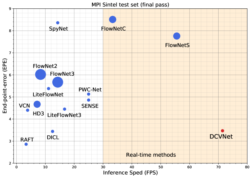
Like many other computer vision problems, state-of-the-art approaches for optical flow estimation are all based on deep neural networks. But unlike others, in the beginning, deep neural networks report inferior results compared to those of traditional well-engineered energy minimization approaches [6]. To reduce the performance gap, one approach is to stack multiple networks to increase the capacity [13], resulting in significant accuracy improvements. Simply increasing the capacity of the network, however, leads to huge networks and slower inference. Starting from [23], more and more classical principles derived from traditional optical flow estimation approaches are incorporated into neural network design, allowing deep neural networks to surpass traditional approaches in accuracy. In particular, the cost volume, which is a more discriminative representation for optical flow compared to concatenated feature representations of two images, is now an essential component for state-of-the-art approaches.

To build the cost volume, we need to sample pairs of locations between two input images in a neighborhood along both horizontal and vertical directions to compute their similarity (or cost). A big neighborhood is required to capture large displacements, but it leads to a very large cost volume and significant computational burden. Consequently, most existing models capture large displacements in a sequential manner by using cost volumes with small neighborhoods for computational efficiency purpose. Specifically, the coarse-to-fine strategy is widely adopted in state-of-the-art advances [27, 12, 32, 30], where a pyramid based on the feature hierarchy of deep Convolutional Neural Networks (CNNs) is built. In each pyramid level, the optical flow estimation in the previous level is used to construct the cost volume with the warping operation. Although a full-range cost volume is constructed in the recent ground-breaking work [28], a Recurrent Neural Network (RNN) is employed to process only a partial cost volume with a small neighborhood at each recurrence to capture large displacement sequentially.

For approaches using the sequential estimation strategy, optical flow in a particular pyramid level [27, 12, 32, 30] or recurrence stage [28] depends on the results from the previous one, resulting in lower inference speed. In this paper, we propose a novel approach for optical flow estimation, where cost volumes with different dilation rates are constructed to effectively capture both small and large displacements simultaneously, eliminating the sequential nature of the computation. As a result, our model is able to run at 71 frames per second (fps) for a Sintel-resolution image (with a size of $1024\times 436$) on a mid-end 1080ti GPU, achieving real-time inference. Optical flow estimation, as a fundamental task, is often integrated into other tasks. We believe fast optical flow computation is invaluable in order to avoid it being a bottleneck in the system design, leaving more room for other components.

In addition to being fast, an optical flow model should also be accurate and compact. This imposes challenges for the design of the decoder, which translates the cost volume to optical flow. Existing approaches usually employ 2D convolutions [27, 30] or separable 4D convolutions [32]. None of them, however, satisfies all of the requirements of accuracy, GPU memory consumption, and compactness at the same time. On the one hand, 2D convolutions flatten the cost volume and completely ignore the local spatial structure when sampling for displacement, leading to inferior accuracy and more network parameters [27, 12]. Recent work proposes displacement-invariant cost learning (DICL) to process a cost volume by applying 2D convolutions on each sampled displacement in the cost volume independently [30]. While this method has good accuracy, it consumes large amounts of memory. On the other hand, a separable 4D convolution consists of two successive 3D convolutions (and a non-linear layer in-between). When separable 4D convolution layers stack up, there are twice more layers than plain 3D ones, resulting in significantly more GPU memory consumption. To address these issues, we propose using 3D convolutions for cost volume filtering, which partially preserve the local structure of the cost volume and are thus more expressive than 2D ones with flattening. Compared with 2D convolutions with DICL [30] and separable 4D counterparts, the 3D version consumes much less memory. Consequently, our model is not only fast but also accurate and compact. Fig. 1 shows comparisons of our approach with others for end-point-error (EPE), inference speed, and model size.

To summarize, our contributions are three fold:

• We propose a novel approach for optical flow estimation, where cost volumes with different dilation rates are constructed to capture both small and large displacements, eliminating the need for sequential construction and processing of cost volumes.

• To address the limitations of current approaches for cost volume filtering, we propose using 3D convolutions, instead of the 2D and separable 4D variants. Our solution strikes a balance between accuracy, GPU memory consumption, and model size.

• By combining the dilated cost volumes and 3D convolutions for cost volume filtering, our proposed approach not only runs significantly faster (71fps on a mid-end 1080ti GPU), but is also compact and obtains comparable accuracy to existing approaches for optical flow estimation, reaching a new point on the speed-accuracy frontier.

2 Related Work

In this section, we discuss previous optical flow methods. Due to space limits, we focus on neural network-based approaches.

FlowNet, proposed in [6], has two variants, FlowNetS and FlowNetC, both of which have an encoder-decoder structure. FlowNetS simply concatenates the feature representations of the two images obtained from the encoder and lets the decoder learn how to compute optical flow. In contrast, FlowNetC constructs a cost volume by computing matching costs (or similarity) between two feature maps. To improve the accuracy, especially for large displacements, FlowNet2 [13] concatenates the FlowNetS and FlowNetC variants in a cascade, where the optical flow estimation is progressively refined. This is the first instance where a neural network reports better or on-par optical flow results with classical engineered approaches.

Although FlowNet2 achieves good accuracy, it has 162M parameters. The more compact SpyNet is proposed in [23]. It computes flow in a coarse-to-fine manner by using a pyramid structure borrowed from classical approaches. PWC-Net [27] extends the pyramid structure used in SpyNet. In each pyramid level, a cost volume is built by warping the second image’s feature map using the optical flow estimation in the previous level. As a result, large displacements can be captured in a sequential manner. A similar coarse-to-fine strategy is used in other approaches. LiteFlowNet [12] also uses a pyramid structure to estimate optical flow in a cascade manner and proposes a flow regularization layer. In the recent extension LiteFlowNet3 [11], an adaptive modulation prior is added to the cost volume, and local flow consistency is used to improve the final accuracy. HD³ [33] converts optical flow estimation into discrete distribution decomposition. SENSE [15] extends PWC-Net to solve optical flow and stereo disparity at the same time with a shared encoder. Instead of using a feature hierarchy for coarse-to-fine estimation, a Recurrent Neural Network is used in RAFT [28]. It builds a full-range cost volume capturing the similarity between all pairs of locations between two images. But at each recurrence step, only a partial cost volume in a small neighborhood is used to estimate an offset. This offset is used to move the estimated optical flow (displacement) iteratively closer to the optimum.

Such sequential estimation approaches are inherently slow as optical flow estimation at each pyramid level or recurrence step is dependent on the results in the previous one. In contrast, we build cost volumes with different dilation factors to effectively capture small and large displacements simultaneously. Consequently, our approach does not need the sequential estimation strategy, leading to a fast optical flow model during inference.

To translate a cost volume to optical flow estimation, existing approaches mainly rely on two types of models. For each location in the first image, a cost volume captures the similarity of all possible correspondences in both horizontal and vertical directions. It is therefore natural to apply 4D convolutions to process a cost volume. Due to lack of support in current libraries, however, 4D convolutions are not efficient. Instead, a separable 4D convolution is proposed in [32], which is converted into two successive 3D convolutions. Another widely used variant is to flatten a cost volume along the neighborhood width and height directions [27, 12] so that 2D convolutions can be used. In recent work [30], 2D convolutions are independently applied to each sampled displacement in the cost volume for displacement-invariant cost learning (DICL).

But none of these approaches are suitable to build an accurate and compact optical flow model with low GPU memory consumption. First of all, in analogy to the problems of flattening convolutional feature maps into feature vectors, 2D convolutions with flattening need more parameters in the network and ignore spatial structure in the cost volume. Instead, our approach partially preserves the structure of the cost volume, leading to better accuracy. Second, compared to our 3D convolution model, 2D convolutions with DICL [30] consume more GPU memory, as they need to process each sampled displacement independently. Finally, separable 4D convolutions have twice more layers than 3D plain ones and thus need much more GPU memory as well.

There are other approaches, whose efforts are complementary to ours. A set of improvements about model training protocols, including the data sampling process, model regularization, and data augmentation, are presented in ScopeFlow [2]. A learnable cost volume is proposed in [31], which considers the effectiveness of different feature channels by assigning different weights to different channels.

Using dilations in cost volumes is not completely new. FlowNetC [6] only uses a single dilation factor of 2, which does not fully exploit the potential of using dilations to capture large displacements. In Devon [18], dilated cost volumes are used as a replacement for the warping modules in a sequential coarse-to-fine estimation model. By sharp contrast to FlowNetC [6], we use multiple dilation factors to better capture small and large displacements. Additionally, unlike Devon [18], we use dilated cost volumes as an alternative for the sequential estimation strategy to compute optical flow. Moreover, our model achieves significantly better accuracy than both FlowNetC [6] and Devon [18].

Dilations are also used in a closely related task, stereo disparity estimation by StereoDRNet [4]. Although it is beyond the scope of optical flow estimation, we clarify the distinctions of our approach from it. In StereoDRNet [4], dilations are used in convolution layers, not the construction of the cost volumes, to process the cost volume, which we also use in our model (the ASPP module [5]).

3 Dilated Cost Volume Networks

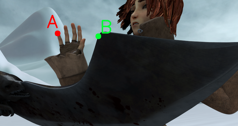
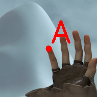
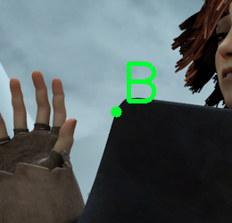
(a) input images	(b) dilation=1	(c) dilation=3

Figure 2: Illustration of using dilation to capture both small and large displacements. (a) input two images where points $A$ and $B$ move to $A^{\prime}$ and $B^{\prime}$, respectively. (b) two patches around $A$ in two images. (c) two patches around $B$ in two images. Blue dots in (b) and (c) correspond to candidate displacements when constructing cost volumes. With a small search radius (2 in this example), correct displacements (denoted by red and blue crosses, respectively) can be captured using two different dilation factors. Best viewed in color.

3.1 Dilated Cost Volumes

Given two input images $I_{1}$ and $I_{2}$ with height $H$ and width $W$, we extract their $L_{2}$-normed feature representations $\mathbf{x}_{1}^{s}$ and $\mathbf{x}_{2}^{s}$ at stride $s$ using a CNN, where $s$ corresponds to the spatial resolution downsample factor w.r.t. the input images. To search for the correct correspondence for a position $p=(x,y)$ in $\mathbf{x}_{1}^{s}$, we need to compare its feature vector with that of a candidate position $q=(x+u,y+v)$ in $\mathbf{x}_{2}^{s}$, where $u$ and $v$ are the offsets of the pixel from $p$ to $q$. To measure the similarity between feature vectors at $p$ and $q$, we have

$$\mathbf{c}^{s}(u,v,x,y)=f\left(\mathbf{x}_{1}^{s}(x,y),\mathbf{x}_{2}^{s}(x+u,y+v)\right),$$ (1)

where $f(\cdot,\cdot)$ is a function measuring the similarity between two feature vectors. Here we divide each of the vectors $\mathbf{x}_{1}^{s}$ and $\mathbf{x}_{2}^{s}$ into $C$ sub-vectors and compute the cosine similarity between each pair of corresponding sub-vectors. The output of $f$ therefore has $C$ dimensions. As we need to sample in a local 2D neighborhood for all possible correspondences, we have $u\in[-k,k]$ and $v\in[-k,k]$, where $k$ is the neighborhood radius. The cost volume size is thus $C\times U\times V\times\frac{H}{s}\times\frac{W}{s}$, where $U=V=2k+1$.

Due to the striding factor, such a cost volume $\mathbf{c}^{s}$ captures candidate horizontal displacements across two input images in the range of $s\odot[-k,k]$, where $\odot$ denotes the elementwise multiplication between a scalar and a vector. For simplicity, we use only the horizontal displacement for illustration here (vertical displacement can be analyzed similarly). To account for large displacements, which is critical for accurate optical flow estimation, either a larger stride $s$ or neighborhood radius $k$ can be used. Both of them are problematic, however. A larger stride means more downsampling and loss of spatial resolution. A large neighborhood radius, on the other hand, results in a large cost volume and heavy computation.

Instead, we propose to use dilation factors to construct cost volumes to deal with small and large displacement at the same time. Specifically, we have

$$\mathbf{c}^{s,d} (u^{d},v^{d},x,y)=f\left(\mathbf{x}_{1}^{s}(x,y),\mathbf{x}_{2}^{s}(x+u^{d},y+v^{d})\right),$$

$$\text{where}~{}u^{d}\in d\odot[-k,k],v^{d}\in d\odot[-k,k].$$ (2)

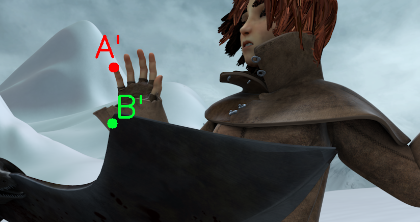
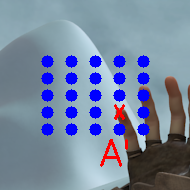
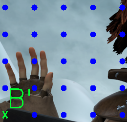
Here $d$ is a dilation factor. Now the search range of displacement over two input images is $sd\odot[-k,k]$. In this way, we can capture large displacements by having a large $d$ while maintaining small $k$ and $s$, which preserves both computational efficiency and spatial resolution for the cost volume. Fig. 2 illustrates how dilation helps capture both small and large displacements with a small neighborhood radius. Specifically, in this paper, we consider $s=8$ and $d\in\{1,3,5,9,13,21\}$. As we can see in Table 1, a displacement as large as 672 pixels can be captured using a dilation factor $d=21$, stride $d=8$, and neighborhood radius $k=4$.

As the dilation factors increase, the gap between candidate displacements also gets larger. To deal with this issue, we also build a cost volume with $s=2$ and $d=1$ to capture small and fine displacement. We do spatial sampling of 4 to make the spatial resolution compatible with the cost volumes constructed over the stride of 8. Finally, we concatenate all cost volumes over different strides and dilation factors. Our final cost volume has a dimension of $C^{\prime}\times U\times V\times\frac{H}{8}\times\frac{W}{8}$, where $C^{\prime}=D\times C$ and $D$ is the total number of dilation factors ($D=7$ in our case).

Table 1: Displacements over input images captured using different strides and dilation factors.

stride	dilation	candidate horizontal displacements
($s$)	($d$)
2	1	{-8, -6, -4, -2, 0, 2, 4, 6, 8}
8	1	{-32, -24, -16, 8, 0, 8, 16, 24, 32}
8	9	{-288, -216, -144, -72, 0, 72, 144, 216, 288}
8	21	{-672, -504, -336, -168, 0, 168, 336, 504, 672}

		optical flow hypotheses and fusion weights
(a) input	(b) optical flow and magnitude	(c) $s=2,d=1$	(d) $s=8,d=1$	(e) $s=8,d=13$	(f) $s=8,d=21$

Figure 3: Illustration of optical flow hypothesis fusion over different strides $s$ and dilation rates $d$. (a) Input images. (b) estimated optical flow (top) and flow magnitude (bottom). For (c)(d)(e)(f), top images are optical flow hypotheses and bottom images are pixel-wise fusion weights of the hypotheses. These hypotheses are normalized by the magnitude of the ground-truth optical flow for visualization purpose. For the optical flow magnitude and fusion weights, blue means a small value and red indicates a large one. In this example, optical flow of the static background and the person mainly come from the hypothesis with $s=8$ and $d=1$, while the hypotheses from different strides and dilation factors all contribute to the knife’s optical flow. Best viewed in color.

Figure 4: Pipeline of DCVNet. Feature representations of two input images are obtained from the encoder, which are used to construct the dilated cost volumes at different strides and dilation rates. A 3D U-Net is employed to process the cost volumes to produce a set of optical flow hypotheses. Finally, a 2D CNN is used to fuse those hypotheses and upsample it to the same spatial resolution of the input.

3.2 3D Cost Volume Filtering for Optical Flow

So far, we have introduced our dilated cost volumes. How can we translate such cost volumes into exact pixel-wise displacements, i.e., optical flow? Instead of directly regressing optical flow values, we do interpolation between all possible displacements similar to [32, 30]. Specifically, we have

$$\mathbf{f}^{s,d}=\sum_{i}^{UV}\omega_{i}^{s,d}\mathbf{f}_{i}^{s,d},$$ (3)

where $\sum_{i}^{UV}\omega_{i}=1$ and $\mathbf{f}^{s,d}$ is an optical flow vector hypothesis at stride $s$ with dilation $d$. We omit the pixel index for simplicity here. $\mathbf{f}_{i}^{s,d}=\left(\mu_{i}^{s,d},\nu_{i}^{s,d}\right)$ is a single 2D displacement, where $\mu_{i}^{s,d}\in sd\odot[-k,k],\nu_{i}^{s,d}\in sd\odot[-k,k]$. There are $UV$ such sampled displacements in a cost volume in total. To obtain the interpolation weights, we use a CNN taking our dilated cost volumes as input to estimate $\omega_{i}^{s,d}$.

Recall our dilated cost volumes have the shape of $C^{\prime}\times U\times V\times H^{\prime}\times W^{\prime}$ (here $H^{\prime}=\frac{H}{8},W^{\prime}=\frac{W}{8}$). 4D convolutions are needed to process such cost volumes, which lack native support in existing libraries. To this end, in VCN [32], separable 4D convolutions are proposed, consisting of two successive 3D convolutions (with intermediate non-linear layers). Another widely used option is to flatten the cost volumes to be of $C^{\prime\prime}\times H^{\prime}\times W^{\prime}$, where $C^{\prime\prime}=C^{\prime}\times U\times V$, squeezing the first three dimensions into a single one, so that 2D convolutions can be applied [27, 12]. DICL [30] avoids flattening the cost volume. Instead, it applies 2D convolutions over a cost volume with a shape of $C^{\prime}\times H^{\prime}\times W^{\prime}$ on $UV$ sampled displacements independently.

As we shall see in the experiment section, however, neither of these variants satisfies all the requirements of having an accurate and compact optical flow model without consuming too much GPU memory. On the one hand, 4D convolutions use two successive 3D convolutions, resulting in significantly more GPU memory consumption. On the other hand, 2D convolutions with flattening completely ignore the spatial structure of the cost volume, leading to inferior accuracy and substantially more parameters. 2D convolutions with DICL [30] need more GPU memory as well to process $UV$ displacements in the cost volume independently.

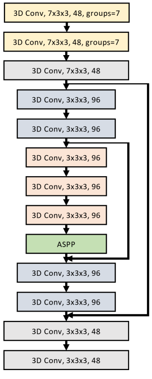
Our solution is to reshape the cost volume to be $C^{\prime}\times D^{\prime}\times H^{\prime}\times W^{\prime}$, where $D^{\prime}=U\times V$. It partially preserves the spatial structure of the cost volume. We then apply 3D convolutions to process the cost volume. As we will show in the experiment section, it strikes a balance between accuracy, model size, and GPU memory consumption. In particular, we use a U-Net [24], consisting of an encoder and decoder and skip connections between them. We add the ASPP (Atrous Spatial Pyramid Pooling) module [5] in the bottleneck of the U-Net model. A softmax is performed on top of the U-Net’s output to ensure that the constraints on $\omega_{i}^{s,d}$ are satisfied.

Given optical flow hypotheses across different strides and dilation factors according to Eq.(3.2), we obtain the final optical flow by weighted average over all hypotheses. Specifically, we have

$$\mathbf{f}=\sum_{s,d}\alpha^{s,d}\mathbf{f}^{s,d},$$ (4)

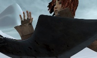
where $\sum_{s,d}\alpha^{s,d}=1$. Fig. 3 shows the examples of fusion of different optical flow hypotheses. We use another network with a set of 2D convolutions to estimate $\alpha^{s,d}$, which takes $\mathbf{f}^{s,d}$ and entropy of $\omega_{i}^{s,d}$ as input. Similarly, a softmax is performed on top of its output.

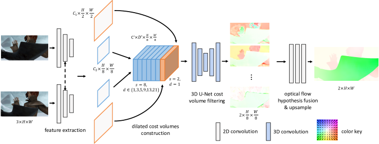
The architecture of our proposed dilated cost volume network (DCVNet) is illustrated in Fig. 4. We use the same feature encoder as used in [28] with Instance Normalization [29] layers to extract features of input images to construct the cost volume. We empirically found that having another context encoder is not helpful and yet significantly increases the number of parameters. There are no normalization layers for the rest of the DCVNet. We use Leaky ReLUs with a slope of 0.1 for the entire network. We use the same convex upsampling strategy used in [28] to upsample estimated optical flow to the input’s resolution. We provide more details of the network architecture in the supplementary material.

4 Experiments

4.1 Implementation Details

Pre-training. We train our model on the synthetic SceneFlow dataset [19] following [15], which consists of FlyingThings3D, Driving, and Monkaa. We found using FlyingChairs [6] and FlyingThings leads to worse results for our model. Only optical flow annotations are used for training. Interestingly, such a pre-training results in worse results for RAFT (3.16 vs 2.71 in terms of average end-point-error on the final pass of the MPI-Sintel training set [3]).

Table 2: Average EPE results on MPI Sintel optical flow dataset. “-ft” means fine-tuning on the MPI Sintel training set. The numbers in parentheses are results on the data the methods have been fine-tuned on. They are not directly comparable and put here for completeness. ^† indicates a model uses extra training data.

Methods	Training		Test		Time	#Para
	Clean	Final	Clean	Final	(s)	(M)
FlowNet2 [13]	2.02	3.14	3.96	6.02	0.12	162
PWC-Net [27]	2.55	3.93	-	-	0.04	8.8
LiteFlowNet [12]	2.48	4.04	-	-	0.09	5.4
LiteFlowNet2	2.24	3.78	-	-	-	-
FlowNet3 [14]	2.08	3.94	3.61	6.03	0.07	117
HD3 [33]	3.84	8.77	-	-	0.14	38.6
SENSE [15]	1.91	3.78	-	-	0.04	8.3
VCN [32]	2.21	3.68	-	-	0.26	6.2
MaskFlow [34]	2.25	3.61	-	-	-	-
Devon [18]	2.45	3.72	-	-	0.04	-
DICL [30]	1.94	3.77	-	-	0.08	9.8
RAFT-small [28]	2.21	3.35	-	-	0.05	1.0
RAFT [28]	1.43	2.71	-	-	0.3	5.3
Ours	1.79	3.27	-	-	0.014	4.9
FlowNetS-ft [6]	(3.66)	(4.44)	6.96	7.52	0.02	38.7
FlowNetC-ft [6]	(3.50)	(3.89)	6.85	8.51	0.03	39.1
SpyNet-ft [23]	(3.17)	(4.32)	6.64	8.36	0.16	1.2
FlowNet2-ft [13]	(1.45)	(2.01)	4.16	5.74	0.12	162
PWC-Net-ft [27]	(1.70)	(2.21)	3.86	5.13	0.04	8.8
LiteFlowNet-ft [12]	(1.45)	(1.78)	4.54	5.38	0.09	5.4
LiteFlowNet2-ft [10]	(1.30)	(1.62)	3.48	4.69	-	-
LiteFlowNet3-ft [11]	(1.32)	(1.76)	2.99	4.45	0.06	5.2
FlowNet3-ft [14]	(1.47)	(2.12)	4.35	5.67	0.07	117
HD3-ft [33]	(1.87)	(1.17)	4.79	4.67	0.14	38.6
SENSE-ft [15]	(1.54)	(2.05)	3.60	4.86	0.04	8.3
VCN-ft† [32]	(1.66)	(2.24)	2.81	4.40	0.26	6.2
MaskFlow-ft† [34]	-	-	2.52	4.17	-	-
Devon-ft [18]	(1.97)	(2.67)	4.34	6.35	0.04	-
DICL-ft [30]	(1.11)	(1.60)	2.12	3.44	0.08	9.8
RAFT-ft† [28]	(0.77)	(1.27)	1.61	2.86	0.3	5.3
Ours-ft†	(1.04)	(1.37)	2.07	3.47	0.014	4.9

During training, we closely follow the setting used in RAFT [28]. Specifically, we use extensive data augmentations including color jittering, random crops, random resizing, and random horizontal and vertical flips. The crop size is $400\times 720$. The DCVNet is trained for 50 epochs with a batch size of 16 using the AdamW optimizer [16]. The initial learning rate is 0.0004 and is updated following the OneCycle learning rate schedule [26] with a linear annealing strategy and a warmup factor of 0.05. We also perform gradient norm clip with a value of 1. The L1 loss is used.

Table 3: Results on the KITTI optical flow dataset. “-ft” means fine-tuning on the KITTI training set and the numbers in the parenthesis are results on the data the methods have been fine-tuned on.

Methods	KITTI 2012			KITTI 2015
	AEPE	AEPE	Fl-Noc	AEPE	Fl-all	Fl-all
	train	test	test	train	train	test
FlowNet2 [13]	4.09	-	-	10.06	30.37%	-
PWC-Net [27]	4.14	-	-	10.35	33.67%	-
FlowNet3 [14]	3.69	-	-	9.33	-	-
HD3 [33]	4.65	-	-	13.17	24.9%	-
SENSE [15]	2.55	-	-	6.23	23.29%	-
VCN [32]	-	-	-	8.36	25.1%	-
MaskFlow [34]	-	-	-	-	23.1%	-
Devon [18]	4.73	-	-	10.65	-	-
DICL [30]	-	-	-	8.70	23.60%	-
RAFT-small [28]	-	-	-	7.51	26.91%	-
RAFT [28]	-	-	-	5.04	17.40%	-
Ours	2.41	-	-	4.69	23.83%	-
SpyNet-ft [23]	(4.13)	4.7	12.31%	-	-	35.07%
FlowNet2-ft [13]	(1.28)	1.8	4.82%	(2.30)	(8.61%)	10.41 %
PWC-Net-ft [27]	(1.45)	1.7	4.22%	(2.16)	(9.80%)	9.60%
LiteFlowNet-ft [12]	(1.26)	1.7	-	(2.16)	(8.16%)	10.24 %
LiteFlowNet3-ft [12]	(0.91)	1.3	2.51%	(1.26)	(3.82%)	7.34 %
FlowNet3-ft [14]	(1.19)	-	3.45%	(1.79)	-	8.60%
HD3-ft [33]	(0.81)	1.4	2.26%	(1.31)	(4.10%)	6.55%
SENSE-ft [15]	(1.18)	1.5	3.03%	(2.05)	(9.69%)	8.16%
VCN-ft [32]	-	-	-	(1.16)	(4.10%)	6.30%
MaskFlow-ft [34]	-	-	-	-	-	6.10%
Devon-ft [18]	(1.29)	2.6	-	(2.00)	-	14.31%
DICL-ft [30]	-	-	-	(1.02)	(3.60%)	6.31%
RAFT-ft [28]	-	-	-	(0.63)	(1.50%)	5.10%
Ours-ft	(0.71)	1.6	5.02%	(1.05)	(3.20%)	9.54%

(a) input images	(b) PWCNet [27]	(c) VCN [32]	(d) RAFT [28]	(e) our DCVNet

Figure 5: Visual comparison of optical flow estimations. From left to right: (a) input images, (b) PWCNet [27], (c) VCN [32], (d) RAFT [28], and (e) our DCVNet. For each method, we show colorized optical flow and error maps (obtained from online servers). For the error maps, white and red indicate large error while black and blue mean small error. Best viewed in color.

Fine-tuning. For Sintel, we fine-tune the pre-trained model using both final and clean passes. Following previous works, we optionally use extra data from KITTI2015 [7] and HD1K [17] for training. The model is trained for 5 epochs (about 400K iterations) with a batch size of 8. The initial learning rate is set to be 0.000125 and updated following the same OneCycle scheduler as we use in the pre-training stage. For KITTI, we train the model for 4600 epochs (about 300K iterations) with a batch size of 6. The initial learning rate is 0.0001 and the OneCyle learning rate scheduler is used. For both Sintel and KITTI, we perform similar data augmentations used in the pre-training stage. The crop sizes for Sintel and KITTI are $368\times 768$ and $336\times 960$, respectively.

4.2 Main Results

Optical flow results. Quantitative results on the MPI Sintel benchmark dataset of different neural network-based approaches are summarized in Table 2. We can see that our approach compares favorably to other approaches before and after fine-tuning. Specifically, on the more photo-realistic final pass with factors such as lighting condition changes, shadow effects, motion blur, etc, our proposed model, DCVNet, achieves on-par end-point-error (EPE) with state-of-the-art approaches like DICL [30] and RAFT [28]. Similarly, on the KITTI2012 and KITTI2015, before and after fine-tuning, our approach achieves comparable EPE and F1 scores to existing approaches. Particularly, our model significantly outperforms Devon [18], which uses dilated cost volumes as a replacement of the warping module in a sequential cost-to-fine optical flow model. At the same time, our approach runs much faster during the inference stage and has less model parameters, which we discuss later.

Table 4: Number of parameters and GPU memory consumption of different optical flow models, measured on Sintel.

	PWC-Net	VCN	DICL	RAFT	Ours
#Para. (M)	9.37	6.23	9.78	5.26	4.94
#Mem. (GB)	1.11	2.33	2.78	1.37	1.99

We show some visual results of estimated optical flow from different approaches in Fig. 5. We can see that our approach DCVNet can capture the motion of challenging scenes, leading to visually appealing results akin to others. Particularly, for the bamboo images, our approach produces sharper motion boundaries and smoother motion estimates in the background compared to both PWCNet [27] and VCN [32]. We refer readers to the supplementary materials for more visual results.

Model size and memory. Thanks to the usage of dilated cost volumes and 3D convolutions for cost volume filtering, our model achieves great compactness and reasonable memory consumption, as shown in Table 4. It has the fewest number of parameters compared to other state-of-the-art approaches. For GPU memory, our DCVNet needs 1.99GB. With mixed-precision support, which is available in most current GPUs (including a mid-end 1080ti GPU), its GPU memory usage decreases to 1.68GB. Optical flow, as a fundamental task, is usually integrated into other models. Therefore, such compactness is valuable, leaving more room for other components in an entire system design.

Inference speed. Compared to existing approaches, especially methods relying on the sequential estimation strategy, our DCVNet runs significantly faster, meeting the real-time inference requirement. On a mid-end 1080ti GPU, our approach takes only 14ms to process two RGB images from the Sintel dataset (with a resolution of $1024\times 436$), running at 71 fps, which avoids optical flow computation from being a bottleneck as a pre-processing step. We use a CUDA implementation for the cost volume construction, which only takes 2ms. Most of the time is spent on the decoder part (cost volume filtering and optical flow hypotheses fusion and upsampling) that takes 8ms. The encoder part (image features extraction) needs 4ms.

4.3 Ablations Study

To validate the effectiveness of dilated cost volumes and 3D convolutions for cost volume filtering, we perform ablation studies. We train the models for 10 epochs on the SceneFlow dataset.

Figure 6: Effectiveness of dilation for cost volumes. Top: EPE vs. number of dilation rates on the final pass of the MPI Sintel training set. Bottom: F1-all error rate vs. number of dilation rates on the KITTI2015 training set.

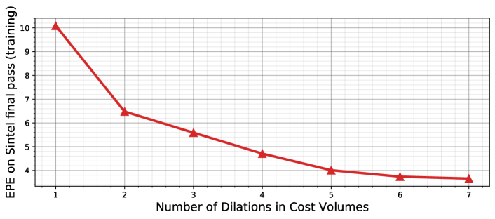
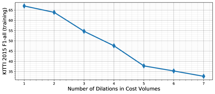
Effectiveness of dilation. We first investigate the effectiveness of using dilation for the cost volume. We vary the number of dilation rates from 7 to 1. To maintain the capability of capturing large displacement, we keep the largest stride and dilation rate and gradually remove smaller ones. We report error rate vs. number of dilation rates in Fig. 6. We can clearly see that the error rates steadily decrease on both MPI Sintel and KITTI 2015 datasets as number of dilation increases. It validates our core idea of constructing cost volumes with dilations to deal with both small and large displacements simultaneously.

Effectiveness of 3D cost volume filtering. We now study the effectiveness of our proposed 3D convolutions for cost volume filtering. To this end, we train other variants with our DCVNet model by replacing the cost volume filtering model presented in Section 3.2, 3D U-Net, with separable 4D and 2D convolution (including flattening and DICL [30]) counterparts . We keep the shape of input and output of the U-Net the same for all other filtering models. The only differences are thus the choices of the cost volume filtering parts, so we can clearly validate the effectiveness of our proposed solution. As we can see in Table 5, for the separable 4D U-Net, we encounter an out-of-memory (OOM) error due to high GPU memory consumption. For the 2D version by flattening the cost volume, it has twice more parameters than our model and still produces inferior error rates on both Sintel and KITTI 2015. We believe this is mainly due to the flatten operation, which ignores the spatial structure of the cost volume. In contrast, our model partially preserves such a structure. Although 2D convolutions with DICL [30] has the least number of parameters and runs slightly faster, it performs worse than our model and consumes more GPU memory. We increase the number of feature dimensions in the cost volume filtering model (the “2D-L, w/ DICL” variant) until we see an OOM error. The model still does not produce error rates as well as our model and consumes more GPU memory.

We can clearly see that our proposed 3D cost volume filtering is a vital component in our proposed DCVNet in order to have an accurate and compact optical flow model with reasonable GPU memory consumption.

Table 5: Comparison of different cost volume filtering methods. Our proposed 3D cost volume filtering achieves a good balance between accuracy, inference speed, and memory consumption. (OOM means out of GPU memory during training and amp indicates usage of automatic mixed precision during inference.)

Method	Sintel		K15	#Para.	Mem.	Time
	clean	final	F1-all	(M)	(GB)	(ms)
2D, w/ flatten [27]	3.00	4.02	32.85%	12.15	1.55	14
2D, w/ DICL [30]	5.35	6.40	61.03%	3.00	2.21	12
2D-L, w/ DICL [30]	4.67	5.58	55.13%	4.28	2.88	13
separable 4D [32]	OOM	OOM	OOM	5.05	3.76	16
3D (ours)	2.47	3.66	32.73%	4.94	1.99	14
3D (ours) w/ amp	2.47	3.66	32.73%	4.94	1.68	14

5 Conclusion

In this paper, we presented DCVNet, a dilated cost volume network for optical flow. Our core idea is to use different dilation rates to construct cost volumes to capture both small and large displacements at the same time with a small neighborhood to retain model efficiency. By doing so, our approach no longer relies on the sequential estimation strategy for optical flow, leading to a fast optical flow model. Moreover, current cost volume filtering models suffer from either inferior accuracy, high memory consumption, or large model size. Therefore, we propose using 3D convolutions to address these issues. Experimental results demonstrate that both dilated cost volumes and 3D convolutions are vital components in our model. Compared to existing approaches, our approach is not only significantly faster but also compact and achieves on-par accuracy on standard benchmarks.

Appendix A Network Architecture of DCVNet

The overall architecture of our proposed DCVNet is illustrated in Fig. 4. It consists of three major components: feature extraction for input images, cost volume filtering with a 3D U-Net, and optical flow hypotheses fusion and upsample. We will introduce each of them in this section.

Figure 7: Network architecture of the image encoder. There are two output at stride of 2 and 8 with dimensions of 128 and 256, respectively.

A.1 Image Encoder

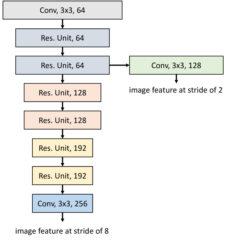
The architecture of the image encoder is shown in Fig. 7. We use a single encoder following the lightweight ResNet architecture [8] used in [28]. The image encoder uses Instance Normalization [29] layers, which are more effective at capturing instance-level correspondences to build the dilated cost volumes. There are two output for the image encoder at stride of 2 and 8 with dimensions of 128 and 256, respectively.

Figure 8: Network architecture of the 3D U-Net for cost volume filtering. An intersection of two arrows indicates concatenation of two feature maps.

A.2 3D U-Net for Cost Volume Filtering

We use a U-Net [24] with 3D convolutions for cost volume filtering, whose network architecture is shown in Fig. 8. We insert an ASPP (Atrous Spatial Pyramid Pooling) module [5] in the bottleneck, where the dilation rates are 2, 4, and 8. It takes the dilated cost volumes with a shape of $C^{\prime}\times D^{\prime}\times\frac{H}{8}\times\frac{W}{8}$, where $C^{\prime}=D\times C$. $D$ is the number of dilation rates ($D=7$ in this paper) and $C$ is the output dimension of the similarity of two feature vectors ($C=4$, see the main paper for details). $D^{\prime}=U\times V$, where $U=V=2k+1$ and $k$ is the neighborhood radius for the cost volume ($k=4$ in this paper so $U=V=9$ and $D^{\prime}=81$). $H$ and $W$ are the height and width of input images, respectively. The output of the 3D U-Net has a shape of $D\times D^{\prime}\times\frac{H}{8}\times\frac{W}{8}$.

A.3 Optical Flow Hypotheses Fusion and Upsample

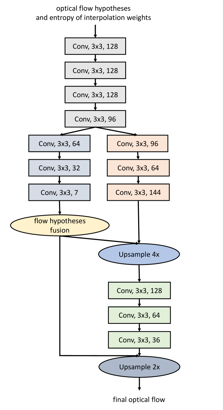
The network architecture for optical flow hypotheses fusion and upsample is shown in Fig. 9. For the hypotheses fusion purpose, we use a set of convolution layers to learn pixel-wise fusion weights for $D$ optical flow hypotheses. See Eq.(4) and Fig.3 in the main paper for the mathematical definition of hypotheses fusion.

The fused optical flow has a spatial resolution of $\frac{H}{8}\times\frac{W}{8}$. To obtain the same resolution as the input, we perform upsampling by 4x and 2x in a cascade manner. For the upsampling block, we train convolutional layers to estimate upsampling weights, which will be used for convex combinations of each position’s neighboring values in a $3\times 3$ grid as used in [28].

Figure 9: Network architecture for optical flow hypotheses fusion and upsample. Blocks denoted by ovals do not have learnable parameters. Each upsample block takes an input tensor and weights for convex combination of neighboring values in a $3\times 3$ grid as used in [28].

Appendix B Visual Results of Optical Flow

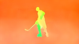
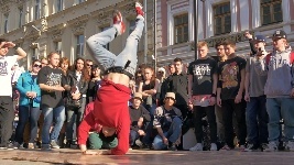
We show more visual results of estimated optical flow from different approaches for MPI Sintel [3] in Fig. 10 and Fig. 11. For KITTI 2015 [21], optical flow results are shown in Fig. 12 and Fig. 13. The results of KITTI 2012 are shown in Fig. 14. We also show optical flow results of our DCVNet on the DAVIS [22] dataset in Fig. 15 to demonstrate the cross-dataset generalization of our approach.

(a) input images	(b) PWCNet [27]	(c) VCN [32]	(d) RAFT [28]	(e) our DCVNet

Figure 10: Visual comparison of optical flow estimations on Sintel. For each method, we show colorized optical flow and error maps (obtained from online servers). For the error maps, white indicates large error while black means small error. Best viewed in color.

(a) input images	(b) HD3 [33]	(c) LiteFlowNet3 [11]	(d) DICL [30]	(e) our DCVNet

Figure 11: Visual comparison of optical flow estimations on Sintel. For each method, we show colorized optical flow and error maps (obtained from online servers). For the error maps, white indicates large error while black means small error. Best viewed in color.

(a) input images	(b) PWCNet [27]	(c) VCN [32]	(d) RAFT [28]	(e) our DCVNet

Figure 12: Visual comparison of optical flow estimations on KITTI 2015. For each method, we show colorized optical flow and error maps (obtained from online servers). For the error maps, red indicates large error while blue means small error. Best viewed in color.

(a) input images	(b) HD3 [33]	(c) LiteFlowNet3 [11]	(d) DICL [30]	(e) our DCVNet

Figure 13: Visual comparison of optical flow estimations on KITTI 2015. For each method, we show colorized optical flow and error maps (obtained from online servers). For the error maps, red indicates large error while blue means small error. Best viewed in color.

(a) input images	(b) PWCNet [27]	(c) HD3 [33]	(d) LiteFlowNet3 [11]	(e) our DCVNet

Figure 14: Visual comparison of optical flow estimations on KITTI 2012. For each method, we show colorized optical flow and error maps (obtained from online servers). For the error maps, white indicates large error while black means small error. Red denotes all occluded pixels, falling outside the image boundaries. Best viewed in color.

(a)	(b)	(c)

Figure 15: Visual results of estimated optical flow for the DAVIS [22] dataset. From left to right: (a) first input images, (b) second input images, and (c) estimated optical flow. The last three rows are failure cases.

References

- [1] Simon Baker, Daniel Scharstein, J. P. Lewis, Stefan Roth, Michael J. Black, and Richard Szeliski. A database and evaluation methodology for optical flow. IJCV, 92(1):1–31, 2011.
- [2] Aviram Bar-Haim and Lior Wolf. Scopeflow: Dynamic scene scoping for optical flow. In CVPR, 2020.
- [3] D. J. Butler, J. Wulff, G. B. Stanley, and M. J. Black. A naturalistic open source movie for optical flow evaluation. In Proc. ECCV, 2012.
- [4] Rohan Chabra, Julian Straub, Christopher Sweeney, Richard A. Newcombe, and Henry Fuchs. Stereodrnet: Dilated residual stereonet. In CVPR, 2019.
- [5] Liang-Chieh Chen, George Papandreou, Iasonas Kokkinos, Kevin Murphy, and Alan L. Yuille. Deeplab: Semantic image segmentation with deep convolutional nets, atrous convolution, and fully connected crfs. IEEE Trans. Pattern Anal. Mach. Intell., 40(4):834–848, 2018.
- [6] Alexey Dosovitskiy, Philipp Fischery, Eddy Ilg, Caner Hazirbas, Vladimir Golkov, Patrick van der Smagt, Daniel Cremers, Thomas Brox, et al. FlowNet: Learning optical flow with convolutional networks. In Proc. ICCV, 2015.
- [7] Andreas Geiger, Philip Lenz, and Raquel Urtasun. Are we ready for autonomous driving? the kitti vision benchmark suite. In Proc. CVPR, pages 3354–3361. IEEE, 2012.
- [8] Kaiming He, Xiangyu Zhang, Shaoqing Ren, and Jian Sun. Deep residual learning for image recognition. In Proc. CVPR, 2016.
- [9] B.K.P. Horn and B.G. Schunck. Determining optical flow. Artificial Intelligence, 1981.
- [10] Tak-Wai Hui, Xiaoou Tang, and Chen Change Loy. A lightweight optical flow cnn - revisiting data fidelity and regularization. IEEE Trans. on Pattern Anal. and Mach. Intell., 2020.
- [11] Tak-Wai Hui and Chen Change Loy. Liteflownet3: Resolving correspondence ambiguity for more accurate optical flow estimation. In ECCV, 2020.
- [12] Tak-Wai Hui, Xiaoou Tang, and Chen Change Loy. Liteflownet: A lightweight convolutional neural network for optical flow estimation. In Proc. CVPR, 2018.
- [13] Eddy Ilg, Nikolaus Mayer, Tonmoy Saikia, Margret Keuper, Alexey Dosovitskiy, and Thomas Brox. FlowNet 2.0: Evolution of optical flow estimation with deep networks. In Proc. CVPR, 2017.
- [14] Eddy Ilg, Tonmoy Saikia, Margret Keuper, and Thomas Brox. Occlusions, motion and depth boundaries with a generic network for disparity, optical flow or scene flow estimation. In Proc. ECCV, 2018.
- [15] Huaizu Jiang, Deqing Sun, Varun Jampani, Zhaoyang Lv, Erik G. Learned-Miller, and Jan Kautz. SENSE: A shared encoder network for scene-flow estimation. In ICCV, 2019.
- [16] Diederik P. Kingma and Jimmy Ba. Adam: A method for stochastic optimization. In Proc. ICLR, 2015.
- [17] D. Kondermann, R. Nair, K. Honauer, K. Krispin, J. Andrulis, A. Brock, B. Güssefeld, M. Rahimimoghaddam, S. Hofmann, C. Brenner, and B. Jähne. The hci benchmark suite: Stereo and flow ground truth with uncertainties for urban autonomous driving. In CVPRW, 2016.
- [18] Yao Lu, Jack Valmadre, Heng Wang, Juho Kannala, Mehrtash Harandi, and Philip Torr. Devon: Deformable volume network for learning optical flow. In WACV, March 2020.
- [19] Nikolaus Mayer, Eddy Ilg, Philip Häusser, Philipp Fischer, Daniel Cremers, Alexey Dosovitskiy, and Thomas Brox. A large dataset to train convolutional networks for disparity, optical flow, and scene flow estimation. In CVPR, 2016.
- [20] Moritz Menze and Andreas Geiger. Object scene flow for autonomous vehicles. In Proc. CVPR, pages 3061–3070, 2015.
- [21] Moritz Menze, Christian Heipke, and Andreas Geiger. Object scene flow. ISPRS Journal of Photogrammetry and Remote Sensing (JPRS), 2018.
- [22] F. Perazzi, J. Pont-Tuset, B. McWilliams, L. Van Gool, M. Gross, and A. Sorkine-Hornung. A benchmark dataset and evaluation methodology for video object segmentation. In CVPR, 2016.
- [23] Anurag Ranjan and Michael J Black. Optical flow estimation using a spatial pyramid network. In Proc. CVPR, 2017.
- [24] Olaf Ronneberger, Philipp Fischer, and Thomas Brox. U-net: Convolutional networks for biomedical image segmentation. In MICCAI, 2015.
- [25] Karen Simonyan and Andrew Zisserman. Two-stream convolutional networks for action recognition in videos. In NeurIPS, 2014.
- [26] Leslie N. Smith and Nicholay Topin. Super-convergence: Very fast training of residual networks using large learning rates. CoRR, abs/1708.07120, 2017.
- [27] Deqing Sun, Xiaodong Yang, Ming-Yu Liu, and Jan Kautz. Pwc-net: Cnns for optical flow using pyramid, warping, and cost volume. In CVPR, June 2018.
- [28] Zachary Teed and Jia Deng. RAFT: recurrent all-pairs field transforms for optical flow. In ECCV, 2020.
- [29] Dmitry Ulyanov, Andrea Vedaldi, and Victor S. Lempitsky. Instance normalization: The missing ingredient for fast stylization. CoRR, abs/1607.08022, 2016.
- [30] Jianyuan Wang, Yiran Zhong, Yuchao Dai, Kaihao Zhang, Pan Ji, and Hongdong Li. Displacement-invariant matching cost learning for accurate optical flow estimation. In NeurIPS, 2020.
- [31] Taihong Xiao, Jinwei Yuan, Deqing Sun, Qifei Wang, Xin-Yu Zhang, Kehan Xu, and Ming-Hsuan Yang. Learnable cost volume using the cayley representation. In ECCV, 2020.
- [32] Gengshan Yang and Deva Ramanan. Volumetric correspondence networks for optical flow. In NeurIPS, 2019.
- [33] Zhichao Yin, Trevor Darrell, and Fisher Yu. Hierarchical discrete distribution decomposition for match density estimation. In CVPR, 2019.
- [34] Shengyu Zhao, Yilun Sheng, Yue Dong, Eric I-Chao Chang, and Yan Xu. Maskflownet: Asymmetric feature matching with learnable occlusion mask. In CVPR, 2020.