Finding optimal Bell inequalities using the cone-projection technique

Abstract

Bell inequalities are relevant for many problems in quantum information science, but finding them for many particles is computationally hard. Recently, a computationally feasible method called cone-projection technique has been developed to find all optimal Bell inequalities under some constraints, which may be given by some symmetry or other linear conditions. In this paper we extend this work in several directions. We use the method to generalize the I4422 inequality to three particles and a so-called GYNI inequality to four particles. Additionally, we find Bell inequalities for three particles that generalize the I3322 inequality and the CHSH inequality at the same time. We discuss the obtained inequalities in some detail and characterize their violation in quantum mechanics.

I Introduction

Bell inequalities are a tool to test whether experimental data is compatible with a local hidden variable (LHV) model or not Brunner et al. (2014); Scarani (2019). Quantum mechanics predicts that Bell inequalities can be violated and this has been verified experimentally in an unambiguous manner Shalm et al. (2015); Hensen et al. (2015); Giustina et al. (2015); Rosenfeld et al. (2017). The violation of a Bell inequality requires the presence of entanglement, so Bell inequalities provide the possibility to detect entanglement in a device-independent manner. This can be extended to certify certain quantum states and measurements, by a procedure called self-testing Šupić and Bowles (2020). Moreover, in quantum cryptography Bell inequality violations can certify secret-key rates Holz et al. (2019). All these applications exemplify that the violation of a Bell inequality can be useful. Even beyond that, some Bell inequalities can be interesting if they cannot be violated by quantum mechanics. Indeed, in this case they may distinguish quantum mechanics from more general non-signaling theories Almeida et al. (2010). The wide range of applications of Bell inequalities beyond their original purpose of refuting LHV theories makes it desirable to find Bell inequalities with interesting properties.

This, however, is an arduous endeavour as the correlations stemming from LHV models form a high-dimensional polytope and identifying interesting Bell inequalities amounts to finding the corresponding facets of this local polytope Peres (1999). Finding the facets of a high-dimensional polytope given its extreme points is known to be a hard task and its computational complexity quickly renders it intractable as the number of parties, measurements per party or outcomes per measurement rise Pitowsky (1991).

Furthermore, the number of facet-defining Bell inequalities increases rapidly, making it difficult to identify the inequalities of interest. To give an example, there are only eight non-trivial Bell inequalities all of which are versions of the famous Clauser-Horne-Shimony-Holt (CHSH) inequality Clauser et al. (1969, 1970) in the scenario with two parties and two different dichotomic measurements per party each. For the same number of parties, but three dichotomic measurements per party, there are already 648 non-trivial facet-defining inequalities, 72 of which are of the CHSH type and 576 are variations of the so-called I3322 inequality. The latter inequality was first identified by Froissart Froissart (1981) and later independently by Śliwa Śliwa (2003) and Collins and Gisin Collins and Gisin (2004). If one increases the number of parties, for three parties with two dichotomic measurements each, there are 53856 facet-defining inequalities and 46 inequivalent classes of Bell inequalities Śliwa (2003). Going to even more complex scenarios it is impossible so far to compute all the facets.

Luckily however, in practice we rarely need a complete characterization of the local polytope. Instead, we seek Bell inequalities with properties that are suitable for a specific purpose. In a recent work Bernards and Gühne (2020) we proposed a general method for this problem. Henceforth we refer to this method as the cone-projection technique (CPT). The CPT can be used to find all optimal Bell inequalities obeying some affine constraints. Specifically, one important task that can be addressed with the CPT is finding generalizations of a Bell inequality.

In this paper we present a an extended description of the CPT and use it then to study several scenarios. First, we present a detailed analysis of the properties of three-particle generalizations of the I3322 inequality previously found Bernards and Gühne (2020). Second, we study generalization of the so-called I4422 inequality Collins and Gisin (2004) to three particles. Third, we find and investigate three-particle Bell inequalities that are generalizations of the CHSH inequality and the I3322 inequality at the same time. Finally, we study generalizations of three-particle Guess-Your-Neighbors-Input (GYNI) inequality Almeida et al. (2010) to four particles.

Before embarking into the technical description of the CPT and the examples, it may be useful to explain the notion of a generalization of a Bell inequality to more particles. Let us consider an example. Mermin’s inequality, which reads

$$\langle{A_{1}B_{1}C_{2}}\rangle+\langle{A_{1}B_{2}C_{1}}\rangle+\langle{A_{2}B_{1}C_{1}}\rangle-\langle{A_{2}B_{2}C_{2}}\rangle\leq 2$$ (1)

can be seen as a generalization of the CHSH inequality

$$\langle{A_{1}B_{1}}\rangle+\langle{A_{1}B_{2}}\rangle+\langle{A_{2}B_{1}}\rangle-\langle{A_{2}B_{2}}\rangle\leq 2.$$ (2)

This should be understood in the following way: If Charlie fixes his outcomes $\pm 1$ for the measurements $C_{1}$ and $C_{2}$ deterministically (instead of performing an actual measurement) then Alice and Bob perform essentially a CHSH test on the two-body marginal of the shared three-party state. Specifically, if we insert $C_{1}=C_{2}=1$ into Mermin’s inequality, it reduces to the CHSH inequality. We therefore say that Mermin’s inequality is reducible to the CHSH inequality. Moreover, both the CHSH inequality and the Mermin inequality are define facets on the local polytope. Both properties combined make the Mermin inequality a generalization of the CHSH inequality. In some situations, these two conditions are too weak to find all the Bell inequalities that satisfy them, then one may impose some symmetry constraints in addition; this can also be handled by the CPT. In the above example one may for instance impose invariance under arbitrary permutations of parties.

II Description of the cone-projection technique (CPT)

In this section, we provide a detailed description of the method presented in Ref. Bernards and Gühne (2020). The reader who is already familiar with it may directly skip to the next section.

Figure 1: A polytope in three-dimensional space is defined by its two-dimensional surfaces, the so-called facets. Here, the normal vectors of the facets are depicted as blue vectors. The vector $\bm{g}$ (black arrow) may be used to define a condition on the facets, be requiring that the facet normal vectors $\bm{f}_{i}$ must enclose some absolute angle $\alpha$. For instance, this angle may be chosen such that the facets drawn in green meet the constraints while the others drawn in orange do not.

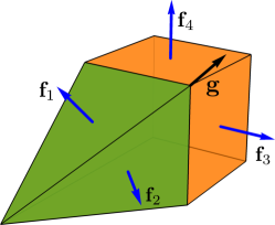
II.1 Overview and motivation

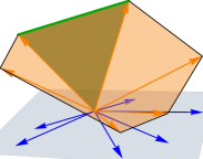
We wish to find a method that allows to compute facets of a polytope which is defined by its vertices, where the facet normal vectors obey some linear constraints. This can be interpreted geometrically as the condition that the facet normal vectors must have a fixed inner product with some vector $\bm{g}$ that represents the condition, see also Fig. 1. A naive method to tackle this problem is to compute first all facets and then to find out which of them obey the constraint. For the problems we consider, however, this is not feasible, as it is already impossible to compute all the facets.

Note that constraints of the considered type include two important special cases of constraints that are important in this work: The condition that some given vertex of the polytope should lie on the desired facet and the condition that the normal vector should be symmetric under some linear transformation. In the first case, the position vector of the vertex in question takes the role of $\bm{g}$. To understand this, consider a Bell inequality $\bm{x}^{T}\bm{b}\leq-\beta$ with facet normal vector $\bm{b}$ that should hold for all classical behaviors $\bm{x}$. Demanding that some vertex $\bm{g}$ lies on the facet means that $\bm{g}^{T}\bm{b}=-\beta$, which is an affine constraint. In the second case all points that obey the symmetry lie in a plane and the normal vectors of the desired facets have to lie in this plane as well. This is illustrated in Fig. 2.

Figure 2: This example shows how symmetries can be formulated as affine constraints. We seek facets with normal vectors that are invariant under reflection on a plane (white, half-transparent). This is satisfied by the normal vectors $\bm{f}_{1},\bm{f}_{2}$ (blue) of two of the facets (green). The condition is equivalent to demanding that the normal vectors be perpendicular to the normal vectors (black arrows) of the mirror plane.

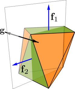
II.2 Description of convex cones and polytopes

For formulating the method in a precise manner, we need some more terminology Ziegler (1995). In detail, we need to define the notions of polytopes, cones and polyhedra, as well as their so-called V-representation and H-representation. Finally, we define facets and discuss the dimensions of these objects.

The two most fundamental concepts in this context are conic combinations and convex combinations. Conic combinations are linear combinations with positive coefficients. Convex combinations are linear combinations with positive coefficients where the coefficients sum up to one. Given a set $V$ of vectors, the set of all conic (convex) combinations of the elements in $V$ is called the conic (convex) hull of $V$. Also, the conic (convex) hull of $V$ is said to be generated by $V$ under conic (convex) combinations. If $V$ is finite, its convex hull is called finitely generated.

These notions give rise to the two main objects that are studied in the following, convex cones and convex polytopes. The first are assumed to be finitely generated under conic combinations and the second being finitely generated under convex combinations. The elements of $V$ are called vertices in the case of polytopes. For cones, they are called rays.

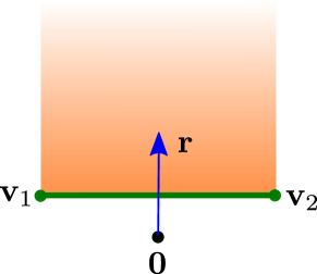
The notion of polytopes and cones can be unified using the concept of polyhedra. First, given two sets $A$ and $B$, one can define their so-called Minkowski sum as $A+B=\{a+b|a\in A,b\in B\}$. The sum of a cone and a polytope is called a polyhedron. The sets of rays and vertices that generate the polyhedron are called the V-representation of the polyhedron. Fig. (3) illustrates the Minkowski sum of a line segment and a ray.

Figure 3: The vertices $\bm{v}_{1}$, $\bm{v}_{2}$ (green points) define a 1-dimensional polytope (green bold line). The Minkowski sum of this polytope and the ray $\bm{r}$ (blue) is a polyhedron (orange), which extends infinitely to the top. The polyhedron has three facets, which are the lines that confine it to the bottom, the left, and the right.

That said, there is a second important representation of polyhedra, the H-representation. Any polyhedron can be viewed as the intersection of a finite number of half-spaces, defined by affine inequalities. The minimal set of half-spaces whose intersection is the polyhedron is its H-representation.

Let us finally introduce the concept of a facet. With every of the half-spaces in the H-representation, we can associate the hyperplane that bounds it. The intersection between such a hyperplane and the polyhedron is called a facet of the polyhedron. If an inequality defines a half-space such that its bounding hyperplane contains a facet of a given polyhedron, this inequality is called facet-defining with respect to the polyhedron. From a physical perspective, such facet-defining inequalities are the most interesting Bell inequalities.

If a polyhedron $P$ has dimension $D$, its facets are the $D-1$ dimensional polyhedra that together form the boundary of $P$. Intersections of facets are called faces. In the following, an $n$-face is a face that has an (affine) dimension of $n$. Accordingly, in the case of a $D$ dimensional polytope, $0$-faces are vertices, $1$-faces are edges and $(D-1)$-faces are facets.

II.3 Targeted search for facets

Now we are in the position to describe the problem that the cone-projection technique described in Ref. Bernards and Gühne (2020) solves. We consider the situation where a convex polytope $P$ is given in its V-representation and we aim to find all facets of $P$ that satisfy some linear conditions. The CPT works for the case that the conditions are affine equality constraints on the coefficients of the facet defining inequality. Note that the CPT can be applied to any convex polyhedron, but in practice we are interested in the local polytope, where the vertices are given by deterministic assignments of measurement results in a LHV model.

(a)

(b)

(c)

(d)

Figure 4: Visualization of the CPT to find facets of a polytope where the normal vector obeys some constraints. (a) We aim to find the facets of the two-dimensional polytope $P$ where the normal vector $\bm{b}_{P}$ has a fixed scalar product with some vector $\bm{g}$. The facet and the normal vector that fulfill this constraint in the given example are shown in green. (b) We embed the polytope $P$ in a plane in three-dimensional space, where the plane does not contain the origin $\bm{0}$. The vertices of $P$ define rays (orange arrows) that define the cone $C$. The polytope $P$ is then the intersection of the cone $C$ with the plane, and each of its facets relates to a facet of $C$ (green) in a unique manner. (c) The initial constraint on the facet of $P$ can be translated to conditions on the facets of the cone. A facet of $P$ fulfills the constraint if and only if the corresponding facet of $C$ has a normal vector $\bm{b}_{C}$ that obeys a linear constraint $G\bm{b}_{C}=0$, where $G$ is some matrix. Geometrically, this means that $\bm{b}_{C}$ has to lie in a certain plane (light-grey). Then, we project the rays of $C$ (orange) into that plane (blue arrows) to define a cone $\widetilde{C}$ in the low-dimensional plane by taking projected rays as generators. By construction, facets of $C$ which obey the constraint are also facets of the projected cone $\widetilde{C}$. (d) Finally, we find the facets of $\widetilde{C}$ and check which ones correspond to facets of $C$. From the facets of $C$ that meet the conditions we can then compute the corresponding facets of $P$. In our example, $\widetilde{C}$ is a half plane (light-blue) and has only one facet with the normal vector in green. It is also the normal vector of a facet of $C$ (green). Note that in the given example $\widetilde{C}$ is already generated by three rays and the other three rays are redundant.

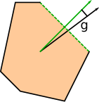
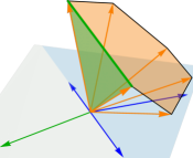
We consider a $D$-dimensional polytope $P$ and affine conditions on the facet normal vectors. Each of these conditions can be written in the form

$$\bm{g}^{T}_{k}\bm{b}_{P}=\gamma_{k},$$ (3)

that is, the normal vector $\bm{b}_{P}$ has a fixed scalar product with some vector $\bm{g}_{k}$, see Fig. 4(a). The task is to find all the facet normal vectors that obey these constraints.

In the first step, we construct a cone $C$ in $D+1$-dimensional space that maintains a one-to-one correspondence to the polytope. One way to achieve this is to prepend one fixed coordinate to every vertex $\bm{v}_{i}$,

$$\bm{v}_{i}\mapsto\bm{w}_{i}=\binom{1}{\bm{v}_{i}}.$$ (4)

and to define the cone $C$ as the conic hull of the rays $\bm{w}_{i}$. In this way, the polytope can be seen as the intersection of the cone $C$ with the hyperplane defined by $x_{0}=1$. This relationship is illustrated in Fig. 4(b). Notably, there is a one-to-one correspondence between the facets of the cone and those of the polytope, and a normal vector $\bm{b}_{P}$ of a polytope facet translates to a normal vector $\bm{b}_{C}$ of a cone facet. This is easy to formulate in the H-representation of the polytope and the corresponding cone. Let

$$\bm{x}^{T}\bm{b}_{P}\leq-\beta$$ (5)

be a facet-defining inequality of the polytope. Then,

$$(1\;\bm{x}^{T})\binom{\beta}{\bm{b}_{P}}\leq 0$$ (6)

is the corresponding facet-defining inequality of the cone. Note that then $\binom{\beta}{\bm{b}_{P}}$ is the normal vector of the facet, and any normal vector of a facet can be written in this way.

The correspondence between the polytope and the cone enables us to work with the cone instead of the polytope. This construction also allows to write the conditions in Eq. (3) in a linear form, namely

$$(g_{0,k}\;\bm{g}^{T}_{k})\binom{\beta}{\bm{b}_{P}}=0,$$ (7)

where we set $g_{0,k}=-\frac{\gamma_{k}}{\beta}$.

Collecting all the facet conditions yields the linear matrix equation

$$G\bm{b}_{C}=0,$$ (8)

where the $k$-th row of $G$ is the row vector $(g_{0,k}\;\bm{g}^{T}_{k})$ and the facet normal vector of the cone is $\bm{b}_{C}=\binom{\beta}{\bm{b}_{P}}$. Geometrically speaking, Eq. (8) defines a hyperplane through the origin in which the facet normal vectors of the cone must lie in order to comply with the conditions in Eq. (3), see also Fig. 4(c).

The key observation is that in this situation we can define a new cone $\widetilde{C}$, such that if $\bm{b}_{C}$ is a facet normal vector of $C$ that obeys the constraints, then $\bm{b}_{C}$ is also a facet normal vector of $\widetilde{C}$. This is done by projecting the rays of $C$ down to the subspace of vectors obeying $G\bm{v}=0$, see Fig. 4(c) and Fig. 5.

Figure 5: Detailed view of the of the projection of the rays of the cone $C$ onto the plane where $G\bm{b}_{C}=0$. The projected rays (in blue) generate a new cone $\widetilde{C}$. Depending on the conditions, this new cone may have a significantly reduced dimension compared with $C$.

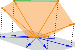
This subspace is the kernel of $G$ and it is spanned by a set of $K$ vectors $\bm{t}_{i}$, where $K$ is the dimension of the kernel. The advantage of $\widetilde{C}$ is that its dimension $K$ is typically considerably smaller than the dimension of $C$. Additionally, $\widetilde{C}$ has typically much less rays than $C$. That makes it easier to find all the facets of $\widetilde{C}$, compared with $C$, see Fig. 4(d).

In practice, the first step in the construction of $\widetilde{C}$ is to define the $(D+1)\times K$ matrix $T$, whose $K$ columns of length $D+1$ are given by the vectors $\bm{t}_{j}$, so we have $T_{ij}=[\bm{t}_{j}]_{i}$. With this, we define the rays of $\widetilde{C}$ as

$$\bm{\widetilde{w}_{i}}^{T}=\bm{w_{i}}^{T}T.$$ (9)

Note that this is a projection if the vectors $\bm{t}_{j}$ form an orthonormal basis of the kernel of $G$. However, this is in general not necessary and in practice it can be preferable to pick vectors $\bm{t}_{j}$ with integer coefficients, so that the rays of $\widetilde{C}$ have integer coefficients, if the rays of $C$ have integer coefficients. In this way, one does not need to worry about the precision of the numerical calculations.

Similarly to the rays of $C$, we can express its facet normal vectors $\bm{b}_{C}$ (that satisfy the constraints) in the basis $\bm{t}_{j}$ of the kernel of $G$ as

$$\bm{b}_{C}=T\bm{b}_{\widetilde{C}},$$ (10)

where $\bm{b}_{\widetilde{C}}$ is a vector of dimension $K$.

The following theorem is the central result and establishes the previously claimed relation between $\widetilde{C}$ and $C$. Namely, it states that any time $\bm{b}_{C}$ is a facet normal vector of $C$ that satisfies the conditions, $\bm{b}_{\widetilde{C}}$ is a facet normal vector of $\widetilde{C}$. In this way, the facet normal vectors of $\widetilde{C}$ are the only relevant vectors that one needs to consider.

Theorem 1.

Let $C=\text{conv}(\{\bm{w}_{i}\})$ be a cone and $\bm{b}_{C}$ a facet normal vector of $C$ that satisfies $G\bm{b}_{C}=0$ for some matrix $G$. With $T$ and $\bm{b}_{\widetilde{C}}$ defined as above, we define the cone $\widetilde{C}=\text{conv}(\{\bm{\widetilde{w}_{i}}\})$ of dimension $K$ with $\bm{\widetilde{w}_{i}}^{T}=\bm{w_{i}}^{T}T$. Then $\bm{b}_{\widetilde{C}}$ defines a facet of $\widetilde{C}$.

Proof.

We prove the statement in three steps. (1) The inequality $\bm{\widetilde{w}_{i}}^{T}\bm{b}_{\widetilde{C}}\leq 0$ holds, since Eq. (10) together with the definition of the $\bm{\widetilde{w}_{i}}$ implies

$$\bm{\widetilde{w}_{i}}^{T}\bm{b}_{\widetilde{C}}=\bm{w_{i}}^{T}\bm{b}_{C}$$ (11)

and $\bm{w_{i}}^{T}\bm{b}\leq 0$ because $\bm{b}_{C}$ is facet defining.

(2) The vector $\bm{b}_{\widetilde{C}}$ defines a face of $\widetilde{C}$, as one can directly see from Eq. (11). With $K=\dim(\ker G)$, the dimension of the face is at most $K-1$, since it is contained in the $K-1$ dimensional subspace $\{\bm{x}\,|\,\bm{x}^{T}\bm{b}_{\widetilde{C}}=0\}$.

(3) The vector $\bm{b}_{\widetilde{C}}$ defines a facet of $\widetilde{C}$. That is, the dimension of the face is exactly $K-1$.

Let $B$ be the $M\times(D+1)$ matrix that contains all M rays $\bm{w}_{i}$ as rows that fulfill $\bm{w}_{i}^{T}\bm{b}_{C}=0$. Since $\bm{b}_{C}$ is a facet normal vector, $B$ has rank $D$. Accordingly, $BT$ is the $M\times K$ matrix that contains all rays $\bm{\widetilde{w}_{i}}^{T}$ as rows that fulfill $\bm{\widetilde{w}_{i}}^{T}\bm{b}_{\widetilde{C}}=0$. Showing that $\bm{\widetilde{b}}$ defines a facet is equivalent to showing that $\text{rank}(BT)=K-1$. We now prove the latter by contradiction. Assume there exist two linearly independent vectors $\bm{\widetilde{b}},\bm{\widetilde{c}}$ that satisfy $BT\bm{\widetilde{b}}=BT\bm{\widetilde{c}}=0$. Thus, $T\bm{\widetilde{b}}$ and $T\bm{\widetilde{c}}$ lie in the kernel of $B$. Since $\text{rank}(B)=D$, the kernel is one-dimensional, so we can write $T\bm{\widetilde{c}}=\ell T\bm{\widetilde{b}}$ for some real number $\ell$. This implies $T(\bm{\widetilde{c}}+\ell\bm{\widetilde{b}})=0$. Because $\bm{\widetilde{b}}$ and $\bm{\widetilde{c}}$ are linearly independent, the kernel of $T$ has at least dimension one, which is impossible because $T$ has full column rank. ∎

The facets of interest of the polytope $P$ can now be found by finding the facets of $\widetilde{C}$ first, calculating potential facets of $C$ via Eq. (10), transforming these into potential facets of $P$ and finally checking which of the found inequalities define facets of $P$. Note that it is computationally simple to check whether a given candidate is a facet, one just needs to compute the dimension of the surface.

II.4 Some facts about the local polytope

After discussing polytopes in general we should also address the class of polytopes of interest in this paper, namely local polytopes. The aim of a Bell test is to discriminate between classical and non-classical behaviors. As the name suggests, the behavior of a system in a Bell test captures the relevant data from the Bell test experiment. A behavior is a vector consisting of so-called correlations. In general, a correlation is the conditional probability of some combination of local measurement outcomes given a combination of local measurements that are performed in a time-like separated manner. This includes the case that some parties may not perform any measurement on their subsystem, in which case the measured correlation is called a marginal correlation, in contrast to a full-body correlation, which captures the case in which every party performs a non-trivial measurement.

Note that there is no need to consider the conditional probabilities for all possible combinations of outcomes given a combination of local measurement settings. The reason for this is that there are two rules that hold for the behaviors. The first rule is that the probabilities for the different combinations of local measurement outcomes given the same local measurement settings will sum up to one. The second rule is the no-signaling principle. It states that the probability for any local measurement outcome does not depend on the choices for the measurement settings on the other subsystems. This reduces the dimension of a behavior to

$$D(n,\bm{m},o)=\prod_{i=1}^{n}\left(\sum_{j=1}^{m_{i}}(o_{ij}-1)+1\right)-1,$$ (12)

where $n$ denotes the number of parties, $m_{i}$ is the number of measurement settings of party $i$ and $o_{ij}$ is the number of possible measurement outcomes for setting $j$ of party $i$ Pironio (2005). The numbers $n,m_{i},o_{ij}$ define a so-called scenario for a Bell test. All scenarios considered in this paper feature dichotomic measurements exclusively, so $o_{ij}=2,\;\forall i,j$.

In this case it is sufficient to consider the expectation value of the product of a combination of local measurement outcomes, given the measurement settings as a correlation instead of a conditional probability. One readily verifies that this leads to the correct number of independent correlations according to Eq. (12).

Classical behaviors behave in accordance with a local hidden variable (LHV) model. In a LHV model, the local measurement outcomes are fundamentally predetermined by a local hidden variable $\lambda$. However, if the local hidden variable takes on different values through different runs of an experiment, this will cause the observed behavior to be a mixture of the local deterministic behaviors. Mathematically speaking, the classical behaviors lie in a polytope, the local polytope, which is defined as the convex hull of its vertices, the local deterministic behaviors. Therefore, in order to define the local polytope for a specific scenario, one must enumerate all local deterministic behaviors, where each local deterministic behavior corresponds to one combination of local deterministic assignments of a measurement outcome to each measurement setting, yielding

$$N=\prod_{i,j}o_{ij}$$ (13)

vertices in total.

III Results

In this section, we present detailed results on generalizations of existing Bell inequalities to more parties using the cone-projection technique. We start with general considerations, then we present details on the found Bell inequalities for four relevant scenarios.

III.1 General considerations

For simplicity, we only consider Bell inequalities for scenarios in which every measurement has two possible outcomes. This allows us to write the Bell inequalities in a notation using observables. To simplify the notation of Bell inequalities that include marginal terms, that is, correlations that do not involve all parties, we define the zeroth setting of every party to refer to a measurement that always yields the result $1$. Hence, $\langle A_{1}\rangle$ is equivalent to $\langle A_{1}B_{0}C_{0}...\rangle$. Moreover, this allows us to write any three-party Bell inequality in the form $\sum_{ijk}b_{ijk}\langle A_{i}B_{j}C_{k}\rangle\geq 0$, where $b_{000}$ accounts for the constant term.

As we already explained in the introduction, we call a facet-defining $(n+1)$-party Bell inequality that is reducible to an $n$-party Bell inequality a generalization of the latter. In mathematical terms, we can formulate this condition for a facet-defining bipartite Bell inequality that is to be generalized to a three-party Bell inequality as follows. The three-party Bell inequality $\sum_{i,j,k}b_{ijk}\langle A_{i}B_{j}C_{k}\rangle\geq 0$ is called a generalization of the Bell inequality $\sum_{ij}\beta_{ij}\langle A_{i}B_{j}\rangle\geq 0$ if it is facet-defining and there exist deterministic choices $\xi_{k}\in\{-1,1\}$ for the outcomes of Charlie such that

$$\sum_{i,j,k}b_{ijk}\xi_{k}\langle A_{i}B_{j}\rangle=\sum_{ij}\beta_{ij}\langle A_{i}B_{j}\rangle.$$ (14)

This condition implies the following: If $\gamma$ with $\gamma_{ij}=\langle A_{i}B_{j}\rangle$ is a behavior that saturates the two party Bell inequality, that is $\sum_{ij}\beta_{ij}\gamma_{ij}=0$, then the behavior $g_{ijk}=\gamma_{ij}\xi_{k}$ will saturate its generalization. Since $g$ is a three-party extension of the behavior $\gamma$, we call it an extended behavior.

Note that the condition that the extended behavior should saturate the generalized Bell inequality is a linear constraint and can thus be handled with the CPT. However, there can be generalized Bell inequalities for every possible deterministic choice of assignments of outcomes $\xi_{k}$ to Charlies measurement settings, so we have to find all the generalized Bell inequalities for every of these choices. Fixing one choice, we obtain one extended behavior for every saturating behavior of the inequality we seek to generalize.

Additionally, we require that generalized Bell inequalities should obey symmetries that are characteristic for the inequality they generalize. This narrows down the search and increases the similarity between an inequality and its generalizations.

In the following, we present generalizations of several inequalities that will be discussed in their respective sections. For every inequality we found, we conduct the same numerical analysis. We compute the quantum mechanical violation for qubits, for qutrits and for the second and (if possible) third level of the NPA-hierarchy Navascués et al. (2007). For the latter, we used the ncpol2sdpa package by Peter Wittek Wittek (2015). For the qubit and qutrit violations, we provide lower bounds using a seesaw algorithm that alternates between optimizing the measurement settings of one of the parties and optimizing the state. Every of these optimization steps is a semidefinite program. Details can be found in Appendix A.

For meaningful comparisons between the inequalities, we compute four quantities for every Bell inequality $\langle\mathcal{B}\rangle\ \equiv\sum_{ijk\neq 000}-b_{ijk}\langle A_{i}B_{j}C_{k}\rangle\leq b_{000}$ that will guide the following discussion.

The first quantity is the relative qutrit violation by which the maximal value of the Bell expression $\mathcal{B}$ achievable with qutrits exceeds the maximal classical value. It is defined as

$$m_{Q} =\frac{\max_{\text{qutrit}}\langle\mathcal{B}\rangle}{b_{000}}-1.$$ (15)

We are interested in this quantity as a signature to identify inequalities whose quantum violation is particularly strong. In this regard, it would be more informative to consider the quantum violation with a higher-dimensional system. However, the computations become more demanding which is why we restrict our quantum mechanical analysis to qubit and qutrit systems.

The second quantity we consider is the algebraic-classical ratio that is defined analogously and quantifies, by how much the algebraic maximum of the Bell expression exceeds the classical bound in relation to the classical bound. It is calculated as

$$m_{A} =\frac{\sum_{i,j,k}|b_{ijk}|-b_{000}}{b_{000}}.$$ (16)

As a third interesting quantity, we compute the NPA-qutrit ratio that quantifies the relative margin between the maximal value of the Bell expression in the third level of the NPA hierarchy and the maximal value achievable with qutrits. For some of the Bell inequalities we found, it was unfeasible to compute the third level of the NPA hierarchy. In this situation we resorted to the value obtained by the second level of the NPA hierarchy. Every time this is the case it is stated explicitely. The NPA-qutrit ratio is calculated as

$$m_{N} =\frac{\max_{\text{NPA}}\langle\mathcal{B}\rangle}{\max_{\text{qutrit}}\langle\mathcal{B}\rangle}-1.$$ (17)

Lastly, we consider the qutrit-qubit ratio $m_{32}$ by which the maximal value of the Bell expression $\mathcal{B}$ achieved by qutrits exceeds the corresponding value for qubits. Mathematically, it is defined as

$$m_{32} =\frac{\max_{\text{qutrit}}\langle\mathcal{B}\rangle}{\max_{\text{qubit}}\langle\mathcal{B}\rangle}-1.$$ (18)

It is natural to state these relative margins in percent, in which case $m_{32}=10\%$ means that the maximal value of the Bell expression is $10\%$ larger for qutrit systems than for qubit systems.

In the following, we report those inequalities that exhibit the biggest value for one of the four relative quantities. A big qutrit-qubit ratio $m_{32}$ makes the inequality potentially interesting for experimental discrimination between qubit and qutrit states (i.e. device-independent dimension witnessing), while a large NPA-qutrit ratio $m_{N}$ suggests that the maximal quantum mechanical violation of the inequality may not be achievable with qutrit states. A large relative qutrit violation $m_{Q}$ hints at a particularly strong violation of the inequality in quantum mechanics, while a large algebraic-classical ratio $m_{A}$ shows that observers that play by the rules of classical physics are especially limited in obtaining a large expectation value for the Bell expression in comparison with hypothetical observers who do not suffer any physical limitations.

Finally, while we defined the quantities in this subsection for three parties, all the definitions can easily be extended to four-party Bell inequalities.

III.2 Investigation of I3322 generalizations

The I3322 inequality is the next simplest Bell inequality to consider after the standard CHSH inequality and it is the only facet-defining Bell inequality in the bipartite scenario with three dichotomic measurements per party (besides lifted versions of the CHSH inequality). It reads

$$\langle{A_{1}}\rangle -\langle{A_{2}}\rangle+\langle{B_{1}}\rangle-\langle{B_{2}}\rangle-\langle{(A_{1}-A_{2})(B_{1}-B_{2})}\rangle$$

$$+\langle{(A_{1}+A_{2})B_{3}}\rangle+\langle{A_{3}(B_{1}+B_{2})}\rangle\leq 4.$$ (19)

The I3322 inequality, or I3322 for short, was first discovered by Froissart in 1981 Froissart (1981) and more than twenty years later rediscovered by Sliwa Śliwa (2003) and, independently, Collins and Gisin Collins and Gisin (2004). It has sparked interest because its maximal quantum violation is not achievable with qubits. Curiously, there is no difference in the maximal quantum violations achieved by qubits and qutrits. In fact, the local dimensions of Alice’s and Bob’s must be at least twelve in order to observe a larger quantum violation than the one achievable with qubits Pál and Vértesi (2010). In a previous work we already provided a list of 3050 classes of Bell inequalities that generalize the I3322 inequality Bernards and Gühne (2020). In this paper we supply a list of all the inequalities including our numerical results in the Supplementary Material (see Appendix C for details). For simplicity, we adopt a notation that takes into account that the inequalities are symmetric under arbitrary permutations of parties. We write $(ijk):=\langle A_{i}B_{j}C_{k}\rangle+\text{permutations that yield different terms}$. For example $(011)=\langle A_{1}B_{1}\rangle+\langle B_{1}C_{1}\rangle+\langle A_{1}C_{1}\rangle$.

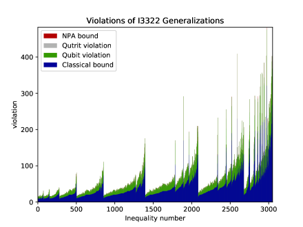
Let us discuss these inqualities. To start with a rough overview, the classical bounds $b_{000}$ of the Bell inequalities range from 8 to 321. Fig. 6 depicts the classical bound for every Bell inequality and how much this bound is exceeded by the quantum states we found as well as the upper bound thereof provided by the NPA hierarchy. We find that all of the inequalities can be violated for qubit states. The inequalities are ordered by simplicity, measured as length of their expression in the above stated notation.

Figure 6: The classical bounds of the inequalities $\sum_{ijk\neq 000}-b_{ijk}\langle A_{i}B_{j}C_{k}\rangle\leq b_{000}$ and their violation by qubits, qutrits and the NPA hierarchy of third level. The Bell inequalities are sorted by the number of terms they incorporate. The orange and blue bars that represent the qutrit violations and NPA bounds can barely be seen because they are mostly hidden behind the bars representing the qubit violations.

Now let us consider some specific Bell inequalities. The largest qutrit-classical ratio $m_{Q}$ is achieved for Bell inequality number 1 as listed in the Supplementary Material, see Appendix C, which reads

$$(110)+(210)-(211)-(220)$$

$$-(222)+2(331)+2(332)\leq 8.$$ (20)

For this inequality, the maximal value attainable with qubits coincides with the upper bound of 16 given by the NPA-hierarchy. It is worth noting that this inequality reduces to Mermin’s inequality if the first two settings of each party are chosen equal. The inequality then is maximally violated for the Greenberger-Horne-Zeilinger state $|GHZ\rangle=(|000\rangle+|111\rangle)/\sqrt{2}$ and the optimal measurement settings for Mermin’s inequality. In fact, this has been already discussed in Ref. Bernards and Gühne (2020) and more details on states and settings can be found there.

We observe the biggest qutrit-qubit ratio $m_{32}$ for Bell inequality number 400, which reads

$$+5(100)+(110)-5(111)+3(200)-3(210)+3(211)$$

$$-2(220)+2(221)-2(300)+(310)+(311)$$

$$+2(322)-(330)$$

$$-(333)\leq 18$$ (21)

For qubits, QM can lead to a violation of $20.928$, whereas for qutrits a maximal violation of $21.157$ can be obtained, which is less than the value $21.238$ obtained using the third level of the NPA-hierarchy.

We find the biggest NPA-qutrit ratio $m_{N}$ for Bell inequality number 1507, which reads

$$8(100)-4(110)+3(111)+4(200)-3(210)$$

$$+2(211)-(220)+2(221)-2(222)-(300)-(310)$$

$$+3(311)+2(320)-(321)+(322)-(331)-(333)\leq 21.$$ (22)

The third level of the NPA hierarchy yields the value $24.079$, which is a significant improvement over the value $26.299$ provided by the second level of the NPA hierarchy. However, with qutrits we could only achieve a violation of $23.603$. With qubits, the violation was even lower at $23.249$.

The largest algebraic-classical ratio $m_{A}$ between the classical bound $12$ and the algebraic bound $86$ is found for Bell inequality number 532. It reads

$$3(100)-(110)-(111)-4(200)+2(210)-(220)$$

$$+(221)+(222)-3(300)+2(310)-(320)+(321)$$

$$-(322)+(331)+(332)\leq 12$$ (23)

All four ratios are listed for the inequalities above in Tab. 1.

Eq.	Number		$m_{Q}$	$m_{32}$	$m_{N}$	$m_{A}$
(20)	1		100.0	0.0	-0.0	250.0
(21)	400		17.54	1.09	0.38	433.33
(22)	1507		12.4	0.61	2.01	514.29
(23)	532		18.69	0.0	0.35	616.67

Table 1: This table shows the relative qutrit violation $m_{Q}$, the qutrit-qubit ratio $m_{32}$, the NPA-qutrit ratio $m_{N}$, and the algebraic-classical ratio $m_{A}$ as well as those generalizations of the I3322 inequality for which one of these margins is the largest. The values of the margins is stated in percent. For example, for inequality number 1, the maximal value of the Bell expression is 16 for qutrit systems, exceeding the classical bound of 8 by 8, yielding $m_{Q}=100\%$.

III.3 Three-party generalizations of the I4422 inequality

When Collins and Gisin discovered the I3322 inequality, they noticed that this Bell inequality is a member of a family of Bell inequalities which they called I$mm$22, where $m\geq 2$. This family contains the CHSH inequality, or I2222, as a special case. Inequalities of this family with more measurement settings generalize inequalities with fewer measurement settings in the following sense: If one substitutes $A_{1}=1$ and $B_{3}=1$ in the I3322 inequality, the inequality effectively reduces to a CHSH inequality. Essentially the same procedure also works for the I4422 inequality Collins and Gisin (2004). In the notation introduced above, it reads

$$2\,(01)+2\,(02)+(03)-(11)-(12)$$

$$- (13)-(14)-(22)-(23)+(24)+(33)\leq 7.$$ (24)

If we substitute $A_{3}=B_{3}=1$, followed by $A_{2}\rightarrow-A_{2}$, $B_{2}\rightarrow-B_{2}$ and $A_{4}\rightarrow-A_{3}$, $B_{4}\rightarrow-B_{3}$, we arrive exactly at the I3322 inequality as stated in Eq. (19).

In contrast to the I3322 inequality we observe a difference between the maximal qubit-violation and the maximal qutrit-violation. For qubits, the largest value we could achieve for the Bell expression is $8$, whereas for qutrits it is $8.15$, which matches the upper bound obtained using the third level of the NPA hierarchy up to numerical precision. Obtaining a value of $8$ is compatible with the above mentioned contraints that will reduce the inequality to the I3322 inequality. This means that the additional measurement setting of I4422 seems to lead to no advantage for achieving a large violation of the inequality, as long as only qubits are concerned. Perhaps surprisingly, the generalizations of I4422 we are going to present do not seem to inherit the feature of being able to discriminate between qubit and qutrit systems by means of their maximal violations.

Before presenting some generalizations of I4422, we should clarify that we did not tackle this problem in full generality. When looking for generalizations of the I3322 inequality to more parties, the only symmetry we demanded was invariance under permutations of parties. Finding generalizations of the I4422 inequality is, however, computationally more involved, which is why we demand a second symmetry in order to make the problem tractable. When choosing a symmetry, one needs to be careful to not impose too strong constraints. For example, a three-party inequality that is invariant under party permutations can never be the generalization of a two party inequality that is not symmetric with respect to the parties. We therefore have to take the symmetries of the inequality we seek to generalize, in our case I4422, into consideration.

Besides being invariant under exchange of the parties $A$ and $B$, I4422 has a second symmetry, namely, if we swap Alice’s first and second setting while simultaneously relabeling the outcomes of Bob’s fourth measurement, then this leaves the inequality invariant. For convenience, we write the symmetries in the following symbolic way:

1. $A\leftrightarrow B$

2. $A_{1}\leftrightarrow A_{2},\quad B_{4}\rightarrow-B_{4}$.

For three-party generalizations of I4422, the following two symmetries seem natural. The first one is

1. $A\leftrightarrow B$

2. $A\leftrightarrow C$

3. $A_{1}\leftrightarrow A_{2}$ , $B_{4}\rightarrow-B_{4}$, $C_{4}\rightarrow-C_{4}$.

However, there exist no non-trivial facet inequalities that generalize I4422 and at the same time meet the above conditions.

We therefore instead look for I4422 generalizations with the following symmetry:

1. $A\leftrightarrow B$

2. $A\leftrightarrow C$

3. $A_{1}\leftrightarrow A_{2}$ , $B_{1}\leftrightarrow B_{2}$, $C_{4}\rightarrow-C_{4}$.

The first two symmetries together establish that the generalizations we are going to find are symmetric under arbitrary permutations of the three parties. The third symmetry resembles the second symmetry of I4422. In total, there are 13 classes of Bell inequalities that generalize I4422 and also exhibit the above symmetries. They are presented in Appendix B.

Figure 7: The classical bounds of the I4422 generalizations and their violation by qubits, qutrits and the NPA hierarchy (second level).

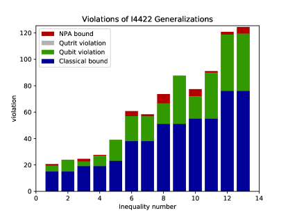
Fig. 7 shows the classical bounds and the violations we found for the 13 inequalities. The more complex scenario of tripartite generalizations of I4422 also comes with the drawback that the third level of the NPA hierarchy is already hard to compute. We therefore only compute the second level of the NPA hierarchy. Tab. 2 shows the relative margins as defined in Eqs. (15 - 18). For all of the inequalities the maximal qubit and qutrit violations we found were the same. However, we cannot be certain that we managed to find the maximal qutrit violation, except from the case of inequality number 5, where the quantum violations attained the upper bound given by the NPA hierarchy up to numerical precision.

Eq.	Number		$m_{Q}$	$m_{32}$	$m_{N}$	$m_{A}$
(32)	1		28.87	0.0	6.81	360.0
(33)	2		59.05	0.0	0.24	413.33
(34)	3		18.39	0.0	9.49	315.79
(35)	4		42.11	0.0	2.18	357.89
(36)	5		69.57	0.0	0.0	434.78
(37)	6		49.83	0.0	6.82	400.0
(38)	7		49.56	0.0	2.75	378.95
(39)	8		30.39	0.0	10.85	341.18
(40)	9		71.33	0.0	0.33	403.92
(41)	10		30.87	0.0	7.56	327.27
(42)	11		63.34	0.0	1.39	385.45
(43)	12		56.21	0.0	1.76	373.68
(44)	13		57.12	0.0	4.26	405.26

Table 2: This table shows the relative qutrit violation $m_{Q}$, the qutrit-qubit ratio $m_{32}$, the NPA-qutrit ratio $m_{N}$, and the algebraic-classical ratio $m_{A}$ for every generalization of I4422 that satisfies the symmetry described in the text. The values of the ratios are expressed in percent. Numbers refers to the number under which the corresponding inequality is listed in the Appendix B.

III.4 Three-party hybrid CHSH-I3322 generalizations

To show that also hybrid scenarios can be studied, we find all 476 three-party facet Bell inequalities with the following properties: Alice and Bob have three measurement settings each and Charlie has only two. Also, there are deterministic assignments to the outcomes of Alice’s measurements, such that the inequality effectively reduces to the CHSH inequality

$$\langle{A_{1}B_{1}}\rangle+\langle{A_{1}B_{2}}\rangle+\langle{A_{2}B_{1}}\rangle-\langle{A_{2}B_{2}}\rangle\leq 2.$$ (25)

Further, there are deterministic assignments to the outcomes of Charlie’s measurements, such that the inequality reduces to the I3322 inequality. Lastly, we require the inequality to be symmetric under exchange of Alice and Bob. These conditions lead to 476 inequalities, these are given in the Supplementary Material, see Appendix C.

As one can see in Fig. 8 all of the Bell inequalities are violated in quantum mechanics. The strongest violation by qutrit states is achieved for inequality $47$. It reads

$$\langle C_{1}\rangle+\langle C_{2}\rangle+\langle B_{1}\rangle$$

$$-\langle B_{1}C_{2}\rangle-\langle B_{2}\rangle+\langle B_{2}C_{1}\rangle+\langle A_{1}\rangle$$

$$-\langle A_{1}C_{2}\rangle+2\langle A_{1}B_{1}C_{2}\rangle+\langle A_{1}B_{2}\rangle-\langle A_{1}B_{2}C_{1}\rangle$$

$$-\langle A_{1}B_{3}C_{1}\rangle-\langle A_{1}B_{3}C_{2}\rangle-\langle A_{2}\rangle+\langle A_{2}C_{1}\rangle$$

$$+\langle A_{2}B_{1}\rangle-\langle A_{2}B_{1}C_{1}\rangle-\langle A_{2}B_{2}\rangle+2\langle A_{2}B_{2}C_{1}\rangle$$

$$-\langle A_{2}B_{2}C_{2}\rangle+\langle A_{2}B_{3}\rangle-\langle A_{2}B_{3}C_{2}\rangle-\langle A_{3}B_{1}C_{1}\rangle$$

$$-\langle A_{3}B_{1}C_{2}\rangle+\langle A_{3}B_{2}\rangle-\langle A_{3}B_{2}C_{2}\rangle-\langle A_{3}B_{3}\rangle$$

$$-\langle A_{3}B_{3}C_{1}\rangle\leq 6$$ (26)

Figure 8: The classical bounds of the inequalities $\sum_{ijk\neq 000}-b_{ijk}\langle A_{i}B_{j}C_{k}\rangle\leq b_{000}$ and their violation by qubits, qutrits and the NPA hierarchy of third level. See text for further details.

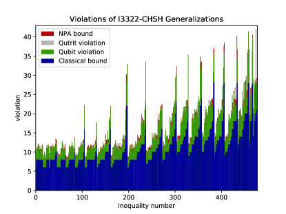
We find the largest NPA-qutrit ratio $m_{N}$ for Bell inequality number 314. It reads

$$5\langle C_{1}\rangle+\langle C_{2}\rangle+2\langle B_{1}\rangle-2\langle B_{1}C_{1}\rangle$$

$$-2\langle B_{2}\rangle+2\langle B_{2}C_{1}\rangle+\langle B_{3}C_{1}\rangle+\langle B_{3}C_{2}\rangle$$

$$+2\langle A_{1}\rangle-2\langle A_{1}C_{1}\rangle+2\langle A_{1}B_{1}C_{1}\rangle-2\langle A_{1}B_{1}C_{2}\rangle$$

$$+\langle A_{1}B_{2}\rangle-2\langle A_{1}B_{2}C_{1}\rangle+\langle A_{1}B_{2}C_{2}\rangle$$

$$+\langle A_{1}B_{3}\rangle-2\langle A_{1}B_{3}C_{1}\rangle+\langle A_{1}B_{3}C_{2}\rangle-2\langle A_{2}\rangle$$

$$+2\langle A_{2}C_{1}\rangle+\langle A_{2}B_{1}\rangle-2\langle A_{2}B_{1}C_{1}\rangle+\langle A_{2}B_{1}C_{2}\rangle$$

$$-2\langle A_{2}B_{2}\rangle+3\langle A_{2}B_{2}C_{1}\rangle+\langle A_{2}B_{2}C_{2}\rangle+\langle A_{2}B_{3}\rangle$$

$$-3\langle A_{2}B_{3}C_{1}\rangle+\langle A_{3}C_{1}\rangle+\langle A_{3}C_{2}\rangle+\langle A_{3}B_{1}\rangle$$

$$-2\langle A_{3}B_{1}C_{1}\rangle+\langle A_{3}B_{1}C_{2}\rangle+\langle A_{3}B_{2}\rangle$$

$$-3\langle A_{3}B_{2}C_{1}\rangle-2\langle A_{3}B_{3}C_{1}\rangle-2\langle A_{3}B_{3}C_{2}\rangle\leq 12.$$ (27)

We achieve the same violation for qubit and qutrit systems at $16.339$. The third level of the NPA hierarchy yields $16.488$, improving the upper bound of $17.870$ from the second level NPA hierarchy significantly. Because the qubit and qutrit violations are the same, one may conjecture that the upper bound for the quantum mechanical violation provided by the NPA hierarchy is not tight for the third level.

We observe the biggest gap between qubits and qutrits for Bell inequality number 1. It reads

$$2\langle B_{1}\rangle-2\langle B_{2}\rangle+2\langle A_{1}\rangle-\langle A_{1}B_{1}\rangle$$

$$+\langle A_{1}B_{1}C_{1}\rangle+\langle A_{1}B_{2}\rangle-\langle A_{1}B_{2}C_{1}\rangle+2\langle A_{1}B_{3}C_{2}\rangle$$

$$-2\langle A_{2}\rangle+\langle A_{2}B_{1}\rangle-\langle A_{2}B_{1}C_{1}\rangle-\langle A_{2}B_{2}\rangle$$

$$+\langle A_{2}B_{2}C_{1}\rangle+2\langle A_{2}B_{3}C_{2}\rangle+2\langle A_{3}B_{1}C_{2}\rangle+2\langle A_{3}B_{2}C_{2}\rangle$$

$$\leq 8$$ (28)

For this inequality we find a value of $10.000$ for qubits, whereas the violation of $10.286$ that we find for qutrits coincides with the value of the third level of the NPA hierarchy up to numerical precision.

Lastly, the biggest gap between the classical and the algebraic bound occurs for inequality $198$, which reads

$$3\langle C_{1}\rangle+\langle C_{2}\rangle+2\langle B_{1}\rangle$$

$$-\langle B_{1}C_{1}\rangle-\langle B_{1}C_{2}\rangle-\langle B_{2}\rangle+2\langle B_{2}C_{1}\rangle$$

$$+\langle B_{2}C_{2}\rangle+\langle B_{3}\rangle-\langle B_{3}C_{2}\rangle+2\langle A_{1}\rangle$$

$$-\langle A_{1}C_{1}\rangle-\langle A_{1}C_{2}\rangle-\langle A_{1}B_{1}\rangle+\langle A_{1}B_{1}C_{1}\rangle$$

$$+\langle A_{1}B_{2}\rangle-\langle A_{1}B_{2}C_{1}\rangle-\langle A_{1}B_{3}C_{1}\rangle+\langle A_{1}B_{3}C_{2}\rangle$$

$$-\langle A_{2}\rangle+2\langle A_{2}C_{1}\rangle+\langle A_{2}C_{2}\rangle+\langle A_{2}B_{1}\rangle$$

$$-\langle A_{2}B_{1}C_{1}\rangle-\langle A_{2}B_{2}\rangle-\langle A_{2}B_{2}C_{2}\rangle+\langle A_{2}B_{3}\rangle$$

$$-\langle A_{2}B_{3}C_{1}\rangle+\langle A_{3}\rangle-\langle A_{3}C_{2}\rangle-\langle A_{3}B_{1}C_{1}\rangle$$

$$+\langle A_{3}B_{1}C_{2}\rangle+\langle A_{3}B_{2}\rangle-\langle A_{3}B_{2}C_{1}\rangle\leq 6.$$ (29)

Compared to the classical bound of $6$, the algebraic bound is almost seven times as large at $40$. The numerical results are summarized in Tab. 3.

Eq.	Number		$m_{Q}$	$m_{32}$	$m_{N}$	$m_{A}$
(26)	47		69.23	0.0	0.0	400.0
(28)	1		28.57	2.86	0.0	200.0
(27)	314		36.16	0.0	0.91	433.33
(29)	198		39.71	0.0	0.0	566.67

Table 3: This table shows the relative qutrit violation $m_{Q}$, the qutrit-qubit ratio $m_{32}$, the NPA-qutrit ratio $m_{N}$, and the algebraic-classical ratio $m_{A}$ as well as those hybrid generalizations of the I3322 and the CHSH inequality for which one of these margins is the largest. The values of the ratios is stated in percent.

III.5 Four-party generalizations of a Guess-Your-Neighbors-Input inequality

In this section we present generalizations of a guess your neighbors input (GYNI) Bell inequality. GYNI inequalities give a classical upper bound for the winning probability of the nonlocal game that goes by the same name. The game is played with $N$ parties that are arranged in a ring and collaboratively play against the instructor. The instructor will supply every participant $i$ with an input bit $x_{i}$ and each participant then has to guess the input of his left neighbor. The game is won if the output $a_{i}$ of every player output matches the input $x_{i+1}$ of their left neighbor. In order to achieve this goal, the players may agree on a strategy before the game and they are also provided with the probability distribution $q(\bm{x})$ according to which the instructor chooses the inputs. In the quantum version of the game, the parties additionally possess a part of a shared quantum state. During the game, no communication is permitted. A GYNI inequality is an inequality of the form

$$\sum_{\bm{x}}q(\bm{x})P(a_{i}=x_{i+1}\forall i|\bm{x})\leq\omega_{c},$$ (30)

whereby the left-hand-side expresses the average winning probability, which is bounded by the average winning probability of the best classical strategy $\omega_{c}$. Notably, Almeida et al Almeida et al. (2010) showed that GYNI Bell inequalities are never violated by quantum theory and discovered that a facet defining Bell-inequality previously found by Śliwa is a GYNI inequality. This inequality, written in observable notation, reads

$$\langle{A_{1}B_{1}}\rangle+\langle{A_{2}B_{1}}\rangle+\langle{A_{1}B_{2}}\rangle+\langle{A_{2}B_{2}}\rangle$$

$$+\langle{A_{1}C_{1}}\rangle-\langle{A_{2}C_{1}}\rangle+\langle{B_{1}C_{1}}\rangle+\langle{A_{1}B_{1}C_{1}}\rangle$$

$$-\langle{B_{2}C_{1}}\rangle-\langle{A_{2}B_{2}C_{1}}\rangle+\langle{A_{1}C_{2}}\rangle-\langle{A_{2}C_{2}}\rangle-\langle{B_{1}C_{2}}\rangle$$

$$+\langle{A_{2}B_{1}C_{2}}\rangle+\langle{B_{2}C_{2}}\rangle-\langle{A_{1}B_{2}C_{2}}\rangle\leq 4$$ (31)

and is listed as inequality number $10$ in the paper by Śliwa Śliwa (2003). Here we present its generalizations. The inequality has the following symmetries:

1. $A_{1}\leftrightarrow A_{2}$, $B_{1}\leftrightarrow B_{2}$, $C_{1}\rightarrow-C_{1}$, $C_{2}\rightarrow-C_{2}$

2. $A_{1}\leftrightarrow A_{2}$, $C_{1}\leftrightarrow C_{2}$, $A_{i}\rightarrow-A_{i}\forall i$, $B_{i}\rightarrow-B_{i}\forall i$.

Figure 9: The classical bounds of the inequalities $\sum_{ijkl\neq 0000}-b_{ijkl}\langle A_{i}B_{j}C_{k}D_{l}\rangle\leq b_{0000}$ and their violation by qubits, qutrits and the NPA hierarchy of third level.

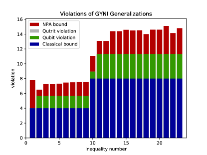
We demand exactly the same symmetries for the generalization of the above inequality. We find $23$ four-partite inequalities, the detailed expressions are given in the Supplementary Material, see Appendix C. The first one is not a real four-partite Bell inequality, since it only includes a single measurement setting on the fourth party. In fact, it is of the form $B(1+D_{1})\leq 4(1+D_{1})$, where $B$ is the left-hand-side of Eq. (31) after $C_{1}$ and $C_{2}$ have been swapped and all outcomes of Bob have been relabeled. All the other inequalities are violated in quantum theory. Hence, none of the generalizations shares the characteristic feature of the GYNI inequality. Fig. 9 shows a plot with all classical bounds and their violations for all 23 inequalities.

IV Conclusion

We discussed the cone-projection technique as a method to find facet Bell inequalities with normal vectors that obey linear constraints. We further introduced the concept of a generalization of a Bell inequality to more parties. The property of being a generalization of a specific Bell inequality can be formulated as a linear constraint on its normal vector. Using the cone-projection technique, we were able to find 3050 classes of generalizations of the I3322 inequality, 476 classes of Bell inequalities that simultaneously generalize the CHSH inequality as well as the I3322 inequality, 13 classes of Bell inequalities that generalize the I4422 inequality and 23 classes of Bell inequalities that generalize the Guess-Your-Neighbors-Input inequality first found in Śliwa (2003). For all inequalities, we applied an extensive numerical analysis, providing upper bounds to their quantum violations both for qubit and qutrit systems as well as upper bounds using the NPA hierarchy.

For future research, there are several open problems. First, it would be desirable to study some of the Bell inequalities presented here in more detail. For instance, the question arises whether they can be connected to some distributed information processing task. In addition, one may study the viability of an experimental test of these inequalities. Second, it is very interesting to study the cone-projection technique also for other scenarios, such as Bell inequalities that detect genuine multi-partite nonlocality or contextuality inequalities.

Appendix A Details on finding lower bounds for qubit and qutrit violations

We provide lower bounds for the violations of the Bell inequalities achievable with qubits and qutrits, respectively. These lower bounds are violations achieved by specific states and measurements.

Finding good lower bounds therefore involves two optimizations: One optimization over the possible states and another optimization over the measurement settings. The objective – that is the expectation value of the Bell operator for the given state – is however not linear, if we optimize over all measurements at once. We therefore break the optimization over the measurement settings down further to optimizing over them party by party, thereby rendering the objective linear. We represent each measurement by a positive operator-valued measure (POVM). Such a optimization problem that features an objective that is linear in its arguments which are positive-semidefinite operators is called a semidefinite program (SDP) and can be solved efficiently. Likewise, the optimization over the state-space while keeping the measurement settings constant is also an SDP.

This prompts a seesaw-algorithm: After initializing the measurement settings to (pseudo-)random values, we alternate between updating the quantum state and updating the measurement settings one party at a time while keeping the quantum state constant. In this way, the value of the objective is guaranteed to increase monotonically and will eventually converge, if the objective is bounded. However, it oftentimes only converges to a local minimum. This is a problem we cannot avoid, but we can aim for a rather good local optimum by running the seesaw-algorithm many times, starting at a different initial state every time. To save computational resources, we do not wait until the objective values reach high precision. Instead, we stop after a few iterations, select the most promising instance of the optimization and only continue the seesaw-algorithm for this selected instance until the improvements of the objective value fall below some threshold.

Appendix B I4422 generalizations

We find 13 classes of Bell inequalities that are symmetric under party permutations, generalize I4422 and further exhibit the symmetry $A_{1}\leftrightarrow A_{2},B_{1}\leftrightarrow B_{2},C_{4}\rightarrow-C_{4}$. In the notation for symmetric Bell inequalities that we introduced in the main text, they read

$$-(100)-2(110)-(200)-2(210)-2(220)+(300)-(310)$$

$$\qquad\quad-(320)+(330)+(331)+(332)-3(333)+2(441)-2(442) \leq 15\qquad\quad$$ (32)

$$-(100)-2(110)-(111)-(200)-2(210)+(211)-2(220)-(221)+(222)$$

$$\qquad\quad+(300)-(310)-(320)+(330)+(331)+(332)-3(333)+2(441)-2(442) \leq 15\qquad\quad$$ (33)

$$-2(100)-2(110)-2(200)-2(210)-2(220)-(300)-2(310)-2(320)$$

$$\qquad\quad+(330)-(333)+2(441)-2(442) \leq 19\qquad\quad$$ (34)

$$-2(100)-2(110)-(111)-2(200)-2(210)+(211)-2(220)-(221)$$

$$\qquad\quad+(222)-(300)-2(310)-2(320)+(330)-(333)+2(441)-2(442) \leq 19\qquad\quad$$ (35)

$$+3(100)-3(110)+2(111)+3(200)-3(210)-3(220)+2(221)+(300)-(310)$$

$$\qquad\quad+(311)-(320)+(321)+(322)+(330)-(331)-(332)+(333)-4(441)+4(442) \leq 23\qquad\quad$$ (36)

$$+3(100)+(110)-3(111)+3(200)+(210)+(211)+(220)-3(221)+(222)+4(300)$$

$$\qquad\quad+3(310)-3(311)+3(320)-3(321)-3(322)-6(330)-(331)-(332)+12(333)+4(441)-4(442) \leq 38\qquad\quad$$ (37)

$$+3(100)+(110)-(111)+3(200)+(210)-(211)+(220)-(221)-(222)+4(300)+3(310)-3(311)$$

$$\qquad\quad+3(320)-3(321)-3(322)-6(330)-(331)-(332)+12(333)+4(441)-4(442) \leq 38\qquad\quad$$ (38)

$$+2(100)-5(110)+2(200)-5(210)-5(220)+(300)-4(310)+3(311)-4(320)$$

$$\qquad\quad+3(321)+3(322)+(330)-2(331)-2(332)-3(333)-8(441)+8(442) \leq 51\qquad\quad$$ (39)

$$+2(100)-5(110)-4(111)+2(200)-5(210)+4(211)-5(220)-4(221)+4(222)+(300)$$

$$\qquad\quad-4(310)+3(311)-4(320)+3(321)+3(322)+(330)-2(331)-2(332)-3(333)+8(441)-8(442) \leq 51\qquad\quad$$ (40)

$$+(100)-5(110)+(200)-5(210)-5(220)-(300)-5(310)+3(311)-5(320)$$

$$\qquad\quad+3(321)+3(322)+(330)-3(331)-3(332)-(333)-8(441)+8(442) \leq 55\qquad\quad$$ (41)

$$+(100)-5(110)-4(111)+(200)-5(210)+4(211)-5(220)-4(221)+4(222)-(300)$$

$$\qquad\quad-5(310)+3(311)-5(320)+3(321)+3(322)+(330)-3(331)-3(332)-(333)+8(441)-8(442) \leq 55\qquad\quad$$ (42)

$$+7(100)+(110)-(111)+7(200)+(210)-(211)+(220)-(221)-(222)+6(300)+7(310)-7(311)$$

$$\qquad\quad+7(320)-7(321)-7(322)-12(330)-(331)-(332)+22(333)-8(441)+8(442) \leq 76\qquad\quad$$ (43)

$$+7(100)+(110)-5(111)+7(200)+(210)+3(211)+(220)-5(221)+3(222)+6(300)+7(310)-7(311)$$

$$\qquad\quad+7(320)-7(321)-7(322)-12(330)-(331)-(332)+22(333)+8(441)-8(442) \leq 76.\qquad\quad$$ (44)

Appendix C Content of the online material

The further online material (included in the source files of this arxiv submission) contains the generalizations of the I3322 inequality, the I4422 inequality, the Guess-Your-Neighbors-Input inequality (Eq. (LABEL:eq:gyni)), and the hybrid I3322-CHSH Bell inequalities. For convenience, the online material includes four files, one for each class of Bell inequalities:

• i3322gensquant.txt This file contains the generalizations of the I3322 inequality.

• i4422gensquant.txt This file contains the generalizations of the I4422 inequality.

• hybridgensquant.txt This file contains the hybrid I3322-CHSH inequalities.

• gynigensquant.txt This file contains the generalizations of the GYNI inequality in Eq. (31).

Each file lists the Bell inequalities together with their respective algebraic bounds as well as the bounds obtained from the second level of the NPA-hierarchy and, with the exception of I4422 generalizations, also from the third level of the NPA-hierarchy. Additionally, we provide lower bounds on the qubit violations and qutrit violations as well as the corresponding qubit state and qubit settings that lead to the listed qubit violation.

References

- Brunner et al. (2014) N. Brunner, D. Cavalcanti, S. Pironio, V. Scarani, and S. Wehner, Rev. Mod. Phys. 86, 419 (2014).
- Scarani (2019) V. Scarani, Bell Nonlocality (Oxford University Press, 2019).
- Shalm et al. (2015) L. K. Shalm, E. Meyer-Scott, B. G. Christensen, P. Bierhorst, M. A. Wayne, M. J. Stevens, T. Gerrits, S. Glancy, D. R. Hamel, M. S. Allman, K. J. Coakley, S. D. Dyer, C. Hodge, A. E. Lita, V. B. Verma, C. Lambrocco, E. Tortorici, A. L. Migdall, Y. Zhang, D. R. Kumor, W. H. Farr, F. Marsili, M. D. Shaw, J. A. Stern, C. Abellán, W. Amaya, V. Pruneri, T. Jennewein, M. W. Mitchell, P. G. Kwiat, J. C. Bienfang, R. P. Mirin, E. Knill, and S. W. Nam, Phys. Rev. Lett. 115, 250402 (2015).
- Hensen et al. (2015) B. Hensen, H. Bernien, A. Dréau, A. Reiserer, N. Kalb, M. Blok, J. Ruitenberg, R. Vermeulen, R. Schouten, C. Abellan, W. Amaya, V. Pruneri, M. Mitchell, M. Markham, D. Twitchen, D. Elkouss, S. Wehner, T. Taminiau, and R. Hanson, Nature 526, 682 (2015).
- Giustina et al. (2015) M. Giustina, M. A. M. Versteegh, S. Wengerowsky, J. Handsteiner, A. Hochrainer, K. Phelan, F. Steinlechner, J. Kofler, J.-A. Larsson, C. Abellán, W. Amaya, V. Pruneri, M. W. Mitchell, J. Beyer, T. Gerrits, A. E. Lita, L. K. Shalm, S. W. Nam, T. Scheidl, R. Ursin, B. Wittmann, and A. Zeilinger, Phys. Rev. Lett. 115, 250401 (2015).
- Rosenfeld et al. (2017) W. Rosenfeld, D. Burchardt, R. Garthoff, K. Redeker, N. Ortegel, M. Rau, and H. Weinfurter, Phys. Rev. Lett. 119, 010402 (2017).
- Šupić and Bowles (2020) I. Šupić and J. Bowles, Quantum 4, 337 (2020).
- Holz et al. (2019) T. Holz, H. Kampermann, and D. Bruß, “A genuine multipartite Bell inequality for device-independent conference key agreement,” (2019), arXiv:1910.11360 [quant-ph] .
- Almeida et al. (2010) M. L. Almeida, J.-D. Bancal, N. Brunner, A. Acín, N. Gisin, and S. Pironio, Phys. Rev. Lett. 104, 230404 (2010).
- Peres (1999) A. Peres, Foundations of Physics 29, 589 (1999).
- Pitowsky (1991) I. Pitowsky, Mathematical Programming 50, 395 (1991).
- Clauser et al. (1969) J. F. Clauser, M. A. Horne, A. Shimony, and R. A. Holt, Phys. Rev. Lett. 23, 880 (1969).
- Clauser et al. (1970) J. F. Clauser, M. A. Horne, A. Shimony, and R. A. Holt, Phys. Rev. Lett. 24, 549 (1970).
- Froissart (1981) M. Froissart, Il Nuovo Cimento B (1971-1996) 64, 241 (1981).
- Śliwa (2003) C. Śliwa, Phys. Lett. A 317, 165 (2003).
- Collins and Gisin (2004) D. Collins and N. Gisin, J. Phys. A: Math. Gen. 37, 1775 (2004).
- Bernards and Gühne (2020) F. Bernards and O. Gühne, Phys. Rev. Lett. 125, 200401 (2020).
- Ziegler (1995) G. M. Ziegler, Lectures on Polytopes: Updated Seventh Printing of the First Edition, Graduate Texts in Mathematics 152 (Springer-Verlag New York, 1995).
- Pironio (2005) S. Pironio, Journal of Mathematical Physics 46, 062112 (2005).
- Navascués et al. (2007) M. Navascués, S. Pironio, and A. Acín, Phys. Rev. Lett. 98, 010401 (2007).
- Wittek (2015) P. Wittek, ACM Trans. Math. Softw. 41 (2015), 10.1145/2699464.
- Pál and Vértesi (2010) K. F. Pál and T. Vértesi, Phys. Rev. A 82, 022116 (2010).