Accurate and Efficient Modeling of the Transverse Mode Instability in High Energy Laser Amplifiers

Abstract

We study the transverse mode instability (TMI) in the limit where a single higher-order mode (HOM) is present. We demonstrate that when the beat length between the fundamental mode and the HOM is small compared to the length scales on which the pump amplitude and the optical mode amplitudes vary, TMI is a three-wave mixing process in which the two optical modes beat with the phase-matched component of the index of refraction that is induced by the thermal grating. This limit is the usual limit in applications, and in this limit TMI is identified as a stimulated thermal Rayleigh scattering (STRS) process. We demonstrate that a phase-matched model that is based on the three-wave mixing equations can have a large computational advantage over current coupled mode methods that must use longitudinal step sizes that are small compared to the beat length.

1 Introduction

Ytterbium-doped fiber amplifiers that produce kilowatt output powers have been developed in the past decade [1, 2, 3, 4, 5, 6, 7]. However, the thermal or transverse mode instability (TMI) has become a major barrier to achieving even higher output powers [8, 9, 10]. Despite almost a decade of work since the original observation of TMI in fiber amplifiers by Jauregui et al. [11] and Eidam et al. [12], it still remains only partially understood, and computationally-efficient methods that are sufficiently accurate for amplifier design have been lacking. It was recognized early by Smith and Smith [13] that the instability could be explained by a thermal grating that is induced by the beating of the fundamental mode of the optical fiber with a higher-order mode at a slightly lower frequency and the quantum defect heating that ensues.

Subsequent work by Jauregui et al. [14], Dong [15], and Smith and Smith [16] identified the instability as a stimulated thermal Rayleigh scattering (STRS) process. In particular, Dong [15] developed a three-wave mixing model that is analogous to models of the Brillouin instability due to stimulated Brillouin scattering (SBS). This identification has remained somewhat controversial, although Kong et al. [17] directly observed the STRS process in a fiber amplifier. Ward et al. [18] and Naderi et al. [19] developed a model of TMI based on a coupled mode method that makes no reference to three-wave interactions. The complexity of TMI has obscured its identification as an STRS-driven, three-wave process. The conditions that are required to treat TMI as a three-wave instability have not been elucidated.

In this work, we demonstrate that the key requirement is that the beat length $L_{\rm B}=2\pi$/$\Delta\beta$ must be small compared to any other longitudinal scale lengths, where $\Delta\beta$ is the difference between the wavenumber of the fundamental mode and any higher-order modes (HOMs) at the same frequency. This condition usually applies in practice. In this limit, we derive the three-wave equations that govern TMI. Terms that are not phase-matched are neglected. This approach is similar to Dong’s approach [15], but is more general.

We further demonstrate that this approach has a large computational advantage. Approaches that use the coupled mode method, like the approach of Naderi et al. [19], must use longitudinal steps in their computations that are small compared to the beat length. As a result, Naderi et al. [19] limited their study to a high-gain amplifier with a length of 1.6 m, which is substantially shorter than typical ytterbium-doped fiber amplifiers. Approaches that use the finite-element method to calculate the optical mode profile on each longitudinal step like that of Ward [20] must take steps that are small compared to the optical wavelength and typically require large computational resources. Our approach is only limited by the longitudinal scale lengths over which the amplitudes of the optical modes, the thermal mode, and the pump mode change. These lengths are typically far larger than the beat length. For the examples that we consider in this paper, which correspond to realistic Yb³⁺-doped fiber amplifiers, the computational speedup is more than a factor of 100.

2 Theoretical Model

We may write the index of refraction as $n({\bf r}_{\perp},z,t)=n_{0}({\bf r}_{\perp})+\Delta n({\bf r}_{\perp},z,t)$, where $n_{0}({\bf r}_{\perp})$ is the unperturbed index of refraction, and we set $\Delta n\ll n_{0}$, which is always the case ($\Delta n/n_{0}\sim 10^{-5}$). We will use the slowly varying envelope approximation, which is an excellent approximation in this system due to the large discrepancy between the wavelength and the next-smallest scale, which is the intermodal beat length $L_{\rm B}$. We will also assume that time derivatives of the index of refraction can be ignored when calculating the inter-modal coupling. That is again an excellent approximation, given the large disparity between the light period and the time scale on which either the gain changes (microseconds) or the temperature changes (milliseconds). We assume as well that the only coupling is between modes that are propagating in the forward direction. We start with the expression from coupled mode theory for two coupled modes [21, 22],

$$\begin{split}\frac{dA_{0}}{dz}=\frac{i\omega^{2}}{\beta c^{2}}\int d^{2}{\bf r}_{\perp}n_{0}\Delta n\left[|\mathbfcal{E}_{0}|^{2}A_{0}+\mathbfcal{E}_{0}^{*}\cdot\mathbfcal{E}_{1}\exp(-i\Delta\beta z)A_{1}\right],\\ \frac{dA_{1}}{dz}=\frac{i\omega^{2}}{\beta c^{2}}\int d^{2}{\bf r}_{\perp}n_{0}\Delta n\left[|\mathbfcal{E}_{1}|^{2}A_{1}+\mathbfcal{E}_{1}^{*}\cdot\mathbfcal{E}_{0}\exp(i\Delta\beta z)A_{0}\right],\end{split}$$ (1)

where $\mathbfcal{E}_{0}$ and $\mathbfcal{E}_{1}$ are the normalized transverse mode profiles for the fundamental mode and the HOM, while $A_{0}$ and $A_{1}$ are the corresponding amplitudes. We have set $\beta\equiv\beta_{0}\approx\beta_{1}$ since $\Delta\beta=\beta_{0}-\beta_{1}\ll\beta_{0,1}$. Equation (1) is valid when only a single HOM is present or when the amplitudes of the other HOMs are small compared to $A_{0}$ and $A_{1}$.

To solve Eq. (1) at any point in time $t$, we must find $\Delta n({\bf r}_{\perp},z,t)$. Due to the factors $\exp(\pm i\Delta\beta z)$ that appear in Eq. (1), it is necessary to determine $\Delta n({\bf r}_{\perp},z,t)$ with a computational resolution $\Delta z$ that is small compared to the beat length $L_{\rm B}=2\pi/\Delta\beta$ even though the field amplitudes vary slowly compared to this length. Since we must determine the transverse dependence of $\Delta n$ as well, this constraint is computationally demanding. We can bypass this difficulty by replacing the field $\Delta n({\bf r}_{\perp},z,t)$ with three fields $n_{0}({\bf r}_{\perp},z,t)$, $n_{+}({\bf r}_{\perp},z,t)$, and $n_{-}({\bf r}_{\perp},z,t)$, which are defined so that

$$\Delta n=\Delta n_{0}+\frac{1}{2}[\Delta n_{+}\exp(i\Delta\beta z)+\Delta n_{-}\exp(-i\Delta\beta z),$$ (2)

and all three fields vary slowly compared to the beat length $L_{\rm B}$. When we substitute Eq. (2) into Eq. (1) and keep only the phase-matched terms, we obtain

$$\begin{split}\frac{dA_{0}}{dz}=\frac{i\omega^{2}}{\beta c^{2}}\int d^{2}{\bf r}_{\perp}n_{0}\left[|\mathbfcal{E}_{0}|^{2}\Delta n_{0}A_{0}+\frac{1}{2}\mathbfcal{E}_{0}^{*}\cdot\mathbfcal{E}_{1}\Delta n_{+}A_{1}\right],\\ \frac{dA_{1}}{dz}=\frac{i\omega^{2}}{\beta c^{2}}\int d^{2}{\bf r}_{\perp}n_{0}\left[|\mathbfcal{E}_{1}|^{2}\Delta n_{0}A_{1}+\frac{1}{2}\mathbfcal{E}_{1}^{*}\cdot\mathbfcal{E}_{0}\Delta n_{-}A_{0}\right].\end{split}$$ (3)

The terms that are not phase-matched are rapidly oscillating and do not contribute significantly to the integrals. All terms in Eq. (3) vary slowly in $z$. It then becomes possible to integrate Eq. (3) with no loss of accuracy while using a resolution in $z$ that is far larger than is necessary with Eq. (1).

The form of Eq. (3) makes clear that in the limit where Eq. (3) is valid, TMI is effectively a three-wave process in which two optical fields combine with a density field. The condition for Eq. (3) to be valid is that all terms must vary slowly compared to the beat length. This condition is almost always met in practice. Since the density field is thermally driven, this process is a stimulated Rayleigh scattering process. We discuss this identification in more detail in the Appendix.

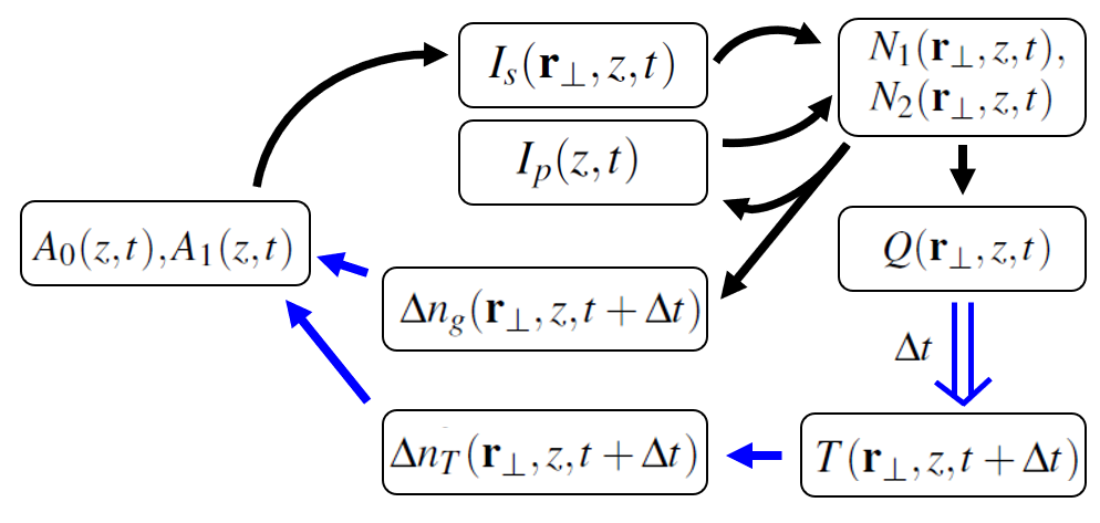
Figure 1: Schematic flow diagram of the computational procedure. The time step occurs when $T(t+\Delta t)$ is calculated using $Q(t)$.

The procedure that we use to obtain $\Delta n_{0}$, $\Delta n_{+}$, and $\Delta n_{-}$ in terms of the field and as a function of time is analogous to the procedure that is used by Naderi et al. [19] that is illustrated in Fig. 1.

We begin by writing the signal intensity $I_{s}({\bf r}_{\perp},z,t)$ as

$$I_{s}({\bf r}_{\perp},z,t)=I_{s0}+\frac{1}{2}\left[I_{s+}\exp(i\Delta\beta z)+I_{s-}\exp(-i\Delta\beta z)\right],$$ (4)

where

$$I_{s0}=\frac{\beta}{2\mu_{0}\omega}\left(|\mathbfcal{E}_{0}|^{2}|A_{0}|^{2}+|\mathbfcal{E}_{1}|^{2}|A_{1}|^{2}\right),\qquad I_{s+}=I_{s-}^{*}=\frac{\beta}{\mu_{0}\omega}\mathbfcal{E}_{1}^{*}\cdot\mathbfcal{E}_{0}A_{1}^{*}A_{0},$$ (5)

all vary slowly compared to $L_{B}$. The behavior of a Yb-doped fiber amplifier is accurately described as a two-level system at realistic power levels [2]. Given $I_{s}({\bf r}_{\perp},z,t)$ and the pump intensity $I_{p}(z,t)$, we next compute the upper state density $N_{2}({\bf r}_{\perp},z,t)$ of the Yb ions, which is given by

$$N_{2}={\sigma_{p}^{\rm(a)}(I_{p}/\hbar\omega_{p})+\sigma_{s}^{\rm(a)}(I_{s}/\hbar\omega)\over\left[\sigma_{p}^{\rm(a)}+\sigma_{p}^{\rm(e)}\right](I_{p}/\hbar\omega_{p})+\left[\sigma_{s}^{\rm(a)}+\sigma_{s}^{\rm(e)}\right](I_{s}/\hbar\omega)+1/\tau}N_{0},$$ (6)

where $\omega$ and $\omega_{p}$ are the signal and pump angular frequencies, respectively, $\tau$ is the spontaneous decay time of the upper level, $N_{0}$ is total density of Yb ions, and $\sigma_{p}^{\rm(a)}$, $\sigma_{p}^{\rm(e)}$, $\sigma_{s}^{\rm(a)}$, and $\sigma_{s}^{\rm(e)}$ are the absorption and emission cross-sections at the pump and signal frequencies. Because $I_{s}$ appears in both the numerator and denominator of Eq. (6), the density $N_{2}$ will have higher harmonics that are proportional to $\exp(\pm im\Delta\beta)$ with $m>1$. We will truncate this expression since the harmonics with $m>1$ are not phase-matched. Explicitly, we find that Eq. (6) has the form

$$N_{2}={A+B\cos\theta\over C+D\cos\theta}N_{0},$$ (7)

where $\theta=\Delta\beta z+\phi$ and $\phi=\angle(A_{1}^{*}A_{0}\mathbfcal{E}_{1}^{*}\cdot\mathbfcal{E}_{0})$. We have

$$\begin{split}\hskip 56.9055ptA=\sigma_{p}^{\rm(a)}{I_{p}\over\hbar\omega_{p}}+\sigma_{s}^{\rm(a)}{I_{s0}\over\hbar\omega},\qquad B=\sigma_{s}^{\rm(a)}{|I_{s+}|\over\hbar\omega},\\ C=\left[\sigma_{p}^{\rm(a)}+\sigma_{p}^{\rm(e)}\right]{I_{p}\over\hbar\omega_{p}}+\left[\sigma_{s}^{\rm(a)}+\sigma_{s}^{\rm(e)}\right]{I_{s0}\over\hbar\omega}+{1\over\tau},\\ \qquad D=\left[\sigma_{s}^{\rm(a)}+\sigma_{s}^{\rm(e)}\right]{|I_{s+}|\over\hbar\omega}.\end{split}$$ (8)

We note that $D<C$ and $B<C$ is a consequence of $I_{s+}<I_{s0}$, which in turn follows from the Cauchy-Schwartz inequality. We now write

$$N_{2}\simeq N_{20}+{1\over 2}\left[N_{2+}\exp(i\Delta\beta z)+N_{2-}\exp(-i\Delta\beta z)\right],$$ (9)

where

$$\begin{split}N_{20}={A\over C}{1\over r}\left(1-{BD\over AC}{1\over 1+r}\right)N_{0},\\ N_{2+}=N_{2-}^{*}={A\over C}{2\over r(1+r)}\left({B\over A}-{D\over C}\right)N_{0}\exp(i\phi),\end{split}$$ (10)

with $r=(1-D^{2}/C^{2})^{1/2}$ [23]. Equation (10) is an exact truncation, not an expansion. We will show in Sec. 3 that the contribution of higher harmonics with $m>1$ are negligible.

The next stages in the procedure are more straightforward. TMI is generated by the heat deposition due to the quantum defect between the pump and the signal, which in turn leads to a time-delayed temperature response that changes the index of refraction. The temperature response depends linearly on the heat deposition, which in turn depends linearly on the upper state density. From the expression for the heat deposition $Q$,

$$Q=\left(1-{\omega\over\omega_{p}}\right)\left[\sigma_{p}^{\rm(a)}N_{0}-\left(\sigma_{p}^{\rm(a)}+\sigma_{p}^{\rm(e)}\right)N_{2}\right]I_{p},$$ (11)

we find

$$\begin{split}Q_{0}=\left(1-{\omega\over\omega_{p}}\right)\left[\sigma_{p}^{\rm(a)}N_{0}-\left(\sigma_{p}^{\rm(a)}+\sigma_{p}^{\rm(e)}\right)N_{20}\right]I_{p},\\ Q_{+}=Q_{-}^{*}=-\left(1-{\omega\over\omega_{p}}\right)\left(\sigma_{p}^{\rm(a)}+\sigma_{p}^{\rm(e)}\right)N_{2+}I_{p},\end{split}$$ (12)

where $Q=Q_{0}+(1/2)[Q_{+}\exp(i\Delta\beta z)+Q_{-}\exp(-\Delta\beta z)]$. Similarly, from the expression for the temperature evolution,

$$\rho C\frac{\partial T}{\partial t}-\kappa\nabla_{\perp}^{2}T=Q,$$ (13)

where $\rho$ is the density, $C$ is the heat capacity, and $\kappa$ is the heat diffusivity, we find

$$\rho C\frac{\partial T_{0}}{\partial t}-\kappa\nabla_{\perp}^{2}T_{0}=Q_{0},\qquad\rho C\frac{\partial T_{+}}{\partial t}-\kappa\nabla_{\perp}^{2}T_{+}=Q_{+},$$ (14)

where $T=T_{0}+(1/2)[T_{+}\exp(i\Delta\beta z)+T_{-}\exp(-\Delta\beta z)]$ and $T_{-}=T_{+}^{*}$. Integrating Eq. (13) over time in the full model and Eq. (14) over time in the phase-matched model, we can now obtain $T({\bf r}_{\perp},z,t+\Delta t)-T({\bf r}_{\perp},z,t)$. Since the temperature tends to a constant $T_{\rm room}$ at large radius, the appropriate boundary conditions for both $T$ and $T_{0}$ at large radius are $T_{0}=T_{\rm room}$, and the appropriate boundary condition for $T_{+}$ is $T_{+}=0$. This integration is where the basic time step occurs, as we show schematically in Fig. 1, and it is this step that is computationally time-consuming.

We can now find the change in the index of refraction. There are two contributions to the index of refraction that we must take into account. The first contribution is from the temperature change, for which $\Delta n_{T}=(dn/dT)(T-T_{\rm room})$ and $\Delta n_{T0}=(dn/dT)(T_{0}-T_{\rm room})$, $\Delta n_{T+}=(dn/dT)T_{+}$ in the phase-matched model. The second contribution is from the gain,

$$g({\bf r}_{\perp},z,t)=\left(\sigma_{s}^{\rm(e)}+\sigma_{s}^{\rm(a)}\right)N_{2}({\bf r}_{\perp},z,t)-\sigma_{s}^{\rm(a)}N_{0}({\bf r}_{\perp}),$$ (15)

from which we find

$$\Delta n_{g}=-i{c\over 2\omega}\left[\left(\sigma_{s}^{\rm(e)}+\sigma_{s}^{\rm(a)}\right)N_{2}({\bf r}_{\perp},z,t)-\sigma_{s}^{\rm(a)}N_{0}({\bf r}_{\perp})\right].$$ (16)

It follows that

$$\begin{split}\Delta n_{g0}=-i{c\over 2\omega}\left[\left(\sigma_{s}^{\rm(e)}+\sigma_{s}^{\rm(a)}\right)N_{20}-\sigma_{s}^{\rm(a)}N_{0}\right],\\ \Delta n_{g+}=-\Delta n_{g-}^{*}=-i{c\over 2\omega}\left(\sigma_{s}^{\rm(e)}+\sigma_{s}^{\rm(a)}\right)N_{2+},\end{split}$$ (17)

where $\Delta n_{g}=\Delta n_{g0}+(1/2)[\Delta n_{g+}\exp(i\Delta\beta z)+\Delta n_{g-}\exp(-i\Delta\beta z)]$. Although $\Delta n_{g}$ is purely imaginary, the components $\Delta n_{g+}$ and $\Delta n_{g-}$ are not. Naderi et al. [19] have pointed out that the corresponding phase shift does not contribute to the instability, but plays an important role in the energy balance. Finally, we obtain $\Delta n_{0}=\Delta n_{T0}+\Delta n_{g0}$, $\Delta n_{+}=\Delta n_{T+}+\Delta n_{g+}$, and $\Delta n_{-}=\Delta n_{T-}+\Delta n_{g-}$.

To complete the model equations, we must obtain the pump intensity $I_{p}(z,t)$. We use the expression

$${dI_{p}\over dz}=\pm\left[\left(\sigma_{p}^{\rm(e)}+\sigma_{p}^{\rm(a)}\right)\overline{N_{2}}-\overline{N_{0}}\right]I_{p},$$ (18)

where the overbar indicates that the population densities are averaged over the cross-section of the pump. The sign depends on whether the pump is forward- or backward- propagating. Eq. (18) becomes

$${dI_{p}\over dz}=\pm\left[\left(\sigma_{p}^{\rm(e)}+\sigma_{p}^{\rm(a)}\right)\overline{N_{20}}-\overline{N_{0}}\right]I_{p},$$ (19)

in the phase-matched model.

3 Verification, Accuracy, and Timing of the Phase-Matched Model

In this section, we first verify the phase-matched model, [Eqs. (3), (8), (12), (14), (17), (19)] by comparing its predictions to those of the full model, [Eqs. (1), (6), (11), (13), (16), (18)]. We will show that agreement is excellent for a realistic amplifier system similar to the system that Naderi et al. [19] considered, but using a fiber length of 10 m, which is a typical experimental length [7, 24]. We then consider in more detail the error as a function of the step size $\Delta z$ and show that the phase-matched model has a significant computational advantage.

3.1 Verification

We show the basic set of parameters that we are considering in Table 1. These parameters are similar to those used in [19], but with a more realistic amplifier length of 10 m. We use the alternating-direct-implicit (ADI) method to integrate the temperature equations, and we used the Runge-Kutta method to carry out the $z$-integration. In all the simulations reported here, we used a $140\times 140$ $\mu$m² square grid for the transverse integration with a $2\times 2$ $\mu$m² grid spacing. We verified that using a larger grid size of $160\times 160~{}\mu{\rm m}^{2}$ with a smaller grid spacing of $1\times 1~{}\mu{\rm m}^{2}$ makes a negligible difference in Figs. 2 and 3. We chose the z-step sufficiently small so that the relative error is below 1%. In all the simulations reported here, we used a noise seed ratio at the entry to the optical fiber of $10^{-4}$ between the higher-order mode and the fundamental mode. We verified that using a noise seed ratio of $10^{-3}$ or $10^{-5}$ does not change the agreement between the full and phase-matched models that we present in Figs. 2 and 3.

Table 1. Simulation Parameters

${\it L}_{\rm fiber}$ = 10 m	${\it n}_{\rm core}$ = $1.45031$
${\it D}_{\rm core}$ = 50 $\it\mu$m	${\it N.A.}$ = 0.03
${\it D}_{\rm cladding}$ = 250 $\it\mu$m	$\sigma_{p}^{(e)}$ = $1.87\times 10^{-27}~{}\rm m^{2}$
${\it N}_{0}$ = $1\times 10^{25}~{}\rm m^{-3}$	$\sigma_{p}^{(a)}$ = $1.53\times 10^{-24}~{}\rm m^{2}$
${\it\lambda}_{\rm pump}$ = $977$ nm	$\sigma_{s}^{(e)}$ = $6\times 10^{-27}~{}\rm m^{2}$
${\it\lambda}_{\rm signal}$ = $1064$ nm	$\sigma_{s}^{(a)}$ = $3.58\times 10^{-25}~{}\rm m^{2}$

In Fig. 2, we show a comparison of the ratio $\rho(t)=P_{\rm HOM}(t)/P_{\rm total}(t)$ of the power in the higher-order mode $P_{\rm HOM}(t)$ to the total power $P_{\rm total}(t)$ at the end of the fiber as a function of time. In the case that we show here, the input pump power $P_{\rm pump}$ equals 250 W. With this pump power, we find that $\rho(t)$ rises to a maximum of 17%, shown as a dot in Fig. 2, before returning to a value that is close to the initial higher-order mode seeding. We observe excellent agreement between the full model and the phase-matched model. As the pump power increases, we continue to observe excellent agreement between the two models, although when the pump power is large enough where both models predict chaotic oscillations, the agreement is qualitative rather than quantitative. This behavior is expected since small changes in the seeding ratio also produce large changes in this limit due to the butterfly effect [25].

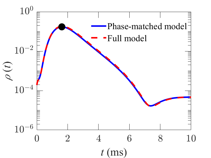
Figure 2: Power ratio $\rho(t)=P_{\rm HOM}(t)/P_{\rm total}(t)$ at the end of the amplifier vs. time t. The pump power equals 250 W.

In Fig. 3, we show $\max[\rho(t)]$ vs. $P_{\rm pump}$ and a dotted line that corresponds to a ratio of 1%. We observe excellent agreement between the phase-matched model and the full model. In this work, we define the threshold power as the lowest pump power at which $\max[\rho(t)]>0.01$, i.e., the ratio of $P_{\rm HOM}(t)/P_{\rm total}(t)$ exceeds 1% at any time. Beyond this threshold, the beam quality rapidly degrades [11, 12, 26, 27]. This definition of the threshold is consistent with studies of amplifier limits due to SBS. In the case considered here, the threshold power equals 207 W.

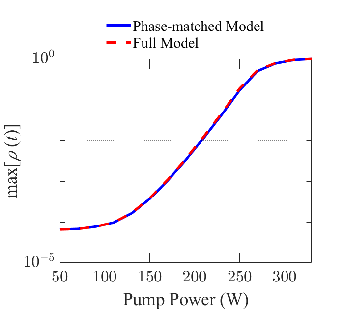
Figure 3: Maximum power ratio $\max[\rho(t)]$ at the amplifier end vs. input pump power $P_{\rm pump}$. The threshold ratio of 1% occurs when $P_{\rm pump}$ = 207 W.

In Fig. 4, we show the temperature as a function of longitudinal position $z$ and the absolute value of its spatial Fourier transform at a distance of 10 $\mu$m from the amplifier center and a time $t=0.5$ ms. We set $P_{\rm pump}=450$ W. In Fig. 4(a), where we show the temperature as a function of position, we see that the agreement between the full model and the phase-matched model appears excellent. In the inset, where we show the spatial oscillations, the two models appear indistinguishable. However, the subtle difference is visible in Fig. 4(b), where we show the absolute value of the spatial Fourier transform, $|\hbox{FT}(T)|=|\int T(z)\exp(ikz)\,dz|$. Agreement is excellent for the central harmonic, as well as the two surrounding harmonics which are located at $k=\pm\Delta\beta=\pm 528$ m^-1. However, the phase-matched model has no contribution from the harmonics at $\pm n\Delta\beta$, where $n\geq 2$. It is precisely these higher harmonics that we are neglecting.

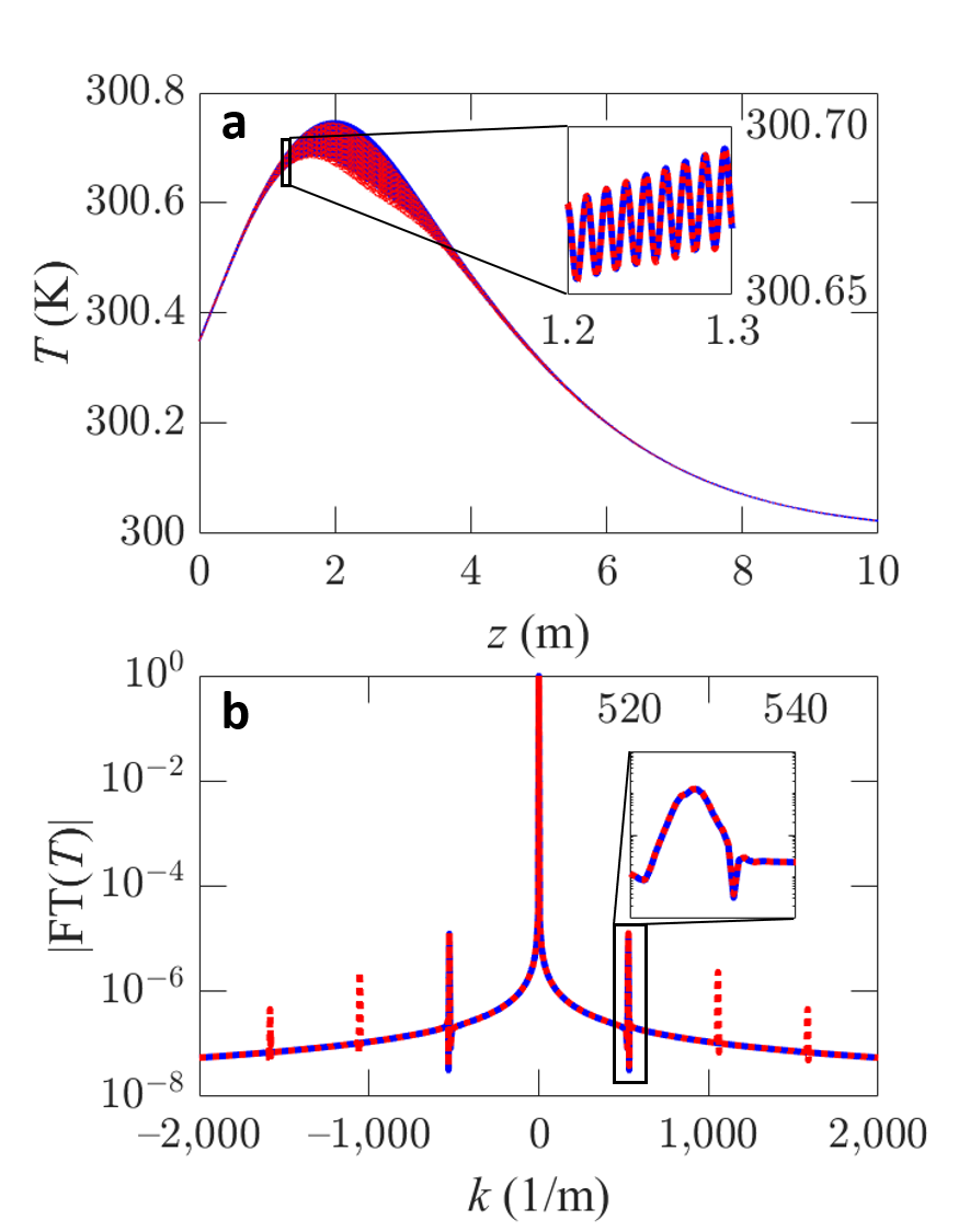
Figure 4: Temperature $T$ at a point that is 10 $\mu$m from the amplifier center when $t=0.5$ ms. (a) $T$ vs. $z$. Agreement is excellent between the full model and the phase-matched model. The inset shows that the details of the temperature oscillations agree. (b) $|$FT($T$)$|$ vs. $k$, where $k$ is the spatial Fourier transform variable. Agreement for the central harmonic and the harmonics at $k=\pm\Delta\beta$ is excellent. The inset shows excellent agreement for the harmonic at $k=\Delta\beta$. However, the harmonics at $k=\pm n\Delta\beta$ for $n\geq 2$ are not present in the phase-matched model.

3.2 Accuracy and Timing

In the phase-matched model, the number of dependent variables is almost twice as large as in the full model. In particular, it is necessary to solve the temperature equation, Eq. (14), for both $T_{0}$ and $T_{+}$ instead of just solving the temperature equation, Eq. (13), for the single temperature $T$. As a result, we have found that the computational load on each $z$-step increases by roughly a factor of two. However, it is possible to take significantly larger steps, leading to a large computational advantage.

In Fig. 5, we show $\max[\rho(t)]$ for both the full model and phase-matched model as a function of $L_{\rm B}/\Delta z$ when $P_{\rm pump}=250$ W, so that the pump power is slightly above threshold. As expected, the full model requires an $L_{\rm B}/\Delta z>60$ to converge, while the phase-matched model appears to have converged in this case when $L_{\rm B}/\Delta z\simeq 2$.

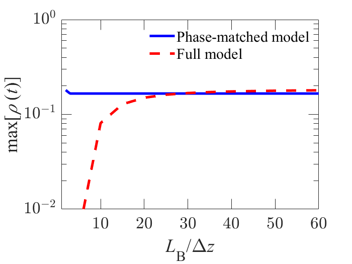
Figure 5: Convergence of the maximum power ratio at the amplifier end as $L_{B}/\Delta z$ increases. We set $P_{\rm pump}=250$ W.

In order to quantify the convergence, we define the relative error, $\epsilon$, as the difference between our computation at a given $\Delta z$ and a four-point Richardson extrapolation [28]. For the full model, we used $L_{\rm B}/\Delta z=80$, 40, 20, and 10 for the extrapolation. For the phase-matched model, we used $L_{\rm B}/\Delta z=40$, 20, 10, and 5.

In Fig. 6(a), we show the relative error as a function of $L_{\rm B}/\Delta z$. We see that achieving a relative error of 1% with the full model requires $L_{\rm B}/\Delta z\simeq 90$, while the same relative error can be obtained with the phase-matched model when $L_{\rm B}/\Delta z\simeq 2$. Figure 6(a) also illustrates that the full model is second-order accurate in $\Delta z$, so that the relative error decreases proportional to $(\Delta z)^{-2}$. This result is consistent with the result of Naderi et al. [19], but may be surprising since our integration in $z$ is done using the Runge-Kutta method. This result indicates that the global error is dominated by the accumulated error in computing the index of refraction. The variation of the relative error in the phase-matched model is more complex since it depends on the rate at which all the dependent variables change as a function of $z$. A complete error analysis is beyond the scope of this paper, but Fig. 6(a) indicates that it decreases rapidly as $\Delta z$ increases until it has become quite small.

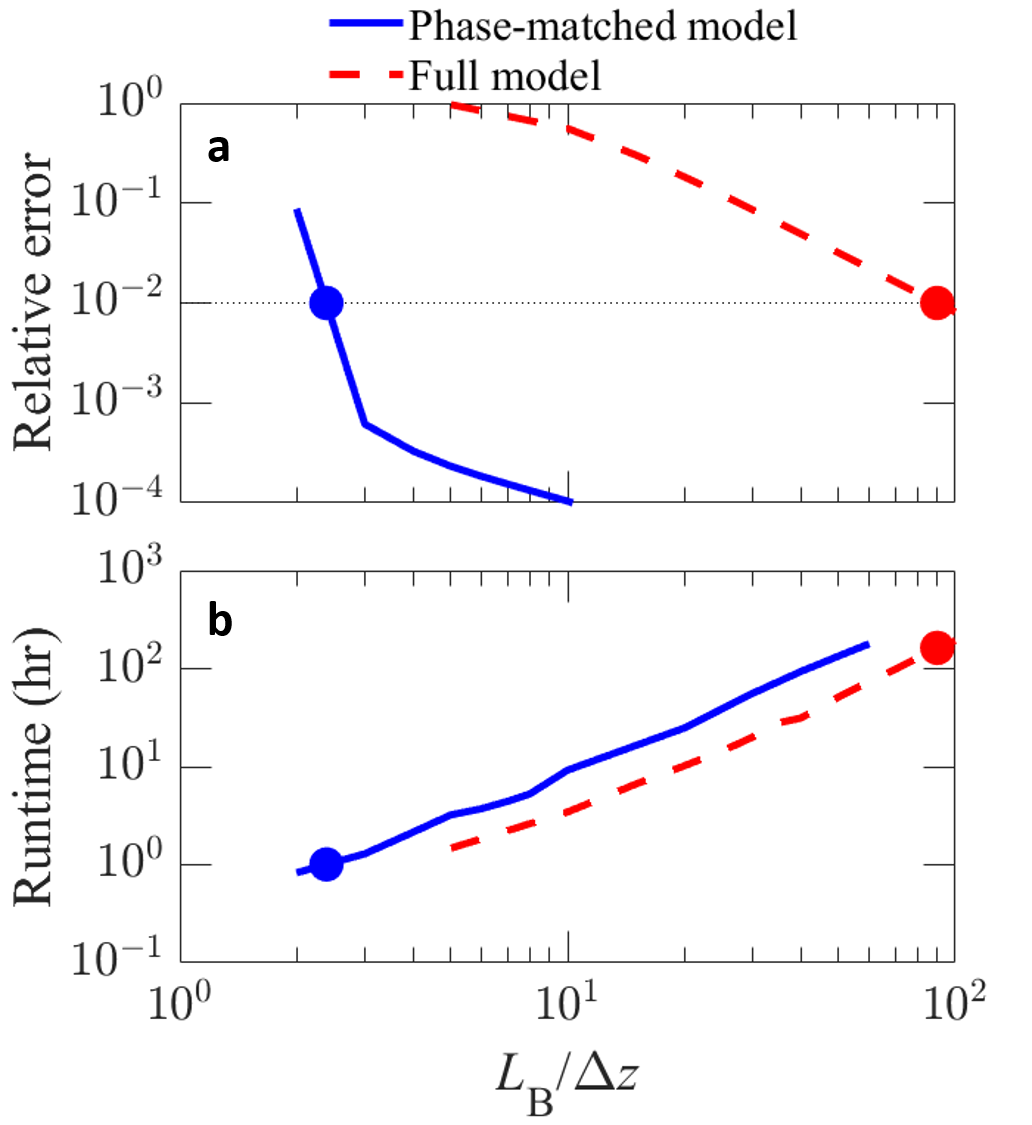
Figure 6: (a) Relative error vs. $L_{B}/\Delta z$ for the cases shown in Fig. 4. (b) Runtime vs. $L_{\rm B}/\Delta z$. The runtime for the phase-matched model is approximately twice as long as the runtime for the full model. Dots indicate the corresponding runtime with a relative error of $1\%$, as shown in Fig. 5.

In Fig. 6(b), we show the runtime of both the full model and the phase-matched model using 16 cores in a shared memory system that consists of dual Intel E5-2695 V4 processors. We observe that the runtime for the phase-matched model is approximately twice as the runtime for the full model, which is consistent with the greater computational load per step in the phase-matched model. When we compare the runtime corresponding to a relative error of 1%, shown with dots, we found a runtime of 163 hours for the full model and 1.17 hours for the phase-matched model, indicating that the phase-matched model runs a factor of 139 faster in this case. While we obtain a speedup of 139 in our study, this number will vary with different simulation parameters. Nevertheless, the advantage of using phase-matched model is clear.

4 Conclusions and Discussion

In this work, we derived the three-wave mixing equations that govern TMI in the limit where a single higher-order mode is present, and the longitudinal rate of change of all quantities is slow compared to the beat length. This limit normally applies in practice. In this limit, TMI can be identified as an STRS process, and we reviewed the theoretical justification for this identification in the appendix, where we also discussed similarities and differences between STRS and SBS in the Appendix. There, we verified the accuracy of the phase-matched model in a Yb³⁺-doped fiber amplifier with a relatively simple step index profile. The amplifier that we considered is like that of Naderi et al. [19], but has a more realistic 10-m length. We demonstrated that this model reproduces the nonlinear saturation of the higher-order mode and the instability threshold that are predicted by the full model. We demonstrated a computational speedup that is more than a factor of 100.

We derived the three-wave mixing equations in the case that a single higher-order mode is present, but we expect this result to be more broadly applicable when several higher-order modes are present. In the linear limit below threshold, each higher-order mode will only interact with the fundamental mode. In that case, the three-wave mixing equations can be extended by adding a new set of equations for the index of refraction, Yb³⁺ population density, heat, temperature, and optical mode amplitude for each of the higher-order modes. The computational complexity scales proportional to $M$, where $M$ is the number of modes. More generally, we anticipate that the three-wave mixing equations can be extended to include a coupling between all the modes as long as none of the beat lengths between any of mode pairs becomes large enough to be comparable to the scale length on which any of the amplitudes change. However, the computational complexity grows proportional to $M^{2}$, and higher-order nonlinear interactions with a slowly varying amplitude could invalidate this approach.

Acknowledgments Work at the Johns Hopkins Applied Physics Laboratory (JHU-APL) and at Baylor University was supported by JHU-APL Internal Research and Development Funds. The authors would like to thank R. A. Lane, J. R. Grosek, and E. J. Bochove at the Air Force Research Laboratory in Kirtland, NM for helpful discussions.

Disclosures The authors declare no conflicts of interest.

Appendix

TMI as an STRS process

The identification of TMI as an STRS process has remained somewhat controversial due to the complexity of TMI. Here, we will briefly argue in favor of this identification in the limit where the phase-matched model holds. We then point out some of the similarities and differences with the instability due to stimulated Brillouin scattering (SBS), which is another important effect limiting the performance of high-energy fiber laser amplifiers [29].

Rayleigh scattering is commonly observed as a spontaneous process. It is well known as the reason the sky is blue [30] and imposes a fundamental loss limit on optical fiber transmission [31]. It also imposes a fundamental limit on fiber interferometers and hence on opto-electronic oscillators [32].

Observation of STRS has proved more elusive, particularly in optical fibers. Zhu et al. [33] reported an observation of STRS in 2010, and Kong et al. [17] reported an observation of STRS in 2016. It is difficult to observe directly, and another observation that was reported in 2012 [34] was later shown to be incorrect [35].

STRS and SBS can be treated together theoretically because both are due to density fluctuations [24]. Rayleigh scattering is driven by isobaric processes, while Brillouin scattering is driven by isentropic processes. Both are three-wave scattering processes in which two optical fields couple to density fluctuations. When Eq. (3) holds, it is evident that TMI can be treated as a three-wave scattering process in which two optical modes couple to density fluctuations and that this process is isobaric. Hence, it is reasonable to identify TMI as an STRS-driven process.

While both STRS and SBS are three-wave processes in which two optical modes couple to density fluctuations, there are important differences—particularly in optical fibers. Rayleigh scattering is often referred to as an inelastic process, but that is almost never strictly true. Energy and momentum conservation implies that there is typically a small frequency offset. In the case of TMI this offset is quite small—on the order of a few kilohertz [13, 14, 15, 16]. This offset plays a critical role in driving the instability, but it lies well within the linewidth of the optical modes, which is typically on the order of 100 MHz. While there is a significant difference between the wavenumbers of the fundamental and higher-order modes, this difference is small compared to the wavenumber of both modes ($\Delta\beta/\beta\sim 10^{-5}$). Both modes propagate in the same direction, but have different mode profiles. By contrast, the two optical modes that become unstable due to SBS are both fundamental modes, but they propagate in opposite directions. As a consequence, the wavenumber offset equals twice the wavenumber of each of the optical modes. The frequency offset, which is given by (the acoustic velocity)$\times$(twice the wavenumber of the optical modes), is of 10–20 GHz and much larger than the linewidth of the optical modes. These differences can be traced to the fundamental physical difference between pressure fluctuations, which propagate, and entropy fluctuations, which do not.

References

- [1] M. N. Zervas and C. A. Codemard, “High power fiber lasers: A review,” \JournalTitleIEEE J. Sel. Topics Quantum Electron. 20, 219–241 (2014).
- [2] D. J. Richardson, J. Nilsson, and W. A. Clarkson,“High power fiber lasers: current status and future perspectives [Invited],” \JournalTitleJ. Opt. Soc. Am. B 27, B63–B92 (2010).
- [3] C. Robin, I. Dajani, and B. Pulford, “Modal instability-suppressing, single-frequency photonics fiber with 811 W output power,” \JournalTitleOpt. Lett. 39, 666–669 (2014).
- [4] L. Dong, F. Kong, G. Gu, T. W. Hawkins, M. Jones, J. Parsons, M. T. Kalichevsky-Dong, K. Saitoh, B. Pulford, and I. Dajani, “Large-mode-area all-solid photonic bandgap fibers for mitigation of optical nonlinearities,” \JournalTitleIEEE J. Sel. Topics Quantum Electron. 22, 4900207 (2016).
- [5] N. A. Naderi, A. Flores, B. M. Anderson, and I. Dajani, “Beam combinable, kilowatt all-fiber amplifier based on phase-modulation gain competition,” \JournalTitleOpt. Lett. 41, 3964–3967 (2016).
- [6] F. Kong, G. Gu, T. W. Hawkins, M. Jones, J. Parsons, M. T. K.-Dong, Stephen P. Palese, E. Cheung, and L. Dong, ”Efficient 240W single-mode 1018nm laser from an Ytterbium-doped 50/400µm all-solid photonic bandgap fiber,” Opt. Express 26, 3138–3144 (2018).
- [7] H. Chen, J. Cao, Z. Huang, Y. Ren, A. Liu, Z. Pan, X. Wang, and J. Chen, “Experimental investigations on multi-kilowatt all-fiber distributed side-pumped oscillators,” Laser Phys. 29, 075103 (2019).
- [8] C. Jauregui, C. Stihler, and J. Limpert, “Transverse mode instability,” Adv. Opt. Photon. 12, 429–484 (2020).
- [9] C. Jauregui, J. Limpert, and A. T unnermann, “High-power fibre lasers,” Nat. Photonics 7, 861–-867 (2013).
- [10] M. Zervas, “Transverse mode instability, thermal lensing, and power scaling in Yb3+-doped high-power fiber amplifiers,” Opt. Exp. 27, 19019–19041 (2019).
- [11] C. Jauregui, T. Eidam, J. Limpert, and A. Tünnermann, “Impact of modal interference on beam quality of high-power amplifiers,” Opt. Exp. 19, 3258–3271 (2011).
- [12] T. Eidam, C. Wirth, C. Jauregui, F. Stutzki, F. Jansen, H.-J. Otto, O. Schmidt, T. Schreiber, J. Limpert, and A. Tünnermann, “Experimental observations of the threshold-like onset of mode instabilities in high power fiber amplifiers,” Opt. Exp. 19, 13218–13224 (2011).
- [13] A. V. Smith and J. J. Smith, “Mode instability in high power amplifiers,” Opt. Exp. 19, 10180–10192 (2011).
- [14] C. Jauregui, T. Eidam, H.-J. Otto, F. Stutzki, F. Jansen, J. Limpert, and A. Tünnermann, “Physical origin of mode instabilities in high-power fiber laser systems,” Opt. Exp. 20, 12912–12925 (2012).
- [15] L. Dong, “Stimulated thermal Rayleigh scattering in optical fibers,” Opt. Exp. 21, 2642–2656 (2013).
- [16] A. V. Smith and J. J. Smith, “Overview of a steady-periodic model of modal instability in fiber amplifiers,” IEEE J. Sel. Topics Quantum Electron. 5, 3000112 (2014).
- [17] F. Kong, J. Xue, R. H. Stolen, and L. Dong, “Direct experimental observation of stimulated thermal Rayleigh scattering with polarization modes in a fiber amplifier,” Optica 3, 975–978 (2016).
- [18] B. Ward, C. Robin, and I. Dajani, “Origin of the thermal mode instabilities in large mode area fiber amplifiers,” Opt. Exp. 20, 11407–11422 (2012).
- [19] S. Naderi, I. Dajani, T. Madden, and C. Robin, “Investigations of modal instabilities in fiber amplifiers through detailed numerical simulations,” Opt. Exp. 21, 16111–16129 (2013).
- [20] B. G. Ward, “Modeling of transient modal instability in fiber amplifiers,” Opt. Exp. 21, 12053–12067 (2013).
- [21] D. Marcuse, Theory of Dielectric Waveguides (Academic, 1991), Chap. 3.2.
- [22] A. W. Snyder and J. D. Love, Optical Waveguide Theory (Chapman and Hall, 1983), Chap. 31.11.
- [23] I. S. Gradshteyn and I. M. Rhyzik, Table of Integrals, Series, and Products (Academic, 1980). See item 3.613.1, p. 366.
- [24] Z. Li, C. Li, Y. Liu, Q. Luo, H. Lin, Z. Huang, S. Xu, Z. Yang, J. Wang and F. Jing, “Impact of stimulated Raman scattering on the transverse mode instability threshold,” IEEE Phot. J. 16, 085109 (2018).
- [25] R. C. Hilborn, “Seagulls, butterflies, and grasshoppers: A brief history of the butterfly effect in nonlinear dynamics,” Am. J. Phys. 72, 425–427 (2004).
- [26] H.-J. Otto, F. Stutzki, F. Jansen, T. Eidam, C. Jauregui, J. Limpert, and A. Tünnermann, “Temporal dynamics of mode instabilities in high-power fiber lasers and amplifiers,” Opt. Exp. 20, 15710–15722 (2012).
- [27] H.-J. Otto, C. Jauregui, F. Stutzki, F. Jansen, and A. Tünnermann, “Controlling instabilities by dynamic mode excitation with an acoustic-optic detector,” Opt. Exp. 21, 19375–19386 (2013).
- [28] W. H. Press et al., Numerical Recipes, 3rd edition (Cambridge, 2007), Ch. 4 and 17.
- [29] J. W. Dawson, M. J. Messerly, R. J. Beach, M. Y. Shverdin, E. A. Stappaerts, A. K. Sridharan, P. H. Pax, J. E. Heebner, C. W. Siders, and C. P. J. Barty, “Analysis of the scalabiity of diffraction-limited fiber lasers and amplifiers to high average power,” Opt. Exp. 16, 13240–13266 (2008).
- [30] See, e.g., M. Born and E. Wolf Principles of Optics (Cambridge, 2005), Chap. 14.5.
- [31] See, e.g., G. Keiser Optical Fiber Communications (McGraw-Hill, 200), Chap. 3.1.3.
- [32] M. Fleyer, J. P. Cahill, M. Horowitz, C. R. Menyuk, and O. Okusaga, “Comprehensive model for studying noise induced by self-homodyne detection of backward Rayleigh schattering in optical fibers,” Opt. Exp. 23, 25635–25652 (2015).
- [33] T. Zhu, X. Bao, L. Chen, H. Liang, and Y. Dong, “Experimental study on stimulated Rayleigh scattering in optical fibers,” Opt. Exp. 18, 22958–22963 (2010).
- [34] O. Okusaga, J. P. Cahill, A. Docherty, W. Zhou, and C. R. Menyuk, “Guided entropy mode Rayleigh scattering in optical fibers,” Opt. Lett. 37, 683–685 (2012).
- [35] O. Okusaga, J. P. Cahill, A. Docherty, C. R. Menyuk, and W. Zhou, “Spontaneous inelastic Rayleigh scattering in optical fibers,” Opt. Lett. 38, 549–551 (2013).