Neuro-Symbolic Constraint Programming for Structured Prediction

Abstract

We propose Nester, a method for injecting neural networks into constrained structured predictors. The job of the neural network(s) is to compute an initial, raw prediction that is compatible with the input data but does not necessarily satisfy the constraints. The structured predictor then builds a structure using a constraint solver that assembles and corrects the raw predictions in accordance with hard and soft constraints. In doing so, Nester takes advantage of the features of its two components: the neural network learns complex representations from low-level data while the constraint programming component reasons about the high-level properties of the prediction task. The entire architecture can be trained in an end-to-end fashion. An empirical evaluation on handwritten equation recognition shows that Nester achieves better performance than both the neural network and the constrained structured predictor on their own, especially when training examples are scarce, while scaling to more complex problems than other neuro-programming approaches. Nester proves especially useful to reduce errors at the semantic level of the problem, which is particularly challenging for neural network architectures.

1 Introduction

Neural networks have revolutionized several sub-fields of AI, including computer vision and natural language processing. Their success, however, is mainly limited to “perception” tasks, where raw unstructured data is abundant and prior knowledge is scarce or not useful (?). Standard deep networks indeed rely completely on inductive reasoning to acquire complex patterns from massive datasets. This approach cannot be straightforwardly applied to machine learning problems characterized by limited amounts of highly structured data. Solving these tasks requires to generalize from few examples by leveraging background knowledge, which in turn involves applying inductive and deductive reasoning. This observation has prompted researchers to develop neuro-symbolic models that integrate deep learning with higher level reasoning (?; ?; ?; ?; ?).

We tackle neuro-symbolic integration in the context of structured output prediction under constraints. In regular structured output prediction, the goal is to predict a structured object encoded by multiple interdependent and mutually constrained output variables (?). Examples include parse trees, floor plans, game levels, molecules, and any other functional objects that must obey validity constraints (?; ?).

Our setting is more complex than regular structured prediction in that it involves predicting structures i) subject to complex logical and numerical constraints, ii) from sub-symbolic inputs like images or sensor data. This problem is beyond the reach of existing methods. Classical frameworks for structured prediction (?; ?) lack any functionality for representation learning, which is a key component for handling sub-symbolic data. Most deep structured prediction approaches, on the other hand, do not support explicit constraints on the output, neither hard nor soft (?; ?). Existing neuro-symbolic approaches combining logical constraints and deep learning either rely on fuzzy logic (?; ?; ?) or enforce satisfaction of constraints only in expectation (?), in both cases failing to deal with hard constraints. Furthermore, these approaches are usually restricted to logical constraints. The most expressive approach in this class is DeepProbLog (?), which enriches the probabilistic programming language ProbLog with neural predicates and is designed to process sub-symbolic data together with logic and (discrete) numeric constraints. However, probabilistic inference in DeepProbLog can become prohibitively expensive when dealing with structured prediction problems with a high degree of non-determinism, as highlighted by our experiments.

We propose Nester (NEuro-Symbolic consTrainEd structuRed predictor), a hybrid approach that integrates neural networks and constraint programming to effectively address constrained structured prediction with sub-symbolic inputs and complex constraints. Nester combines a neural model with a constrained structured predictor into a two-stage approach. On the one hand, the neural network processes low-level inputs (e.g., images) and produces a raw candidate structure based on the data alone. This intermediate output acts as a initial guess and may violate one or more of the hard constraints. On the other, the structured predictor refines the network’s outputs and leverages a constraint satisfaction solver to impose hard and soft constraints on the final output. Inspired by work on declarative structured output prediction (?; ?), Nester leverages the mid-level constraint programming language MiniZinc (?) to define the constraint program, thus inheriting the latter’s ability to deal with hard and soft constraints over categorical and numerical variables alike. The entire architecture can be trained end-to-end by backpropagation.

We evaluated Nester on handwritten equation recognition (?), a sequence prediction task in which the prediction must obey both syntactic and semantic constraints, cf. Figure 1. Our results show that the neural network and the constrained structured predictor work in synergy, achieving better results than either model taken in isolation. Importantly, while the neural network alone can rather easily learn the correct syntax for the output, it struggles to achieve low error at the semantic level of the problem. Our combined architecture, on the other hand, outputs predictions that are both syntactically sound and semantically valid.

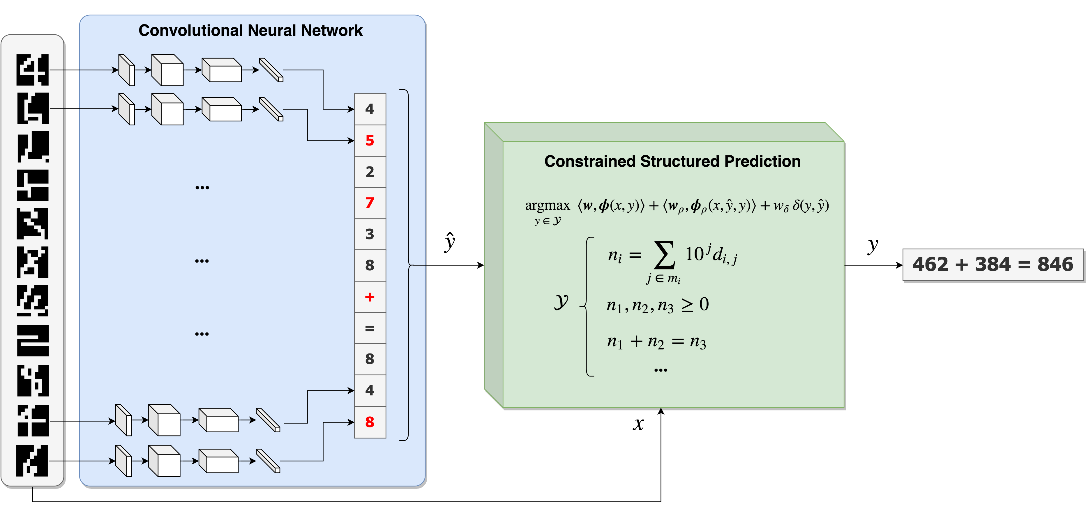
Figure 1: Architecture of the proposed model in the handwritten equation recognition setting. The figure shows the procedure for predicting an instance, i.e. a sequence of images forming an equation. Each image is first classified by a CNN (the same network for each image), and the predicted labels are grouped into a sequence $\hat{y}$. The structured predictor then takes the sequence $x$ and the intermediate prediction $\hat{y}$ and predicts a label $y$ by solving a structured prediction problem with the imposed constraints. Note how the network output $\hat{y}$ violates both syntactic and semantic constraints, while the final output $y$ is guaranteed to satisfy both. Best viewed in colors.

2 Structured Prediction under Constraints

In structured prediction the goal is to predict an output structure from an input, also typically structured. Standard examples include part-of-speech tagging or protein secondary structure prediction, where input and output are sequences of symbols, or parse tree prediction, where a tree structure should be predicted starting from an input sequence. Directly learning a mapping function $f:\mathcal{X}\to\mathcal{Y}$ is tricky given the structured nature of $\mathcal{Y}$. Approaches to deal with the problem fall in two main categories. Energy-based prediction models (?) rely on a function $F:\mathcal{X}\times\mathcal{Y}\to\mathbb{R}$ that computes the compatibility between input and output. Learning aims at maximizing the score (or minimizing the energy) of the correct output for a given input, so that inference can be computed by maximizing the function over the output space:

$$y=\operatorname*{argmax}_{y^{\prime}\in\mathcal{Y}}F(x,y^{\prime})$$ (1)

Search-based models (?; ?) frame structured prediction as a search in the space of candidate outputs, where a scoring function evaluates the quality of a certain move (e.g., labeling the next output in the sequence) given the current state (the input and the labels predicted for the previous elements). Search-based models are typically more efficient than energy-based ones, as they do not need to run inference over the entire structure. On the other hand, by jointly inferring the entire structure, energy-based models can naturally incorporate hard constraints over the output structure. Indeed, while soft constraints between output variables (e.g., the propensity for a verb to follow a noun) can be implicitly learned by both framework in terms of weights associated to states or input-output pairs, long-range hard constraints (e.g., non-overlap in furniture layouts (?), playability in game level generation (?)) are challenging for search-based models as they would require complex backtracking operations to retain satisfaction of the constraint. The severity of the problem depends on the scope of the constraint, with global (even soft) constraints being much harder to manage than local ones. We thus focus on energy-based models in this paper.

Structured SVM (?; ?) is a popular energy-based model, that has the advantage of carrying generalization guarantees of SVM to the structured prediction setting. In structured SVM, $F(x,y)$ is modelled as a linear function of the type $\langle\bm{\mathrm{w}},\bm{\mathrm{\phi}}(x,y)\rangle$, where $\bm{\mathrm{\phi}}:\mathcal{X}\times\mathcal{Y}\to\mathbb{R}^{d}$ is a feature map that transforms input-output pairs into a $d$-dimensional joint feature space, and $\bm{\mathrm{w}}\in\mathbb{R}^{d}$ is a parameter vector to be learned from data. Given a training set of $n$ input-output pairs $\{(x_{i},y_{i})\}_{i=1}^{n}$, where $y_{i}$ is a high-quality output for $x_{i}$, structured SVM learn $\bm{\mathrm{w}}$ by solving the following quadratic problem:

$$\min_{\bm{\mathrm{w}},\bm{\mathrm{\xi}}}\quad \frac{\lambda}{2}\lVert\bm{\mathrm{w}}\rVert^{2}+\frac{1}{n}\sum_{i=1}^{n}\xi_{i}$$ (2)

s.t. $$\forall\ i\in[n],y\in\mathcal{Y}\setminus\{y_{i}\}$$

$$\langle\bm{\mathrm{w}},\bm{\mathrm{\phi}}(x_{i},y_{i})\rangle-\langle\bm{\mathrm{w}},\bm{\mathrm{\phi}}(x_{i},y)\rangle\geq\Delta(y_{i},y)-\xi_{i}$$

The inequality constraints encourage the scoring function to rank the correct label above all the others. In particular, for each training pair $(x_{i},y_{i})$, they ensure that the score of the correct label $\langle\bm{\mathrm{w}},\bm{\mathrm{\phi}}(x_{i},y_{i})\rangle$ is larger than the score of any other label by at least $\Delta(y_{i},y)$, the latter being a task-dependent loss that measures how much $y$ differs from $y_{i}$. These constraints are soft, and the slack variables $\bm{\mathrm{\xi}}\in\mathbb{R}^{n}$ are penalties for not satisfying them. The objective to be minimized combines the slacks with and an $\ell_{2}$ regularization term $\frac{\lambda}{2}\lVert\bm{\mathrm{w}}\rVert^{2}$ that encourages simplicity and generalization. Many algorithms have been developed for solving Eq. 1 including cutting plane (?) and block-coordinate Frank-Wolfe (?). In this work we rely on stochastic sub-gradient descent (?), as it can be extended to deep models, as discussed in the next section. Stochastic sub-gradient descent for structured SVM works by minizing the structured hinge loss:

$$L(\bm{\mathrm{w}};x_{i},y_{i},y^{*}_{i})=\frac{\lambda}{2}\lVert\bm{\mathrm{w}}\rVert^{2}+\langle\bm{\mathrm{w}},\bm{\mathrm{\phi}}(x_{i},y^{*}_{i})-\bm{\mathrm{\phi}}(x_{i},y_{i})\rangle$$

where

$$y^{*}_{i}=\operatorname*{argmax}_{y\in\mathcal{Y}}\;\Delta(y_{i},y)-\langle\bm{\mathrm{w}},\bm{\mathrm{\phi}}(x_{i},y_{i})-\bm{\mathrm{\phi}}(x_{i},y)\rangle$$

Given $y^{*}_{i}$, it is possible to compute the sub-gradient $\nabla_{\bm{\mathrm{w}}}L$ and then follow its direction via a standard gradient descent step or variants thereof.

Depending on the model structure and output space $\mathcal{Y}$, the hardness of computing a prediction (Equation 1) varies greatly. If the output objects $y\in\mathcal{Y}$ are composed of real variables only and the space $\mathcal{Y}$ is convex, then a prediction can be computed using gradient-based optimization methods. Discrete variables render the task much more challenging. Most research on structured prediction of discrete objects has focused on problems for which an efficient prediction algorithm is known, such as the Viterbi algorithm for sequences and the inside-outside algorithm for trees, or has resorted to approximate inference (?) that does not guarantee satisfaction of hard constraints. Following recent improvements of constraint solving technologies, it has become increasingly more feasible to delegate the job of solving the inference problem in Equation 1 to a generic constraint solver (?). Nowadays, mixed integer linear programming frameworks can solve optimization problems with several hundred variables in a matter of milliseconds. Constraint programming languages such as MiniZinc (?) have also been leveraged in structured prediction problems involving complex output structures (?), such as layout synthesis (?) and product bundling recommendation (?). Constraint programming is particularly well suited for encoding structured prediction tasks, as it allows to easily embed background knowledge directly into the predictor in the form of arbitrary logic and algebraic constraints. For instance, in the equation recognition task described in this paper, we are able to easily encode the fact that equations must be valid by specifying constraints that transform the sequence of labels into integers and another constraint defining the relationship between these integers (more details in Section 5).

3 Neural Constrained Structured Prediction

A substantial limitation of approaches based on structured SVM is that they are shallow, leaving to the user the burden of designing appropriate joint feature mappings $\phi$. On the other hand, the ability to learn effective representations from low-level data is a key reason for the success of deep learning technology. Indeed, deep structured prediction has become predominant in domains like NLP (?) which are characterized by an abundance of labelled data. The standard solution to apply neural approaches to structured prediction problems is that of search-based learning, where auto-regressive models like LSTM or attention-based models are employed to predict the next output given the subset of already predicted ones. This solution however suffers from a number of problems (?), like the so-called exposure bias (during training, the ground-truth is assumed for the subset of already predicted variables) and the discrepancy between the training loss (cross entropy on the label of the next output) and the task loss (quality of the overall output prediction). While several ad-hoc solutions have been developed to try addressing these problems, by adapting techniques developed for shallow search-based structured prediction (?), these approaches share with their shallow counterparts the lack of support for hard constraints. Deep energy-based approaches have also been explored (?; ?). However they rely on gradient-based inference in a relaxed output space, and thus again they cannot satisfy constraints. Indeed, satisfaction of constraints has been indicated as one of the major challenges for deep structured prediction (?).

To solve this issue, we propose Nester, a neural constrained structured prediction model. Nester features a general-purpose constrained structured predictor (?) (see Section 2) that acts as a “refinement” layer on top of the predictions made by a standard neural network. The constrained structured predictor is fed both the input $x\in\mathcal{X}$ and the predictions of the neural network $\hat{y}\in\mathcal{Y}$, and outputs a final prediction $y\in\mathcal{Y}$. Figure 1 shows, as an example, the architecture that has been used in our experiments on handwritten equation recognition (see Section 5), but different architectures may be used depending on the domain. Note that the neural network does not have to be aware of the structure of the output, and may even simply predict the output variables independently. The constrained structured predictor is in charge of grouping the predictions into the desired structure while “correcting” the mistakes of the network and enforcing the constraints of the problem. To do so, both hard and soft constraints are encoded in the constraint program. The former represent hard requirements that the output needs to satisfy in order to be considered valid (e.g., algebraic constraints for handwritten equation recognition). The latter represent features defined over a combination of inputs, network outputs and refined outputs, which potentially correlate with the correctness of the refinement, and whose weights are learned during training.

More specifically, prediction consists in solving the following constrained optimization program:

$$\operatorname*{argmax}_{y\in\mathcal{Y}} \langle\bm{\mathrm{w}},\bm{\mathrm{\phi}}(x,y)\rangle+\langle\bm{\mathrm{w}}_{\rho},\bm{\mathrm{\phi}}_{\rho}(x,\hat{y},y)\rangle+w_{\delta}\,\delta(y,\hat{y})$$

s.t. $$\hat{y}=g(x;W)$$

where $\mathcal{Y}$ encodes the hard constraints, $g(x;W)$ is an arbitrary neural network (ignoring the constraints), $\bm{\mathrm{\phi}}(x,y)$, $\bm{\mathrm{\phi}}_{\rho}(x,\hat{y},y)$ and $\delta(y,\hat{y})$ are features, and $(\bm{\mathrm{w}},\bm{\mathrm{w}}_{\rho},w_{\delta})$ and $W$ are learnable weights of the constrained structured predictor and the neural network respectively. We refer to $\bm{\mathrm{\phi}}(x,y)$ as prediction features, whereas $\bm{\mathrm{\phi}}_{\rho}(x,\hat{y},y)$ are named refinement features. The former are features that help predicting the right output from the input, analogously to the ones used in standard structured prediction models (?). The latter are features that should help spotting the common mistakes made by the network, by relating input, output and network predictions. Finally $\delta(y,\hat{y})$ represents a distance measure between the prediction of the structured predictor and the one of the neural network and, depending on $w_{\delta}$, acts as a regularizer, preventing the structured predictor from learning to make predictions too dissimilar from the neural network.

Learning the combined model can be done in three steps:

1. If possible, pre-train the neural network; as mentioned, the neural network does not have to be aware of the output structure, so if the structured labels can be deconstructed into the basic output components of the neural network then the network can be pre-trained using those.

2. Train the constrained structured prediction model. At this stage, the structured predictor is trained independently from the neural network and it gets the predictions of the neural network as if they were any other inputs.

3. Fine tune the constrained structured predictor and the neural network end-to-end, using stochastic sub-gradient descent and back-propagating the gradient of the structured hinge loss through the structured model and through the network.

The last point can be achieved by simply chaining the gradients of the structured hinge loss with respect to $\hat{y}$ and the gradient of the neural network output with respect to its weights. For the last layer of the network with weights $W_{K}$:

$$\nabla L=\left[\frac{\partial L}{\partial\hat{y}}\frac{\partial\hat{y}}{\partial W_{K}}\right]$$

Gradients for the other layers can be obtained by standard backpropagation through the network, chaining gradients over the layers starting from the last one.

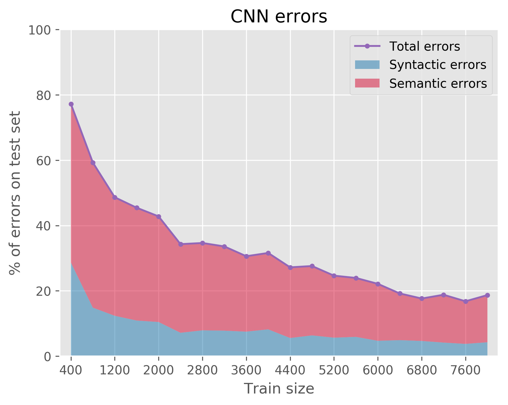
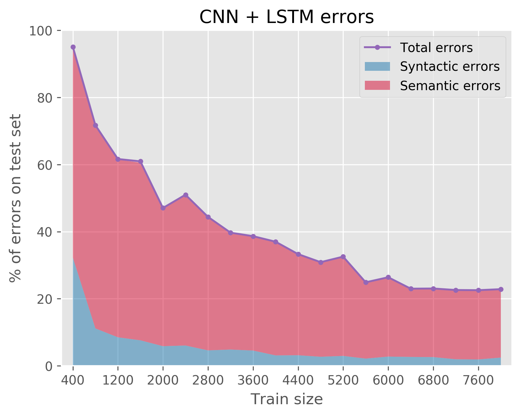
Figure 2: Percentage of erroneously predicted equations by the CNN (left) and by the CNN + LSTM (right) on the test set with increasing training set size. The plots show the percentage of total errors over the test set size and its decomposition into syntactic and semantic errors. Best viewed in colors.

4 Neural constrained sequence prediction

In the rest of the paper, we will focus on a common kind of structured prediction problem, namely sequence prediction. In (discrete) sequence prediction, the objects to predict are sequences of varying length $m$, i.e. $y=(y_{1},\dots,y_{m})$, and each element $y_{j}$ of the sequence takes values from an alphabet of $q$ possible symbols $\{s_{k}\}_{k=1}^{q}$. For each element of the sequence, a vector of $l$ input features is typically available. We indicate with $x_{e,i}$ the $i$-th feature of the $e$-th element of the input sequence.

As prediction features we employ standard features for correlating input and output variables commonly used in e.g. conditional random fields (?) for sequence prediction. These come in the form of two vectors, and are referred as emission and transition features. The former are encoded as:

$$\phi_{i,k}(x,y)=\sum_{e=1}^{m}x_{e,i}\cdot\llbracket y_{e}=s_{k}\rrbracket$$ (3)

where $i$ ranges over input features and $k$ over output symbols, and the expression $\llbracket\cdot\rrbracket$ equals to $1$ if the argument is true, $0$ otherwise. The resulting vector can then be used to correlate the appearance of a specific pixel inside input images with each of the emitted symbols. The transition features are define as follows:

$$\phi_{k_{1},k_{2}}(x,y)=\sum_{e=1}^{m-1}\llbracket y_{e}=s_{k_{1}}\ \land\ y_{e+1}=s_{k_{2}}\rrbracket$$ (4)

where $k_{1},k_{2}$ ranges over all the possible combinations of couples of symbols, counting the number of times in which two symbols appear one after the other. This formulation enables the predictor to correlate the appearance of consecutive symbols inside the output sequence.

The refinement features, on the other hand, need to correlate mistakes of the network with the input and output variables. For this sequence prediction task, we define the refinement features vector $\bm{\mathrm{\phi}}_{\rho}$ as:

$$\phi_{i,k}(x,\hat{y},y)=\sum_{e=1}^{m}x_{e,i}\cdot\llbracket y_{e}=s_{k}\ \land\ \hat{y}_{e}\neq s_{k}\rrbracket$$ (5)

where $i$ ranges over input features and $k$ over output symbols. These features basically correlate the values of each input feature with the overriding of neural network predictions by the refinement layer. By learning appropriate weights for them, the structured predictor can learn to fix the most common mistakes made by the neural network. Finally, we define $\delta(y,\hat{y})$ as the Hamming distance between $y$ and $\hat{y}$:

$$\delta(y,\hat{y})=\sum_{e=1}^{m}\llbracket y_{e}\neq\hat{y}_{e}\rrbracket$$

Table 1 contains an overview of all the components of the constrained problem we used in our experiments.

5 Experiments

We tested our technique on the handwritten equation recognition task described in (?). All our experiments are implemented using Tensorflow and Pyconstruct (?). MiniZinc (?) was used as constraint programming engine and Gurobi as the underlying constraint solver. The code of Nester will be made available upon acceptance.

5.1 Setting

Each input object is a sequence of images of variable length, and the corresponding output is a sequence of symbols of the same length. The possible symbols include the digits from $0$ to $9$, $+$ and $=$. The equations are all of the form $a+b=c$, where $a,b,c$ are arbitrary positive integers (of a predefined maximum number of digits), and the equations are all valid, meaning that it is always true that $a$ plus $b$ equals $c$. This is the background knowledge of the problem. Images are matrices of $9\times 9$ black and white pixels. The dataset was constructed by assembling 10,000 valid equations from the ICFHR’14 CROHME competition data. All our experiments were run on the same train-test split, consisting of 8,000 equations for training and 2,000 for testing. To highlight the behavior of the models with different amounts of training examples, we divided the training set into 20 chunks of increasing size and report results over the test set for each training set chunk.

5.2 Neural model

As highlighted in Figure 1, we use a CNN to predict the symbol of each image in the sequence independently. The CNN is composed of two convolutional layers with $3\times 3$ filters and ReLU activation, each followed by a $2\times 2$ max-pool layers, then a $128$ dense layer with dropout regularization ($0.5$ probability), and finally a softmax layer with $12$ outputs, one for each symbol. The CNN is trained using Adam (?) with a cross entropy loss.

The left plot in Figure 2 reports the relative misclassification error of the CNN over the test set, i.e. the percentage of sequences for which the network made at least one mistake. The violet line indicates the total percentage of errors across the various training set chunks. As the network does not enforce any constraint on the output, it is subject to errors resulting from predicting inconsistent output objects. We subdivide the constraint satisfaction errors into syntactic errors, for which the prediction is not properly formatted according to the template $a+b=c$, and semantic errors, i.e. well-formatted predictions for which the resulting equation is not valid, that is $a$ plus $b$ does not equal $c$. Occasionally the network makes mistakes that are not due to unsatisfied constraints, but these are a very slim minority. The shaded areas in Figure 2 show how the different types of errors contribute to the total. While the total number of errors decreases with increasing training set size, the proportion between syntactic and semantic errors settles around $33\%$ to $67\%$, indicating that semantic errors are generally harder to correct. To make sure that these errors are not simply due to the fact that the CNN predicts each output symbol independently, we also experimented with a recurrent architecture. The recurrent network is assembled by stacking over each convolutional layer of our CNN an LSTM layer. Differently from the CNN, the network is trained with whole input-output sequence pairs.

The right plot in Figure 2 shows the errors of this architecture and their decomposition into syntactic and semantic types. Overall, the network made more errors, possibly due to the increased number of trainable parameters and thus the necessity for more examples to be properly trained. Relatively speaking, though, the CNN + LSTM network learned very quickly how to fix syntactic errors, even faster than the CNN. Yet, semantic errors were much more difficult to correct, and they ended up being the large majority of the errors of the network. These results show that even highly-expressive neural network architectures can have problems in going beyond the shallow syntactic level and reach a deeper semantic level of understanding, especially when limited data is available.

5.3 Constrained structured model

As constrained structured layer (“CST” from now on) we used an enhanced version of the constrained model from (?). Not being conceived to refine predictions from other modules, the original model only contains prediction features $\bm{\mathrm{\phi}}(x,y)$. Our model extends the original one by taking the prediction of the neural network $\hat{y}$ as input, combining the prediction features with the refinement features described in Equation 5, and including the Hamming distance between $y$ and $\hat{y}$ (see Figure 1). A summary of the features and constraints used in the structured predictor is given in Table 1.

Table 1: Summary of the components of the constrained structured predictor in the handwritten equation recognition setting. The expression $\llbracket\cdot\rrbracket$ equals to $1$ if the argument is true, $0$ otherwise.

Input  $x,\hat{y}$

$\circ\$ Array of $m$  $9\times 9$ images, of $\{0,1\}$ pixels

$x\in\{0,1\}^{m\times 9\times 9}$

where

$x_{e,i,j}\in\{0,1\}$  $(i,j)$-th pixel of the $e$-th image

$\circ\$ Array of $m$ predictions of the neural network (NN)

$\hat{y}\in\{0,\dots,q\}^{m}$

where

$q=11$ $\implies$ digits: 0-9,  plus ($+$): $10$,  equals ($=$): $11$

$\hat{y}_{e}\in\{0,...,q\}$  NN prediction for the $e$-th image

Output  $y$

$\circ\$ Array of $m$ output symbols

$\qquad y\in\{0,...,q\}^{m}$

where

$q=11$ $\implies$ (same as above)

$y_{e}\in\{0,...,q\}$  output symbol for the $e$-th image

Prediction features  $\bm{\mathrm{\phi}}(x,y)$

$\circ\$ Emission features: appearance of a pixel in images of a class,

$\qquad\phi_{i,j,k}(x,y)=\sum_{e=1}^{m}x_{e,i,j}\cdot\llbracket y_{e}=k\rrbracket$

where

$k\in\{0,\dots,11\}$ ranges over symbols

$(i,j)\in\{0,\dots,9\}^{2}$ range over pixels

$\circ\$ Transition features: classes in contiguous images,

$\qquad\phi_{k_{1},k_{2}}(x,y)=\sum_{e=1}^{m-1}\llbracket y_{e}=k_{1}\ \land\ y_{e+1}=k_{2}\rrbracket$

where

$(k_{1},k_{2})\in\{0,\dots,11\}^{2}$ range over pairs of symbols

Refinement features  $\bm{\mathrm{\phi}}_{\rho}(x,\hat{y},y)$

$\circ\$ Disagreement between the network prediction and the output,

$\qquad\phi_{i,j,k}(x,\hat{y},y)=\sum_{e=1}^{m}x_{e,i,j}\cdot\llbracket y_{e}=k\ \land\ \hat{y}_{e}\neq k\rrbracket$

where

$k\in\{0,\dots,11\}$ ranges over symbols

$(i,j)\in\{0,\dots,9\}^{2}$ range over pixels

Distance measure  $\delta(\hat{y},y)$

$\circ\$ Hamming distance between output and network prediction

$\qquad\delta(y,\hat{y})=\sum_{e=1}^{m}\llbracket y_{e}\neq\hat{y}_{e}\rrbracket$

The definition of the constrained structured model is presented in the MiniZinc code listed in Figure 3. The sequence of images composing the equation is given as input. The output consists of a sequence of symbols equal to the length of the input sequence, each symbol being an integer between zero and eleven (0-9 for the digits, 10 and 11 for the $+$ and $=$ operators respectively). The input also contains the sequence of symbols predicted by the CNN.

⬇

1%% ~~~~~~~~~~~~~~~~~~~~~~~~~~ INPUT/OUTPUT ~~~~~~~~~~~~~~~~~~~~~~~~ %%

2%% Max digits per number, dimension of the images (9 x 9)

3int: DIGITS = 3;

4set of int: HEIGHT = 1 .. 9; set of int: WIDTH = 1 .. 9;

5

6%% Assume "+" is encoded by 10 and "=" is encoded by 11

7set of int: SYMBOLS = 0 .. 11; int: PLUS = 10; int: EQ = 11;

8

9%% INPUT: sequence length, tensor of images, CNN prediction

10int: len; set of int: SEQ = 1 .. len;

11array[SEQ, HEIGHT, WIDTH] of {0, 1}: img;

12array[SEQ] of SYMBOLS: cnn_seq;

13

14%% OUTPUT: sequence of symbols

15array[SEQ] of var SYMBOLS: seq;

16

17%% ~~~~~~~~~~~~~~~~~~~~~~~~ DOMAIN KNOWLEDGE~~~~~~~~~~~~~~~~~~~~~~~ %%

18%% Indices of the two operators

19array[1 .. 2] of var 2 .. (length - 1): opr;

20

21%% Syntactic constraints: exactly one "+" and one "=", "+" before "=",

22%% positions corresponding to indices "opr" in the sequence

23constraint count(seq, PLUS, 1) /\ count(seq, EQ, 1);

24constraint increasing(opr) /\ seq[opr[1]] == PLUS /\ seq[opr[2]] == EQ;

25

26%% Extremes and number of digits of the three numbers

27array[1 .. 4] of var 0 .. len + 1: ext = [0, opr[1], opr[2], len + 1];

28array[1 .. 3] of var 1 .. DIGITS: n_digits = [

29 ext[i + 1] - ext[i] - 1 | i in 1 .. 3 ];

30

31%% Matrix of digits, zero-padded on the left if less than three digits

32array[1 .. 3, 1 .. DIGITS] of var SYMBOLS: digits =

33 array2d(1 .. 3, DIGITS, [

34 if j <= (DIGITS - n_digits[i]) then 0 else

35 seq[ext[i] + j + n_digits[i] - DIGITS]

36 endif

37 | i in 1 .. 3, j in 1 .. DIGITS ]);

38

39%% The three numbers, sum digits for corresponding power of 10

40array[1 .. 3] of var int: num = [

41 sum(j in 1 .. DIGITS)(pow(10, DIGITS - j) * digits[i, j])

42 | i in 1 .. 3 ];

43

44%% Semantic constraint: the equation must be valid

45constraint num[1] + num[2] == num[3];

46

47%% ~~~~~~~~~~~~~~~~~~~~~~~~~~~~ FEATURES ~~~~~~~~~~~~~~~~~~~~~~~~~~~~ %%

48%% EMISSION + TRANSITION + REFINEMENT + DISTANCE

49int: N_FEATURES = 9*9*12 + 12*12 + 9*9*12 + 1;

50

51array[1 .. N_FEATURES] of var int: features =

52 %% EMISSION FEATURES

53 [ sum(e in SEQ)(img[e, i, j] * (seq[e] == s))

54 | i in HEIGHT, j in WIDTH, s in SYMBOLS ]

55 %% TRANSITION FEATURES

56++ [ sum(e in 1..len - 1)(seq[e] == s1 /\ seq[e + 1] == s2)

57 | s1, s2 in SYMBOLS ]

58 %% REFINEMENT FEATURES

59++ [ sum(i in SEQ)(img[i, j, k] * (seq[i] == s) * (cnn_seq[i] != s))

60 | j in HEIGHT, k in WIDTH, s in SYMBOLS ]

61 %% HAMMING DISTANCE

62++ [ -sum(i in SEQ)(cnn_seq[i] != seq[i]) ];

Figure 3: A sketch of the MiniZinc program for the constrained structured model for the equation recognition problem. The MiniZinc program encodes the input images tensor, and neural network predictions (lines 10-12) and the output sequence of symbols (line 15), the domain knowledge in the form of hard constraints ensuring the equation is properly syntactically formatted (lines 18-29) and enforcing the semantic validity of the equation (lines 31-45), and finally the features of the structured model as defined in Equation 3, prediction features (lines 52-57), refinement features (lines 58-60) and distance metric (lines 61-62), whose weights are learn from data. For brevity, the figure omits some parts regarding the definition of the weights and the objective function. Best viewed in color.

Syntactic constraints over the output are encoded in lines $23$ and $24$. They enforce the presence of a single $=$ and a single $+$ in the output sequence, plus the constraint that the $+$ symbol should come before the $=$ one. The next code section (from line $26$ to $42$) is devoted to converting the sequence of output symbols into an actual algebraic formula. This procedure starts in line $27$ with the definition of the extremes of the three numbers, that are given by the two operators. The extremes are used to count the number of digits that compose each of the three numbers (lines $28$-$29$). These two pieces of information, coupled with the sequence predictions, are then used in lines $32$-$37$ to populate a $3\times 3$ matrix, where each row represents one of the three numbers, and the columns represent the digits, sorted from the most significant to the least significant. Each number can be composed at most by $3$ digits, if the digits are less than $3$, the number is left padded with the appropriate number of zeros. The matrix is then transformed into $3$ integer values $a$, $b$ and $c$ (lines $40$-$42$), summing up all digits of each row, multiplied by the appropriate power of $10$, according to their relative position. In formula, each row $i$ is converted into an integer $n_{i}=\sum_{0\leq j<m_{i}}10^{j}\cdot d_{i,j}$, where $m_{i}$ is the number of digits in number $i$ and $d_{i,j}$ is the $j$-th digit of the $i$-th number, from the least to the most significant digit. This conversion allows us to impose in line $45$ the semantic constraint enforcing the output sequence to encode a valid formula, i.e. $a+b=c$.

The last section of the code is devoted to declaring the features, with the formulation introduced in Section 3 (from line $47$ to $62$). This code is a template that Pyconstruct (?) uses to solve different inference problems during training and prediction. At runtime, the library takes care of determining which objective function to optimize depending on the inference problem at hand.

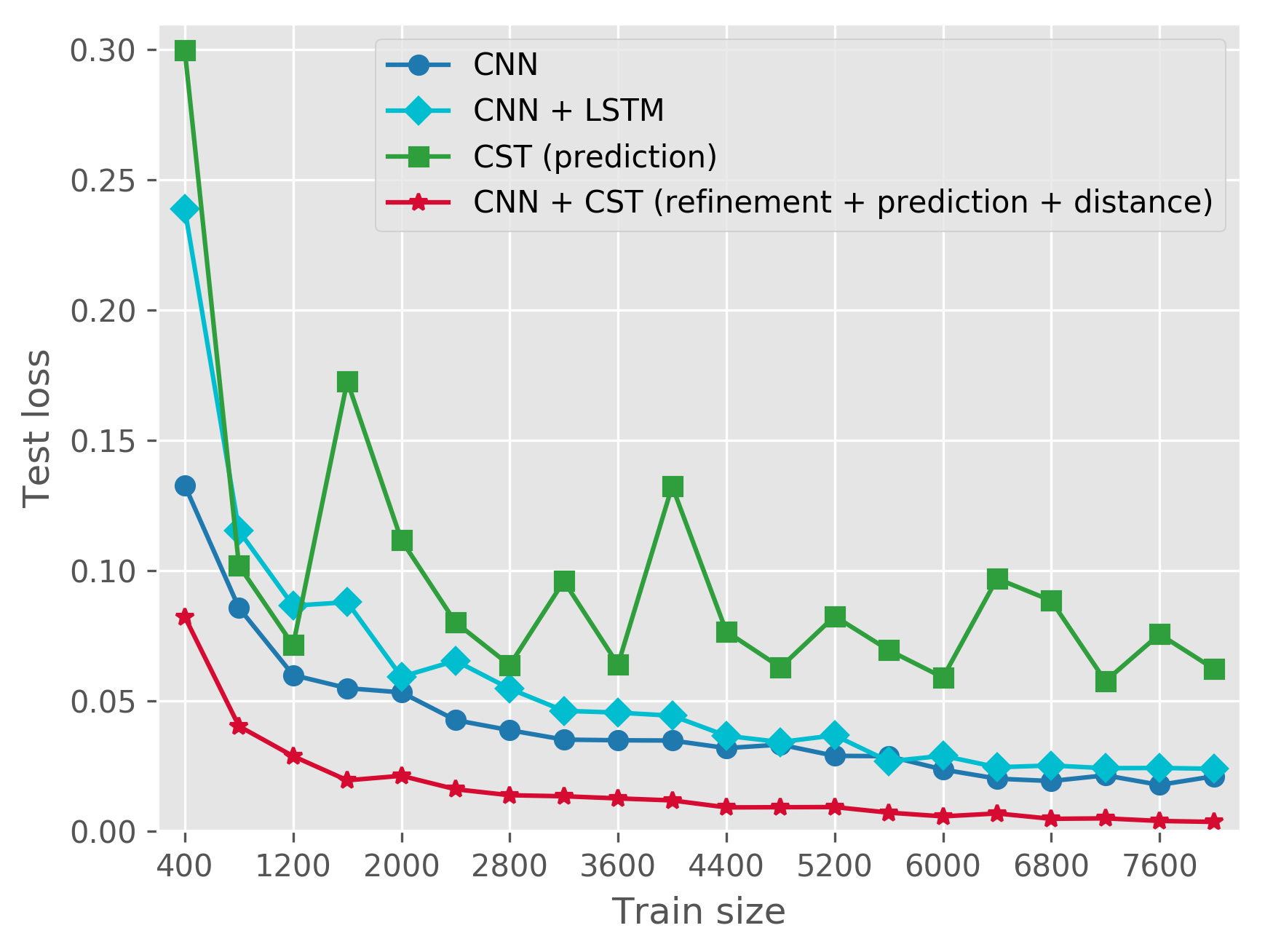
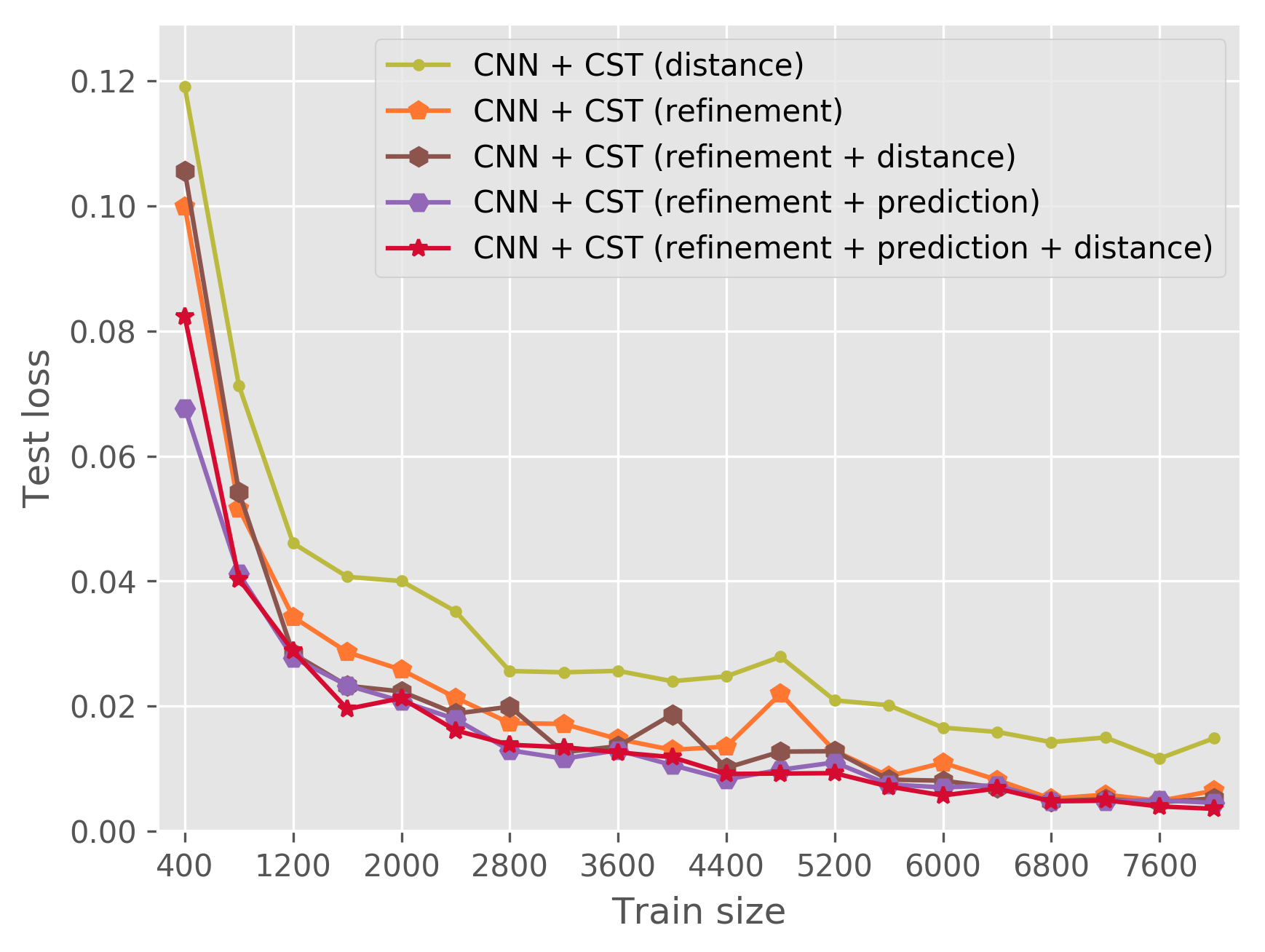
Figure 4: Learning curves for the different setups of our architecture. The plots show how the structural loss (Hamming distance) on the test set changes with increasing size of the training set. On the left, our proposed technique (red curve) is compared against its basic components on their own, namely the CNN (blue curve) and the CST (green curve), and against a CNN+LSTM cascade (light blue curve). On the right, a summary of the contributions of different combinations of features is shown. Best viewed in color.

5.4 The combined model

After training the convolutional network, we combine it with the CST as described in Section 3.

We train the CST model using the structured SVMs method with stochastic subgradient descent (?) for one epoch over the training set. The structured loss used in this task is the Hamming distance between the predicted sequence of symbols and the true sequence.

Figure 4 shows the learning curves resulting from the experiments using the Hamming loss. In the left plot we compare the combined model (CNN + CST) with the single components, i.e., the CNN and the CST in the original variant (?), and the CNN + LSTM cascade. The general trend is rather clear, the CNN has always an edge over the CST, yet their combination always performs better than both. As expected, the gap between the CNN and the combined model is maximal for the smallest dataset, but it remains clearly evident when the curves start to level off (82.9% relative error reduction at the last iteration). The loss of the CNN + LSTM model is overall slightly higher than the one of the CNN model, consistent with what happens for the misclassification error (see Figure 2).

We then computed the breakdown of the CNN + CST results by features of the CST model (see Table 1). When considering distance only, we set its weight $\bm{\mathrm{w}}_{\delta}$ to a negative value, so as to minimize the distance between the prediction of the network and the refined prediction while satisfying the constraints, without any learning on the CST side. We then decomposed the features of the full combined model into: [i] refinement; [ii] refinement + distance; [iii] refinement + prediction. The right plot in Figure 4 shows the learning curves for each of these variants The distance feature is clearly the least effective, even if it already improves over the CNN alone (29.6% relative error reduction at the last iteration). The other features perform quite similarly, but combining all features together achieves the overall best performance.

5.5 Comparison with DeepProbLog

As stated in the introduction, the DeepProbLog framework (?) is capable of combining neural processing with the management of logic and numeric constraints, and can in principle address a recognition task like the one presented here. Indeed, the framework proved capable of learning to add numbers represented as MNIST images (?). The equation recognition task we address here, however, is more complex, as the numbers in the equation have variable length and the position of the operators is not known a-priori. Modelling this problem with DeepProbLog requires the use of non-deterministic predicates, which are extremely expensive. Indeed, we attempted to encode the equation recognition problem in DeepProbLog, but inference turned out to be too memory expensive to be even executed.

6 Related work

Statistical relational learning.

Statistical relational learning (SRL) (?) approaches inject prior knowledge, usually expressed in some logical formalism, into statistical learning models, with a particular emphasis on probabilistic graphical models. In SRL, the logical framework (either propositional or first order logic) is used to define the structure of the data, i.e. the known or likely relationships between the variables, which are then weighted and refined by inductive learning from data. Examples approaches include Relational Bayesian Networks (?), Markov Logic Networks (?), and ProbLog (?). These approaches are not designed for sub-symbolic inputs.

Structured prediction.

Traditional approaches to structured prediction, like conditional random fields (?) and structured output SVMs (?) discriminatively learn an energy or scoring function over candidate input-output pairs based on a joint input-output feature map. Prior knowledge can be injected into these models through propositional (hard and soft) constraints (?; ?; ?). MAP inference is solved using either ad-hoc constrained inference techniques or general solvers for combinatorial or discrete-continuous problems (?; ?; ?). These techniques, however, require one to pre-specify the relevant features (or kernel), which was shown to be suboptimal in many tasks compared to representation learning strategies.

Neural structured prediction.

More recently energy-based structured prediction has been tackled using deep learning models. Notable examples include deep value networks (?), structured prediction energy networks (SPENs) (?) and input convex neural networks (?). These techniques implement the energy function using a neural network and use gradient methods to infer a high-quality candidate output. In contrast to their shallow alternatives, deep structured models do not straightforwardly support the addition of prior knowledge through constraints. The work by Lee et al. (?) addresses this issue without resorting to combinatorial search, by casting the constrained inference of a SPEN into an instance-specific learning problem with a constraint-based loss function. Unlike Nester, this method is not guaranteed to satisfy all the constraints, especially for a complex mix of algebraic and logical ones.

Neuro-symbolic integration.

Effectively combining reasoning with deep networks is still an ongoing research effort. Many attempts have been made to address this issue, most of which focus on forcing the network to learn weights that ultimately produce predictions satisfying the constraints. A popular line of research integrates constraints into the objective function using fuzzy logic, especially the Łukasiewicz T-norm (?; ?; ?). These approaches however cannot guarantee that the predicted outputs satisfy the hard constraints. The same is true for the semantic loss, which encourages the output of a neural network to satisfy given constraints with high probability (?; ?). Furthermore, these approaches are usually restricted to Boolean variables and logical constraints. DeepProbLog (?) extends the ProbLog language (?) with learnable neural predicates. This powerful framework allows to reason about semantic properties of the output variables while using neural networks for low-level inputs. By building on top of a probabilistic programming framework, it inherits its ability to answer probabilistic queries other than MAP inference, something Nester cannot do. On the other hand, DeepProbLog cannot be used to model a complex structured-output prediction problem efficiently, as discussed in our experimental evaluation.

Declarative structured prediction.

Structured learning modulo theories (?) is a structured learning framework dealing with (soft and hard) constraints expressed in a declarative fashion using the SMT formalism and the MiniZinc constraint programming language. The framework has been applied to both passive (?; ?) and interactive learning settings (?). Learning modulo theories shares with Nester the ability to handle hybrid discrete-continuous combinatorial problems. On the other hand its underlying model is a shallow structured SVM and it thus lacks a representation learning component to deal with low-level inputs. Nester can be seen as a neuro-symbolic version of this framework.

Other works.

Some recent approaches have tackled problems at the intersection of constrained optimization and deep learning. For instance, in predict-then-optimize (?) the goal is to predict the parameters of a constrained optimization model (e.g., a scheduling problem) from data, in some cases using a deep neural network (?; ?). In predict-then-optimize, however, the ground-truth value of the parameters to be predicted (for instance, the cost vector of a linear program) is available as supervision, whereas in structured output prediction no supervision is given on the parameters of the constraint program. This makes the two problems conceptually very different. Two other related threads of research are constraint learning (?) and inverse optimization (?; ?), which are also concerned with learning constrained optimization problems from examples. These families of approaches, however, are not tailored for acquiring neuro-symbolic programs and it would be non-trivial to extend them to this purpose.

7 Conclusion

We developed a structured output prediction system combining neural networks and constraint programming, with the aim of jointly leveraging the effectiveness of neural networks in processing raw data with the ability of constraint programming to deal with a wide range of constraints over Boolean and numerical data. The system is conceived for structured prediction tasks where examples are scarce and prior knowledge is abundant. We tested our approach on one such task, namely handwritten equation recognition. A preliminary experiment showed how CNN and even convolutional LSTM, while quickly learning to correct syntactic errors, have serious problems in coping with semantic errors. Our combined approach, in addition to producing consistent predictions by design, is able to improve recognition performance over both the neural network and the constrained structured model on their own, especially with smaller training sets.

We posit that our approach could be applied to several important problems in which prior knowledge is key to their solution, such as dialogue management (?), reinforcement learning in complex environments (?), and interactive recommendation systems (?), all of which we intend to pursue as future work.

References

- Amos, Xu, and Kolter 2017 Amos, B.; Xu, L.; and Kolter, J. 2017. Input convex neural networks. In ICML.
- Bakir et al. 2007 Bakir, G.; Hofmann, T.; Schölkopf, B.; Smola, A.; Taskar, B.; and Vishwanathan, S. 2007. Predicting Structured Data.
- Belanger and McCallum 2016 Belanger, D., and McCallum, A. 2016. Structured prediction energy networks. In ICML.
- Darwiche 2018 Darwiche, A. 2018. Human-level intelligence or animal-like abilities? Communications of the ACM 61(10):56–67.
- Daumé, Langford, and Marcu 2009 Daumé, H.; Langford, J.; and Marcu, D. 2009. Search-based structured prediction. Mach. Learn. 75(3):297–325.
- De Raedt et al. 2020 De Raedt, L.; Dumančić, S.; Manhaeve, R.; and Marra, G. 2020. From Statistical Relational to Neuro-Symbolic Artificial Intelligence. arXiv preprint arXiv:2003.08316.
- De Raedt, Kimmig, and Toivonen 2007 De Raedt, L.; Kimmig, A.; and Toivonen, H. 2007. Problog: A probabilistic prolog and its application in link discovery. In IJCAI, volume 7, 2462–2467. Hyderabad.
- De Raedt, Passerini, and Teso 2018 De Raedt, L.; Passerini, A.; and Teso, S. 2018. Learning constraints from examples. In AAAI.
- Deshwal, Doppa, and Roth 2019 Deshwal, A.; Doppa, J. R.; and Roth, D. 2019. Learning and inference for structured prediction: A unifying perspective. In IJCAI.
- Di Liello et al. 2020 Di Liello, L.; Ardino, P.; Gobbi, J.; Morettin, P.; Teso, S.; and Passerini, A. 2020. Efficient generation of structured objects with constrained adversarial networks. Advances in neural information processing systems.
- Diligenti, Gori, and Scoca 2016 Diligenti, M.; Gori, M.; and Scoca, V. 2016. Learning efficiently in semantic based regularization. In ECML-PKDD.
- Donadello, Serafini, and d’Avila Garcez 2017 Donadello, I.; Serafini, L.; and d’Avila Garcez, A. 2017. Logic tensor networks for semantic image interpretation. In IJCAI.
- Dragone et al. 2018 Dragone, P.; Pellegrini, G.; Vescovi, M.; Tentori, K.; and Passerini, A. 2018. No more ready-made deals: Constructive recommendation for telco service bundling. In Proceedings of the 12th ACM Conference on Recommender Systems, RecSys ’18, 163–171. New York, NY, USA: Association for Computing Machinery.
- Dragone, Teso, and Passerini 2018a Dragone, P.; Teso, S.; and Passerini, A. 2018a. Pyconstruct: Constraint programming meets structured prediction. In IJCAI.
- Dragone, Teso, and Passerini 2018b Dragone, P.; Teso, S.; and Passerini, A. 2018b. Constructive preference elicitation. Frontiers in Robotics and AI 4.
- Elmachtoub and Grigas 2017 Elmachtoub, A. N., and Grigas, P. 2017. Smart “Predict, then Optimize”. arXiv preprint arXiv:1710.08005.
- Erculiani et al. 2018 Erculiani, L.; Dragone, P.; Teso, S.; and Passerini, A. 2018. Automating layout synthesis with constructive preference elicitation. In Joint European Conference on Machine Learning and Knowledge Discovery in Databases.
- Fersini et al. 2014 Fersini, E.; Messina, E.; Felici, G.; and Roth, D. 2014. Soft-constrained inference for named entity recognition. Information Processing & Management.
- Finley and Joachims 2008 Finley, T., and Joachims, T. 2008. Training structural svms when exact inference is intractable. In Proceedings of the 25th International Conference on Machine Learning, 304–311.
- Garnelo, Arulkumaran, and Shanahan 2016 Garnelo, M.; Arulkumaran, K.; and Shanahan, M. 2016. Towards deep symbolic reinforcement learning. arXiv preprint arXiv:1609.05518.
- Getoor and Taskar 2007 Getoor, L., and Taskar, B. 2007. Introduction to statistical relational learning.
- Gygli, Norouzi, and Angelova 2017 Gygli, M.; Norouzi, M.; and Angelova, A. 2017. Deep value networks learn to evaluate and iteratively refine structured outputs. In ICML.
- Hu et al. 2016 Hu, Z.; Ma, X.; Liu, Z.; Hovy, E.; and Xing, E. 2016. Harnessing deep neural networks with logic rules. In ACL.
- Jaeger 1997 Jaeger, M. 1997. Relational bayesian networks. In UAI.
- Joachims et al. 2009 Joachims, T.; Hofmann, T.; Yue, Y.; and Yu, C.-N. 2009. Predicting structured objects with support vector machines. Communications of the ACM 52(11).
- Joachims, Finley, and Yu 2009 Joachims, T.; Finley, T.; and Yu, C. 2009. Cutting-plane training of structural svms. Machine Learning.
- Kingma and Ba 2015 Kingma, D. P., and Ba, J. 2015. Adam: A method for stochastic optimization. In 3rd International Conference on Learning Representations, ICLR.
- Kristjansson et al. 2004 Kristjansson, T.; Culotta, A.; Viola, P.; and McCallum, A. 2004. Interactive information extraction with constrained conditional random fields. In AAAI.
- Lacoste-Julien et al. 2013 Lacoste-Julien, S.; Jaggi, M.; Schmidt, M.; and Pletscher, P. 2013. Block-coordinate frank-wolfe optimization for structural svms. In ICML.
- Lafferty, McCallum, and Pereira 2001 Lafferty, J.; McCallum, A.; and Pereira, F. 2001. Conditional random fields: Probabilistic models for segmenting and labeling sequence data. In ICML.
- Lake et al. 2017 Lake, B.; Ullman, T.; Tenenbaum, J.; and Gershman, S. 2017. Building machines that learn and think like people. Behavioral and Brain Sciences.
- LeCun et al. 2006 LeCun, Y.; Chopra, S.; Hadsell, R.; Huang, F. J.; and et al. 2006. A tutorial on energy-based learning. In Predicting Structured Data. MIT Press.
- Lee et al. 2017 Lee, J.; Wick, M.; Tristan, J.; and Carbonell, J. 2017. Enforcing output constraints via sgd: A step towards neural lagrangian relaxation. In NIPS.
- Lison 2015 Lison, P. 2015. A hybrid approach to dialogue management based on probabilistic rules. Computer Speech & Language.
- Mandi and Guns 2020 Mandi, J., and Guns, T. 2020. Interior Point Solving for LP-based prediction+ optimisation. In NeurIPS.
- Mandi et al. 2020 Mandi, J.; Stuckey, P. J.; Guns, T.; et al. 2020. Smart predict-and-optimize for hard combinatorial optimization problems. In AAAI, volume 34.
- Manhaeve et al. 2018 Manhaeve, R.; Dumančić, S.; Kimmig, A.; Demeester, T.; and De Raedt, L. 2018. DeepProblog: Neural probabilistic logic programming. In NeurIPS.
- Nethercote et al. 2007 Nethercote, N.; Stuckey, P.; Becket, R.; Brand, S.; Duck, G.; and Tack, G. 2007. Minizinc: Towards a standard cp modelling language. In CP.
- Otter, Medina, and Kalita 2021 Otter, D. W.; Medina, J. R.; and Kalita, J. K. 2021. A survey of the usages of deep learning for natural language processing. IEEE Trans. Neural Networks Learn. Syst. 32(2):604–624.
- Ratliff, Bagnell, and Zinkevich 2007 Ratliff, N.; Bagnell, J.; and Zinkevich, M. 2007. (approximate) subgradient methods for structured prediction. In AISTATS.
- Richardson and Domingos 2006 Richardson, M., and Domingos, P. 2006. Markov logic networks. Machine learning.
- Ross, Gordon, and Bagnell 2011 Ross, S.; Gordon, G.; and Bagnell, D. 2011. A reduction of imitation learning and structured prediction to no-regret online learning. In Proceedings of the Fourteenth International Conference on Artificial Intelligence and Statistics, 627–635.
- Roth and Yih 2005 Roth, D., and Yih, W. 2005. Integer linear programming inference for conditional random fields. In ICML.
- Santoro et al. 2017 Santoro, A.; Raposo, D.; Barrett, D.; Malinowski, M.; Pascanu, R.; Battaglia, P.; and Lillicrap, T. 2017. A simple neural network module for relational reasoning. In NIPS.
- Tan, Delong, and Terekhov 2019 Tan, Y.; Delong, A.; and Terekhov, D. 2019. Deep inverse optimization. In International Conference on Integration of Constraint Programming, Artificial Intelligence, and Operations Research.
- Tan, Terekhov, and Delong 2020 Tan, Y.; Terekhov, D.; and Delong, A. 2020. Learning linear programs from optimal decisions. In NeurIPS.
- Teso, Sebastiani, and Passerini 2017 Teso, S.; Sebastiani, R.; and Passerini, A. 2017. Structured learning modulo theories. Artificial Intelligence 244.
- Tsochantaridis et al. 2004 Tsochantaridis, I.; Hofmann, T.; Joachims, T.; and Altun, Y. 2004. Support vector machine learning for interdependent and structured output spaces. In ICML.
- Xu et al. 2017 Xu, J.; Zhang, Z.; Friedman, T.; Liang, Y.; and Van den Broeck, G. 2017. A semantic loss function for deep learning with symbolic knowledge. In ICML.
- Zambaldi et al. 2018 Zambaldi, V.; Raposo, D.; Santoro, A.; Bapst, V.; Li, Y.; Babuschkin, I.; Tuyls, K.; Reichert, D.; Lillicrap, T.; and Lockhart, E. 2018. Relational deep reinforcement learning. arXiv preprint arXiv:1806.01830.