[2103.17229] Joint Deep Multi-Graph Matching and 3D Geometry Learning from Inhomogeneous 2D Image Collections

1 Graph for non-learning based methods

As the nodes are the key points in images, we need to construct the edges for each graph. Each edge $(k,l)\in\mathcal{E}_{j}$ requires two features $w_{kl}$ and $\theta_{kl}$ , where $w_{kl}$ is the pairwise distance between the connected nodes $v_{k}$ and $v_{l}$ , and $\theta_{kl}$ is the absolute angle between the edge and the horizontal line with $0\leq\theta_{kl}\leq\pi/2$ . The edge affinity between edges $(k,l)$ in $\mathcal{G}_{1}$ and $(a,b)$ in $\mathcal{G}_{2}$ is computed as $e_{(k,a),(l,b)}=\text{exp}(-(|w_{kl}-w_{ab}|+|\theta_{kl}-\theta_{ab}|)/2)$ . The edge affinity can overcome the ambiguity of orientation because objects in real-world datasets typically have a natural up direction (e.g. people/animals stand on their feet, car/bikes on their tyres).

	aero	bike	bird	boat	bottle	bus	car	cat	chair	cow	table	dog	horse	mbike	person	plant	sheep	sofa	train	tv	Avg.
PCA	40.92	15.48	44.91	45.30	14.55	41.83	55.97	42.97	35.99	44.30	41.59	49.10	43.68	33.33	35.04	24.67	53.93	45.87	44.00	29.39	39.19
CSGM	49.08	51.50	60.13	67.84	81.13	80.36	67.40	57.10	51.26	61.42	56.16	55.28	61.61	54.17	54.57	96.84	60.71	58.30	96.6	93.60	65.75
Ours	100	100	100	100	100	100	100	100	100	100	100	100	100	100	100	100	100	100	100	100	100

Table 1: Cycle consistency scores (in percent) of PCA (wang2019PCA), CSGM (wang2020combinatorial) and ours on the Pascal VOC Keypoints dataset. Our method is the only one that guarantees cycle consistency for all categories.

Figure 1: The average matching accuracy and cycle consistency score of PCA (wang2019PCA), CSGM (wang2020combinatorial) and ours on Pascal VOC dataset.

2 Cycle Consistency

We further provide quantitative evaluations of the cycle consistency on the Pascal VOC dataset, as shown in Table 1. We quantify in terms of the cycle consistency score, which is computed as follows:

1.

Given three graphs $\{\mathcal{G}_{j}\}$ , $\{\mathcal{G}_{k}\}$ and $\{\mathcal{G}_{l}\}$ , we use the trained network to predict $X_{jk}$ , $X_{jl}$ and $X_{kl}$ .
2.

We compute the composed pairwise matching between $\{\mathcal{G}_{k}\}$ and $\{\mathcal{G}_{l}\}$ by $X^{\prime}_{kl}=X_{jk}^{T}X_{jl}$ .
3.

We denote the number of points that $X^{\prime}_{kl}$ equals to $X_{kl}$ as $m_{\text{cycle}}$ and the number of points in $X_{kl}$ as $m_{kl}$ . The cycle consistency score is then computed as

$\text{cycle consistency score}=100\times\frac{m_{\text{cycle}}}{m_{kl}}\%.$ (1)

Note that in this case, we only consider the common points that are observed in $\{\mathcal{G}_{j}\}$ , $\{\mathcal{G}_{k}\}$ and $\{\mathcal{G}_{l}\}$ .

In Fig. 1, we show the average matching accuracy and cycle consistency score of our method and compare it with PCA (wang2019PCA) and CSGM (wang2020combinatorial). It is clear that our method can achieve comparable accuracy and the best cycle consistency at the same time.

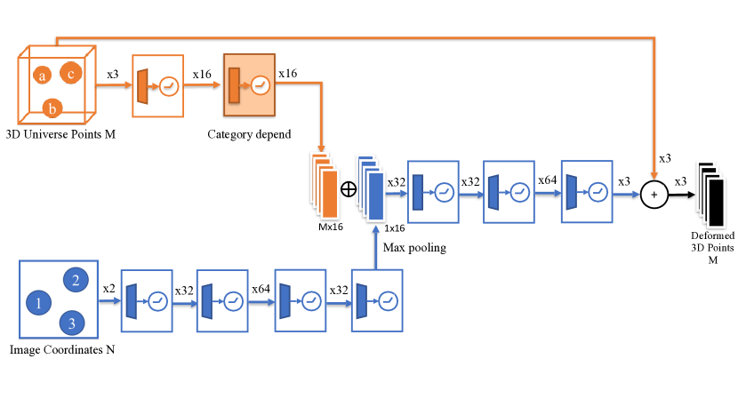
Refer to caption — Figure 2: The detailed architecture of the deformation module. Each box contains a linear layer and a ReLU unit. The linear layer in dashed box on 3D universe points is determined by the category of the input object. The goal of this layer is to alert the neural network about deformations in various categories.

3 Network architecture

We show the architecture of the deformation module in Fig. 2. Each linear layer is followed by a Rectified Linear Unit (ReLU). Additionally, we introduce a linear layer depending on the category of the input object. Its purpose is to assist the neural network in distinguishing between different deformations among categories. For detailed information on Graph Matching Network, readers are referred to (wang2020combinatorial)

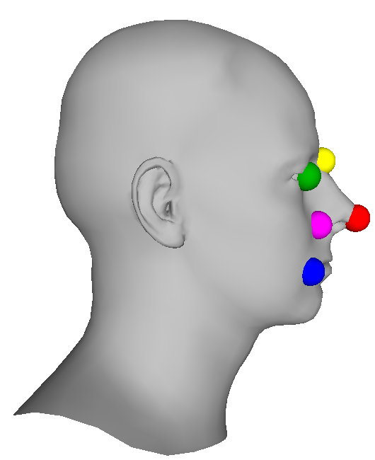
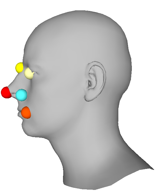
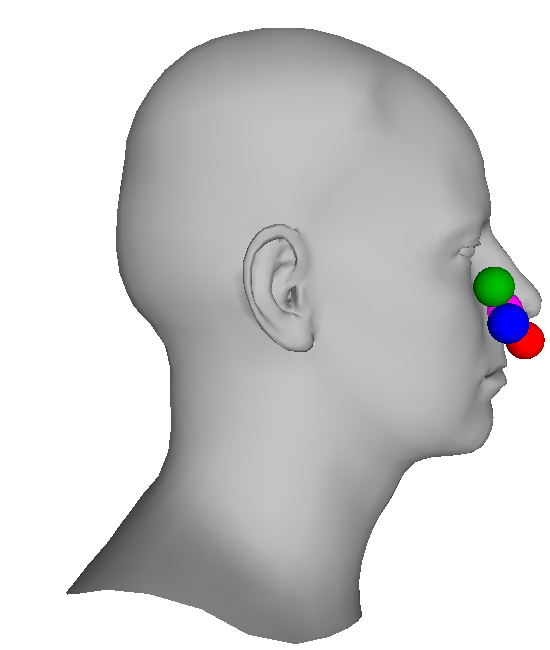
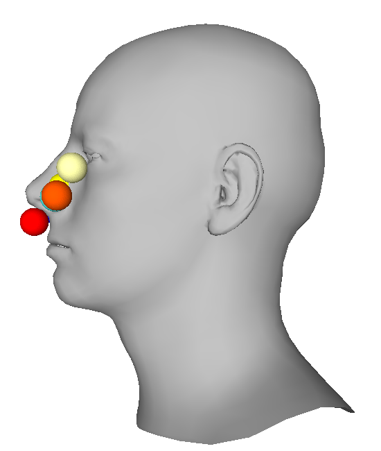
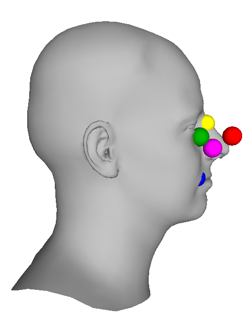
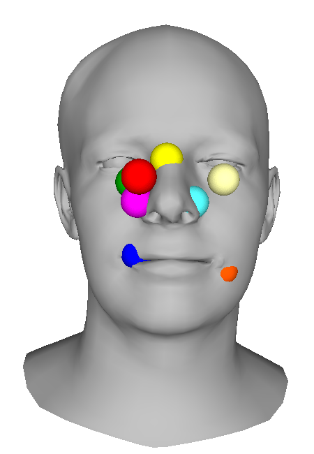
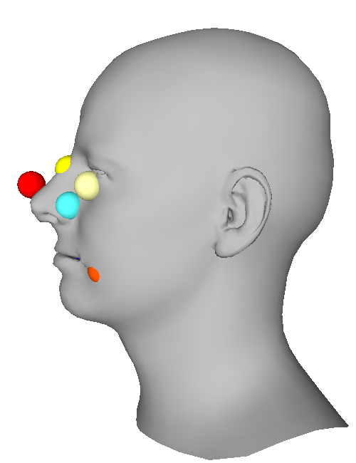
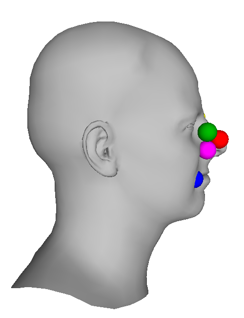
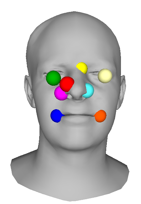
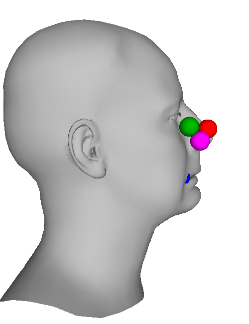
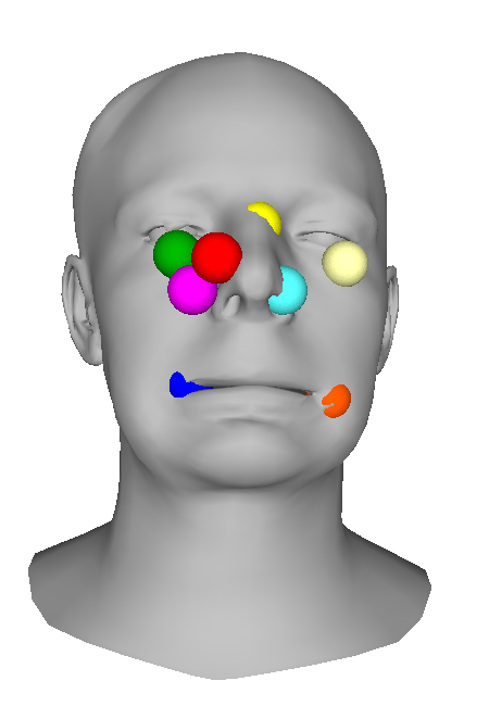
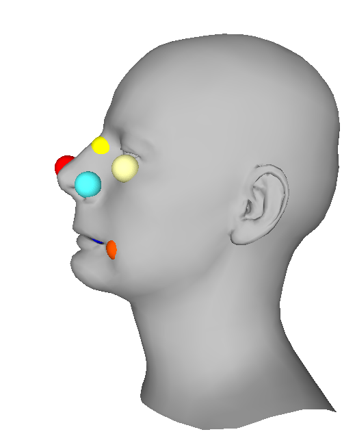
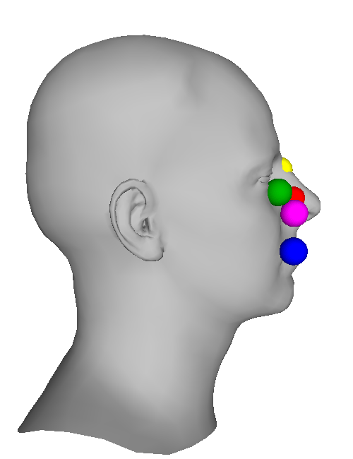
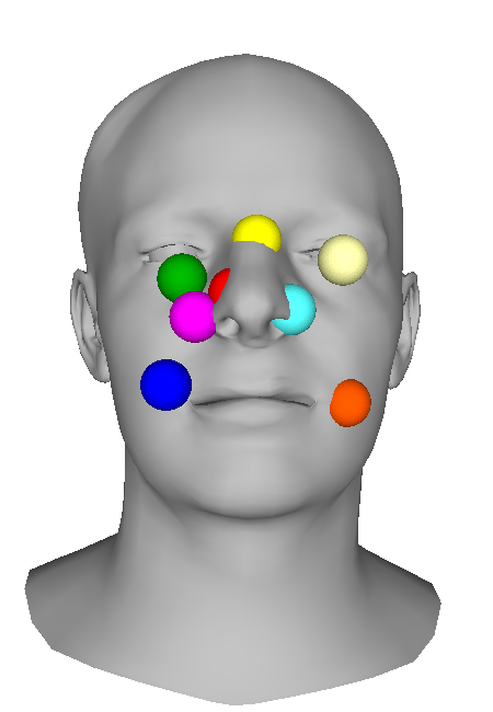
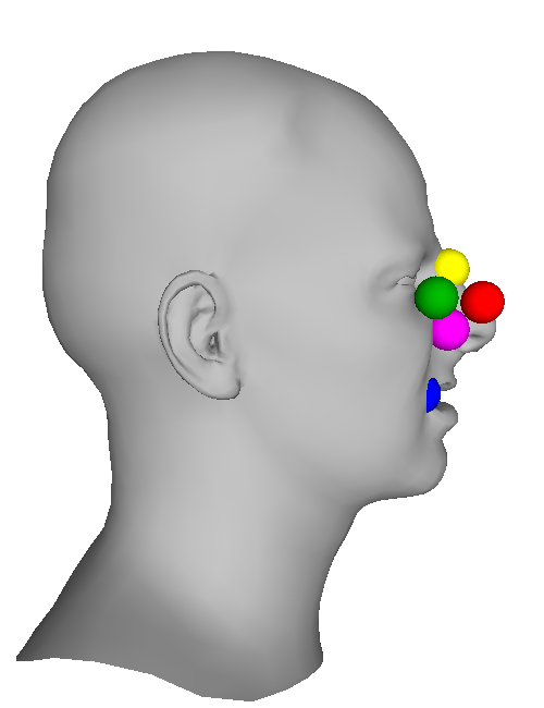
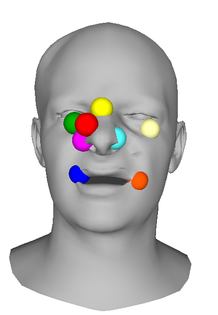
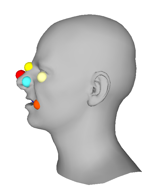
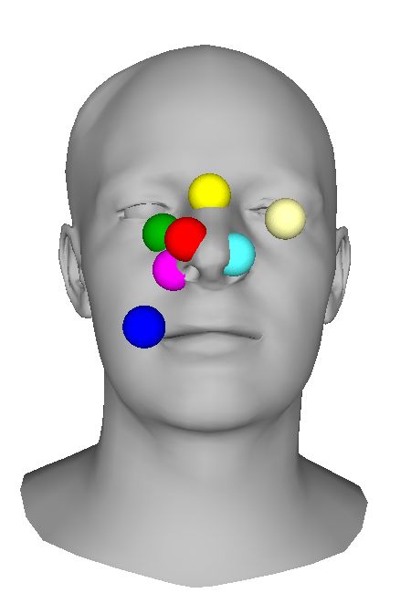
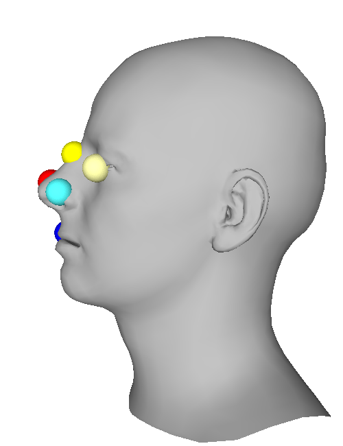
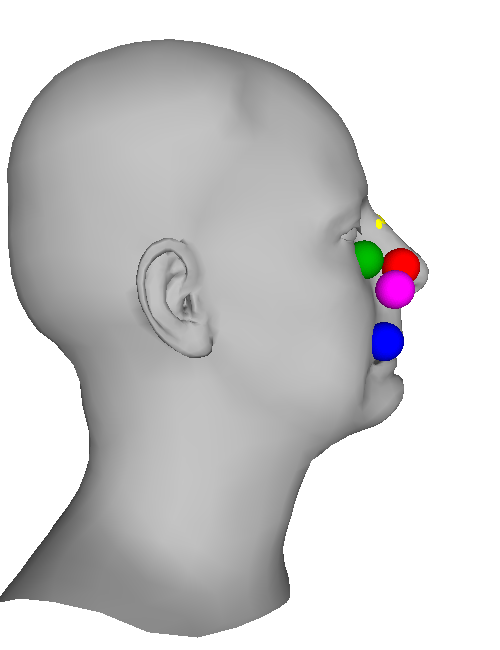
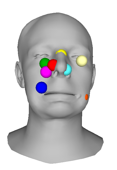
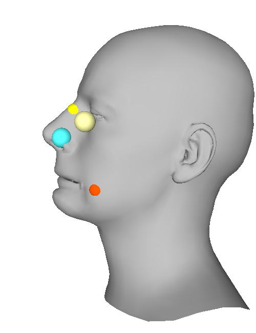
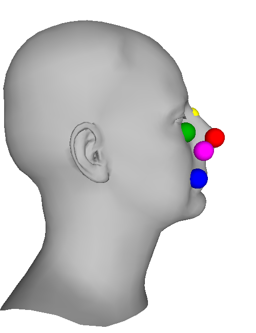
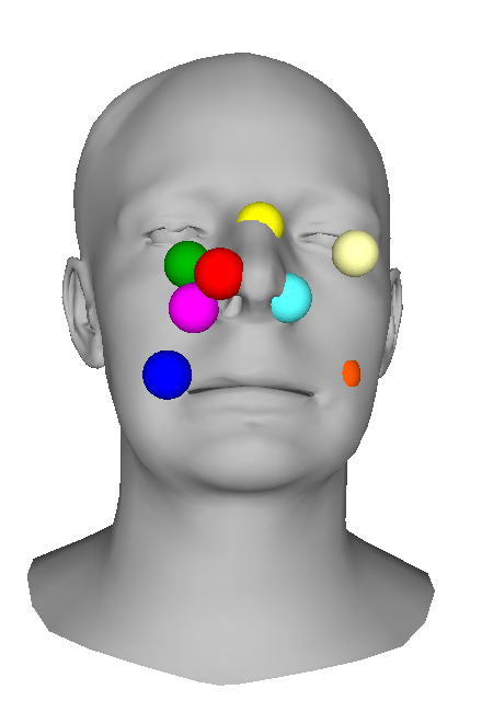
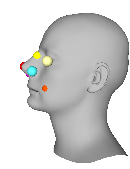
4 More Deformation Results

We provide more qualitative results for our deformation module, see Fig. 3. As shown in the figure, the deformation module is able to refine the 3D universe points. Although 3D reconstructions are not perfect, we can observe that they represent the overall 3D structure well, and are thus valuable for matching respective key points.