Logical Abstractions for Noisy Variational
Quantum Algorithm Simulation

Abstract.

Due to the unreliability and limited capacity of existing quantum computer prototypes, quantum circuit simulation continues to be a vital tool for validating next generation quantum computers and for studying variational quantum algorithms, which are among the leading candidates for useful quantum computation. Existing quantum circuit simulators do not address the common traits of variational algorithms, namely: 1) their ability to work with noisy qubits and operations, 2) their repeated execution of the same circuits but with different parameters, and 3) the fact that they sample from circuit final wavefunctions to drive a classical optimization routine. We present a quantum circuit simulation toolchain based on logical abstractions targeted for simulating variational algorithms. Our proposed toolchain encodes quantum amplitudes and noise probabilities in a probabilistic graphical model, and it compiles the circuits to logical formulas that support efficient repeated simulation of and sampling from quantum circuits for different parameters. Compared to state-of-the-art state vector and density matrix quantum circuit simulators, our simulation approach offers greater performance when sampling from noisy circuits with at least eight to 20 qubits and with around 12 operations on each qubit, making the approach ideal for simulating near-term variational quantum algorithms. And for simulating noise-free shallow quantum circuits with 32 qubits, our simulation approach offers a $66\times$ reduction in sampling cost versus quantum circuit simulation techniques based on tensor network contraction.

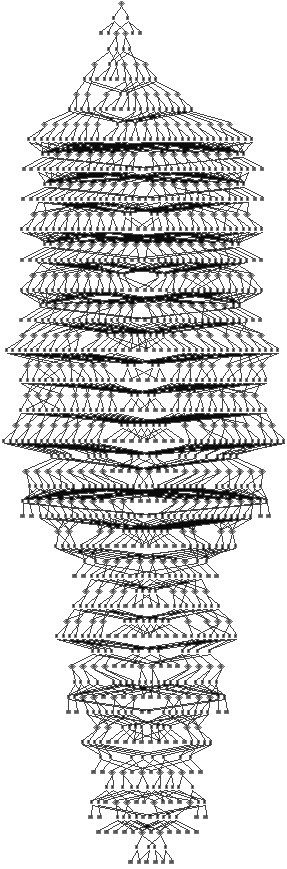
Before

After

Figure 1. Equivalent knowledge compilation representations of a 4-qubit noisy QAOA quantum circuit. In this work we calculate and sample amplitudes from arithmetic circuits (ACs) representing noisy quantum circuits. To the left, direct compilation results in ACs where qubit states ordered in time progresses from top to bottom. Above, optimizations such as logical minimization, qubit state reordering, and eliding internal qubit states reduce the size of the AC. The reduced but equivalent representation leads to more efficient simulation and sampling.

1. Introduction

Consensus among quantum systems researchers is that variational algorithms are among the most important near-term applications of quantum computing (Preskill, 2018; National Academies of Sciences, Engineering, and Medicine, 2019). Variational algorithms work by using a classical computer to train for optimal parameters that minimize a function evaluated by a quantum computer. Examples include the quantum approximate optimization algorithm (QAOA) (Farhi et al., 2014; Farhi and Harrow, 2016) and the variational quantum eigensolver (VQE) (Peruzzo et al., 2014) algorithm for physical simulations. Unlike prominent quantum algorithms such as Shor’s factoring (Shor, 1997) and Grover’s search (Grover, 1996) algorithms, variational algorithms can extract useful computation out of noisy intermediate-scale quantum (NISQ) computer prototypes, which only support unreliable operations on a limited number of qubits (the fundamental unit of quantum computing).

A further consequence of the limited capacity, reliability, and endurance of existing quantum prototypes is that simulation using classical computers continues to be a critical research tool (National Academies of Sciences, Engineering, and Medicine, 2019, Chapter 6.3). Classical computer simulations of quantum algorithm circuits are important for developing new quantum algorithms and for validating results from quantum prototypes.

Thus far, the most advanced quantum circuit simulators are not geared for simulating important variational quantum algorithms. Quantum computing research would benefit from a simulator that supports variational algorithms specifically, which would require a simulator that 1) supports simulating the effect of noise, 2) efficiently supports repeated simulations with different parameters, 3) offers an ability to sample from the output of the quantum computer, and 4) excels at simulating quantum circuits with many qubits and relatively few operations per qubit. Unfortunately, leading quantum circuit simulators have instead focused on simulations that establish the point at which limitations of classical computing give way to quantum computers having an advantage, a milestone termed quantum supremacy (Arute et al., 2019; Harrow and Montanaro, 2017; Markov et al., 2018; Terhal, 2018). Such simulators can only simulate quantum circuits that are ideal (noise-free), and they cannot reuse computation results across simulation runs. The clear mismatch between the requirements for variational algorithm versus supremacy simulations have resulted in simulators that do not adequately support important variational workloads.

The key insight of our paper is that knowledge compilation—a technique for efficient repeated inference originating in artificial intelligence research (Darwiche, 2009; Darwiche and Marquis, 2002)—can serve as the basis for a quantum circuit simulation toolchain geared for variational algorithms. In a knowledge compilation approach to performing inference, knowledge about probabilistic relationships between events is first encoded in a graphical model such as a Bayesian network (Darwiche, 2009; Koller and Friedman, 2009; Pearl, 2014). The knowledge compilation techniques convert Bayesian networks into minimized representations of logical formulas called arithmetic circuits (ACs, Figure 1) that enable repeated inference and sampling queries with different parameters and new choices for inference outcomes (Chavira and Darwiche, 2008). These features of the knowledge compilation approach—namely, 1) the ability to represent and manipulate probabilistic information, 2) the ability to compile probabilistic model structural information into minimized formats, 3) the ability to efficiently sample from the same model but for varying parameters and evidence—match well with the requirements for variational quantum algorithm simulation.

We built a toolchain to test this idea of using knowledge compilation for variational algorithms quantum circuit simulation. Our toolchain consists of:

1. A front-end for converting noisy quantum circuits (specified in Google’s Cirq framework) to complex-valued Bayesian networks (Biamonte and Bergholm, 2017; Boixo et al., 2017; Markov and Shi, 2008; Pienaar and Brukner, 2015; Tucci, 1995; Yeang, 2010), which we extend to correctly encode quantum noise mixtures and channels. Compared to conventional quantum circuits where complex-valued quantum amplitudes and real-valued noise probabilities are treated separately, the Bayesian network encoding unifies quantum states and noise events in a single representation.

2. A compiler that converts Bayesian networks representing noisy quantum circuits into conjunctive normal form (CNF) logic formulas. The CNFs encode the quantum circuits’ structural information: the sets of logic variable assignments that satisfy the CNF correspond to all sets of qubit state assignments that are consistent with the original quantum circuit’s semantics. This structural information can be reused across simulations independently of quantum amplitude and noise probability parameters, which vary across simulations, which is a key benefit over prior simulation techniques.

3. A compiler that converts CNFs to ACs. An AC enumerates and assigns a weight value to each set of variable assignments that satisfy a logical formula (Darwiche, 2009). Summing the weights across all qubit state assignments results in the output amplitudes that we seek to find in the quantum circuit simulation task. The compiler can factor away the variables that represent intermediate qubit states, thereby enabling the quantum circuit simulator to find the probability amplitude for an outcome without incurring the cost of finding the amplitudes of intermediate qubit states. The ACs also enable a Markov chain Monte Carlo procedure for sampling sets of qubit outcomes according to their measurement probability.

We validate our compilation and simulation approach for both noise-free and noisy quantum circuits, demonstrating correct results for a suite of quantum algorithms including Deutsch-Jozsa, Bernstein-Vazirani, hidden shift, quantum Fourier transform, Shor’s, and Grover’s algorithms.

We benchmark the performance of our simulator for sampling outputs for a QAOA algorithm for Max-Cut and a VQE algorithm for finding the minimum energy configuration of a 2D Ising model. Compared to state-of-the-art simulators for both ideal and noisy quantum circuits, our simulator excels at sampling from circuits with at least eight to 20 qubits and with around 12 operations per qubit—a range of qubit counts and operations that includes many meaningful variational algorithm problems. And for simulating ideal shallow quantum circuits with 32 qubits, our simulation approach offers a $66\times$ reduction in sampling cost versus simulators based on tensor network contraction. The advantages are due to the more compact representation, the circuit minimization and memoization capabilities of our approach, and due to the storage costs for conventional simulators based on matrix representations. The improved simulation performance facilitates studying variational algorithms and validating prototype quantum computer results in the NISQ era of quantum computing.

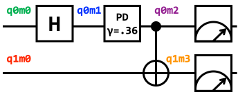
(a) Noisy quantum circuit for creating a Bell state consisting of two entangled qubits. The circuit comprises two qubits, q0 and q1, initialized to initial quantum states q0m0 and q1m0 respectively. The noise model in this quantum circuit is a phase damping (PD) noise channel with a probability of happening $\gamma=36\%$ of the time. Following a Hadamard (H) gate and the noise event, qubit q0 has states q0m1 and q0m2 respectively. Following a CNOT gate qubit q1 has state q1m3.

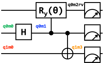
(b) A transformed quantum circuit equivalent to the one to the left. The phase damping channel is replaced by an equivalent controlled rotation—$\theta=\mathrm{arcsin}(\sqrt{\gamma})$ about the y-axis—and a measurement on an ancillary qubit (Nielsen and Chuang, 2011, Page 385). The measurement outcome on the ancillary qubit represents whether or not the noise event takes place. The fact that noise channels can be thought of as spurious measurements makes them difficult to simulate compared to noise mixtures.

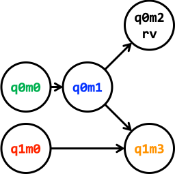
(c) Bayesian network representation of the noisy Bell state quantum circuit in the left two subfigures. The node q0m2rv represents the possible noise events associated with the phase damping noise channel. Each node has an associated conditional amplitude table shown in Tables 5(a), 5(b), and 5(c). The directed edges represent dependencies between qubit states.

Figure 2. Noisy Bell state quantum circuit and its Bayesian network representation.

2. Background on Quantum Circuit Simulation and Variational Algorithms

We summarize necessary background on the representation of noise-free and noisy quantum states, on simulating quantum circuits, and on variational quantum algorithms.

2.1. Ideal Quantum Circuit Simulation

Quantum circuit simulation entails using a classical computer to calculate the outputs of a quantum computer. Quantum circuit simulation is useful for discovering new quantum algorithms, validating the execution of quantum programs on unreliable quantum hardware (Arute et al., 2019; Cross et al., 2019; Resch and Karpuzcu, 2019; Huang and Martonosi, 2019a, b), and understanding the limitations of classical and quantum computation (Arute et al., 2019; Harrow and Montanaro, 2017; Markov et al., 2018; Terhal, 2018). To understand quantum circuit simulation, first we have to understand the representation of quantum states and operations.

2.1.1. The State Vector Representation for Quantum Pure States

The fundamental unit of computation in a quantum computer is a qubit. A single qubit has a state represented by the vector $\alpha\ket{0}+\beta\ket{1}=\begin{bmatrix}\alpha,\beta\end{bmatrix}^{\intercal}$, where $\ket{0}$ and $\ket{1}$ are orthonormal standard basis vectors and $\alpha$ and $\beta$ are complex-valued amplitudes. It is required that $|\alpha|^{2}+|\beta|^{2}=1$. The state of $N$ qubits is represented by a state vector that has size $2^{N}$. For example, two qubits have a state represented by the vector $\alpha\ket{00}+\beta\ket{01}+\gamma\ket{10}+\delta\ket{11}=\begin{bmatrix}\alpha,\beta,\gamma,\delta\end{bmatrix}^{\intercal}$, where again $|\alpha|^{2}+|\beta|^{2}+|\gamma|^{2}+|\delta|^{2}=1$.

Using Figure 2(a) as an example, if qubit state ${\color[rgb]{0,1,0}\texttt{q0m0}}=\ket{0}$ and ${\color[rgb]{1,0,0}\texttt{q1m0}}=\ket{0}$, then the state vector of the two qubits is found using the tensor product (denoted $\otimes$):

$${\color[rgb]{0,1,0}\texttt{q0m0}}\otimes{\color[rgb]{1,0,0}\texttt{q1m0}}=\ket{0}\otimes\ket{0}=\begin{bmatrix}1\\ 0\end{bmatrix}\otimes\begin{bmatrix}1\\ 0\end{bmatrix}=\begin{bmatrix}1\\ 0\\ 0\\ 0\end{bmatrix}=\ket{00}$$

2.1.2. The Unitary Matrix Representation of Quantum Gates and Circuits

Quantum computation proceeds by applying quantum gates on quantum states encoded on qubits. Quantum gates are represented by norm-preserving unitary matrices, that is, matrices that ensure that the sums of squares of amplitudes remain 1. For example one important quantum gate is the Hadamard gate which has a unitary matrix representation of:

$$H=\begin{bmatrix}\frac{1}{\sqrt{2}}&\frac{1}{\sqrt{2}}\\ \frac{1}{\sqrt{2}}&-\frac{1}{\sqrt{2}}\end{bmatrix}$$

When quantum gates act on pure states, the resulting state is found via matrix vector multiplication of unitary matrices and state vectors. Using Figure 2(a) as an example, the qubit state q0m1 after the Hadamard gate is:

(1) $${\color[rgb]{0,0,1}\texttt{q0m1}}=H{\color[rgb]{0,1,0}\texttt{q0m0}}=\begin{bmatrix}\frac{1}{\sqrt{2}}&\frac{1}{\sqrt{2}}\\ \frac{1}{\sqrt{2}}&-\frac{1}{\sqrt{2}}\end{bmatrix}\begin{bmatrix}1\\ 0\end{bmatrix}=\begin{bmatrix}\frac{1}{\sqrt{2}}\\ \frac{1}{\sqrt{2}}\end{bmatrix}=\frac{1}{\sqrt{2}}\ket{0}+\frac{1}{\sqrt{2}}\ket{1}$$

2.2. Noisy Quantum Circuit Simulation

In contrast to simulating noise-free ideal quantum circuits, simulating realistic quantum circuits requires the ability to represent noisy quantum mixed states and the ability to model various non-ideal effects. Existing prototype quantum computers are unreliable due to various non-ideal effects. The effects include environmental disturbance of delicate quantum states leading to decoherence, imprecise application of operations, and measurement error. The outcome of quantum states in a noisy quantum circuit varies depending on whether noise events takes place, so a greater amount of information is needed to account for all the possibilities, thereby making the task of simulating noisy circuits harder than simulating ideal ones. To understand this challenge we introduce the representation of noisy quantum states and models of quantum noise.

2.2.1. The Density Matrix Representation of Quantum Mixed States

Density matrices represent noisy quantum states as probabilistic ensembles of pure states. A density matrix $\rho$ for pure states $\ket{\psi}$ has the form: $\rho=\sum_{j}p_{j}\ket{\psi_{j}}\bra{\psi_{j}}$, where $p_{j}$ is the probability that the mixed state is the pure state $\ket{\psi_{j}}$, $\bra{\psi_{j}}$ is the conjugate transpose of $\ket{\psi_{j}}$, and $\sum_{j}p_{j}=1$. Using Figure 2(a) as an example, we may wish to have a density matrix representation of q0m1 in preparation for calculating the effect of quantum noise on that qubit state. The density matrix representation of q0m1 from Equation 1 is:

(2) $$\begin{split}\rho_{{\color[rgb]{0,0,1}\texttt{q0m1}}}&=\Big{(}\frac{1}{\sqrt{2}}\ket{0}+\frac{1}{\sqrt{2}}\ket{1}\Big{)}\Big{(}\frac{1}{\sqrt{2}}\bra{0}+\frac{1}{\sqrt{2}}\bra{1}\Big{)}\\ &=\begin{bmatrix}\frac{1}{\sqrt{2}}\\ \frac{1}{\sqrt{2}}\end{bmatrix}\begin{bmatrix}\frac{1}{\sqrt{2}}&\frac{1}{\sqrt{2}}\end{bmatrix}=\begin{bmatrix}\frac{1}{2}&\frac{1}{2}\\ \frac{1}{2}&\frac{1}{2}\end{bmatrix}\end{split}$$

2.2.2. The Kraus Operator Representation of Quantum Noise Channels

Table 1. Summary of canonical quantum noise models.

		Quantum noise mixtures	Quantum noise channels
Noise effects	Pauli-X type	Bit flip noise	Amplitude damping noise (related to T1 time)
	Pauli-Z type	Phase flip noise	Phase damping noise (related to T2 time)
	Combinations	Symmetric / asymmetric depolarizing noise	Generalized amplitude damping
Sim. technique		Can model as probabilistic ensembles of state vectors	Requires density matrix representation

Quantum noise can be modeled as a quantum noise channel $\mathcal{E}$, which acts on a quantum mixed state $\rho$ to create a new mixed state: $\mathcal{E}(\rho)=\sum_{k}E_{k}\rho E_{k}^{\intercal}$, where the Kraus operators $E$ represent different effects on the quantum state due to the noise channel.

Important noise channel types are listed in Table 1 (Nielsen and Chuang, 2011, Chapter 8.3). The table shows that noise models can be classified along several dimensions. The first dimension is in the type of effect the noise has on the quantum state: Pauli-X type noises disturb the quantum basis state, while Pauli-Z type noises disturb the phase. There are also combinations of these types of noise. The second dimension of classification is in terms of whether density matrices are needed to model the noisy states. In this work we consider all of these types of noise.

For example, one type of quantum noise channel is phase damping noise, which has the Kraus operators:

$$E_{0}=\begin{bmatrix}1&0\\ 0&\sqrt{1-\gamma}\end{bmatrix},\qquad E_{1}=\begin{bmatrix}0&0\\ 0&\sqrt{\gamma}\end{bmatrix}$$

where $\gamma$ is a probability parameter describing the strength of the noise channel. Using Figure 2(a) as an example, the density matrix representation of qubit state q0m2 after a phase damping channel (with $\gamma=.36$) acts on q0m1 from Equation 2 is:

$$\rho_{{\color[rgb]{.5,0,.5}\texttt{q0m2}}}=\mathcal{E}(\rho_{{\color[rgb]{0,0,1}\texttt{q0m1}}})=\begin{bmatrix}\frac{1}{2}&\frac{0.8}{2}\\ \frac{0.8}{2}&\frac{1}{2}\end{bmatrix}$$

Finally, the two-qubit CNOT gate has a unitary matrix representation of:

$$CNOT=\begin{bmatrix}1&0&0&0\\ 0&1&0&0\\ 0&0&0&1\\ 0&0&1&0\\ \end{bmatrix}$$

such that the final density matrix is:

(3) $$\begin{split}\rho_{{\color[rgb]{.5,0,.5}\texttt{q0m2}}}\otimes\rho_{{\color[rgb]{1,.5,0}\texttt{q1m3}}}&=CNOT(\rho_{{\color[rgb]{.5,0,.5}\texttt{q0m2}}}\otimes\rho_{{\color[rgb]{1,0,0}\texttt{q1m0}}})CNOT^{\intercal}\\ &=\begin{bmatrix}\frac{1}{2}&0&0&\frac{0.8}{2}\\ 0&0&0&0\\ 0&0&0&0\\ \frac{0.8}{2}&0&0&\frac{1}{2}\\ \end{bmatrix}\end{split}$$

Outside of these canonical quantum noise mixture and channel models, other types of operational error—such as imprecise gate operations and measurement error—can be modeled as one of the canonical noise models in conjunction with an otherwise ideal operation or measurement.

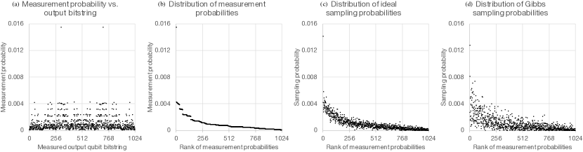
Figure 3. The probability distribution for output qubit measurements in variational quantum algorithms is sharply peaked. A few qubit bitstrings dominate the output probability distribution for this 10-qubit quantum circuit performing QAOA for Max-Cut. Since a few bitstrings dominate the outcomes, sampling the outcomes is more efficient than finding the full probability distribution.

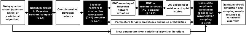
Figure 4. Toolchain for noisy quantum algorithm simulation via knowledge compilation of probabilistic program representations.

2.3. Near-Term Variational Quantum Algorithms as Target Simulation Workload

We focus on quantum circuit simulation for algorithms that are candidates for near-term useful quantum computation. Such algorithms are designed to run on near-term noisy, intermediate-scale quantum (NISQ) computers (Anschuetz et al., 2019; Bravo-Prieto et al., 2019; Huang et al., 2019; Lubasch et al., 2020; National Academies of Sciences, Engineering, and Medicine, 2019; Preskill, 2018). Specifically, we evaluate our simulation approach on two representative NISQ algorithms: one is a quantum approximate optimization algorithm (QAOA) for Max-Cut (Arute et al., 2020; Farhi et al., 2014; Farhi and Harrow, 2016; Szegedy, 2019), and the other is a variational quantum eigensolver (VQE) for an Ising model physics simulation (Barahona, 1982; Peruzzo et al., 2014).

These hybrid quantum-classical algorithms rely on a classical computer running an optimization routine such as the Nelder-Mead method to find optimal parameters for a quantum circuit. The quantum computer serves only to find an objective function from the system under study to guide the overall optimization loop. The quantum circuit parameters that minimize the objective function encode the desired algorithm results.

The quantum circuits involved in these important variational algorithms have distinct traits, and so simulating these circuits is also a distinct challenge. Compared to the quantum circuits involved in other algorithms, variational quantum algorithms:

1. do not rely on error-corrected ideal qubits and operations, and are therefore sensitive to the reliability and noise characteristics of the underlying hardware;

2. require repeated execution or simulation of the same circuit but with different parameters;

3. use circuits that are wide but shallow (i.e., they use many qubits but perform relatively few operations on those qubits);

4. rely on the quantum computer or simulator to sample from the final quantum wavefunction, which have measurement probability distributions that are sharply peaked (Figure 3a).

These traits also set variational algorithm circuits apart from those in random circuit sampling circuits, which have thus far been the focus for quantum circuit simulators. In order to accelerate the development of these NISQ variational algorithms, researchers need high performance and efficient simulators that specifically support NISQ algorithms.

3. Noisy Quantum Algorithm Simulation via Knowledge Compilation

Our approach to quantum program simulation involves a series of program transformations that enables more efficient simulation of variational quantum algorithms. We adapt techniques from classical Bayesian inference by converting the simulation problem into one of repeated inference and sampling from a probabilistic graphical model (PGM). The toolchain comprises three main stages, corresponding to the special traits of variational algorithms (Figure 4).

1. Conversion of noisy quantum circuits to Bayesian networks, (a kind of PGM). This program translation combines in a single representation the two types of values in noisy quantum circuits: the real-valued probabilities associated with noise events and the complex-valued quantum amplitudes associated with qubits and gates. The unified representation enables more direct manipulation and simulation of noise effects. (Section 3.1)

2. Knowledge compilation of the Bayesian networks. This step borrows techniques originating in artificial intelligence research meant for efficient repeated inference on PGMs. Our toolchain compiles the structure of Bayesian networks into conjunctive normal form (CNF) logic formulas to separate the quantum circuit structure from gate and noise parameters (Section 3.2.1). The toolchain then compiles the CNFs to arithmetic circuits that can be reused across quantum program simulations with different parameters as needed in variational algorithms (Section 3.2.2). Ours is the first work to demonstrate such reuse of computational results across simulation runs.

3. Gibbs sampling on the compiled PGM representation. Following the previous transformations, the task of finding the amplitude associated with a given assignment of qubit values becomes equivalent to the task of finding the probability of a given set of evidence in a Bayesian network. For the wide but shallow circuits typically found in variational algorithms, doing this type of simulation is more efficient than finding full state vectors (Section 3.3.1). Compiling to arithmetic circuits further enables the simulator to use a Markov chain Monte Carlo method to draw measurement outcomes in the same way a prototype quantum computer would (Section 3.3.2).

We discuss these program transformations using a detailed example in the following subsections.

3.1. Converting Noisy Quantum Circuits to Bayesian Networks

The first stage of our program transformation is to convert noisy quantum circuits into complex-valued Bayesian networks. We perform this transformation to combine the real-valued probabilities associated with quantum noise events with the complex-valued quantum amplitudes associated with qubit states and gates. Such a transformation is possible because quantum programs and Bayesian networks are both inherently probabilistic; with suitable changes to the latter’s semantics they can represent ideal quantum circuits with no loss of generality (Allen et al., 2017; Boixo et al., 2017; Henson et al., 2014; Tucci, 1995; Yeang, 2010).

In classical inference, Bayesian networks are a basic type of PGM (Darwiche, 2009; Koller and Friedman, 2009; Korb and Nicholson, 2010; Pearl, 2014). They consist of network nodes that in the classical setting represent probabilistic random variables. Directed edges in Bayesian networks represent conditional dependence. Additionally, each node is associated with a conditional probability table that describes the conditional probability of that node’s variable given knowledge about that variable’s dependencies.

In the quantum setting, Bayesian network nodes represent qubit states, and directed edges represent how qubit states depend on preceding qubit states. In contrast to the quantum circuits representation that dominates quantum computing research and teaching (Deutsch, 1989; Kaye et al., 2007; Mermin, 2007; Nielsen and Chuang, 2011), a Bayesian network representation of a quantum program emphasizes the graphical structure of dependencies between the qubit states and operations on qubits.

In this work, we extend these quantum PGMs (Allen et al., 2017; Boixo et al., 2017; Henson et al., 2014; Tucci, 1995; Yeang, 2010) to represent probabilistic events associated with noisy quantum operations. Figure 2 shows the transformation of a noisy quantum circuit for creating Bell states to its corresponding Bayesian network representation. We’ll be using this minimal example throughout Section 3.

3.1.1. Encoding Ideal Qubits & Operations

Quantum Bayesian networks encode the unitary matrices associated with quantum gates as conditional amplitude tables, which are complex-valued generalizations of conditional probability tables. For a single-qubit gate such as the Hadamard gate in Figure 2, the conditional amplitude table (Table 5(a)) at node q0m1 will look like the transpose of the $2\times 2$ quantum gate unitary matrix. For quantum gates involving more than one qubit such as the CNOT gate in Figure 2, the conditional amplitude table (Table 5(c)) at node q1m3 will be a permutation of the original quantum gate unitary matrix. The permutation is possible so long as the unitary matrices have only one non-zero element in each row and column. This permutation property holds for most elementary quantum gates, and more complex gates can be decomposed until such translation is possible.

Table 2. Conditional amplitude tables for Figure 2.

q0m0 $A({\color[rgb]{0,0,1}\texttt{q0m1}}=\ket{0})$ $A({\color[rgb]{0,0,1}\texttt{q0m1}}=\ket{1})$ $\ket{0}$ $+1/\sqrt{2}$ $+1/\sqrt{2}$ $\ket{1}$ $+1/\sqrt{2}$ $-1/\sqrt{2}$

(a) Conditional amplitude table at node q0m1 associated with the Hadamard gate (H in Figure 2). Table rows list input qubit basis state combinations; table columns list output qubit basis state combinations.

q0m1 $A({\color[rgb]{0,0,0}\texttt{q0m2rv}}=0)$ $A({\color[rgb]{0,0,0}\texttt{q0m2rv}}=1)$ $\ket{0}$ $1$ $0$ $\ket{1}$ $+0.8$ $-0.6$

(b) Conditional amplitude table at node q0m2rv representing probabilities of measurement outcomes for the phase damping noise (PD in Figure 2(a) and $R_{y}$ in Figure 2(b)).

Control q0m1 Target q1m0 $A({\color[rgb]{1,.5,0}\texttt{q1m3}}=\ket{0})$ $A({\color[rgb]{1,.5,0}\texttt{q1m3}}=\ket{1})$ $\ket{0}$ $\ket{0}$ $+1$ $0$ $\ket{0}$ $\ket{1}$ $0$ $+1$ $\ket{1}$ $\ket{0}$ $0$ $+1$ $\ket{1}$ $\ket{1}$ $+1$ $0$

(c) Conditional amplitude table at node q1m3 associated with CNOT gate.

3.1.2. Encoding Noisy Quantum Mixtures & Channels

In this paper, we propose for the first time additional semantics for representing quantum noise mixtures and channels in quantum Bayesian networks. For qubit states that follow quantum noise mixtures, the parameters in the conditional amplitude tables come from the probabilities of the noise mixture possibilities and their effect on the quantum state. For qubit states that follow quantum noise channels, the probability of whether the noise event occurs is encoded in a random variable representing spurious measurement outcomes (Table 5(b)). Such a representation for quantum noise works for all canonical noise models, including the symmetric and asymmetric depolarizing, bit-flip, phase-flip, (generalized) amplitude damping, and phase damping types of noise listed in Table 1.

Table 3. Program transformations converting Bayesian networks to conjunctive normal form (CNF).

Quantum circuit semantics encoded	The interpreted meaning of logical sentences comprising the CNF for our noisy Bell state quantum circuit example in Figure 2 and Table 2		Compilation and simplification rules
Qubits take on binary values; supply known initial qubit values	$\texttt{q0m0}=\ket{0}\;\textsf{XOR}\;\texttt{q0m0}=\ket{1}$ $\texttt{q0m0}=\ket{0}$ $\texttt{q0m1}=\ket{0}\;\textsf{XOR}\;\texttt{q0m1}=\ket{1}$	$\texttt{q1m0}=\ket{0}\;\textsf{XOR}\;\texttt{q1m0}=\ket{1}$ $\texttt{q1m0}=\ket{0}$ $\texttt{q1m3}=\ket{0}\;\textsf{XOR}\;\texttt{q1m3}=\ket{1}$	Combine initial value sentences into binary constraint sentences using logical unit resolution.
Hadamard gate (Conditional amplitude table in Table 5(a))	${\color[rgb]{0,1,0}\texttt{q0m0}=\ket{0}}\land{\color[rgb]{0,0,1}\texttt{q0m1}=\ket{0}}\implies+\frac{1}{\sqrt{2}}$ ${\color[rgb]{0,1,0}\texttt{q0m0}=\ket{1}}\land{\color[rgb]{0,0,1}\texttt{q0m1}=\ket{0}}\implies+\frac{1}{\sqrt{2}}$	${\color[rgb]{0,1,0}\texttt{q0m0}=\ket{0}}\land{\color[rgb]{0,0,1}\texttt{q0m1}=\ket{1}}\implies+\frac{1}{\sqrt{2}}$ ${\color[rgb]{0,1,0}\texttt{q0m0}=\ket{1}}\land{\color[rgb]{0,0,1}\texttt{q0m1}=\ket{1}}\implies-\frac{1}{\sqrt{2}}$	Compiler needs to avoid simplifications that assume that amplitudes sum to $1.0$.
Phase damping noise channel (Conditional amplitude table in Table 5(b))	$\texttt{q0m2rv}=0\;\textsf{XOR}\;\texttt{q0m2rv}=1$ ${\color[rgb]{0,0,1}\texttt{q0m1}=\ket{0}}\implies{\color[rgb]{0,0,0}\texttt{q0m2rv}=0}$	${\color[rgb]{0,0,1}\texttt{q0m1}=\ket{1}}\land{\color[rgb]{0,0,0}\texttt{q0m2rv}=0}\implies+0.8$ ${\color[rgb]{0,0,1}\texttt{q0m1}=\ket{1}}\land{\color[rgb]{0,0,0}\texttt{q0m2rv}=1}\implies-0.6$	Weight variables stand in for numerical parameters for amplitudes or probabilities; the simulator later resolves the weight variables with values that can change for repeated simulations.
CNOT gate (Conditional amplitude table in Table 5(c))	${\color[rgb]{0,0,1}\texttt{q0m1}=\ket{0}}\land{\color[rgb]{1,0,0}\texttt{q1m0}=\ket{0}}\implies{\color[rgb]{1,.5,0}\texttt{q1m3}=\ket{0}}$ ${\color[rgb]{0,0,1}\texttt{q0m1}=\ket{0}}\land{\color[rgb]{1,0,0}\texttt{q1m0}=\ket{1}}\implies{\color[rgb]{1,.5,0}\texttt{q1m3}=\ket{1}}$	${\color[rgb]{0,0,1}\texttt{q0m1}=\ket{1}}\land{\color[rgb]{1,0,0}\texttt{q1m0}=\ket{0}}\implies{\color[rgb]{1,.5,0}\texttt{q1m3}=\ket{1}}$ ${\color[rgb]{0,0,1}\texttt{q0m1}=\ket{1}}\land{\color[rgb]{1,0,0}\texttt{q1m0}=\ket{1}}\implies{\color[rgb]{1,.5,0}\texttt{q1m3}=\ket{0}}$	Deterministic parameters such as $0.0$ or $1.0$ can be directly factored into logic without weight variables.

3.2. Bayesian Network Knowledge Compilation

Now that the semantics of noisy quantum circuits have been compiled into our Bayesian network representation, we demonstrate for the first time using inference techniques based on logical formula minimization to enable efficient quantum circuit simulation. There are many algorithms for exact inference on Bayesian networks. Initially, we used variable elimination (Darwiche, 2009; Koller and Friedman, 2009; Korb and Nicholson, 2010; Pearl, 2014) to demonstrate that exact inference on the complex-valued Bayesian networks leads to correct circuit simulation results. We soon realized that support for repeated simulation with different parameters was the key to support important variational algorithms. The need for repeated inference motivates using exact inference algorithms based on knowledge compilation (Darwiche and Marquis, 2002; Kimmig et al., 2017).

Knowledge compilation techniques compile Bayesian networks into logical formulas with associated weight values on satisfying sets of variable assignments (Section 3.2.1). Then, these formulas are further compiled into arithmetic circuits that exploit conditional independences in order to minimize their representation, allowing a circuit to be compiled once and queried many times efficiently (Section 3.2.2). A sum-of-products process known as weighted model counting on the compiled representations give exact inference results (Chavira and Darwiche, 2008; Darwiche, 2009). In the quantum setting, exact inference supports quantum circuit simulation by determining the amplitudes in the final wavefunction (Section 3.3).

3.2.1. Bayesian Networks to Conjunctive Normal Form Logical Formulas

The first half of the compilation process is to separate the structural information of the quantum circuit from the amplitude and probability numerical parameters of the circuit. The compiler does this extraction by converting the Bayesian networks into CNF logical formulas, which in the case of the tools we use are encoded in the standard DIMACS format.

Our translation of the meaning of an example CNF is shown in Table 3. Each of the Boolean variables in the CNF corresponds to either the truth value of some qubit state or an indicator variable for a numerical weight. The table shows logical sentences that encode information represented in the topology of the quantum circuits and the Bayesian networks. Some sentences in the CNF represent hard constraints on logical variables and qubit states, such as $\texttt{q0m0}=\ket{0}$. Other sentences encode a weight value assigned to a combination of logical conditions, such as ${\color[rgb]{0,0,1}\texttt{q0m1}=\ket{1}}\land{\color[rgb]{0,0,0}\texttt{q0m2rv}=1}\implies-0.6$.

The resulting CNF from conjoining all the clauses together expresses all the combinations of qubit states that are consistent with the quantum circuit semantics. Each set of valid variable assignments that satisfies the CNF represents one valid Feynman path (Feynman, 2006) through the quantum circuit. A weighted model count on the weight values for these satisfying assignments leads to the amplitudes we need to perform quantum circuit simulation.

To our knowledge, ours is the first work to represent and manipulate quantum circuits as logical formulas; such a representation enables us to use logical minimization techniques to aid in circuit simulation.

Optimizations

The Bayesian network to CNF compiler applies various simplification rules on CNFs at this stage.

1. The compiler substitutes known variable values (e.g., known initial qubit states) into other sentences containing the same variable in order to simplify those sentences (Chavira et al., 2005).

2. The compiler recognizes deterministic probabilities such as 0.0 and 1.0 to eliminate irrelevant sentences.

3. Numerical parameters, such as $-1/\sqrt{2}$ in the Hadamard gate and the 0.36 probability in the phase damping channel, are replaced with variables whose values are resolved later; such a substitution allows the simulator to efficiently repeat simulations with different sets of parameters during simulator execution.

These simplifications lead to a linear reduction in the number of clauses in the CNFs that lead to a significant reduction in later compilation results.

In general, the semantics of translating classical real-valued Bayesian networks to CNFs for knowledge compilation has been the subject of numerous studies (Chavira and Darwiche, 2005, 2006, 2008; Darwiche, 2002, 2009; Sang et al., 2005). Some of these optimization techniques assume probabilities that sum to unity (Sang et al., 2005), and would therefore lead to an incorrect encoding for quantum simulation on amplitudes.

Figure 5. The arithmetic circuit resulting from knowledge compilation of the noisy quantum circuit and Bayesian network in Figure 2 and corresponding CNF in Table 3. This data structure represents combinations of qubit states that are consistent with the quantum circuit semantics, and it assigns a weight to each. The arithmetic circuit enables efficient amplitude calculation in an upward traversal through the tree (Section 3.3.1) and also Gibbs sampling in a downward traversal (Section 3.3.2).

3.2.2. CNFs to Minimized Arithmetic Circuits

The second half of the compilation process is to compile the CNFs into arithmetic circuits (ACs), such as the ones in Figures 1 and 5, which are data structures that represent the sets of satisfying variable assignments in a minimized representation. The representation enables calculating the sum of products of the weights for all paths. In our use of ACs for quantum circuit simulation here, the data structure represents all Feynman paths through the quantum circuit consistent with the given initial qubit states and measurement outcomes, and it allows the simulator to calculate the amplitude for the assigned qubit states for each path.

The tasks of calculating and sampling amplitudes both take place with time complexity linear with respect to the size of the compiled AC (Darwiche and Marquis, 2002; Kimmig et al., 2011, 2017), so it is worth discussing the costs of such a compiled representation next.

Worst-case complexity of path enumeration and quantum circuit simulation

The number of satisfying assignments to a CNF grows exponentially in the worst case. As shown in the "Before" picture in Figure 1, direct enumeration of satisfying assignments of a CNF representing a quantum circuit leads to ACs that have combinatorially many paths through the circuit. The power of quantum algorithms arises from the parallel and simultaneous traversal of all edges in the graph, accentuating some basis states in the final wavefunction while cancelling out other basis states. Such combinatorial explosion in the number of paths is also what makes classical simulation of quantum algorithms intractable.

Complexity of path enumeration in practice with knowledge compilation

The appeal of the knowledge compilation approach is that various optimizations enable compilation of CNFs to ACs without resulting in exponentially large ACs in practice. The caveat, however, is that compiling CNFs to minimized ACs may take time exponential with respect to the input CNF size due to the inherent hardness of the factoring and minimization task. Nonetheless, such a precompilation cost is still worthwhile in simulating variational quantum circuits, where the simulator can reuse the compiled data structure for repeated simulation with different parameters.

Optimizations

In this compilation stage, various optimization options impact the compiled representations’ size.

1. Qubit state elision. Since for the purposes of this paper we are only interested in the final qubit states, we can instruct the compiler to use existential quantification to factor away the variables corresponding to intermediate qubit states. For example in Figure 5, the nodes corresponding to the known initial qubit states (q0m0 and q1m0) and the intermediate qubit state (q0m2) are factored out from the compiled AC. Such elision enables the AC to calculate amplitudes for the output qubits without incurring the unnecessary cost of calculating amplitudes for intermediate qubit states.

2. Qubit state elimination order. The order in which logical variables corresponding to the remaining qubit states are enumerated impacts how much factoring the compiler can perform. Elimination order choices include using a hypergraph partitioning algorithm and also one that follows the lexicographic ordering for qubit states. We observe that using hypergraph partitioning allows for smaller AC sizes and therefore faster simulation times when only the final output qubit states are relevant.

These optimizations, in conjunction with the CNF minimization rules in Section 3.2.1, lead to a reduction in circuit size demonstrated in the "After" picture in Figure 1.

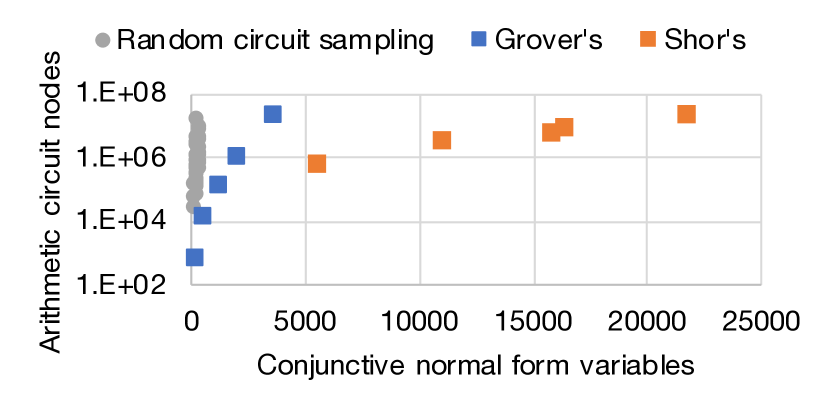
Figure 6. Simulation resource requirements vs. quantum circuit size for three quantum algorithms.

Table 4. Problem size metrics for largest instances in Figure 6.

	# qubits	# gates	AC file size
RCS	42	840	82 MB
Grover’s	17	2460	530 MB
Shor’s	13	12247	586 MB

3.2.3. Evaluation of Knowledge Compilation on Quantum Algorithm Case Studies

As we will demonstrate next for a variety of structured and unstructured quantum circuits, the compiled AC representations avoid the worst case and offer reductions in simulation complexity.

Figure 6 plots the resource requirements of a simulation against the underlying quantum circuit size for various quantum algorithm simulation workloads. The horizontal axis counts the number of variables in the CNF (and in the Bayesian network); this value is proportional to the number of gates inside the quantum algorithm quantum circuit. The vertical axis, in log scale, counts the number of nodes in the compiled AC; this number is proportional to several measures of the simulation resource intensiveness, including the number of edges in the AC, the memory and filesize needed to store the AC, and the time to compile and perform inference on the AC.

The data points in the plot correspond to simulation instances of various sizes (Table 4) belonging to three quantum algorithms. Two of the three algorithms are structured workloads, meaning that they are designed to perform a meaningful computation. The orange data points are instances of Shor’s factoring algorithm (Shor, 1997), written in a style that minimizes qubit count (Beauregard, 2003). The circuits here are factoring either 6 or 15, covering a range of one through four iterations of the algorithm. The blue data points are instances of Grover’s search algorithm (Grover, 1996, 2001). In this case the algorithm is searching for the square root of a number in a simple abstract algebra setting, for a search space ranging from two to 16 elements. The implementations are taken from open source quantum algorithm benchmarks, and the simulation results are validated to be correct outputs.

The third algorithm is an unstructured workload, meaning that the quantum operations are randomly selected and placed in a fixed template. These problems in random circuit sampling (RCS) are extremely difficult to simulate because the qubits rapidly become entangled with all other qubits (Boixo et al., 2018; Harrow and Montanaro, 2017; Terhal, 2018), leaving little independence structure for knowledge compilation to exploit. The gray data points are simulations of a population of such workloads involving between 25 and 42 qubits.

The trends here on a semi-log plot show different scaling trends among the three workloads. The RCS workload exhibits full exponential growth in simulation difficulty, while the Grover’s and Shor’s workloads appear to scale sub-exponentially. This is a result of the knowledge compilation toolchain extracting structure with different degrees of success for the three classes of workloads. The significance of this capability is that we can repurpose knowledge compilation to extract structure and reduce the cost of simulating a quantum circuit.

3.3. Calculating Amplitudes and Sampling from Arithmetic Circuits

The ACs that result from the previous program transformations dictate the minimal sequence of calculations for both finding amplitudes for a given set of qubit states (Section 3.3.1) and also sampling outcomes from the final wavefunction (Section 3.3.2), for a given quantum circuit topology and a given variable order. These two tasks proceed, respectively, as upward and downward traversals of the AC graph. The ACs memoize calculation results from previous queries so that only changed nodes have to be recalculated for new queries.

ACs such as the one in Figure 5 consists of nodes that are either operations (multiply, add) or leaves. The leaves represent either numerical parameters—quantum amplitudes (e.g., $1/\sqrt{2}$) and noise probabilities (e.g., $0.6$)—or logical variables representing qubit states (e.g., ${\color[rgb]{0,0,1}\texttt{q0m1}=\ket{0}}$). The actual values describing quantum amplitudes and noise probabilities can vary between simulation runs as they vary across variational algorithm iterations. Likewise, the truth values for the qubit state assignments can vary to find the amplitude of any output qubit state of interest.

Table 5. Upward pass for finding amplitudes.

q0m2rv	q0m1	q1m3	amplitude	density matrix component
0	$\ket{0}$	$\ket{0}$	$1/\sqrt{2}$	$\begin{bmatrix}+\frac{1}{2}&0&0&+\frac{0.8}{2}\\ 0&0&0&0\\ 0&0&0&0\\ +\frac{0.8}{2}&0&0&+\frac{0.64}{2}\end{bmatrix}$
0	$\ket{0}$	$\ket{1}$	$0$
0	$\ket{1}$	$\ket{0}$	$0$
0	$\ket{1}$	$\ket{1}$	$0.8/\sqrt{2}$
1	$\ket{0}$	$\ket{0}$	$0$	$\begin{bmatrix}0&0&0&0\\ 0&0&0&0\\ 0&0&0&0\\ 0&0&0&+\frac{0.36}{2}\end{bmatrix}$
1	$\ket{0}$	$\ket{1}$	$0$
1	$\ket{1}$	$\ket{0}$	$0$
1	$\ket{1}$	$\ket{1}$	$-0.6/\sqrt{2}$

3.3.1. Calculating Amplitudes via Inference on ACs

Our simulator calculates the amplitude for a given output basis state by finding the probability amplitude of such evidence in the Bayesian network. Such a calculation proceeds as an upward traversal of the AC in Figure 5 following the procedure by Darwiche (Darwiche, 2003, 2009).

Now, let’s see the traversal procedure in action. The white insets in Figure 5 contain a pair of values: the left one tracks the upward traversal for finding the amplitude while the right one tracks the downward traversal for sampling to be discussed next in Section 3.3.2. Suppose we want to find the probability amplitude for the $\ket{11}$ output state, given that the q0m2rv noise event does occur. The simulator assigns the value 1 to the logical variable nodes for $\texttt{q0m2rv}=1$, ${\color[rgb]{0,0,1}\texttt{q0m1}=\ket{1}}$, and ${\color[rgb]{1,.5,0}\texttt{q1m3}=\ket{1}}$, indicating that they are true; and it assigns 0 to the logical variable nodes that indicate otherwise. The calculations dictated by the operator nodes lead to a root node value at the top of $-0.6/\sqrt{2}$, corresponding to the probability amplitude of the assigned output qubit state and noise events.

Following the same procedure above, Table 5 completes the calculation of the probability amplitude for all other sets of noise event (q0m2rv) and qubit states (q0m1, q1m3) assignments, leading to probability amplitudes for eight different possibilities. The two different assignments for the noise event, $\texttt{q0m2rv}=0$ and $\texttt{q0m2rv}=1$, lead to two density matrix components that sum up to the overall density matrix of

$$\rho=\begin{bmatrix}\frac{1}{2}&0&0&\frac{0.8}{2}\\ 0&0&0&0\\ 0&0&0&0\\ \frac{0.8}{2}&0&0&\frac{1}{2}\end{bmatrix}$$

which is exactly the expected final density matrix result in Equation 3 for the noisy Bell-state creation circuit in Figure 2(a) with $\ket{00}$ as the input.

It is worth emphasizing that all of the compilation and simulation techniques we describe up to this point are exact and involve no approximations. Because the compilation and simulation is exact, we can validate that our simulator gives exactly the right probability amplitude distributions across all of the measurement outcomes. We validate the overall simulation approach by creating a new simulator backend for the Google Cirq open-source framework for quantum programming. The simulator passes a suite of randomized validation tests for ideal noise-free state vector simulation and also noisy density matrix simulation. We also demonstrate correct simulation results for a benchmark suite of quantum algorithms, including the CHSH inequality protocol (Clauser et al., 1969), Deutsch-Jozsa (Deutsch and Jozsa, 1992), Bernstein-Vazirani (Bernstein and Vazirani, 1997), Simon’s (Simon, 1997), hidden shift (van Dam et al., 2003), quantum Fourier transform, Shor’s (Shor, 1997), and Grover’s (Grover, 1996) algorithms.

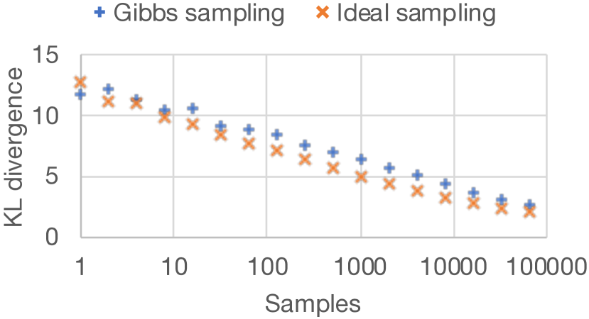
(a) Sampling error for a 16-qubit noise-free QAOA circuit.

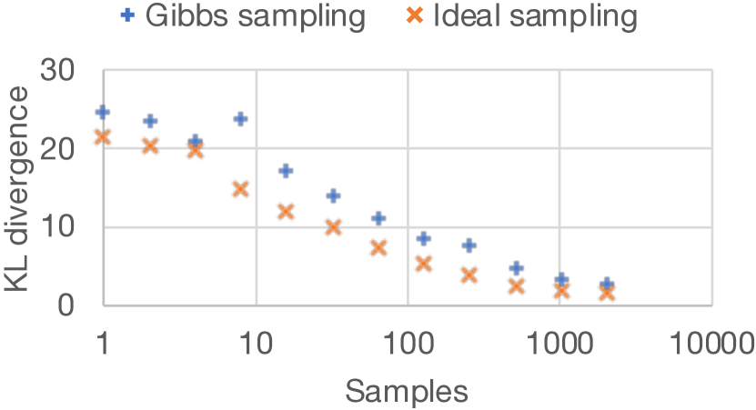
(b) Sampling error for an 8-qubit noisy QAOA circuit.

Figure 7. Sampling error for ideal sampling and Gibbs sampling versus number of samples

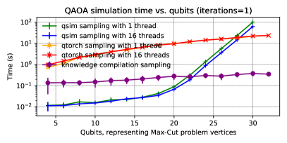
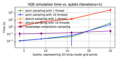
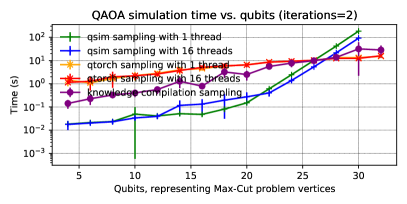
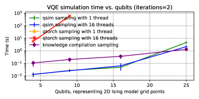
Figure 8. Knowledge compilation vs. state vector (qsim) vs. tensor network (qTorch) performance for ideal (noise-free) circuits

3.3.2. Drawing Samples with Distributions Matching the Output Wavefunction

The final step of our toolchain is to use the compiled arithmetic circuits to approximately sample from the final wavefunction. Such a feature is important in simulating variational quantum algorithms where a few high-probability quantum measurement outcomes most strongly influence the classical optimizer’s objective function (Figure 3). Since a few basis states dominate the output wavefunction, it is easier for the simulator to sample those high probability outcomes than to calculate the full wavefunction. This task of obtaining a sequence of outcomes matching the probability distribution from measuring the final wavefunction amounts to a Markov chain Monte Carlo (MCMC) problem (Chib and Greenberg, 1995).

The compiled AC representation of noisy quantum circuits facilitates Gibbs sampling. Gibbs sampling is a form of MCMC where the next sample of variable assignments is drawn from the variable assignments that are “one away” from the current assignment. More concretely, if the present variable assignment is { $\texttt{q0m2rv}=1$, ${\color[rgb]{0,0,1}\texttt{q0m1}=\ket{1}}$, ${\color[rgb]{1,.5,0}\texttt{q1m3}=\ket{1}}$ }, then the Gibbs sampling MC would consider the following possibilities as the next sample:

• { $\texttt{q0m2rv}=0$, ${\color[rgb]{0,0,1}\texttt{q0m1}=\ket{1}}$, ${\color[rgb]{1,.5,0}\texttt{q1m3}=\ket{1}}$ }

• { $\texttt{q0m2rv}=1$, ${\color[rgb]{0,0,1}\texttt{q0m1}=\ket{0}}$, ${\color[rgb]{1,.5,0}\texttt{q1m3}=\ket{1}}$ }

• { $\texttt{q0m2rv}=1$, ${\color[rgb]{0,0,1}\texttt{q0m1}=\ket{1}}$, ${\color[rgb]{1,.5,0}\texttt{q1m3}=\ket{0}}$ }

Each of these assignments has one of the variable assignments flipped with respect to the present sample.

The compiled arithmetic circuit offers a way to compute the probability of each of the transitions as a downward traversal of the AC (Darwiche, 2009). To find the transition probabilities, we first find the amplitude for a given set of parameters and evidence via an upward traversal in the AC as in Section 3.3.1, filling in the left number in the white insets in Figure 5. Then, in a downward traversal of the AC, we add to the right number of each node the node’s contribution to the final amplitude, following the procedure by Darwiche (Darwiche, 2003). This right number is the transition probability that helps pick the next step in the MCMC chain.

3.3.3. Evaluation of Sampling Accuracy for Noise-Free and Noisy Circuits

Now, we quantify the extent to which the Gibbs MCMC sampling technique facilitated by arithmetic circuits returns the same distribution, compared to ideal (direct) sampling from a fully-known final wavefunction. We are interested in this evaluation because this final sampling step in our simulation toolchain is an approximation technique, in contrast to the prior steps where the noisy quantum circuits are exactly translated into Bayesian networks, CNFs, and arithmetic circuits with no approximation. As shown in Figure 3, the distribution given by Gibbs sampling (Figure 3d) introduces inaccuracy compared to ideal sampling (Figure 3c) from a known wavefunction (Figures 3a and 3b). This inaccuracy is due to warmup and mixing requirements for the Gibbs sampling MCMC.

Figure 7 plots the error of Gibbs sampling and ideal sampling versus the number of samples taken, for simulating both a noise-free and a noisy quantum circuit. We use the Kullback-Leibler divergence (relative entropy) metric (MacKay, 2002, Chapter 2.8) to quantify the difference between the sampled distribution versus the fully known distribution. We choose this metric (in contrast to other metrics such as $\chi^{2}$) because the KL divergence discounts any error due to zero samples being drawn from low-probability outcomes. We sample outcomes from a QAOA Max-Cut benchmark circuit involving 16 qubits in the noise-free and 8 qubits in the noisy case. In the noisy case, the noise model is a symmetric depolarizing noise channel with 0.5% probability of occurence after each gate. The trends show that both sampling approaches converge to the same distribution with increasing number of samples. The Gibbs sampling approach has slightly worse accuracy versus ideal sampling due to the aforementioned MCMC warmup and mixing issues.

This evaluation shows that, for simulating variational algorithms where measurement probabilities are sharply peaked, the Gibbs sampling approach facilitated via knowledge compilation returns a correct distribution with sufficient samples.

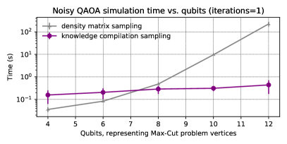
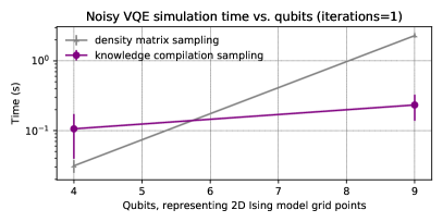
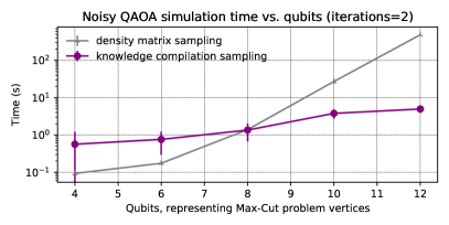
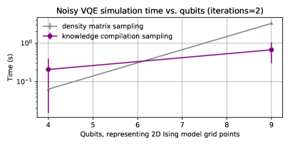
Figure 9. Knowledge compilation vs. density matrix simulation performance for noisy circuits

Table 6. Intermediate compilation result metrics for largest problem instances in Figures 8 and 9.

		# qubits	# gates (# BN nodes)	# CNF clauses	# AC nodes	# AC edges	AC size
	QAOA 1 iteration	32	240	1440	3139	7959	50.7 KB
Ideal	QAOA 2 iterations	32	416	2592	3934271	9635580	84.8 MB
(Figure 8)	VQE 1 iteration	25	169	839	1334	2975	26.2 KB
	VQE 2 iterations	25	309	1579	79056	188328	1.4 MB
	QAOA 1 iteration	12	378	3996	5798	9415	43 KB
Noisy	QAOA 2 iterations	12	516	5292	18991	39839	304.4 KB
(Figure 9)	VQE 1 iteration	9	272	2867	3810	5758	47.9 KB
	VQE 2 iterations	9	343	3637	7701	13941	107.5 KB

4. Evaluation of Sampling Performance for Ideal and Noisy Circuits

With the correctness of our knowledge compilation and simulation approach established, in this section we benchmark our approach on variational algorithm noisy quantum circuits. We compare against three existing major classes of quantum circuit simulators: state vector, density matrix, and tensor network based simulators.

For problem sizes corresponding to near-term quantum applications (beyond eight noisy qubits with ~12 gates per qubit), we demonstrate that the knowledge compilation approach has an advantage over the simulators that tabulate the entire quantum state (i.e., state vector and density matrix simulators), while knowledge compilation’s performance advantage relative to tensor network methods depends on the circuit topology.

4.1. Evaluation for Ideal Circuit Simulation and Sampling

In Figure 8, we compare our simulator against qsim, a state vector simulator by Google that was a component of their quantum supremacy validation experiments (team and collaborators, 2020). qsim is a C-based SIMD simulator that works by multiplying gate unitary matrices against a large state vector. We also compare against qTorch, a tensor-network simulator (Fried et al., 2018). We selected qTorch as a comparison baseline because it is recent, open source, and intended for arbitrary quantum circuits, in contrast to other tensor network simulators that have stipulations on qubit connectivity and the type of simulated quantum circuit.

We evaluate the simulators on two representative variational algorithms, QAOA and VQE. The QAOA workload (Figure 8 and 8) solves a Max-Cut problem on random graphs with varying number of vertices each having three edges. Each qubit encodes one vertex, and two-qubit gates between qubits encode the connectivity of the random graphs (Farhi et al., 2014; Szegedy, 2019). The VQE workload (Figure 8 and 8) finds the minimum energy configuration for a 2D Ising model problem. Each qubit encodes a grid point in 2D space, and two-qubit gates between qubits encode couplings between electron spins (Barahona, 1982). For both problems, we perform one or two iterations of the quantum circuit, where the two iteration version would have higher concentration of higher probability outcomes, at the cost of doubling the circuit depth.

For each problem combination, we plot the time it takes to draw 1000 samples against the number of qubits. The data points are averages across ~16 Nelder-Mead optimization runs with randomized problem instances.

At 30 qubits, the qsim state vector simulator has to hold in memory a vector of $2^{30}\approx 1.1\mathrm{B}$ complex numbers, which accounts for state vector simulation’s exponential cost per simulation run relative to the number of qubits. The knowledge compilation and tensor network simulators use circuit representations that avoid such a storage cost. Table 6 summarizes metrics for the knowledge compilation intermediate results for the largest problem instances.

The ability for knowledge compilation and tensor network simulators to handle circuit depth (in the form of algorithm iterations) depends on the quantum circuit topology: At one algorithm iteration, knowledge compilation needs $66\times$ less time than the tensor network method per sample for 32-qubit QAOA; at two algorithm iterations, the two approaches are comparable for QAOA while qTorch struggles for VQE (Fried et al., 2018).

The results show that for wide (more than 20 noise-free qubits) and shallow (~12 gates per qubit) circuits, the knowledge compilation approach excels at drawing samples from the output wavefunction. These time savings accumulate over the course of a full simulation for a variational quantum algorithm, as the classical optimizer would draw from these distributions many times in order to evaluate the objective function for different input parameters.

4.2. Evaluation for Noisy Circuit Simulation and Sampling

In Figure 9, we compare our simulator against the density matrix simulator for noisy circuits in Google Cirq. The density matrix simulator is a NumPy-based simulator that works by multiplying gate unitary matrices against a large density matrix for mixed quantum states.

We evaluate on QAOA and VQE as before, this time adding a symmetric depolarizing noise channel with 0.5% probability that one of Pauli-X, Y, or Z noise events may happen after each gate. We further validate that the knowledge compilation simulator calculates the same density matrix as the baseline Google Cirq simulator.

At 12 qubits, the Google Cirq density matrix simulator has to hold in memory a matrix of $2^{12}\times 2^{12}\approx 17M$ complex numbers; furthermore the matrix has little sparsity to reduce its representation. Table 6 again summarizes metrics for the knowledge compilation intermediate results.

For noisy circuits, the knowledge compilation approach breaks even with the density matrix simulator at eight qubits, fewer than the case for ideal circuits. This is due to the even greater cost of having to perform matrix-matrix multiplication in density matrix simulation, and also due to less prior focus in developing high performance simulators such as qsim and qTorch for noisy circuit simulation. The data suggest that knowledge compilation is well-suited for the repeated simulation of noisy circuits in variational quantum algorithms.

Table 7. Comparison of quantum and probabilistic graphical models of computation.

	Probabilistic	Quantum
Key analogies	inference	program simulation
	random variables	qubits
	probabilities	amplitudes
	conditional probability tables	operator unitary matrices
	joint probability distributions	superposition states
	dependent random variables	entangled qubits
	variable elimination	tensor network contraction
	weighted model counting (Kimmig et al., 2017)	Feynman path sum
Key distinctions	probabilities between 0 and 1	amplitudes are complex-valued
	probabilities sum to 1	squares of absolute amplitudes sum to 1
	interference impossible	interference (canceling of amplitudes) possible
	equivalent to Clifford set (Van Den Nes, 2010)	beyond Clifford gate set

5. Research Directions

Compiling noisy quantum circuits to PGMs and logical abstractions such as CNFs and arithmetic circuits may accelerate the pace of quantum computing research by offering new ways to analyze quantum circuits. Table 7 lays out loosely analogous concepts between probabilistic and quantum graphical models. The fact that Bayesian networks can be generalized to work on complex-valued quantum amplitudes (Tucci, 1995), along with the insight that knowledge compilation works on algebraic semirings such as complex numbers (Kimmig et al., 2017), underpins the validity of our quantum circuit compilation and simulation toolchain.

This work has focused on finding amplitudes for qubit state assignments and sampling from wavefunctions, by performing a procedure analogous to finding evidence probabilities and gradients via weighted model counting in classical PGMs. The fact that our quantum circuit simulator gives correct results suggests that other types of PGM query techniques (Holtzen et al., 2019, 2020) can likewise support quantum computing research.

Bayesian networks support various other queries such as sensitivity analysis (Darwiche, 2009, Chapter 16)(Laskey, 1995) and most probable explanation (MPE) queries. Sensitivity analysis queries would answer how internal qubit states influence observed qubit states, which may have applications in mapping the most influential qubits variables in an algorithm to the most reliable hardware qubits in a prototype quantum computer. MPE queries would answer what error event best explains a given symptomatic observed outcome. MPE queries rely on the existence of a meaningful operator for finding the maximum value of two quantities; while such a MAX operator is undefined for complex-valued amplitudes, it does exist for real-valued error probabilities. These other types of queries can be made tractable, depending on the algebraic properties of what the Bayesian networks represent, and depending on the choice of the knowledge compilation target representation (Kimmig et al., 2011, 2017; Choi et al., 2020).

6. Conclusion

This paper proposes and evaluates a new quantum circuit simulation technique that focuses on simulating NISQ era variational quantum algorithms. Our simulation toolchain extends techniques originating in classical exact probabilistic inference to support this important quantum simulation workload. Our simulator compiles noisy quantum circuits into complex-valued Bayesian networks in order to combine real-valued noise probabilities and complex-valued quantum amplitudes in one graphical notation. Our simulator then uses knowledge compilation, a technique originally meant for repeated inference, to form an arithmetic circuit that encodes structure information about the quantum circuit. The pre-compiled information then allows for efficient repeated quantum circuit simulation with different parameters, and allows for efficient Gibbs sampling from the output wavefunction. We validated the simulation approach for a benchmark suite of quantum algorithms. For wide and shallow quantum circuits found in variational algorithms such as QAOA and VQE, our simulator performance compares favorably against both ideal and noisy quantum circuit simulators. These simulation capabilities may accelerate the development of useful quantum computing systems and near-term quantum algorithms.

Appendix A Artifact Appendix

A.1. Abstract

This artifact demonstrates a new way to perform quantum circuit simulation. We convert quantum circuits into probabilistic graphical models, which are then compiled into a format that enables efficient repeated queries.

The artifact consists of a Docker image which includes Google Cirq, a quantum programming framework, which we have extended to use our proposed approach as a quantum circuit simulation backend. Also in the Docker image are two quantum circuit simulators based on existing approaches which we compare against as evaluation baselines.

We offer the Docker image via three routes: a hosted version on Docker Hub provides the latest version of our software and requires minimal setup; a Dockerfile is provided to show how to replicate our environment from scratch; and finally a stable archival version is available on Zenodo.

With minimal setup, you can run test cases in our Docker container showing the validity of our approach. We test our quantum circuit simulation approach using the randomized test harness that Google Cirq uses to test its quantum circuit simulation back ends. We also demonstrate correct simulation results for a benchmark suite of quantum algorithms.

The Docker image contains performance benchmarking experiments that replicate results of our paper at reduced input problem sizes. The experiment scripts generate PDFs showing graphs that plot simulation wall clock time against input quantum circuit sizes. The input problem sizes are large enough to show that our proposed approach achieves a speedup versus existing simulation tools.

A.2. Artifact Check-List (Meta-Information)

• Algorithm: A new algorithm for simulating quantum circuits and quantum noise models.

• Program: Google Cirq https://github.com/quantumlib/Cirq, UCLA Ace compiler http://reasoning.cs.ucla.edu/ace/, Google qsim https://github.com/quantumlib/qsim, qTorch https://github.com/aspuru-guzik-group/qtorch.

• Transformations: The quantum circuits and noise models are converted to complex-valued Bayesian networks. A set of techniques originating in Bayesian inference, known as knowledge compilation, converts the Bayesian networks into logical formulas that support repeated queries.

• Model: A benchmark suite of quantum circuits provided in Google Cirq.

• Run-time environment: The Docker container has been tested on Linux (Ubuntu 18.04.5 LTS) and macOS (Big Sur Version 11.1).

• Hardware: 8 GB memory is needed to run the reduced-size validation test suites. Additional memory (up to 1 TB) is recommended to replicate the paper results for the largest problem instances.

• Execution: Less than 30 minutes to run the reduced size validation test suites.

• Metrics: Quantum circuit simulation times for our proposed simulator compared against three baseline simulators from prior work.

• Output: Four PDF files plotting wall clock times for sampling outputs plotted against quantum circuit size.

• Experiments: Pull Docker image (or load from tarball), run Docker container, and call various Python scripts within container.

• How much disk space required (approximately)?: 4 GB

• How much time is needed to prepare workflow?: 10 minutes

• How much time is needed to complete experiments (approximately)?: 30 minutes

• Publicly available?: https://hub.docker.com/repository/docker/yipenghuang0302/quantum_knowledge_compilation

• Archived (provide DOI)?:

  https://doi.org/10.5281/zenodo.4321945
  

A.3. Description

A.3.1. How to Access

Our experiment requires setting up Docker (https://docs.docker.com/get-started/). The Docker container requires about 4 GB of free disk space. We provide three ways to access our experiment environment:

1. Pulling the latest Docker image from Docker Hub (recommended);

2. Downloading Docker image tarball from Zenodo (for artifact archiving purposes);

3. Building a new image from a Dockerfile which pulls from GitHub repositories (demonstrates how to replicate the experiment environment).

Below, we provide instructions for accessing our artifact via each approach.

Pulling from Docker Hub

From the Unix command line:

⬇

$ docker pull yipenghuang0302/\

quantum_knowledge_compilation:latest

Downloading from Zenodo archive

1. Obtain the Docker image tarball from Zenodo at this DOI:

   https://doi.org/10.5281/zenodo.4321945
   

2. Then, load the Docker image tarball:

   ⬇

   $ docker load --input \

   quantum_knowledge_compilation.tar.gz

Building from Dockerfile

1. Download the Ace compiler from http://reasoning.cs.ucla.edu/ace/download.php.

2. Obtain the Dockerfile on GitHub:

   ⬇

   $ git clone \

   https://github.com/ \

   yipenghuang0302/Cirq.git

3. Place the Ace compiler tarball in the same directory as the Dockerfile:

   ⬇

   $ mv ace_v3.0_linux86.tar.gz \

   Cirq/kc_examples

4. Change your working directory to the same directory as the Dockerfile, and build the Docker image:

   ⬇

   $ cd Cirq/kc_examples

   $ docker build \

   --tag quantum_knowledge_compilation .

A.3.2. Hardware Dependencies

• We tested our experiment artifact on a Linux desktop and on an Apple MacBook Pro laptop (2019, with 16 GB of RAM).

• The full experimental results involving the largest problem instances in our paper were done on a Linux server (Two Intel Skylake Xeon Gold 6148 CPUs @ 2.40 GHz and 1 TB of RAM).

A.3.3. Software Dependencies

As you can see from the Dockerfile, the experiment relies on various pieces of software outlined in our checklist:

• Google Cirq, a quantum programming framework: https://github.com/quantumlib/Cirq

• bayes-to-cnf, a Bayesian network compiler that outputs conjunctive normal form logical formulas: https://github.com/gisodal/bayes-to-cnf

• UCLA Ace compiler, a knowledge compilation tool that supports efficient repeated inference: http://reasoning.cs.ucla.edu/ace/

• Google qsim, a quantum circuit simulator based on matrix vector multiplication, which we compare against as a baseline: https://github.com/quantumlib/qsim

• qTorch, a quantum circuit simulator based on tensor network contraction, which we compare against as a baseline: https://github.com/aspuru-guzik-group/qtorch

These software dependencies are automatically downloaded and compiled in the Docker image.

A.3.4. Data Sets

We use a benchmark suite of quantum circuits in Google Cirq to validate our simulator and to measure its performance. These input data sets are included in the Google Cirq repository, and are automatically downloaded in the Docker image.

A.4. Installation

No special installation is needed after you have obtained the Docker image via one of the sources above. Just enter the Docker container:

⬇

$ docker run -ti \

-v $(pwd):/common/home/yh804/research/pdfs \

yipenghuang0302/\

quantum_knowledge_compilation:latest

• The -ti flag makes the Docker container interactive.

• The -v flag binds the directory
  /common/home/yh804/research/pdfs/ inside the Docker container to the present working directory of the host machine. We will be moving the experiment output plots to the host machine through this volume binding.

A.5. Experiment Workflow

We will perform two types of experiments in this artifact demonstration. First, we will run a set of tests that validate the correctness of our proposed quantum circuit simulator. Second, we will evaluate the performance of our simulation approach against three baseline quantum circuit simulators from prior work.

A.5.1. Validation

From the directory that you first arrive in the Docker container (/common/home/yh804/research/), run the following Python test suites, which should take less than 5 minutes:

⬇

$ pytest Google/Cirq/ \

cirq/sim/kc_sparse_simulator_test.py

$ pytest Google/Cirq/ \

kc_examples/kc_examples_test.py

A.5.2. Performance Evaluation

From the directory that you first arrive in the Docker container (/common/home/yh804/research/), run the following performance benchmarking experiments, which should take less than 20 minutes combined.

⬇

$ python3 Google/Cirq/kc_examples/\

kc_qtorch_qaoa/kc_qtorch_qaoa.py

$ python3 Google/Cirq/kc_examples/\

kc_qtorch_vqe/kc_qtorch_vqe.py

$ python3 Google/Cirq/kc_examples/\

kc_noise_qaoa/kc_noise_qaoa.py

$ python3 Google/Cirq/kc_examples/\

kc_noise_vqe/kc_noise_vqe.py

After running the performance benchmarks, move the experimental result PDF files to the host machine through the volume binding:

⬇

$ mv *.pdf /common/home/yh804/research/pdfs/

A.6. Evaluation and Expected Result

Here we describe the validation test suites and their expected results. We then describe the expected trends in the performance benchmarking results.

A.6.1. Validation

We ran two Python test suites during the validation step, and both should return no errors. They test the following:

kc_sparse_simulator_test

We show that our simulation approach passes test cases that the Google Cirq framework uses to validate simulator back ends.

kc_examples_test

We show that our simulation approach gives correct results for a benchmark suite of quantum algorithms implemented in Google Cirq, including:

1. Bernstein-Vazirani algorithm

2. Bell state creation

3. Bell inequality

4. Deutsch’s algorithm

5. Grover’s algorithm

6. Hidden shift algorithm

7. Simon’s algorithm

8. Quantum Fourier transform

9. Quantum teleportation

A.6.2. Performance Evaluation

The performance plot PDF files replicate the results presented in Figures 8 (sampling from noise-free quantum circuits) and 9 (sampling from noisy quantum circuits) of the paper submission, albeit at reduced input sizes to reduce time and hardware requirements. The problem sizes are large enough to show that our simulation approach has an advantage vs. the baseline simulators. An example result is included here in Figure 10.

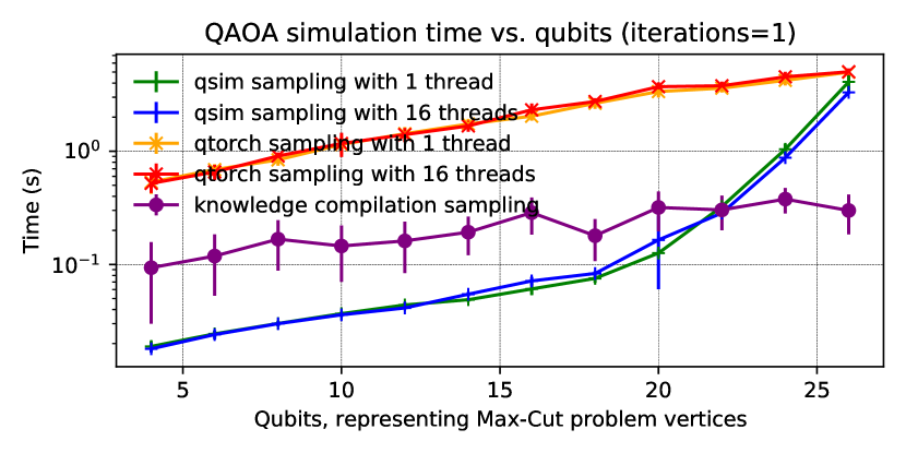
Figure 10. Example output of kc_qtorch_qaoa.py: time to sample outputs from noise-free circuits for the QAOA quantum algorithm.

A.7. Experiment Customization

The experiment input size parameters can be adjusted in the Python files kc_qtorch_qaoa.py, kc_qtorch_vqe.py, kc_noise_qaoa.py, and kc_noise_vqe.py:

• The max_length parameter controls the quantum circuit width, the number of qubits in the input circuit.

• The p or the step parameter controls the quantum circuit depth, the number iterations of the input circuit.

A.8. Methodology

Submission, reviewing and badging methodology:

• www.acm.org/publications/policies/artifact-review-badging

• cTuning.org/ae/submission-20201122.html

• cTuning.org/ae/reviewing-20201122.html

References

- (1)
- Allen et al. (2017) John-Mark A. Allen, Jonathan Barrett, Dominic C. Horsman, Ciarán M. Lee, and Robert W. Spekkens. 2017. Quantum Common Causes and Quantum Causal Models. Physical Review X 7, 3, Article 031021 (Jul 2017), 031021 pages. https://doi.org/10.1103/PhysRevX.7.031021 arXiv:1609.09487 [quant-ph]
- Anschuetz et al. (2019) Eric Anschuetz, Jonathan Olson, Alán Aspuru-Guzik, and Yudong Cao. 2019. Variational Quantum Factoring. In Quantum Technology and Optimization Problems, Sebastian Feld and Claudia Linnhoff-Popien (Eds.). Springer International Publishing, Cham, 74–85.
- Arute et al. (2019) Frank Arute, Kunal Arya, Ryan Babbush, Dave Bacon, Joseph C. Bardin, Rami Barends, Rupak Biswas, Sergio Boixo, Fernando G. S. L. Brandao, David A. Buell, Brian Burkett, Yu Chen, Zijun Chen, Ben Chiaro, Roberto Collins, William Courtney, Andrew Dunsworth, Edward Farhi, Brooks Foxen, Austin Fowler, Craig Gidney, Marissa Giustina, Rob Graff, Keith Guerin, Steve Habegger, Matthew P. Harrigan, Michael J. Hartmann, Alan Ho, Markus Hoffmann, Trent Huang, Travis S. Humble, Sergei V. Isakov, Evan Jeffrey, Zhang Jiang, Dvir Kafri, Kostyantyn Kechedzhi, Julian Kelly, Paul V. Klimov, Sergey Knysh, Alexander Korotkov, Fedor Kostritsa, David Landhuis, Mike Lindmark, Erik Lucero, Dmitry Lyakh, Salvatore Mandrà, Jarrod R. McClean, Matthew McEwen, Anthony Megrant, Xiao Mi, Kristel Michielsen, Masoud Mohseni, Josh Mutus, Ofer Naaman, Matthew Neeley, Charles Neill, Murphy Yuezhen Niu, Eric Ostby, Andre Petukhov, John C. Platt, Chris Quintana, Eleanor G. Rieffel, Pedram Roushan, Nicholas C. Rubin, Daniel Sank, Kevin J. Satzinger, Vadim Smelyanskiy, Kevin J. Sung, Matthew D. Trevithick, Amit Vainsencher, Benjamin Villalonga, Theodore White, Z. Jamie Yao, Ping Yeh, Adam Zalcman, Hartmut Neven, and John M. Martinis. 2019. Quantum supremacy using a programmable superconducting processor. Nature 574, 7779 (2019), 505–510. https://doi.org/10.1038/s41586-019-1666-5
- Arute et al. (2020) Frank Arute, Kunal Arya, Ryan Babbush, Dave Bacon, Joseph C. Bardin, Rami Barends, Sergio Boixo, Michael Broughton, Bob B. Buckley, David A. Buell, Brian Burkett, Nicholas Bushnell, Yu Chen, Zijun Chen, Ben Chiaro, Roberto Collins, William Courtney, Sean Demura, Andrew Dunsworth, Edward Farhi, Austin Fowler, Brooks Foxen, Craig Gidney, Marissa Giustina, Rob Graff, Steve Habegger, Matthew P. Harrigan, Alan Ho, Sabrina Hong, Trent Huang, L. B. Ioffe, Sergei V. Isakov, Evan Jeffrey, Zhang Jiang, Cody Jones, Dvir Kafri, Kostyantyn Kechedzhi, Julian Kelly, Seon Kim, Paul V. Klimov, Alexander N. Korotkov, Fedor Kostritsa, David Landhuis, Pavel Laptev, Mike Lindmark, Martin Leib, Erik Lucero, Orion Martin, John M. Martinis, Jarrod R. McClean, Matt McEwen, Anthony Megrant, Xiao Mi, Masoud Mohseni, Wojciech Mruczkiewicz, Josh Mutus, Ofer Naaman, Matthew Neeley, Charles Neill, Florian Neukart, Hartmut Neven, Murphy Yuezhen Niu, Thomas E. O’Brien, Bryan O’Gorman, Eric Ostby, Andre Petukhov, Harald Putterman, Chris Quintana, Pedram Roushan, Nicholas C. Rubin, Daniel Sank, Kevin J. Satzinger, Andrea Skolik, Vadim Smelyanskiy, Doug Strain, Michael Streif, Kevin J. Sung, Marco Szalay, Amit Vainsencher, Theodore White, Z. Jamie Yao, Ping Yeh, Adam Zalcman, and Leo Zhou. 2020. Quantum Approximate Optimization of Non-Planar Graph Problems on a Planar Superconducting Processor. arXiv:2004.04197 [quant-ph]
- Barahona (1982) F Barahona. 1982. On the computational complexity of Ising spin glass models. Journal of Physics A: Mathematical and General 15, 10 (oct 1982), 3241–3253. https://doi.org/10.1088/0305-4470/15/10/028
- Beauregard (2003) Stephane Beauregard. 2003. Circuit for Shor’s Algorithm Using 2N+3 Qubits. Quantum Info. Comput. 3, 2 (March 2003), 175–185. http://dl.acm.org/citation.cfm?id=2011517.2011525
- Bernstein and Vazirani (1997) Ethan Bernstein and Umesh Vazirani. 1997. Quantum Complexity Theory. SIAM J. Comput. 26, 5 (1997), 1411–1473. https://doi.org/10.1137/S0097539796300921 arXiv:https://doi.org/10.1137/S0097539796300921
- Biamonte and Bergholm (2017) Jacob Biamonte and Ville Bergholm. 2017. Tensor Networks in a Nutshell. arXiv e-prints, Article arXiv:1708.00006 (Jul 2017), arXiv:1708.00006 pages. arXiv:1708.00006 [quant-ph]
- Boixo et al. (2018) Sergio Boixo, Sergei V. Isakov, Vadim N. Smelyanskiy, Ryan Babbush, Nan Ding, Zhang Jiang, Michael J. Bremner, John M. Martinis, and Hartmut Neven. 2018. Characterizing quantum supremacy in near-term devices. Nature Physics 14, 6 (2018), 595–600. https://doi.org/10.1038/s41567-018-0124-x
- Boixo et al. (2017) Sergio Boixo, Sergei V Isakov, Vadim N Smelyanskiy, and Hartmut Neven. 2017. Simulation of low-depth quantum circuits as complex undirected graphical models. arXiv preprint arXiv:1712.05384 (2017).
- Bravo-Prieto et al. (2019) Carlos Bravo-Prieto, Ryan LaRose, M. Cerezo, Yigit Subasi, Lukasz Cincio, and Patrick J. Coles. 2019. Variational Quantum Linear Solver: A Hybrid Algorithm for Linear Systems. arXiv:1909.05820 [quant-ph]
- Chavira et al. (2005) Mark Chavira, David Allen, and Adnan Darwiche. 2005. Exploiting Evidence in Probabilistic Inference. In Proceedings of the Twenty-First Conference on Uncertainty in Artificial Intelligence (Edinburgh, Scotland) (UAI’05). AUAI Press, Arlington, Virginia, United States, 112–119. http://dl.acm.org/citation.cfm?id=3020336.3020350
- Chavira and Darwiche (2005) Mark Chavira and Adnan Darwiche. 2005. Compiling Bayesian Networks with Local Structure. In Proceedings of the 19th International Joint Conference on Artificial Intelligence (Edinburgh, Scotland) (IJCAI’05). Morgan Kaufmann Publishers Inc., San Francisco, CA, USA, 1306–1312. http://dl.acm.org/citation.cfm?id=1642293.1642501
- Chavira and Darwiche (2006) Mark Chavira and Adnan Darwiche. 2006. Encoding CNFs to Empower Component Analysis. In Theory and Applications of Satisfiability Testing - SAT 2006, Armin Biere and Carla P. Gomes (Eds.). Springer Berlin Heidelberg, Berlin, Heidelberg, 61–74.
- Chavira and Darwiche (2008) Mark Chavira and Adnan Darwiche. 2008. On Probabilistic Inference by Weighted Model Counting. Artif. Intell. 172, 6-7 (April 2008), 772–799. https://doi.org/10.1016/j.artint.2007.11.002
- Chib and Greenberg (1995) Siddhartha Chib and Edward Greenberg. 1995. Understanding the Metropolis-Hastings algorithm. The american statistician 49, 4 (1995), 327–335.
- Choi et al. (2020) YooJung Choi, Antonio Vergari, and Guy Van den Broeck. 2020. Probabilistic Circuits: A Unifying Framework for Tractable Probabilistic Models. (2020).
- Clauser et al. (1969) John F. Clauser, Michael A. Horne, Abner Shimony, and Richard A. Holt. 1969. Proposed Experiment to Test Local Hidden-Variable Theories. Phys. Rev. Lett. 23 (Oct 1969), 880–884. Issue 15. https://doi.org/10.1103/PhysRevLett.23.880
- Cross et al. (2019) Andrew W. Cross, Lev S. Bishop, Sarah Sheldon, Paul D. Nation, and Jay M. Gambetta. 2019. Validating quantum computers using randomized model circuits. Phys. Rev. A 100 (Sep 2019), 032328. Issue 3. https://doi.org/10.1103/PhysRevA.100.032328
- Darwiche (2002) Adnan Darwiche. 2002. A Logical Approach to Factoring Belief Networks. In Proceedings of the Eights International Conference on Principles of Knowledge Representation and Reasoning (Toulouse, France) (KR’02). Morgan Kaufmann Publishers Inc., San Francisco, CA, USA, 409–420. http://dl.acm.org/citation.cfm?id=3087093.3087128
- Darwiche (2003) Adnan Darwiche. 2003. A Differential Approach to Inference in Bayesian Networks. J. ACM 50, 3 (May 2003), 280–305. https://doi.org/10.1145/765568.765570
- Darwiche (2009) Adnan Darwiche. 2009. Modeling and Reasoning with Bayesian Networks (1st ed.). Cambridge University Press, New York, NY, USA.
- Darwiche and Marquis (2002) Adnan Darwiche and Pierre Marquis. 2002. A knowledge compilation map. Journal of Artificial Intelligence Research 17 (2002), 229–264.
- Deutsch (1989) D. Deutsch. 1989. Quantum Computational Networks. Proceedings of the Royal Society of London. Series A, Mathematical and Physical Sciences 425, 1868 (1989), 73–90. http://www.jstor.org/stable/2398494
- Deutsch and Jozsa (1992) David Deutsch and Richard Jozsa. 1992. Rapid Solution of Problems by Quantum Computation. Proceedings of the Royal Society of London Series A 439, 1907 (Dec. 1992), 553–558. https://doi.org/10.1098/rspa.1992.0167
- Farhi et al. (2014) Edward Farhi, Jeffrey Goldstone, and Sam Gutmann. 2014. A Quantum Approximate Optimization Algorithm. arXiv e-prints, Article arXiv:1411.4028 (Nov 2014), arXiv:1411.4028 pages. arXiv:1411.4028 [quant-ph]
- Farhi and Harrow (2016) Edward Farhi and Aram W Harrow. 2016. Quantum Supremacy through the Quantum Approximate Optimization Algorithm. arXiv:1602.07674 [quant-ph]
- Feynman (2006) Richard Phillips Feynman. 2006. QED: The strange theory of light and matter. Princeton University Press.
- Fried et al. (2018) E. Schuyler Fried, Nicolas P. D. Sawaya, Yudong Cao, Ian D. Kivlichan, Jhonathan Romero, Alán Aspuru-Guzik, and Itay Hen, ed. 2018. qTorch: The quantum tensor contraction handler. PLoS ONE 13, 12 (12 2018). https://doi.org/10.1371/journal.pone.0208510
- Grover (1996) Lov K. Grover. 1996. A Fast Quantum Mechanical Algorithm for Database Search. In Proceedings of the Twenty-eighth Annual ACM Symposium on Theory of Computing (Philadelphia, Pennsylvania, USA) (STOC ’96). ACM, New York, NY, USA, 212–219. https://doi.org/10.1145/237814.237866
- Grover (2001) Lov K. Grover. 2001. From Schrödinger’s equation to the quantum search algorithm. American Journal of Physics 69, 7 (2001), 769–777. https://doi.org/10.1119/1.1359518 arXiv:https://doi.org/10.1119/1.1359518
- Harrow and Montanaro (2017) Aram W. Harrow and Ashley Montanaro. 2017. Quantum computational supremacy. Nature 549 (13 09 2017), 203 EP –. https://doi.org/10.1038/nature23458
- Henson et al. (2014) Joe Henson, Raymond Lal, and Matthew F Pusey. 2014. Theory-independent limits on correlations from generalized Bayesian networks. New Journal of Physics 16, 11 (nov 2014), 113043. https://doi.org/10.1088/1367-2630/16/11/113043
- Holtzen et al. (2019) Steven Holtzen, Todd Millstein, and Guy Van den Broeck. 2019. Generating and Sampling Orbits for Lifted Probabilistic Inference. In Proceedings of the 35th Conference on Uncertainty in Artificial Intelligence (UAI).
- Holtzen et al. (2020) Steven Holtzen, Guy Van den Broeck, and Todd Millstein. 2020. Scaling Exact Inference for Discrete Probabilistic Programs. Proc. ACM Program. Lang. (OOPSLA) (2020). https://doi.org/10.1145/342820
- Huang et al. (2019) Hsin-Yuan Huang, Kishor Bharti, and Patrick Rebentrost. 2019. Near-term quantum algorithms for linear systems of equations. arXiv:1909.07344 [quant-ph]
- Huang and Martonosi (2019a) Yipeng Huang and Margaret Martonosi. 2019a. QDB: From Quantum Algorithms Towards Correct Quantum Programs. In 9th Workshop on Evaluation and Usability of Programming Languages and Tools (PLATEAU 2018) (OpenAccess Series in Informatics (OASIcs), Vol. 67), Titus Barik, Joshua Sunshine, and Sarah Chasins (Eds.). Schloss Dagstuhl–Leibniz-Zentrum fuer Informatik, Dagstuhl, Germany, 4:1–4:14. https://doi.org/10.4230/OASIcs.PLATEAU.2018.4
- Huang and Martonosi (2019b) Yipeng Huang and Margaret Martonosi. 2019b. Statistical Assertions for Validating Patterns and Finding Bugs in Quantum Programs. In Proceedings of the 46th International Symposium on Computer Architecture (Phoenix, AZ) (ISCA ’19).
- Kaye et al. (2007) Phillip Kaye, Raymond Laflamme, and Michele Mosca. 2007. An Introduction to Quantum Computing. Oxford University Press, Inc., New York, NY, USA.
- Kimmig et al. (2011) Angelika Kimmig, Guy Van den Broeck, and Luc De Raedt. 2011. An Algebraic Prolog for Reasoning about Possible Worlds. In Proceedings of the Twenty-Fifth AAAI Conference on Artificial Intelligence (San Francisco, California) (AAAI’11). AAAI Press, 209–214.
- Kimmig et al. (2017) Angelika Kimmig, Guy Van den Broeck, and Luc De Raedt. 2017. Algebraic Model Counting. J. of Applied Logic 22, C (July 2017), 46–62. https://doi.org/10.1016/j.jal.2016.11.031
- Koller and Friedman (2009) Daphne Koller and Nir Friedman. 2009. Probabilistic Graphical Models: Principles and Techniques - Adaptive Computation and Machine Learning. The MIT Press.
- Korb and Nicholson (2010) Kevin B. Korb and Ann E. Nicholson. 2010. Bayesian Artificial Intelligence, Second Edition (2nd ed.). CRC Press, Inc., Boca Raton, FL, USA.
- Laskey (1995) K. B. Laskey. 1995. Sensitivity analysis for probability assessments in Bayesian networks. IEEE Transactions on Systems, Man, and Cybernetics 25, 6 (1995), 901–909.
- Lubasch et al. (2020) Michael Lubasch, Jaewoo Joo, Pierre Moinier, Martin Kiffner, and Dieter Jaksch. 2020. Variational quantum algorithms for nonlinear problems. Phys. Rev. A 101 (Jan 2020), 010301. Issue 1. https://doi.org/10.1103/PhysRevA.101.010301
- MacKay (2002) David J. C. MacKay. 2002. Information Theory, Inference & Learning Algorithms. Cambridge University Press, USA.
- Markov and Shi (2008) I. Markov and Y. Shi. 2008. Simulating Quantum Computation by Contracting Tensor Networks. SIAM J. Comput. 38, 3 (2008), 963–981. https://doi.org/10.1137/050644756 arXiv:https://doi.org/10.1137/050644756
- Markov et al. (2018) Igor L Markov, Aneeqa Fatima, Sergei V Isakov, and Sergio Boixo. 2018. Quantum supremacy is both closer and farther than it appears. arXiv preprint arXiv:1807.10749 (2018).
- Mermin (2007) N.D. Mermin. 2007. Quantum Computer Science: An Introduction. Cambridge University Press.
- National Academies of Sciences, Engineering, and Medicine (2019) National Academies of Sciences, Engineering, and Medicine. 2019. Quantum Computing: Progress and Prospects. The National Academies Press, Washington, DC. https://doi.org/10.17226/25196
- Nielsen and Chuang (2011) Michael A. Nielsen and Isaac L. Chuang. 2011. Quantum Computation and Quantum Information: 10th Anniversary Edition (10th ed.). Cambridge University Press, New York, NY, USA.
- Pearl (2014) Judea Pearl. 2014. Probabilistic reasoning in intelligent systems: networks of plausible inference. Elsevier.
- Peruzzo et al. (2014) Alberto Peruzzo, Jarrod McClean, Peter Shadbolt, Man-Hong Yung, Xiao-Qi Zhou, Peter J. Love, Alán Aspuru-Guzik, and Jeremy L. O’Brien. 2014. A variational eigenvalue solver on a photonic quantum processor. Nature Communications 5 (23 07 2014), 4213 EP –. http://dx.doi.org/10.1038/ncomms5213
- Pienaar and Brukner (2015) Jacques Pienaar and Časlav Brukner. 2015. A graph-separation theorem for quantum causal models. New Journal of Physics 17, 7, Article 073020 (Jul 2015), 073020 pages. https://doi.org/10.1088/1367-2630/17/7/073020 arXiv:1406.0430 [quant-ph]
- Preskill (2018) John Preskill. 2018. Quantum Computing in the NISQ era and beyond. Quantum 2 (Aug. 2018), 79. https://doi.org/10.22331/q-2018-08-06-79
- Resch and Karpuzcu (2019) Salonik Resch and Ulya R. Karpuzcu. 2019. Benchmarking Quantum Computers and the Impact of Quantum Noise. arXiv:1912.00546 [quant-ph]
- Sang et al. (2005) Tian Sang, Paul Bearne, and Henry Kautz. 2005. Performing Bayesian Inference by Weighted Model Counting. In Proceedings of the 20th National Conference on Artificial Intelligence - Volume 1 (Pittsburgh, Pennsylvania) (AAAI’05). AAAI Press, 475–481. http://dl.acm.org/citation.cfm?id=1619332.1619409
- Shor (1997) P. Shor. 1997. Polynomial-Time Algorithms for Prime Factorization and Discrete Logarithms on a Quantum Computer. SIAM J. Comput. 26, 5 (1997), 1484–1509. https://doi.org/10.1137/S0097539795293172 arXiv:https://doi.org/10.1137/S0097539795293172
- Simon (1997) Daniel R. Simon. 1997. On the Power of Quantum Computation. SIAM J. Comput. 26, 5 (1997), 1474–1483. https://doi.org/10.1137/S0097539796298637 arXiv:https://doi.org/10.1137/S0097539796298637
- Szegedy (2019) Mario Szegedy. 2019. What do QAOA energies reveal about graphs? arXiv:1912.12277 [quant-ph]
- team and collaborators (2020) Quantum AI team and collaborators. 2020. qsim. https://doi.org/10.5281/zenodo.4023103
- Terhal (2018) Barbara M. Terhal. 2018. Quantum supremacy, here we come. Nature Physics 14, 6 (2018), 530–531. https://doi.org/10.1038/s41567-018-0131-y
- Tucci (1995) Robert R Tucci. 1995. Quantum Bayesian nets. Int. Journal of Modern Physics B 9, 03 (1995), 295–337.
- van Dam et al. (2003) Wim van Dam, Sean Hallgren, and Lawrence Ip. 2003. Quantum Algorithms for Some Hidden Shift Problems. In Proceedings of the Fourteenth Annual ACM-SIAM Symposium on Discrete Algorithms (Baltimore, Maryland) (SODA ’03). Society for Industrial and Applied Mathematics, USA, 489–498.
- Van Den Nes (2010) Maarten Van Den Nes. 2010. Classical Simulation of Quantum Computation, the Gottesman-Knill Theorem, and Slightly Beyond. Quantum Info. Comput. 10, 3 (March 2010), 258–271. http://dl.acm.org/citation.cfm?id=2011350.2011356
- Yeang (2010) C. Yeang. 2010. A Probabilistic Graphical Model of Quantum Systems. In 2010 Ninth International Conference on Machine Learning and Applications. 155–162. https://doi.org/10.1109/ICMLA.2010.30