Mechanical properties of DNA and DNA nanostructures: comparison of atomistic, Martini and oxDNA

Abstract

The flexibility and stiffness of small DNA play a fundamental role ranging from several biophysical processes to nano-technological applications. Here, we estimate the mechanical properties of short double-stranded DNA (dsDNA) having length ranging from 12 base-pairs (bps) to 56 bps, paranemic crossover (PX) DNA, and hexagonal DNA nanotubes (DNTs) using two widely used coarse-grain models – Martini and oxDNA. To calculate the persistence length ($L_{p}$) and the stretch modulus ($\gamma$) of the dsDNA, we incorporate the worm-like chain and elastic rod model, while for DNT, we implement our previously developed theoretical framework. We compare and contrast all the results with previously reported all-atom molecular dynamics (MD) simulation and experimental results. The mechanical properties of dsDNA ($L_{p}$ $\sim$ 50nm, $\gamma$ $\sim$ 800-1500 pN), PX DNA ($\gamma$ $\sim$ 1600-2000 pN) and DNTs ($L_{p}$ $\sim$ 1-10 $\mu$m, $\gamma$ $\sim$ 6000-8000 pN) estimated using Martini soft elastic network and oxDNA are in very good agreement with the all-atom MD and experimental values, while the stiff elastic network Martini reproduces order of magnitude higher values of $L_{p}$ and $\gamma$. The high flexibility of small dsDNA is also depicted in our calculations. However, Martini models proved inadequate to capture the salt concentration effects on the mechanical properties with increasing salt molarity. oxDNA captures the salt concentration effect on small dsDNA mechanics. But it is found to be ineffective to reproduce the salt-dependent mechanical properties of DNTs. Also, unlike Martini, the time evolved PX DNA and DNT structures from the oxDNA models are comparable to the all-atom MD simulated structures. Our findings provide a route to study the mechanical properties of DNA and DNA based nanostructures with increased time and length scales and has a remarkable implication in the context of DNA nanotechnology.

I Introduction

DNA, the genetic information carrier of life, having contour length of few cm to meters, has to undergone twisting, bending, stretching to be packaged into a cell of few $\mu$m diameterPurohit et al. (2003). To facilitate such packaging into the cell, DNA is wrapped around oppositely charged histone proteins in a highly organized structure known as nucleosome core particle (NCP)Richmond and Davey (2003). Several other fundamental biological processes such as transcriptions, replications, gene expression are also bringing in mechanical stress to DNABustamante et al. (1994); Maier et al. (2000); Parvin et al. (1995); Perez-Martin and Espinosa (1993). In most of these biological processes, the length scales of DNA involved are of few tens of base pairs and much smaller than its persistence length ($\sim$50 nm)Baumann et al. (1997); Shore et al. (1981); Smith et al. (1992). Hence, understanding the mechanics of small DNA is of key interest in the field of molecular biology.

Sequence specificity of DNA has made it possible to utilize it as an ideal building block to create a wide variety of complex nanostructuresSeeman (2003). Utilizing the key properties of DNA such as its persistence length and Watson-Crick sequence specificity, nanometer-scale devices and material can be created. The idea of the DNA nanotechnology field was first led by N. C. Seeman in 1982 who designed a four-armed junction, a cube, a truncated octahedron in several stagesChen and Seeman (1991); Fu and Seeman (1993); Kallenbach et al. (1983); Seeman (2003); Zhang and Seeman (1994). Seeman’s visionary idea is now rapidly developing the field of DNA nanotechnology because of its potential application in drug delivery, synthetic biology and DNA computingBhatia et al. (2016); Langecker et al. (2012); Lee et al. (2012); Maiti et al. (2004, 2006); Pinheiro et al. (2011); Seeman (2003, 2007); Walsh et al. (2011). In another approach namely ‘DNA origami’, recently established by P. Rothemund, a long DNA strand can be folded using small DNA staple strands and can be very efficient in designing complex DNA nanostructuresRothemund (2006). DNA nanotube (DNT), a programable biomimicking ion-channel, is one of the recent additions of the expanding repository of DNA nanostructuresJoshi et al. (2015); Kuzuya et al. (2007); Lin et al. (2007); Rothemund et al. (2004); Wang et al. (2012). Once properly derivatized, DNT can spontaneously insert into the lipid membrane and have appeared to function as an ion channel and can also transport drug molecules across the cell membranesBurns et al. (2014, 2013a, 2013b); Gopfrich et al. (2016); Harrell et al. (2004); Joshi et al. (2016); Joshi and Maiti (2017); Naskar et al. (2019a); Yoo and Aksimentiev (2013). Also, DNT can be operated as a robotic arm to carry and transport cargo across the cell and can also perform as a support system for other cell membrane channelsKopperger et al. (2018). Enhanced Rigidity of DNTs have widespread applications from nanoelectronics to nanomechanical devicesKuzuya et al. (2007); Liu et al. (2004); Lo et al. (2010); Wang et al. (2012); Yoo and Aksimentiev (2015). Thus, the mechanical strength of the DNTs is one of the most essential aspects and considerable effort has been put to measure and increase the mechanical strength of these nanotubes.

During the last few decades, with the advancement of single-molecule manipulation techniques, our understanding of DNA and DNA nanostructure’s mechanics has expanded immenselyAggarwal et al. (2020); Baumann et al. (1997); Bustamante et al. (2003, 1994); Gross et al. (2011a); Smith et al. (1996, 1992); Wiggins et al. (2006). Utilizing experimental techniques such as optical trapping, magnetic tweezers, atomic force microscopy (AFM), it has now turn out to be feasible to externally pull DNA at different physiological conditionsBustamante et al. (2003); Marko and Siggia (1995); Santosh and Maiti (2009); Smith et al. (1996, 1992). Although the mechanics of DNA is highly dependent on the sequence and physiological condition, most of these pulling experiments are suitably described by a worm-like chain (WLC) modelBustamante et al. (2003). AFM studies by Mazur et al. observed that the WLC model can properly capture the flexibility of short DNA beyond two helical turnsMazur and Maaloum (2014a, b). However, some experimental studies challenged the validity of the WLC model for very short DNA and at high force regimes. Modifications have been made to the WLC model (such as twistable worm-like chain model, linear sub elastic chain model) to explain the mechanics of DNA at high force regimesGross et al. (2011b); Noy and Golestanian (2012); Ranjith et al. (2005). Likewise, to obtain the mechanical properties of DNTs, the contour length and end-to-end distances have been extracted from fluorescence images and then fitted to the WLC model to estimate their values of persistence lengthWang et al. (2012). In a recent study by Liu et. al, combining small-angle Xray scattering (SAXS) and Förster resonance energy transfer (FRET) characterization with MD simulation, estimated structural and mechanical properties of DNA in a variety of physiological conditionsLiu et al. (2018a).

Computational modeling like molecular dynamics or density functional theory can play a key role given the fact that sometimes experiments are very difficult to perform routinely. Also, it is challenging to obtain high-resolution structural information from experiments. Theoretical models and all-atom simulations can be very effective in predicting structural and mechanical properties prior to the experimental realizationsChakraborty et al. (2009); Maiti et al. (2004, 2006); Naskar et al. (2020); Nomidis et al. (2017); Skoruppa et al. (2018); Zoli (2018, 2019); Orozco et al. (2003, 2008). Notably, Maiti and coworkers implemented the WLC and elastic rod model to study the mechanics of dsDNA and DNA based nanostructures like paranemic crossover (PX/JX) DNA molecules, DNA nanotubes, and found their elastic properties to be in close agreement with the experimental resultsGarai et al. (2015); Joshi et al. (2015, 2016); Joshi and Maiti (2017); Mogurampelly et al. (2013); Naskar et al. (2019a); Sahoo et al. (2019).

Simulating fully atomistic models of dsDNA and DNA nanostructures are computationally very demanding. A less computationally expensive and highly efficient approach is the coarse-grained modeling in which the basic units are no longer single atom, but some larger units – be it some atoms, or a nucleotide, a base pair or a double helixArbona et al. (2012); Mergell et al. (2003); Ouldridge et al. (2011); Snodin et al. (2015); Šulc et al. (2012); Uusitalo et al. (2015, 2017). Coarse-grained simulations averages over the nonessential degrees of freedom and thus reduces the complexity of the fully atomistic simulations. Therefore, such methods inevitably lose structural details of the systems and accuracy of the physical properties depend on the level of parameterization but can be very effective in studying system over longer time and length scales. In this study, we have used two widely used coarse-grained DNA models – Martini and oxDNA to understand the mechanics of short DNAs and DNA based nanostructures. The organization of the paper is as follows: In the method section, we give a brief description of the models followed by the simulation methodology. We then provide the theory used in this study to estimate the mechanical properties of DNAs and DNTs. In the result section, we present our calculation of stretch modulus and persistence lengths of dsDNA having various lengths, PX DNA and DNT and compare those with all-atom simulation results. Finally, we conclude and provide appealing future directions.

II Methods

II.1 Martini model

The coarse-grained (CG) Martini model of DNA is parameterized by combining top-down information derived from the experiment and bottom-up knowledge gained from the atomistic simulations. For each residue, the beads are divided into side-chain beads (SC1, SC2, SC3, SC4) and backbone beads (BB1, BB2, BB3). The backbone of the DNA is modeled with three beads – one for phosphate group (BB1 bead) and the other two represents the sugar moiety (BB2 and BB3). Roughly four non-hydrogen atoms are mapped to one CG bead. The pyrimidines (C and T) are mapped as three beads and the purines (A and G) are mapped as four beads. SC1 and SC2 beads form base-pair when they are in opposite strands. The CG representation of Martini model is illustrated in figure 1a. The backbone beads are modeled with a large sphere with diameter $\sigma$= 0.47 nm (for sugar beads $\sigma$= 0.43 nm). Since the bases are stacked very closely to each other with a distance of 0.34 nm, these CG beads with such high $\sigma$ will lead to overlapping with each other. For this reason and also to maintain the planarity of the bases, a small CG bead with $\sigma$= 0.32 nm is parameterized to characterize the bases. The interaction potential, $V$ is composed of bonded interaction, $V_{bonded}$ and non-bonded interactions, $V_{non-bonded}$. The bonded potential is composed of usual harmonic bond, angle and dihedral potential. The bonded interactions are modeled in a manner that reproduces bond, angle and dihedral distributions obtained from the atomistic MD simulations. The non-bonded potential is composed of Columbic interaction between charge particles and Van der Waals interaction. The bead types are selected by comparing the calculated partitioning free energies of DNAs in water, chloroform and hydrated octanol with available experimental data. To incorporate the hydrogen bond interactions between the nucleobases, the interaction is tuned between the hydrogen-bonded beads. An elastic network has been implemented in order to maintain the canonical form of the dsDNA. All the beads are chargeless expect the one representing the phosphate group, which has been assigned with -1e charge. Like all CG models, Martini also has its advantages and disadvantages. The partitioning free-energy of nucleobases in the Martini model is comparable to the experimental values. In some cases, it reproduces better results than the all-atom force-fields. The radius of gyration of ssDNA and ion distribution around DNA are also reproduced reasonably well compared to those obtained at the all-atom level. The two different types of elastic networks serve different purposes and the choice of the network will depend on the particular need in the application. The current limitation of the model is the reduced strength of the base-pairing interactions. Also, the hydrogen bonds between the base pairs do not have depends on the angle, which prevents this model from studying DNA hybridization, melting, hairpin formation, or intercalation. For a detailed description of the Martini model, the reader is recommended to go through the original references Marrink et al. (2007); Uusitalo et al. (2015, 2017).

II.2 OxDNA model

The CG oxDNA model is parameterized with a top-down approach, aimed to include the thermodynamic transition of DNAOuldridge et al. (2011); Snodin et al. (2015); Šulc et al. (2012). Each strand of dsDNA is constructed using a chain of CG beads. Each nucleobase is represented by a single CG bead as illustrated in figure 1b. For the phosphate backbone, another CG bead is assigned (See Figure 1b). There are three interaction sites for each nucleotide and they lie in a straight line. The three interaction sites are the hydrogen-bonding site, base stacking site and backbone excluded volume site. A normal vector is defined to specify the orientational plane of the bases. Each CG bead is interacting with others in a pairwise fashion with excluded volume, stacking, hydrogen-bonding (HB), cross-stacking interaction and co-axial stacking (c-stack). Nearest neighbors (nn) interactions are distinct compared to all other interactions in the strand which permits for stacking and strand connectivity. The potential energy function of the oxDNA model can be written as a sum of the following interactions,

$$V=\sum_{nn}(V_{backbone}+V_{stack}+V_{exc}^{{}^{\prime}})+\sum_{otherpairs}(V_{HB}+V_{cross-stacking}+V_{exc}+V_{c-stack})$$ (1)

The nearest neighbor pairs are interacting via $V_{backbone}$, $V_{stack}$ and $V_{exc}^{{}^{\prime}}$ potentials and the other pairs are interacting with $V_{HB}$, $V_{cross-stacking}$, $V_{exc}$ and $V_{c-stack}$ potentials. $V_{backbone}$ represents the covalent bond between the rigid bodies in the form of a finitely extensible nonlinear elastic (FENE) spring with an equilibrium distance of 6.4 $\AA$ to hold the nucleotides in a strand together. $V_{stack}$ is a smoothly cut-off Morse potential with a minimum at 3.4 $\AA$ to mimic the stacking of the bases in a coplanar manner. $V_{exc}^{{}^{\prime}}$ and $V_{exc}$ are the excluded volume interactions between nearest neighbor and next-nearest neighbor, respectively. It provide the stiffness to unstacked bases of the single strands and prevents crossing of the chains. $V_{HB}$ is a smoothly cut-off Morse potential between hydrogen-bonding sites and provides the hydrogen-bonded interaction for base-pairing. $V_{cross-stacking}$ and $V_{c-stack}$ corresponding to the cross-stacking and co-axial stacking between the non-nearest neighbors, respectively and provides additional stabilization of the duplex. In the oxDNA2 model, which is a revised version of the original oxDNA model, sequence-dependent stacking and hydrogen-bonding interactions are used Šulc et al. (2012). No explicit electrostatic interaction is taken into account in the model. Too include electrostatic effect, Debye-Hückel potential is added in the non-bonded interaction. OxDNA has several advantages over the other CG models. This is the first CG model which captures the three key thermodynamic processes that affect self-assembly– hybridization of double-stranded DNA, single-stranded stacking, hairpin formation. The mechanical properties like stretch modulus, torsional modulus and persistence length are also reasonably well represented by the oxDNA model. The only limitation of this model that it under predict the effect of terminal mismatches, dangling ends, bulges and internal mismatches on the duplex melting temperature. For a detailed description of the oxDNA model, the reader is recommended to the original the references Ouldridge et al. (2011); Snodin et al. (2015); Šulc et al. (2012).

Figure 1: Description of the coarse-grained models and various systems studied in this work. (a) Coarse-grain mapping of Martini DNA. Each base of the DNA is modeled with either three beads (Cytosine and Thymine) or four beads (Adenine and Guanine). The sugar moiety is modeled with two beads and the phosphate group is modeled with a single bead. (b) Coarse-grained oxDNA model. Each nucleotide is modeled with two beads – one for the base (cyan ellipsoid) and another for the backbone (red and blue sphere) of the DNA. Initial structures of dsDNA (c) 12bps (d) 24 bps (e) 38 bps (f) 56 bps. (g) Initial structure of paranemic crossover DNA. (h) Initial model of hexagonal DNA nanotube.

II.3 Simulation procedure

Here, we have studied four dsDNA systems of finite length, 12, 24, 38, and 56 bps, PX DNA, and a hexagonal DNA nanotube originally synthesized by Wang et. al (See figure 1c-h). The sequence of dsDNA, PX DNA and the DNT is provided in the supporting information (SI). The all-atom structures of the dsDNA and the DNT are built using a custom written code in nucleic acid builder (NAB) language of Ambertools. Then the structures are converted to the CG Martini model using Martinize.py codeUusitalo et al. (2015). For each system, two different elastic networks – soft and stiff has been implemented. The structures are then solvated in CG Martini water model and an appropriate number of sodium ion (Na⁺) is added to make the whole system charge neutral. For Martini simulations, we have used two different types of water models in our study –one is standard chargeless Martini CG water model and other one is Martini polarizable water model. We present all the main results for standard Martini CG water model. We have separately discussed the effect of Martini polarizable water model on DNA mechanics later.

The MD simulations of the CG Martini models were performed using Gromacs 5.1 simulation packageVan Der Spoel et al. (2005). All the systems were subjected to the steepest descent energy minimization while keeping restraint on DNA/DNT with a force constant of 20 kJ.mol^-1Å^-2 which was gradually reduced to zero. The systems were then heated to 300 K and equilibrated in the NPT ensemble for 100 ns. The systems were then subjected to 2 $\mu$s long simulation in the NVT ensemble. The time step was taken to be 10 fs for all the simulations. Long-range electrostatic interactions were included using reaction-field with a cutoff of 1.5 nmBarker and Watts (1973). Same cutoff was also used for the short-range part of the Coulomb interaction with the potential shift cutoff scheme. For polarizable water model we have used particle mesh Ewald (PME) method for Coulomb interaction with a cutoff of 1.5 nm. The pair-list was updated after every 10th steps. Temperature regulation was achieved by velocity rescaling thermostat with a time constant of 0.5 psVan Der Spoel et al. (2005). To maintain the pressure at 1.0 bar, Berendsen barostat was used with a time constant of 3.0 ps and a compressibility of $3.0\times 10^{-5}$ bar^-1Berendsen et al. (1984).

For oxDNA models, the structures are directly built using the source codeOuldridge et al. (2011); Snodin et al. (2015); Šulc et al. (2012). MD simulations with the oxDNA model were performed using the source code provided by with oxDNA force fieldOuldridge et al. (2011); Snodin et al. (2015); Šulc et al. (2012). We have simulated the systems for $2\times 10^{8}$ to $2\times 10^{9}$ MD cycle with a time step of 0.005 which in real unit corresponds to a total of 3 $\mu$s to 30 $\mu$s long MD run. Simulations were performed in the NVT ensemble at T = 300 K. Temperature regulation was implemented using Anderson thermostatAndersen (1980).

Analysis of the mechanical properties was done for the last half of the production run. We divided the trajectory equally into 5 segments and for each segment we independently calculated all the relevant properties and finally averaged it over the 5 segments to report the final quantities. Visualization of the systems and trajectories were done using VMDHumphrey et al. (1996) and UCSF ChimeraPettersen et al. (2004). For trajectory analysis purpose we have used CPPTRAJRoe and Cheatham III (2013), MDTRAJMcGibbon et al. (2015), home written python codes and TCL scripts.

II.4 Theory of dsDNA, PX DNA, and DNT mechanics

We estimated the dsDNA stretch modulus by combining microscopic elastic rod theory with the WLC model. We assumed dsDNA as a uniform elastic rod of instantaneous contour length, $L$ at time $t$, which is fluctuating about its equilibrium length $L_{0}$ due to the thermal energy. The definition of dsDNA contour length is given in figure 2. Any fluctuation of length will give rise to a restoring force (F) which is proportional to ($L-L_{0}$) and can be expressed as, $F(L)=-\gamma\ (L-L_{0})/L_{0}$, where $\gamma$ is the stretch modulus of the rod. The energy associated with this force can be obtained by integrating the force with respect to $L$ which gives $E(L)=-\gamma\ (L-L_{0})^{2}/(2L_{0})$. The probability $(P(L))$ of having a rod of length, $L$ with an energy $E(L)$ is then obtained through Boltzmann statisticsGarai et al. (2015); Joshi et al. (2016); Mogurampelly et al. (2013); Naskar et al. (2019a),

$$P(L)=\sqrt{\frac{\gamma\beta}{2\pi\ L_{0}\ }}\ \ exp\left[-\frac{\gamma\beta\ L_{0}}{2}\ \left(\frac{L}{L_{0}}\ -1\right)^{2}\ \right]$$ (2)

Where $\beta=\frac{1}{K_{B}T}\$. From the slope of the straight line of $\ln{P\left(L\right)}$ vs $\left(\frac{L}{L_{0}}-1\right)^{2}$, the stretch modulus has been extracted.

Figure 2: Definition of the contour length and bending angle used in our studies. The spheres represent the center of mass of each base pair. The contour length is calculated by adding the center of mass between two consecutive base pairs as $L=\ \sum_{i=1}^{N}h_{i}$, where $N$ is the number of base-pairs of the dsDNA. The bending angle is defined as angle between the local vectors $\hat{t}(s)$ and $\hat{t}(s^{{}^{\prime}})$ defining the local axial direction of dsDNA such as, $\theta=\cos^{-1}{(\hat{t}\left(s\right).\hat{t}(s^{\prime}))}$.

In order to calculate the bending persistence length $L_{P}$ of dsDNA, we first estimate the distribution of the bending angle ($\theta$). The $\theta$ is defined as the angle between the local vectors $\hat{t}(s)$ and $\hat{t}(s^{\prime})$ defining the local axial direction of dsDNA or DNT such as $\theta=\cos^{-1}{(\hat{t}\left(s\right).\hat{t}(s^{\prime}))}$ , where $s$ parameterize the path of the polymer as $s\in(0,L_{0})$ (see figure 2). Similar to the length fluctuation, the probability distribution of $\theta$ can be expressed as a Gaussian distribution asGarai et al. (2015); Joshi et al. (2016); Mogurampelly et al. (2013); Naskar et al. (2019a),

$$P\left(\theta\right)=\sqrt{\frac{\beta\kappa}{{2\pi L}_{0}}}exp\left[-\frac{\beta\kappa}{{2L}_{0}}\theta^{2}\right]$$ (3)

$$\Rightarrow\ln{P\left(\theta\right)=}-\frac{L_{P}}{L_{0}}\left(1-\cos{\theta}\right)+\frac{1}{2}\ln{\frac{\beta\kappa}{2\pi L_{0}}}$$ (4)

Where $L_{P}=\beta\kappa$ and $\kappa$ is the bending modulus.

One can also estimate the persistence length from the WLC model. In the WLC model the mean square end-to-end distance can be expressed asGarai et al. (2015); Mogurampelly et al. (2013),

$$\langle\ R^{2}\ \rangle=\langle\ \vec{R}.\vec{R}\ \rangle=\langle\ \int_{0}^{L_{0}}\hat{t}\left(s\right)ds\int_{0}^{L_{0}}\hat{t}(s^{\prime})ds^{\prime}\ \rangle$$ (5)

$$\Rightarrow\langle\ R^{2}\ \rangle=\int_{0}^{L_{0}}ds\int_{0}^{L_{0}}\langle\ \hat{t}\left(s\right)\ .\ \hat{t}(s^{\prime})\ \rangle ds^{\prime}\$$ (6)

$$\Rightarrow\langle\ R^{2}\ \rangle=\int_{0}^{L_{0}}ds\int_{0}^{L_{0}}exp\left[-\frac{|s-s^{\prime}|}{L_{P}}\right]\ ds^{\prime}\$$ (7)

$$\Rightarrow\langle\ R^{2}\ \rangle=2L_{P}L_{0}\left[1-\frac{L_{P}}{L_{0}}\left\{1-exp\left(-\frac{L_{0}}{L_{P}}\right)\right\}\right]$$ (8)

Equation 8 can be solved numerically to get the persistence length , $L_{P}$. We referred the persistence length calculated using equation 8 as $L_{P}^{WLC}$.

Furthermore, according to the microscopic elastic theory, for any uniform rod of cross-sectional area A and stretch modulus $\gamma$, Young’s modulus $\left(Y\right)$ is expressed as, $Y\ =\frac{\gamma}{A}$ and the bending modulus is given by, $\kappa=IY$ , where $I$ is the area moment of inertia of the rod. Combining the above relation, we can write the stretch modulus asGarai et al. (2015); Joshi et al. (2016); Naskar et al. (2019a),

$$\gamma=\frac{A\kappa}{I}=\frac{AL_{P}}{\beta I}$$ (9)

We assume the dsDNA as a uniform rod which gives the area moment of inertia, $I=\frac{\pi R_{1}^{4}}{4}$, $R_{1}$ being the radius of the dsDNA. For DNT we explicitly calculate the I asJoshi et al. (2016); Naskar et al. (2019a),

$$I=\frac{1}{2}\left[\sum_{6}{I_{0}+\left(4R_{1}^{2}+2R_{2}^{2}\right)A_{1}+I_{0}\left(16\frac{R_{2}^{2}}{R_{1}^{2}}-10\right)}\right]$$ (10)

$R_{2}$ is the average radius of the DNT. The detail calculation of the $I$ of DNT is given in reference Joshi et al. (2016).

III Results and Discussions

III.1 Mechanical properties of dsDNA

Figure 3: Stretch modulus and persistence length of CG dsDNA having different lengths. The quantities are calculated using equation 2 and 6.

To measure the mechanical properties as mentioned above, we first calculate the contour length distribution and the bending angle distribution of the dsDNA. The contour length is calculated by adding the center of mass of each base pair as shown in figure 2. In order to calculate the bending angle, two local vectors are defined by joining the center of mass of two consecutive base pairs (See figure 2). The end base pairs are not considered as they might fray during the simulation. The angle between the two vectors is defined as the bending angle. In figure S5 of SI we have plotted the contour length and bending angle distribution of a 12 bps dsDNA. By fitting the contour length and bending angle distribution using equation 2 and 4 respectively, we have extracted the stretch modulus ($\gamma$) and persistence length ($L_{p}$) (see figure 3 and table 1). We find that the persistence lengths of the oxDNA model are in close agreement with the values obtained from all atom simulations and match well with experimental valuesBrunet et al. (2015); Garai et al. (2015); Guilbaud et al. (2019); Marin-Gonzalez et al. (2019, 2017); Trizac and Shen (2016); Yuan et al. (2008). The persistence lengths estimated from Martini model with soft elastic network are in the range of 60 to 130 nm and slightly higher than the values obtained using all-atom model and experimental values of $L_{P}$ ($\sim$ 50nm). Additional softening of the elastic network can improve the results but that may lead to numerically unstable simulations. The stretch modulus obtained from soft-Martini and oxDNA models are in very good agreement with the all-atom and literature valuesGarai et al. (2015); Marin-Gonzalez et al. (2017). Furthermore, the CG Martini with stiff elastic network model gives the persistence length and stretch modulus which is an order of magnitude higher (see table S3 of SI). In stiff-Martini, since the force constant of the elastic network is very high, the structures remain highly static and do not exhibit much fluctuation (see figure S3 of SI).

Figure 4: Stretch modulus and persistence length of CG dsDNA having different lengths. The values are obtained from the WLC model (equation 8 and 9).

We have also calculated the persistence length and the stretch modulus form the WLC model (equation 8) and elastic rod theory (equation 9) respectively. In order to calculate the persistence length using equation 8, we first calculate the end-to-end distance of the dsDNA and then numerically solved equation 8 with the persistence length $L_{p}^{WLC}$ as a fitting parameter. The $L_{p}^{WLC}$ is then used in equation 9 to calculate the stretch modulus ($\gamma^{WLC}$). Both the persistence length ($L_{p}^{WLC}$) and the stretch modulus obtained from the WLC model are in close agreement with the values obtained from the all-atom MD simulations (see figure 4 and table 1).

Also, the results from the WLC model are supporting a series of experiments and theoretical results reporting that small DNAs of few tens of bps have very high flexibility than those of kilo bpsMathew-Fenn et al. (2008); Vafabakhsh and Ha (2012); Wiggins et al. (2006); Yuan et al. (2008); Skoruppa et al. (2020). Wiggins et al. using AFM study and WLC model reported that the bending of short DNAs is larger than that of long DNAsWiggins et al. (2006). In another study, Yuan et al. using FRET and SAXS showed that DNAs with length in the range of 15-89 bps have higher flexibility than kilo bps DNAsYuan et al. (2008). They obtained radius of gyration ($R_{g}$) from the scattering dataYuan et al. (2008) and then $L_{P}$ has been obtained by numerically solving the following equation 11,

$$\langle\ R_{g}^{2}\ \rangle=\frac{LL_{P}}{3}-L_{P}^{2}+\frac{2L_{P}^{3}}{L}-\frac{2L_{P}^{4}}{L^{2}}\left[1-exp\left(-\frac{L}{L_{P}}\right)\right]$$ (11)

The values of $L_{P}$ obtained in our coarse grained simulation are very close to the values obtained in the experimentsYuan et al. (2008). In a recent all-atom MD simulation study, Wu et al. reported similar results for small dsDNAWu et al. (2015). Based on the simulation results, they provided an empirical formula of persistence length ($L_{p}$) as a function of DNA bp length ($N$) which follows,

$$L_{P}\left(N\right)=L_{P}^{0}-\frac{A}{\left(B+N\right)}$$ (12)

Figure 5: Length scale-dependent dsDNA flexibility. The persistence length of the all-atom and CG dsDNA is obtained from the WLC model. The experimental persistence length is obtained from the experimental of the short DNAs by Yuan et al.Yuan et al. (2008). The dashed line represents the persistence length of long dsDNA   50 nm. The solid line is the empirical formula given by equation 12.The all-atom data are adapted from the reference Garai et al. (2015); Wu et al. (2015)

where $L_{P}^{0}$ is the persistence length ($\sim$ 50 nm) of kilo base pair long DNA and $N$ is the number of bps. $A$ and $B$ are the fitting parameters and have values 450 nm and 10 respectively. In figure 5 we have plotted equation 12 as a function of $N$ along with the experimental results by Yuan et al.Yuan et al. (2008), all atom results by Garai et al.Garai et al. (2015) and Wu et al.Wu et al. (2015) and our simulation results. In order to compare better, we have also plotted few more data of oxDNA which has same lengths as done by Wu et al.Wu et al. (2015). We find that the $L_{P}$ calculated from all-atom and soft-Martini models are in close agreement with the experiment as well as with empirical equation 12. However, oxDNA as shown in blue diamond matches reasonably well with empirical formula and experimental for dsDNA lengths up to 30 bps.

To understand how salt concentration might affect the mechanical properties of the CG dsDNA we have carried out simulations at two different salt concentrations – 150 mM and 250 mM. Being a highly charged macromolecule, salt is known to have a strong effect on the structural and mechanical properties of DNABrunet et al. (2015); Garai et al. (2015); Naskar et al. (2019b); Wenner et al. (2002).

Figure 6: Salt dependent mechanical properties of dsDNA. (a) Stretch modulus and (b) persistence length of a 12 bps dsDNA in three different salt concentrations. (c) Stretch modulus and (d) persistence length of a 56 bps dsDNA in three different salt concentrations. Salt dependent stretch modulus and persistence length of other lengths of dsDNA has been provided in the supporting information.

According to the Odijk-Skolnick-Fixman (OSF) model the persistence length decreases with ionic strength (I) as   $I^{-1}$Odijk (1977); Skolnick and Fixman (1977). High salt concentration increases the screening of DNA backbone charges, which leads to more flexible dsDNA. Indeed, Garai et al. also concluded a similar trend in their all-atom simulation resultsGarai et al. (2015). Several other studies also established the above resultsBrunet et al. (2015); Guilbaud et al. (2019). But in our Martini CG simulation results, we do not find any such trend. Both the stretch modulus and the persistence lengths almost remained invariant with increasing salt concentration for all the dsDNA lengths studied in this work (see figure 6 and table S2 of SI). $\gamma$ and $L_{P}$ calculated by various methods as has been outlined above showing similar trends. Our simulation results indicate that the mechanics of coarse-grain Martini dsDNA does not depend on the salt concentration. The original Martini force-field paper by Uusitalo et al. also reported that the $L_{P}$ values changed from 68 $\pm$ 14 nm to 78 $\pm$ 11 nm as the NaCl concentration changed from 100mM to 1000mMUusitalo et al. (2015). Within the error bar there is no change in the value of persistence length in going from 100 mM to 1000 mM. We think the less insensitivity of the CG Martini DNA mechanics with salt is because of the large CG beads and the way charge is distributed within the beads. In Martini model, the -1e charge is distributed in a single bead and most of the Na⁺ ions are tightly bound to it. Because of the large radius of the CG beads the Na⁺ ions are not able to penetrate into the DNA grooves and screen the backbone repulsion effectively. As a result, we see no change in the DNA mechanics with increasing salt concentration. In contrast, as reported in the literature, oXDNA model captures the effect of salt concentration on DNA mechanics very wellSnodin et al. (2015). In the original oxDNA paper, Snodin et al reported that the persistence length changes as the salt concentration varied from 100mM to 1000mMSnodin et al. (2015). We observe that for the oxDNA model the persistence length decreases as the salt concentration is increased (see figure 6 and table S4 of SI). The effect of salt concentration becomes more prominent as the length of the dsDNA increases. Also, the stretch modulus increases as the salt concentration increases which is in agreement with many previous theoretical and experimental studies. Adding more salts screen the electrostatic interaction and help decrease the backbone repulsion leading to less fluctuation in the axial direction of the dsDNA. As a result, we observe an increment in the stretch modulus.

We have also performed few simulations of Martini dsDNA with soft elastic network (of lengths 12 bps, 24 bps, 38 bps) using polarizable water (PW) model. The polarizable CG water is made of three beads instead of one as in the standard Martini CG water modelYesylevskyy et al. (2010). The central bead of the PW interacts by LJ potential whereas other two beads which carry a positive and negative charge interacts via a Coulombic interaction only, and lack any LJ interactions. We found that the dsDNA exhibits almost similar structural deviations in the PW bath. The stretch modulus values for 12 bps, 24 bps, 38 bps dsDNA in PW water are found to be around 981 $\pm$ 238, 900 $\pm$ 130, 818 $\pm$ 176 pN respectively. These values are very similar to the of values of 767 $\pm$ 85, 916 $\pm$ 160, 854 $\pm$ 75 pN in standard Martini CG water for 12 bps, 24 bps, 38 bps dsDNA respectively. Similarly, the persistence lengths are 41 $\pm$ 6, 43 $\pm$ 6, 57 $\pm$ 4 nm for 12 bps, 24 bps, 38 bps dsDNA respectively when simulated in PW water.

Figure 7: Instantaneous snapshots of DNA nanostructures. Final structure of paranemic crossover DNA (PX DNA) and 6-helix DNA nanotube (DNT) after long MD simulation. Final structure of PX DNA simulated using (a) all-atom (b) CG soft-Martini (c) CG stiff-Martini and (d) CG oxDNA model. Final structure of DNT simulated using (e) all-atom (f) CG soft-Martini (g) CG stiff-Martini and (h) CG oxDNA model.

III.2 Mechanical properties of DNA nanostructures

Before evaluating the mechanical properties of DNA nanostructures like PX DNA or DNTs , we need to ensure that the time evolved CG structures of these nanostructures are stable and maintain integrity close to the experimental/all-atom structures. We observe that DNA nanostructures modeled with stiff elastic network in Martini framework is very rigid and has very little fluctuation over $\mu$s long simulations. In contrast, DNA nanostructures modeled with soft elastic network in Martini framework deformed and twisted very much and give rise to unrealistic structure. The time evolved oxDNA DNT reproduces reasonable structure and compare well with the all-atom MD simulated structure (see figure 7).

We have also computed the stretch modulus of PX DNA nanostructures using the elastic rod model. In order to calculate the contour length of the PX DNA, we divided the PX DNA into slices along the long axis, taking one base pair from each of the dsDNA. Then we add the center of mass (COM) distance of consecutive slices to get the contour length. The stretch modulus is then calculated using equation 2. The stretch modulus of PX-DNA is found to be 1548 $\pm$ 112 pN, 883 $\pm$ 312.21 pN, and 1758 $\pm$ 153 pN for all-atom, soft-Martini and oxDNA model respectively. Previously, Santosh et al., by implementing non-equilibrium steered MD found that the stretch modulus of PX DNA is in the range of 1300-2300 pNSantosh and Maiti (2011). The all-atom and oxDNA model reproduces the results well within those range. Due to high structural fluctuation soft-Martini model underestimates the stretch modulus.

Figure 8: Stretch modulus and persistence length of CG DNA nanotube. The quantities are calculated using equation 3 and 10.

To calculate the stretch modulus and persistence length of DNT, we employed the same methodologies described earlier to estimate the mechanical properties of DNA. First, we determine the contour length of the DNT at each time step. The length of each dsDNA of the constituent DNT is calculated by adding the COM distance of consecutive bps and then averaged over the six helices to get the contour length. Similar methodologies have been successfully implemented by Maiti and coworkers in their previous studies on DNTsJoshi et al. (2016); Naskar et al. (2019a). We find that the stretch modulus of DNT modeled with oxDNA is closer to the all-atom and experimental values than the soft-Martini DNT (see figure 8 and table 1). This is attributed to the fact that the soft-Martini DNA has a higher stretch modulus than the all-atom DNA which enhances the rigidity of the DNT. The oxDNA modeled DNT reproduces the stretch modulus value more accurately. The calculated stretch modulus is then used in equation 11 to calculate the persistence lengths of the DNTs. Calculated persistence lengths show similar trend as stretch modulus where soft-Martini model predicts slightly higher value compared to the oxDNA which is closer to the all-atom and experimental valuesJoshi et al. (2015, 2016); Naskar et al. (2019a); Wang et al. (2012). As mentioned earlier, the stiff-Martini model of DNT has hardly any fluctuation and calculated stretch modulus and persistence length values are almost double than the experimental and all-atom values (see table S5).

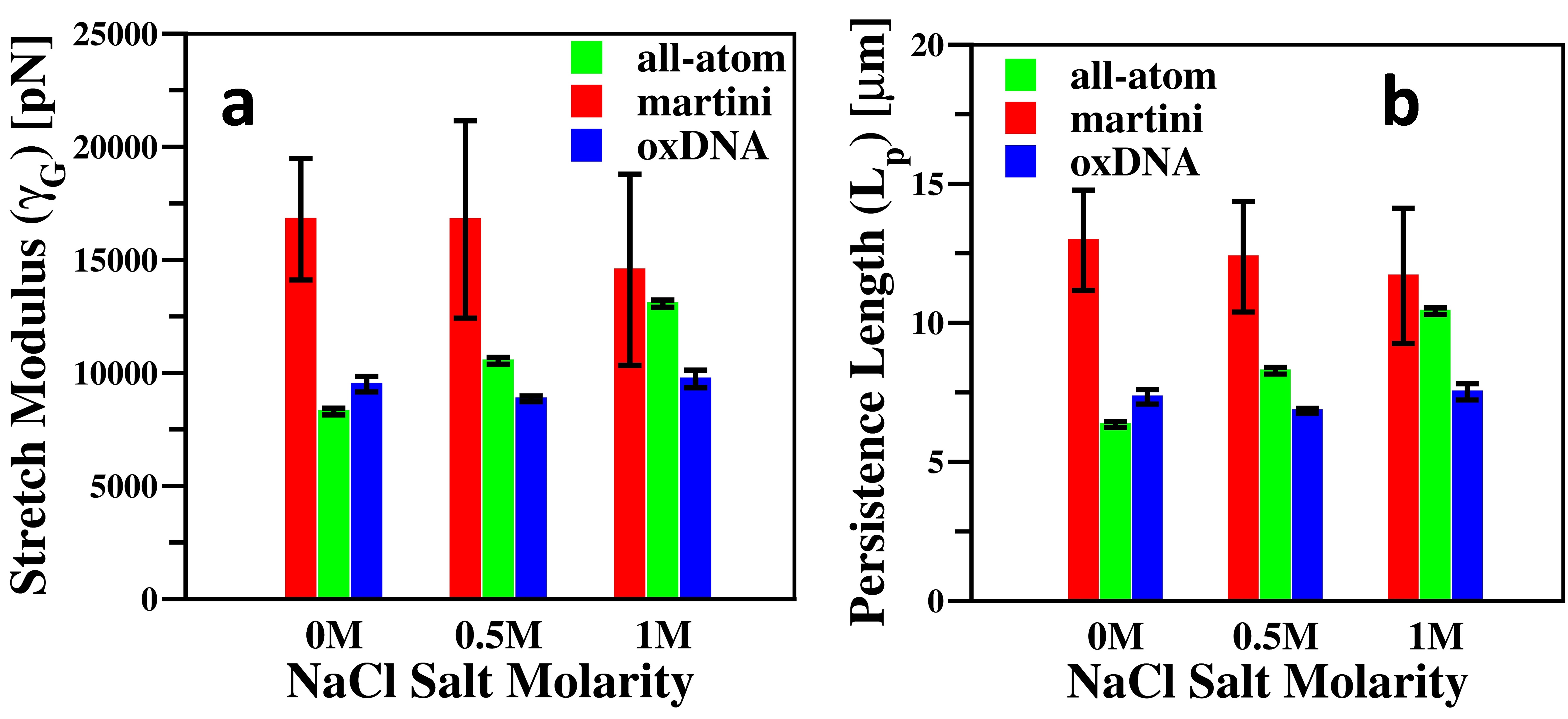
Figure 9: (a) Stretch modulus and (b) persistence lengths of CG DNA nanotubes (DNTs) at different salt concentrations.

Presence of salt is known to have a large impact on the structure and mechanics of DNA nanostructures. Earlier, Naskar et al. have shown that the structural stability and mechanical rigidity of DNT can be increased by increasing monovalent salt concentrationNaskar et al. (2019a). Some recent experimental findings also reported that the charge screening by the MgCl₂ salt reconfigures the structure and mechanics of DNA nanotubesKielar et al. (2018); Liu et al. (2018b). But, in our coarse-grain simulation study, we find the mechanics of DNT remains almost unchanged with salt concentration variation (see figure 9).

Table 1: Mechanical properties of DNA and DNA nanostructures from this study as well as several previous studies.

System	Lengths	Reference	Model	Stretch Modulus (pN)	Persistence Length (nm)
	12 bp			767 ($\gamma_{G}$), 1160 ($\gamma_{WLC}$)	70 ($L_{P}$), 25 ($L^{WLC}_{P}$)
DNA	24 bp	This work	Soft-Martini	916 ($\gamma_{G}$), 1730 ($\gamma_{WLC}$)	104 ($L_{P}$), 29 ($L^{WLC}_{P}$)
	38 bp	(Theory)		855 ($\gamma_{G}$), 1150 ($\gamma_{WLC}$)	69 ($L_{P}$), 30 ($L^{WLC}_{P}$)
	56 bp			1023($\gamma_{G}$), 1946 ($\gamma_{WLC}$)	117 ($L_{P}$), 51 ($L^{WLC}_{P}$)
	12 bp			2152 ($\gamma_{G}$), 728 ($\gamma_{WLC}$)	44 ($L_{P}$), 23 ($L^{WLC}_{P}$)
DNA	24 bp	This work	oxDNA	1470 ($\gamma_{G}$), 825 ($\gamma_{WLC}$)	50 ($L_{P}$), 31 ($L^{WLC}_{P}$)
	38 bp	(Theory)		2210 ($\gamma_{G}$), 1269 ($\gamma_{WLC}$)	77 ($L_{P}$), 52 ($L^{WLC}_{P}$)
	56 bp			1398 ($\gamma_{G}$), 1502 ($\gamma_{WLC}$)	91 ($L_{P}$), 73 ($L^{WLC}_{P}$)
	12 bp			1096 ($\gamma_{G}$), 827 ($\gamma_{WLC}$)	50 ($L_{P}$), 11 ($L^{WLC}_{P}$)
DNA	24 bp	Garai et al.	All-atom	871 ($\gamma_{G}$), 760 ($\gamma_{WLC}$)	46 ($L_{P}$), 44 ($L^{WLC}_{P}$)
	38 bp	(Theory) Garai et al. (2015)		985 ($\gamma_{G}$), 744 ($\gamma_{WLC}$)	45 ($L_{P}$), 50 ($L^{WLC}_{P}$)
	56 bp			1297 ($\gamma_{G}$), 1052 ($\gamma_{WLC}$)	63 ($L_{P}$), 71 ($L^{WLC}_{P}$)
	16 bp	Yuan et al.			20
DNA	21 bp	(experiment)			38
	66 bp	Yuan et al. (2008)			48
			All-atom	1548
PX DNA			Soft-Martini	883
			oxDNA	1758
		Naskar et al. Naskar et al. (2019a)	All-atom	8295	6350
DNA Nanotube (DNT)		This work	Soft-Martini	16800	13520
		This work	oxDNA	9505	7340
		Wang et al. Yuan et al. (2008)	Experiment		1000-2700

IV Conclusion

In this work, we have investigated the mechanical properties of coarse-grained DNA and various DNA nanostructures including PX DNA and DNTs and compared those to the values obtained from fully atomistic simulations. We have employed two widely used CG models–Martini and oxDNA. The lengths of the DNA studied were chosen to be short (ranging from 12 to 56 bps) which are biologically more important and can be simulated using fully atomistic description over longer time scale. We have employed worm-like chain model as well as the microscopic elastic rod theory to calculate all the mechanical properties. To calculate the stretch modulus and persistence length, we fit the contour length distribution, $P\left(L\right)$ and bending angle distribution, $P\left(\theta\right)$ to Gaussian respectively. We also computed the persistence length of dsDNA using end-to-end length distribution. We find that the mechanics of dsDNA and DNT estimated using the oxDNA and the Martini with soft-elastic network model, agree well with the experimental and all-atom calculations. In contrast, the stiff-elastic network model of Martini gives order of magnitude higher values of the stretch modulus and persistence lengths for the both dsDNA and DNT. Understanding of dsDNA or DNA nanostructure mechanics cannot be achieved using the stiff-elastic Martini model. Our results also indicate the length scale-dependent mechanical properties of dsDNA. From the WLC model, we find short dsDNA has a higher flexibility and lower persistence length than the long kilo bps dsDNA. Our results agree well with the several previous experimental and all-atom simulation results (see table 1). The empirical formula of length scale dependent persistence length substantiate the simulation results. We also find that oxDNA captures the structural deformation of DNA nanostructures more accurately than Martini. However, our calculation on these coarse-grain models of DNTs do not indicate any salt concentration-dependent mechanical properties. Proper distribution of charge on the beads may improve the results.

While the primary endeavor of this study has been that of measuring mechanical properties of dsDNA and DNT, we conclude that these methodologies can be further applied to any DNA like cylindrical molecule or nanostructures. Furthermore, these CG models can be implemented to describe and understand several other biophysical processes such as dsDNA melting, force-extension of dsDNA and DNA nanostructures, etc. However, if a more atomically thorough description of a DNA is required, all-atom MD methods are likely to be most suitable.

V Supplementary information

Details of the simulated systems, snapshots of the CG dsDNA, contour length distribution, bending angle distribution, the salt effect on the mechanical properties.

VI Conflict of interest

The authors declare no competing financial interest.

VII Acknowledgement

SN acknowledges SRF fellowship from CSIR, India. We thank TUE-CMS, IISc Bangalore for the computation time.

References

- Purohit et al. (2003) P. K. Purohit, J. Kondev, and R. Phillips, Proceedings of the National Academy of Sciences 100, 3173 (2003).
- Richmond and Davey (2003) T. J. Richmond and C. A. Davey, Nature 423, 145 (2003).
- Bustamante et al. (1994) C. Bustamante, J. Marko, E. Siggia, and S. Smith, Science 265, 1599 (1994).
- Maier et al. (2000) B. Maier, D. Bensimon, and V. Croquette, Proceedings of the National Academy of Sciences 97, 12002 (2000).
- Parvin et al. (1995) J. D. Parvin, R. J. McCormick, P. A. Sharp, and D. E. Fisher, Nature 373, 724 (1995).
- Perez-Martin and Espinosa (1993) J. Perez-Martin and M. Espinosa, Science 260, 805 (1993).
- Baumann et al. (1997) C. G. Baumann, S. B. Smith, V. A. Bloomfield, and C. Bustamante, Proceedings of the National Academy of Sciences 94, 6185 (1997).
- Shore et al. (1981) D. Shore, J. Langowski, and R. L. Baldwin, Proceedings of the National Academy of Sciences 78, 4833 (1981).
- Smith et al. (1992) S. B. Smith, L. Finzi, and C. Bustamante, Science 258, 1122 (1992).
- Seeman (2003) N. C. Seeman, Nature 421, 427 (2003).
- Chen and Seeman (1991) J. Chen and N. C. Seeman, Nature 350, 631 (1991).
- Fu and Seeman (1993) T. J. Fu and N. C. Seeman, Biochemistry 32, 3211 (1993).
- Kallenbach et al. (1983) N. R. Kallenbach, R.-I. Ma, and N. C. Seeman, Nature 305, 829 (1983).
- Zhang and Seeman (1994) Y. Zhang and N. C. Seeman, Journal of the American Chemical Society 116, 1661 (1994).
- Bhatia et al. (2016) D. Bhatia, S. Arumugam, M. Nasilowski, H. Joshi, C. Wunder, V. Chambon, V. Prakash, C. Grazon, B. Nadal, P. K. Maiti, L. Johannes, B. Dubertret, and Y. Krishnan, Nature nanotechnology 11, 1112 (2016).
- Langecker et al. (2012) M. Langecker, V. Arnaut, T. G. Martin, J. List, S. Renner, M. Mayer, H. Dietz, and F. C. Simmel, Science 338, 932 (2012).
- Lee et al. (2012) H. Lee, A. K. Lytton-Jean, Y. Chen, K. T. Love, A. I. Park, E. D. Karagiannis, A. Sehgal, W. Querbes, C. S. Zurenko, and M. Jayaraman, Nature nanotechnology 7, 389 (2012).
- Maiti et al. (2004) P. K. Maiti, T. A. Pascal, N. Vaidehi, and I. Goddard, William A., Nucleic Acids Research 32, 6047 (2004).
- Maiti et al. (2006) P. K. Maiti, T. A. Pascal, N. Vaidehi, J. Heo, and W. A. Goddard, Biophysical Journal 90, 1463 (2006).
- Pinheiro et al. (2011) A. V. Pinheiro, D. Han, W. M. Shih, and H. Yan, Nature nanotechnology 6, 763 (2011).
- Seeman (2007) N. C. Seeman, Molecular biotechnology 37, 246 (2007).
- Walsh et al. (2011) A. S. Walsh, H. Yin, C. M. Erben, M. J. Wood, and A. J. Turberfield, ACS nano 5, 5427 (2011).
- Rothemund (2006) P. W. Rothemund, Nature 440, 297 (2006).
- Joshi et al. (2015) H. Joshi, A. Dwaraknath, and P. K. Maiti, Physical Chemistry Chemical Physics 17, 1424 (2015).
- Kuzuya et al. (2007) A. Kuzuya, R. Wang, R. Sha, and N. C. Seeman, Nano letters 7, 1757 (2007).
- Lin et al. (2007) C. Lin, Y. Ke, Y. Liu, M. Mertig, J. Gu, and H. Yan, Angewandte Chemie 119, 6201 (2007).
- Rothemund et al. (2004) P. W. Rothemund, A. Ekani-Nkodo, N. Papadakis, A. Kumar, D. K. Fygenson, and E. Winfree, Journal of the American Chemical Society 126, 16344 (2004).
- Wang et al. (2012) T. Wang, D. Schiffels, S. Martinez Cuesta, D. Kuchnir Fygenson, and N. C. Seeman, Journal of the American Chemical Society 134, 1606 (2012).
- Burns et al. (2014) J. R. Burns, N. Al‐Juffali, S. M. Janes, and S. Howorka, Angewandte Chemie International Edition 53, 12466 (2014).
- Burns et al. (2013a) J. R. Burns, K. Göpfrich, J. W. Wood, V. V. Thacker, E. Stulz, U. F. Keyser, and S. Howorka, Angewandte Chemie International Edition 52, 12069 (2013a).
- Burns et al. (2013b) J. R. Burns, E. Stulz, and S. Howorka, Nano letters 13, 2351 (2013b).
- Gopfrich et al. (2016) K. Gopfrich, C.-Y. Li, M. Ricci, S. P. Bhamidimarri, J. Yoo, B. Gyenes, A. Ohmann, M. Winterhalter, A. Aksimentiev, and U. F. Keyser, ACS Nano 10, 8207 (2016).
- Harrell et al. (2004) C. C. Harrell, P. Kohli, Z. Siwy, and C. R. Martin, Journal of the American Chemical Society 126, 15646 (2004).
- Joshi et al. (2016) H. Joshi, A. Kaushik, N. C. Seeman, and P. K. Maiti, ACS nano 10, 7780 (2016).
- Joshi and Maiti (2017) H. Joshi and P. K. Maiti, Nucleic Acids Research 46, 2234 (2017).
- Naskar et al. (2019a) S. Naskar, M. Gosika, H. Joshi, and P. K. Maiti, The Journal of Physical Chemistry C 123, 9461 (2019a).
- Yoo and Aksimentiev (2013) J. Yoo and A. Aksimentiev, Proceedings of the National Academy of Sciences 110, 20099 (2013).
- Kopperger et al. (2018) E. Kopperger, J. List, S. Madhira, F. Rothfischer, D. C. Lamb, and F. C. Simmel, Science 359, 296 (2018).
- Liu et al. (2004) D. Liu, S. H. Park, J. H. Reif, and T. H. LaBean, Proceedings of the National Academy of Sciences 101, 717 (2004).
- Lo et al. (2010) P. K. Lo, P. Karam, F. A. Aldaye, C. K. McLaughlin, G. D. Hamblin, G. Cosa, and H. F. Sleiman, Nature chemistry 2, 319 (2010).
- Yoo and Aksimentiev (2015) J. Yoo and A. Aksimentiev, The journal of physical chemistry letters 6, 4680 (2015).
- Aggarwal et al. (2020) A. Aggarwal, S. Naskar, A. K. Sahoo, S. Mogurampelly, A. Garai, and P. K. Maiti, Current Opinion in Structural Biology 64, 42 (2020).
- Bustamante et al. (2003) C. Bustamante, Z. Bryant, and S. B. Smith, Nature 421, 423 (2003).
- Gross et al. (2011a) P. Gross, N. Laurens, L. B. Oddershede, U. Bockelmann, E. J. G. Peterman, and G. J. L. Wuite, Nature Physics 7, 731 (2011a).
- Smith et al. (1996) S. B. Smith, Y. Cui, and C. Bustamante, Science 271, 795 (1996).
- Wiggins et al. (2006) P. A. Wiggins, T. Van Der Heijden, F. Moreno-Herrero, A. Spakowitz, R. Phillips, J. Widom, C. Dekker, and P. C. Nelson, Nature nanotechnology 1, 137 (2006).
- Marko and Siggia (1995) J. F. Marko and E. D. Siggia, Macromolecules 28, 8759 (1995).
- Santosh and Maiti (2009) M. Santosh and P. K. Maiti, J Phys Condens Matter 21, 034113 (2009).
- Mazur and Maaloum (2014a) A. K. Mazur and M. Maaloum, Nucleic acids research 42, 14006 (2014a).
- Mazur and Maaloum (2014b) A. K. Mazur and M. Maaloum, Physical review letters 112, 068104 (2014b).
- Gross et al. (2011b) P. Gross, N. Laurens, L. B. Oddershede, U. Bockelmann, E. J. Peterman, and G. J. Wuite, Nature Physics 7, 731 (2011b).
- Noy and Golestanian (2012) A. Noy and R. Golestanian, Physical review letters 109, 228101 (2012).
- Ranjith et al. (2005) P. Ranjith, P. S. Kumar, and G. I. Menon, Physical review letters 94, 138102 (2005).
- Liu et al. (2018a) P. Liu, Y. Zhao, X. Liu, J. Sun, D. Xu, Y. Li, Q. Li, L. Wang, S. Yang, C. Fan, and J. Lin, Angewandte Chemie International Edition 57, 5418 (2018a).
- Chakraborty et al. (2009) S. Chakraborty, S. Sharma, P. K. Maiti, and Y. Krishnan, Nucleic Acids Research 37, 2810 (2009).
- Naskar et al. (2020) S. Naskar, S. Saurabh, Y. H. Jang, Y. Lansac, and P. K. Maiti, Soft Matter 16, 634 (2020).
- Nomidis et al. (2017) S. K. Nomidis, F. Kriegel, W. Vanderlinden, J. Lipfert, and E. Carlon, Phys. Rev. Lett. 118, 217801 (2017).
- Skoruppa et al. (2018) E. Skoruppa, S. K. Nomidis, J. F. Marko, and E. Carlon, Physical Review Letters 121, 088101 (2018).
- Zoli (2018) M. Zoli, Europhysics Letters 123, 68003 (2018).
- Zoli (2019) M. Zoli, Physical Chemistry Chemical Physics 21, 12566 (2019).
- Orozco et al. (2003) M. Orozco, A. Pérez, A. Noy, and F. J. Luque, Chem. Soc. Rev. 32, 350 (2003).
- Orozco et al. (2008) M. Orozco, A. Noy, and A. Pérez, Current Opinion in Structural Biology 18, 185 (2008).
- Garai et al. (2015) A. Garai, S. Saurabh, Y. Lansac, and P. K. Maiti, The Journal of Physical Chemistry B 119, 11146 (2015).
- Mogurampelly et al. (2013) S. Mogurampelly, B. Nandy, R. R. Netz, and P. K. Maiti, The European Physical Journal E 36, 68 (2013).
- Sahoo et al. (2019) A. K. Sahoo, B. Bagchi, and P. K. Maiti, The Journal of chemical physics 151, 164902 (2019).
- Arbona et al. (2012) J. M. Arbona, J.-P. Aimé, and J. Elezgaray, Physical Review E 86, 051912 (2012).
- Mergell et al. (2003) B. Mergell, M. R. Ejtehadi, and R. Everaers, Physical Review E 68, 021911 (2003).
- Ouldridge et al. (2011) T. E. Ouldridge, A. A. Louis, and J. P. Doye, The Journal of chemical physics 134, 02B627 (2011).
- Snodin et al. (2015) B. E. Snodin, F. Randisi, M. Mosayebi, P. Šulc, J. S. Schreck, F. Romano, T. E. Ouldridge, R. Tsukanov, E. Nir, and A. A. Louis, The Journal of chemical physics 142, 06B613_1 (2015).
- Šulc et al. (2012) P. Šulc, F. Romano, T. E. Ouldridge, L. Rovigatti, J. P. Doye, and A. A. Louis, The Journal of chemical physics 137, 135101 (2012).
- Uusitalo et al. (2015) J. J. Uusitalo, H. I. Ingólfsson, P. Akhshi, D. P. Tieleman, and S. J. Marrink, Journal of Chemical Theory and Computation 11, 3932 (2015).
- Uusitalo et al. (2017) J. J. Uusitalo, H. I. Ingólfsson, S. J. Marrink, and I. Faustino, Biophysical journal 113, 246 (2017).
- Marrink et al. (2007) S. J. Marrink, H. J. Risselada, S. Yefimov, D. P. Tieleman, and A. H. De Vries, The journal of physical chemistry B 111, 7812 (2007).
- Van Der Spoel et al. (2005) D. Van Der Spoel, E. Lindahl, B. Hess, G. Groenhof, A. E. Mark, and H. J. Berendsen, Journal of computational chemistry 26, 1701 (2005).
- Barker and Watts (1973) J. Barker and R. Watts, Molecular Physics 26, 789 (1973).
- Berendsen et al. (1984) H. J. Berendsen, J. v. Postma, W. F. van Gunsteren, A. DiNola, and J. R. Haak, The Journal of chemical physics 81, 3684 (1984).
- Andersen (1980) H. Andersen, The Journal of Chemical Physics 72, 2384 (1980).
- Humphrey et al. (1996) W. Humphrey, A. Dalke, and K. Schulten, Journal of molecular graphics 14, 33 (1996).
- Pettersen et al. (2004) E. F. Pettersen, T. D. Goddard, C. C. Huang, G. S. Couch, D. M. Greenblatt, E. C. Meng, and T. E. Ferrin, Journal of computational chemistry 25, 1605 (2004).
- Roe and Cheatham III (2013) D. R. Roe and T. E. Cheatham III, Journal of chemical theory and computation 9, 3084 (2013).
- McGibbon et al. (2015) R. T. McGibbon, K. A. Beauchamp, M. P. Harrigan, C. Klein, J. M. Swails, C. X. Hernández, C. R. Schwantes, L.-P. Wang, T. J. Lane, and V. S. Pande, Biophysical journal 109, 1528 (2015).
- Brunet et al. (2015) A. Brunet, C. Tardin, L. Salome, P. Rousseau, N. Destainville, and M. Manghi, Macromolecules 48, 3641 (2015).
- Guilbaud et al. (2019) S. Guilbaud, L. Salomé, N. Destainville, M. Manghi, and C. Tardin, Physical review letters 122, 028102 (2019).
- Marin-Gonzalez et al. (2019) A. Marin-Gonzalez, J. Vilhena, F. Moreno-Herrero, and R. Perez, Physical review letters 122, 048102 (2019).
- Marin-Gonzalez et al. (2017) A. Marin-Gonzalez, J. G. Vilhena, R. Perez, and F. Moreno-Herrero, Proceedings of the National Academy of Sciences 114, 7049 (2017).
- Trizac and Shen (2016) E. Trizac and T. Shen, Europhysics Letters 116, 18007 (2016).
- Yuan et al. (2008) C. Yuan, H. Chen, X. W. Lou, and L. A. Archer, Physical review letters 100, 018102 (2008).
- Mathew-Fenn et al. (2008) R. S. Mathew-Fenn, R. Das, and P. A. Harbury, Science 322, 446 (2008).
- Vafabakhsh and Ha (2012) R. Vafabakhsh and T. Ha, Science 337, 1097 (2012).
- Skoruppa et al. (2020) E. Skoruppa, A. Voorspoels, J. Vreede, and E. Carlon, Length scale dependent elasticity in dna from coarse-grained and all-atom models (2020), arXiv:2010.01302 [cond-mat.soft] .
- Wu et al. (2015) Y.-Y. Wu, L. Bao, X. Zhang, and Z.-J. Tan, The Journal of chemical physics 142, 03B614_1 (2015).
- Naskar et al. (2019b) S. Naskar, H. Joshi, B. Chakraborty, N. C. Seeman, and P. K. Maiti, Nanoscale 11, 14863 (2019b).
- Wenner et al. (2002) J. R. Wenner, M. C. Williams, I. Rouzina, and V. A. Bloomfield, Biophysical journal 82, 3160 (2002).
- Odijk (1977) T. Odijk, Journal of Polymer Science: Polymer Physics Edition 15, 477 (1977).
- Skolnick and Fixman (1977) J. Skolnick and M. Fixman, Macromolecules 10, 944 (1977).
- Yesylevskyy et al. (2010) S. O. Yesylevskyy, L. V. Schäfer, D. Sengupta, and S. J. Marrink, PLOS Computational Biology 6, 1 (2010).
- Santosh and Maiti (2011) M. Santosh and P. Maiti, Biophysical Journal 101, 1393 (2011).
- Kielar et al. (2018) C. Kielar, Y. Xin, B. Shen, M. A. Kostiainen, G. Grundmeier, V. Linko, and A. Keller, Angewandte Chemie International Edition 57, 9470 (2018).
- Liu et al. (2018b) P. Liu, Y. Zhao, X. Liu, J. Sun, D. Xu, Y. Li, Q. Li, L. Wang, S. Yang, C. Fan, and J. Lin, Angewandte Chemie International Edition 57, 5418 (2018b).