A Closer Look at Fourier Spectrum Discrepancies
for CNN-generated Images Detection
Abstract
CNN-based generative modelling has evolved to produce synthetic images indistinguishable from real images in the RGB pixel space. Recent works have observed that CNN-generated images share a systematic shortcoming in replicating high frequency Fourier spectrum decay attributes. Furthermore, these works have successfully exploited this systematic shortcoming to detect CNN-generated images reporting up to 99% accuracy across multiple state-of-the-art GAN models.
In this work, we investigate the validity of assertions claiming that CNN-generated images are unable to achieve high frequency spectral decay consistency. We meticulously construct a counterexample space of high frequency spectral decay consistent CNN-generated images emerging from our handcrafted experiments using DCGAN, LSGAN, WGAN-GP and StarGAN, where we empirically show that this frequency discrepancy can be avoided by a minor architecture change in the last upsampling operation. We subsequently use images from this counterexample space to successfully bypass the recently proposed forensics detector which leverages on high frequency Fourier spectrum decay attributes for CNN-generated image detection.
Through this study, we show that high frequency Fourier spectrum decay discrepancies are not inherent characteristics for existing CNN-based generative models—contrary to the belief of some existing work—, and such features are not robust to perform synthetic image detection. Our results prompt re-thinking of using high frequency Fourier spectrum decay attributes for CNN-generated image detection. Code and models are available at https://keshik6.github.io/Fourier-Discrepancies-CNN-Detection/
1 Introduction
With serious concerns over Deepfakes being widely used for malicious purposes [18, 19, 30, 37, 2, 36, 9, 32], detection of deepfake multimedia content has become an important research field. With substantial improvement of CNN-based generative modelling in the recent years [22, 45, 23, 24, 21, 35, 8, 3, 46, 33, 27, 1, 4, 16, 38, 39], it is becoming more and more difficult to assess the “fakeness” of such synthetic content in the RGB pixel space.
1.1 Fourier spectrum discrepancies in CNN-generated images
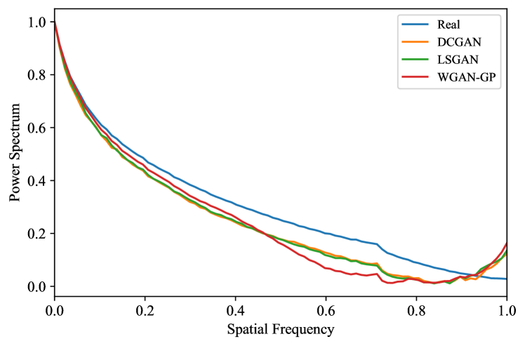
Recent research suggests that CNN-based generation methods are unable to reproduce high frequency distribution of real images. Existing work tends to conclude that this incompetency is an intrinsic property of CNN-based generative models [12, 10, 25]. While Zhang et al.[44] and Wang et al.[42] report that CNN generated images have frequency artifacts, Dzanic et al.[12] and Durall et al.[10] suggest spectrum discrepancies in high frequency: CNN-generated images at the highest frequencies do not decay as usually observed in real images (Figure 1). In particular,
-
•
Dzanic et al.[12] analyze high frequency of real and deep network generated images, and conclude that “deep network generated images share an observable, systematic shortcoming in replicating the attributes of these high-frequency modes”.
-
•
Durall et al.[10] observe that “CNN based generative deep neural networks are failing to reproduce spectral distributions”, and “this effect is independent of the underlying architecture”.
-
•
Dzanic et al.[12] take a step further and propose to exploit this frequency discrepancies for detection of deep network generated images, claiming an accuracy of up to 99.2% across multiple state-of-the-art GAN and VAE models.
Some works also propose different techniques to disguise these high frequency discrepancies via post-processing the deep network generated images [12, 25], or modifying the GAN training objective to avoid these discrepancies [10].
It should be noted that the cause of this discrepancy111The terms spectral discrepancies and spectral inconsistency are used invariably where we refer to high frequency spectral decay discrepancies. We also use the terms CNN-generated and synthetic invariably. has not been agreed upon. Zhang et al.[44] and Durall et al.[10] suggest that this discrepancy could be caused by transposed convolution. As transposed convolution is used throughout the generator architectures, it is difficult to replace them. Therefore, Durall et al.[10] propose spectral regularization to counteract this throughout the GAN training. Meanwhile, Dzanic et al.[12] attribute this discrepancy to the linear dependencies in the spectrum of convolutional filters [25], which hinder learning of high frequencies.
 |
 |
1.2 CNN-generated Image Detectors
Many works have addressed the possibilities of creating detectors to identify synthetic images apart from real images. Though synthetic image detectors (CNN-based) worked reasonably with RGB inputs [42, 5], with spectral discrepancies being observed, several works have proposed to use the corresponding Fourier representation to train these detectors [44, 13]. In particular, Frank et al.[13] showed that detectors using frequency domain yielded better results compared to using the RGB counterpart.
Though observations corresponding to distinguishable frequency footprints being left by CNN-generated images remained mostly qualitative, Dzanic et al.[12] and Durall et al.[10, 11] studied the spectral decay attributes and quantified this behaviour via averaging the power spectrum over frequencies radially to represent them as 1D information. Through this, they observed high frequency spectral decay inconsistencies in CNN-generated images. Furthermore, Dzanic et al.[12] proposed to use a simple KNN classifier using high frequency spectral attributes (3 features extracted per image) that surprisingly obtained very high accuracy in identifying synthetic images only with very small amount of training data. Similarly, Durall et al.[11] used the entire 1d-power spectrum (contains all frequency information) as features to perform detection using Logistic regression, SVM and K-means clustering algorithms. These detectors [12, 11] rely on the belief that high frequency decay discrepancies are intrinsic in CNN-generated images.
1.3 Our contributions
In this work, we take a closer look at the high frequency decay discrepancies in CNN-generated images. Analysis of CNN-generated images is a daunting task: a large number of different architectures, algorithms and objective functions have been proposed to train generators. Instead, our study focuses on the last layer of the generators. Our justification is as follows. Based on Sampling Theorem [20], the frequency contents of the outputs of individual layers are limited by the sampling resolution of the corresponding outputs. As previous work has reported the discrepancies between real and CNN-generated images at the highest frequencies, we hypothesize that inner generator layers (which produce lower resolution outputs) are not directly responsible for the high frequency discrepancies. Therefore, we focus on the last upsampling layer of generative CNN models.
Due to our focus being localized at the last layer, we are able to pinpoint the component that is related to this discrepancy across multiple GAN loss functions, architectures, datasets and resolutions. Our candidate GANs are similar to Durall et al.[10]: DCGAN [34], LSGAN [31], WGAN-GP [17] and we also extend to StarGAN [7]. Our experiments suggest that the frequency discrepancies can be largely avoided by simply modifying the feature map scaling of the last layer. Importantly, using the same training algorithms, objective functions and network architectures (except using a different scaling in the last layer) as in standard GAN models, we are able to avoid the spectral discrepancies. Therefore, our work provides counterexamples to argue that high frequency discrepancies are not intrinsic for CNN-generated images. Furthermore, we are able to successfully bypass the synthetic image detector proposed by Dzanic et al.[12] with only such change in the last scaling step, showing that such approach may not be reliable for detection of deep network generated images. The key takeaway from our work is:
-
•
High frequency spectral decay discrepancies are not intrinsic for CNN-generated images. Therefore, we urge re-thinking in using such features for CNN-generated image detection.
2 Related Work
Dzanic et al.[12] show that CNN-generated images (GANs and VAEs) demonstrate different Fourier spectrum decay characteristics. Since the spectra of natural images tend to behave following the power law [41], Dzanic et al.[12] show that the Fourier modes of deep network generated images at the highest frequencies did not decay as seen in real images, but instead stayed approximately constant. Furthermore, they propose to exploit these discrepancies to detect CNN-generated synthetic images by fitting a decay function to the reduced spectra, and using the parameters of the fitted decay function to build a simple kNN classifier.
Durall et al.[10] show that popular GAN image generators fail to approximate the spectral distributions of real data, and they attribute this to the use of transpose convolutions for upsampling. They show that this effect is independent of the underlying architecture using 1-dimensional spectral characteristics of images generated from DCGAN [34], LSGAN [31], WGAN-GP[17] and DRAGAN [26]. Since transpose convolutions are used in the entire generator models, the propose to counteract their effects by adding a spectral regularization term to the Generator, thereby penalizing the generator for spectral distorted samples.
Khayatkhoei and Elgammal [25] suggest the presence of a systematic bias in GANs against learning high frequencies. They specifically show that for a given kernel size, as resolution increases, the correlation/ dependency of the kernel’s spectrum increases thereby systematically preventing GANs to learn high frequencies without affecting the adjacent frequencies. To alleviate this shortcoming, they propose frequency shifted generators whose frequencies are shifted towards specific high frequencies.
3 Background
The 2D discrete Fourier transform of a 2D image can be written as,
| (1) |
for , . We follow the convention in [12, 10] and compute the azimuthally average of the magnitude of Fourier coefficients over radial frequencies to obtain the reduced spectrum and normalize it. The reduced spectra indicates the strength of the signal with respect to different spatial frequencies. Since our study focuses on high frequency Fourier attributes, we pay attention to the last of the spatial frequencies (0.75 - 1.0 normalized spatial frequencies) similar to [12].
The Sampling Theorem ([20], chapter 4.2) states that: A bandlimited image with bandwidths can be recovered without error from the sample values provided the sampling rate is greater than the Nyquist rate: . The image with bandwidths means that there is no frequency content outside a bounded region in the frequency plane defined by . Details and mathematical proofs can be found in [20] chapter 4.2.
4 Last Upsampling Operation and Fourier Discrepancies
Based on last section, the maximum frequency represented by a discrete 2D signal is constrained by the spatial resolution (sampling) of the signal. Previous work has consistently reported discrepancies in the highest frequencies [10, 12]. Therefore, we hypothesize that inner generator layers that produce lower resolution outputs may not be directly responsible for the high frequency discrepancies. Therefore, we focus on the last upsampling step. In particular, we split the last step into 2 operations, 1) Feature map scaling and 2) Convolution.
4.1 Feature Map Scaling
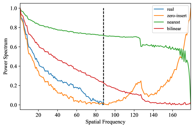
Feature map scaling is a non-parametric operation that scales the input in both dimensions by some factor (Usually 2 in most GAN architectures). In this work, we focus on 3 common feature map scaling techniques. 1) Zero-insert scaling inserts zero between every row and column, scaling the input in both dimensions which is also used by transpose convolutions. 2) Nearest interpolation scales the input by inserting nearest neighbour values. 3) Bilinear interpolation scales the input by inserts new values by taking the weighted average of adjacent values.
From frequency perspective, zero-insertion introduces the largest amount of high frequency content as it replicates the low frequency spectrum for the high frequencies [44], followed by billinear and nearest interpolation. We focus more on the “spectral trend” than the frequency values, and show a schematic example of these upsampling effects on the normalized reduced spectra in Figure 2 by upsampling a reference image of 128x128 from CelebA. [29]
4.2 Convolution
The subsequent convolution operation learns kernels in order to satisfy the optimization objective. Convolutional kernels are capable of suppressing/ amplifying high frequencies. \egA Gaussian kernel suppresses high frequencies and a bilateral kernel amplifies high frequencies. So when designing upsampling blocks in GANs, the general intuition is that irrespective of the feature map scaling method, the kernels will learn to manipulate the scaled feature maps to satisfy the objective function.
5 Experiments
Here we discuss the main experiments. Additional experiments and analysis can be found in Supplementary.
In order to investigate the effects of these 2 operations, we design a rigorous test bed that can address feature map scaling, kernel size and number of kernels independently. Our aim is to isolate the effects of these 2 operations and understand their roles (if any) in causing the high frequencies discrepancies. We use celebA [29] dataset at 128x128 resolution and use 3 GANs with identical architectures but different loss functions namely 1) DCGAN [34], 2) LSGAN [31] and 3) WGAN-GP [17]. All baseline models consist of transpose convolutions with kernel size 4 identical to most out of the box GAN architectures including CycleGAN [46], StarGAN [7] and VQ-VAE [40].
Proposed Test Bed. Table 1 summarizes our test bed. All baseline experiments using transpose convolutions of kernel size 4 are indicated by the experiment code Baseline and our handcrafted experiments are indicated using the 3 character code: An experiment code of X.Y.Z indicates X type of feature map scaling (Possible values are Z : Zero-insertion, N: Nearest interpolation, B: Bilinear interpolation), Y number of convolutional blocks and Z sized convolutional kernels for the last upsampling step. \egA code of N.1.5 indicates nearest interpolation feature map scaling with a single convolutional block of 5x5 kernel for the last upsampling step. Note that we focus on up scaling by a factor of 2 as used in most GAN models. Our test bed summary is shown in table 1 and it contains experiments addressing the following factors:
Feature Map scaling. In order to investigate the effect of feature map scaling on high frequency Fourier attributes, we use experiments Z.1.5, N.1.5 and B.1.5. We explicitly conduct experiments using zero-insert feature map scaling as sanity check experiments to verify the effects of transpose convolutions. Do note that we had to use odd size kernel to maintain the spatial size after scaling, and hence we use kernels of size 5 for the last convolutional block.
Kernel Size. We use experiments x.1.3, x.1.5 and x.1.7 to investigate the kernel size effects on high frequency Fourier behaviour. Here x refers to Z, N or B for different types of scaling as discussed.
Number of kernels. Further, we use experiments x.1.5 and x.3.5 to study the effect of number of kernels on the high frequency Fourier behaviour.
Code Details Baseline Transpose convolution (4x4 kernel) N.1.5 Nearest Upsampling + 1 conv block of 5x5 kernel Z.1.5 Zero insert Upsampling + 1 conv block of 5x5 kernel B.1.5 Bilinear Upsampling + 1 conv block of 5x5 kernel N.1.3 Nearest Upsampling + 1 conv block of 3x3 kernel N.1.7 Nearest Upsampling + 1 conv block of 7x7 kernel Z.1.3 Zero insert Upsampling + 1 conv block of 3x3 kernel Z.1.7 Zero insert Upsampling + 1 conv block of 7x7 kernel B.1.3 Bilinear Upsampling + 1 conv block of 3x3 kernel B.1.7 Bilinear Upsampling + 1 conv block of 7x7 kernel N.3.5 Nearest Upsampling + 3 conv blocks of 5x5 kernel Z.3.5 Zero insert upsampling + 3 conv blocks of 5x5 kernel B.3.5 Bilinear upsampling + 3 conv blocks of 5x5 kernel
6 Metrics
Spectral behaviour of synthetic images have been analysed only qualitatively, not quantitatively in previous works [12, 10, 11]. Defining a spectral consistency metric is non-trivial and to be consistent, we will qualitatively analyse the high frequency spectral distribution in our experiments. Synthetic images are spectral consistent if they demonstrate power spectrum decay behaviour similar to their training data, and if not, vice versa. We use 4000 real and GAN images to generate spectral distribution curves. To ensure that our setups were trained properly, we use FID scores to assess the quality of samples and make sure that they are consistent with the FID scores from baseline experiments.
7 Results
7.1 Effect of Feature Map Scaling Methods
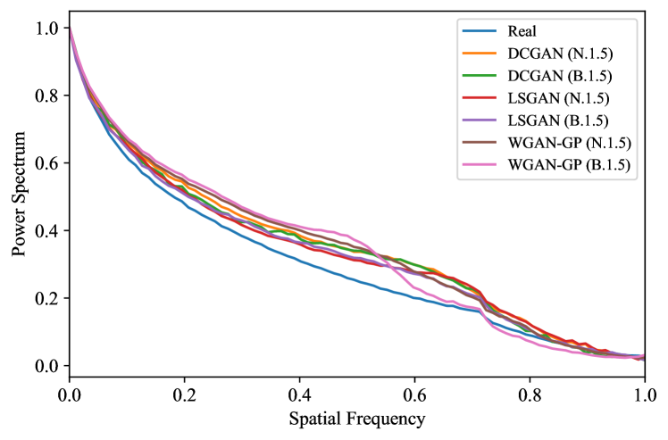
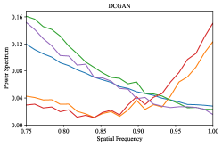
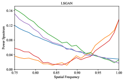
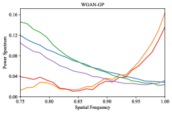
Figure 3 illustrates the resulting spectral distributions when using different feature map scaling methods. We observe that images from Z.1.5 and Baseline experiments are spectral inconsistent for all 3 GANs. Nearest and bilinear interpolation methods are able to replicate the spectral distribution of real data reasonably across all 3 GAN models. Since the only change in our models is the feature map scaling method in the last layer while the algorithms, objective functions and majority of the network architectures are identical to public released code, these results qualify to support our thesis that high frequency Fourier discrepancies are not inherent to GANs.
 |
 |
 |
7.2 Effect of Kernel Size
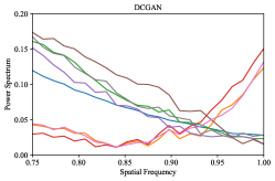
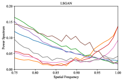
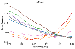
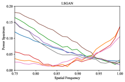
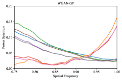
From Figure 4, we observe that smaller kernel sizes result in more turbulent spectral behaviour for N.1.3 and B.1.3 LSGAN experiments. Apart from this observation, experiments using nearest and bilinear interpolation methods are able to reproduce spectral distributions of real data reasonably well, and zero-insertion based methods always result in high frequency spectral distortions. Further, from Figure 5, we observe that when using larger kernels, all experiments using nearest and bilinear interpolation methods are able to replicate spectral behaviour of real data, and even with larger kernels zero-insertion based methods produce high frequency spectral distortions (Z.1.7).
 |
 |
 |
 |
 |
 |
7.3 Effect of Number of Kernels
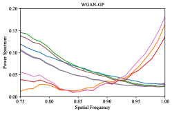
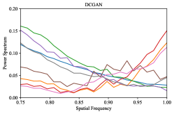
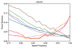
Figure 6 illustrates that increasing the number of kernels do not yield spectral consistency by itself. Apart from N.3.5 DCGAN experiment, we observe that all other experiments using nearest and bilinear interpolation methods are able to approximate the spectral behaviour of real data. Also, GAN objective functions do not impose any spectral requirements. Thus the kernels do not have any direct incentive for imposing spectral consistency.
 |
 |
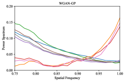 |
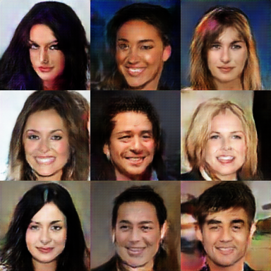
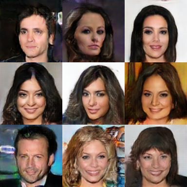
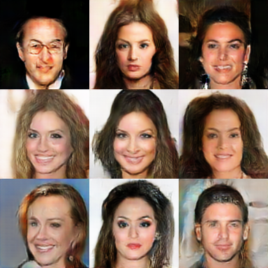
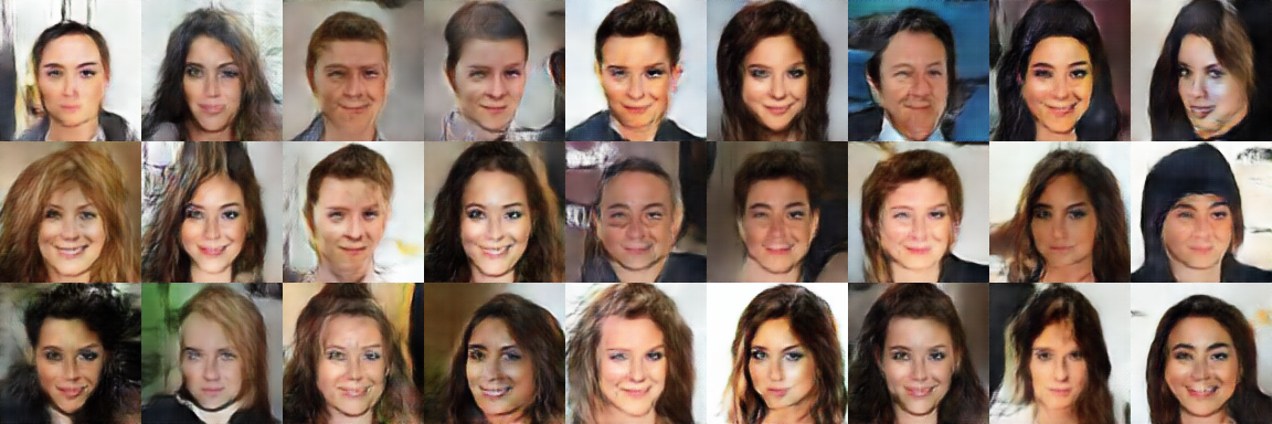
Key observations. Throughout all 39 rigorous experiments, we observe that zero insertion based feature map scaling methods (including Baseline) are consistently showing high frequency spectral discrepancies, and most experiments (22/24) using bilinear and nearest interpolation methods are able to avoid these high frequency spectral discrepancies. All these results support our statement that high frequency spectral discrepancies are not inherent characteristics to GANs. The FID scores for all experiments were comparable with the baseline FID, and are included in the Supplementary E. We show image samples from WGAN-GP for Baseline, N.1.5 and B.1.5 setups in Figure 7. Do note that for all experiments, we use the exact same discriminator architecture as the Baseline experiment.
8 Fourier Synthetic Image Detector
Dzanic et al.[12] state that the spectral properties of real and deep network generated images are fundamentally different, and proposed a synthetic image detection method using a “simple” k-nearest neighbours (KNN) classifier to emphasize the extent of these spectral differences. We follow the exact procedure as the original authors to train these classifiers and details can be found in Supplementary F.1.
8.1 Experiment Setup
With nearest and bilinear interpolation methods obtaining spectral consistent GANs for the previous experiments, we question whether the classifier proposed above would be robust enough to detect these samples as fake. To investigate this we follow the following steps:
-
1.
We train 3 KNN classifiers, one for DCGAN, LSGAN and WGAN-GP respectively. For GAN images, we use images generated from the Baseline experiment (using transpose convolutions) as training data.
-
2.
We test these classifiers using GAN images generated from the setups in our test bed to evaluate the robustness of the classifier.
-
3.
We also repeat the experiments using 50% data for training the classifier (The original work used only 10%) to observe any improvements in accuracy.
8.2 Detection Results
The complete detection results are shown in table 2. We observe that all setups corresponding to N.x.x and B.x.x experiments are able to easily bypass the classifier. Even when 50% training data is used, we are able to bypass the classifier with ease (Included in Supplementary F.2). The results clearly demonstrate that the proposed classifier relying on high frequency Fourier attributes to detect synthetic images, fails to detect images generated from identical GAN models with last feature map scaling replaced by nearest or bilinear interpolation methods. These results are consistent with the observed spectral distributions. By combining these detection results with the empirical finding that high frequency spectral discrepancies are not inherent characteristics of CNN-generated images, we suggest re-thinking of using such discrepancies to detect synthetic images.
Setup DCGAN LSGAN WGAN-GP N.1.5 % % % Z.1.5 % % % B.1.5 % % % N.1.3 % % % N.1.7 % % % Z.1.3 % % % Z.1.7 % % % B.1.3 % % % B.1.7 % % % N.3.5 % % % Z.3.5 % % % B.3.5 % % %
9 Extended experiments
With observations that high frequency Fourier spectrum discrepancies are not intrinsic characteristics of GANs, we extend our experiments to address different dataset, image resolution and GAN objective function to further find evidences to support our thesis statement. We select 3 setups from our test bed Z.1.5, N.1.5 and B.1.5 to conduct extended experiments since we have observed that kernel size/ number of kernels do not substantially manipulate high frequencies compared to feature map scaling methods. Similar to previous experiments, we analyze the resulting spectral distributions and evaluate the robustness of the synthetic detector proposed by Dzanic et al.[12].
9.1 LSUN Bedrooms Dataset
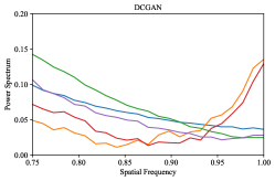
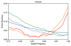
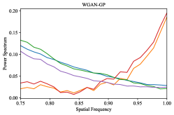
In this experiment we use a subset of LSUN Bedrooms Dataset [43] (128x128) to train DCGAN [34], LSGAN [31] and WGAN-GP [17] identical to previous setups. The spectral plots are shown in Figure 8. We observe identical results to CelebA experiment (Figure 3). That is we observe N.1.5 and B.1.5 are producing spectral consistent GANs and this further supports our statement that high frequency spectral discrepancies are not inherent in GANs. We also evaluate the synthetic image detector and observe that N.1.5 and B.1.5 samples can easily bypass the detector. (See table 3)
 |
 |
 |
Setup DCGAN LSGAN WGAN-GP N.1.5 Z.1.5 % % % B.1.5
| Setup | N.1.5 | Z.1.5 | B.1.5 |
|---|---|---|---|
| Accuracy | % | % |
9.2 Image-to-Image Translation
We extend our experiments to Image-to-Image translation domain using StarGAN [7]. Here we use resized CelebA [29] (256x256) used by the official StarGAN [7] implementation to study whether spectral consistency can be achieved by modifying the last feature map scaling operation. We train StarGANs for Z.1.5, N.1.5 and B.1.5 setups. The spectral plots are shown in Figure 9. We observe that only B.1.5 is able to produce spectral consistent GANs and N.1.5 produces high frequency Fourier discrepancies. We would not ask ourselves why nearest interpolation method behaves differently than bilinear, but rather confirm that we are able to find bilinear interpolation results as more evidence to support our statement that high frequency spectral discrepancies are not inherent characteristics to GANs. We further evaluate the synthetic image detector and observe that B.1.5 samples can bypass the classifier. (See table 4)
10 Spectral Regularization
The recent Spectral regularization (SR) by Durall et al.[10] proposed to add a regularizer term to the generator loss to explicitly penalize the generator for spectral distortions. Using SR, they were able to obtain spectral consistency for DCGAN [34], LSGAN [31], WGAN-GP [17] and DRAGAN [26] using the celebA [29] (128x128). This method encounters computational overhead due to calculation of reduced spectrum for images during training. We show that by modifying the last feature map scaling operation, we are able to achieve spectral consistent GANs without SR. Importantly, we show that no change in objective functions is needed. These results and more discussion on SR can be found in Supplementary B.
11 Discussion
In this study, we investigated the validity of contemporary beliefs that CNN-based generative models are unable to reproduce high frequency decay attributes of real images. We employ a systematic study to design counterexamples to challenge the existing beliefs. With maximum frequency bounded by the spatial resolution, and Fourier discrepancies reported at the highest frequencies, we hypothesized that the last upsampling operation is mostly related to this shortcoming. With carefully designed experiments spanning multiple GAN architectures, loss functions, datasets and resolutions, we observe that high frequency spectral decay discrepancies can be avoided by replacing zero insertion based scaling used by transpose convolutions with nearest or bilinear at the last step. Note that we do not claim that modifying the last feature map scaling method will always fix spectral decay discrepancies in every situation, but rather the goal of our study is to provide counterexamples to argue that high frequency spectral decay discrepancies are not inherent characteristics of CNN-generated images. Further, we easily bypass the recently proposed synthetic image detector that exploits this discrepancy information to detect CNN-generated images indicating that such features are not robust for the purposes of synthetic image detection.
In Supplementary material, we provide more GAN models [6, 28] with no high frequency decay discrepancies. We also investigate whether such high frequency decay discrepancies are found in other types of computational image synthesis methods (synthesis using Unity game engine222https://unity.com/) [15, 14]. To conclude, through this work we hope to help image forensics research manoeuvre in more plausible directions to combat the fight against CNN-synthesized visual disinformation.

Acknowledgments: This project was supported by SUTD project PIE-SGP-AI-2018-01. This research was also supported by the National Research Foundation Singapore under its AI Singapore Programme [Award Number: AISG-100E2018-005]. This work was also supported by ST Electronics and the National Research Foundation (NRF), Prime Minister’s Office, Singapore under Corporate Laboratory @ University Scheme (Programme Title: STEE Infosec - SUTD Corporate Laboratory).
We also gratefully acknowledge the support of NVIDIA AI Technology Center (NVAITC) for our research.
References
- [1] Martin Arjovsky, Soumith Chintala, and Léon Bottou. Wasserstein gan, 2017.
- [2] Paul Baines. Uk election 2019: after fake keir starmer clip, how much of a problem are doctored videos?, Aug 2020.
- [3] Andrew Brock, Jeff Donahue, and Karen Simonyan. Large scale GAN training for high fidelity natural image synthesis. In International Conference on Learning Representations, 2019.
- [4] Andrew Brock, Jeff Donahue, and Karen Simonyan. Large scale gan training for high fidelity natural image synthesis, 2019.
- [5] Lucy Chai, David Bau, Ser-Nam Lim, and Phillip Isola. What makes fake images detectable? understanding properties that generalize. In Andrea Vedaldi, Horst Bischof, Thomas Brox, and Jan-Michael Frahm, editors, Computer Vision – ECCV 2020, pages 103–120, Cham, 2020. Springer International Publishing.
- [6] Qifeng Chen and V. Koltun. Photographic image synthesis with cascaded refinement networks. 2017 IEEE International Conference on Computer Vision (ICCV), pages 1520–1529, 2017.
- [7] Yunjey Choi, Minje Choi, Munyoung Kim, Jung-Woo Ha, Sunghun Kim, and Jaegul Choo. Stargan: Unified generative adversarial networks for multi-domain image-to-image translation. In Proceedings of the IEEE Conference on Computer Vision and Pattern Recognition, 2018.
- [8] Yunjey Choi, Youngjung Uh, Jaejun Yoo, and Jung-Woo Ha. Stargan v2: Diverse image synthesis for multiple domains. In Proceedings of the IEEE/CVF Conference on Computer Vision and Pattern Recognition (CVPR), June 2020.
- [9] Danielle Citron and Robert Chesney. Deepfakes and the new disinformation war, Jun 2020.
- [10] Ricard Durall, Margret Keuper, and Janis Keuper. Watch your up-convolution: Cnn based generative deep neural networks are failing to reproduce spectral distributions. In IEEE/CVF Conference on Computer Vision and Pattern Recognition (CVPR), June 2020.
- [11] Ricard Durall, Margret Keuper, Franz-Josef Pfreundt, and Janis Keuper. Unmasking deepfakes with simple features, 2020.
- [12] Tarik Dzanic, Karan Shah, and Freddie Witherden. Fourier spectrum discrepancies in deep network generated images. In Thirty-fourth Annual Conference on Neural Information Processing Systems (NeurIPS), December 2020.
- [13] Joel Frank, Thorsten Eisenhofer, Lea Schönherr, Asja Fischer, Dorothea Kolossa, and Thorsten Holz. Leveraging frequency analysis for deep fake image recognition. In Hal Daumé III and Aarti Singh, editors, Proceedings of the 37th International Conference on Machine Learning, volume 119 of Proceedings of Machine Learning Research, pages 3247–3258. PMLR, 13–18 Jul 2020.
- [14] A. Gaidon, Q. Wang, Y. Cabon, and E. Vig. Virtualworlds as proxy for multi-object tracking analysis. In 2016 IEEE Conference on Computer Vision and Pattern Recognition (CVPR), pages 4340–4349, 2016.
- [15] Andreas Geiger, Philip Lenz, and Raquel Urtasun. Are we ready for autonomous driving? the kitti vision benchmark suite. In Conference on Computer Vision and Pattern Recognition (CVPR), 2012.
- [16] Ian Goodfellow, Jean Pouget-Abadie, Mehdi Mirza, Bing Xu, David Warde-Farley, Sherjil Ozair, Aaron Courville, and Yoshua Bengio. Generative adversarial nets. In Z. Ghahramani, M. Welling, C. Cortes, N. Lawrence, and K. Q. Weinberger, editors, Advances in Neural Information Processing Systems, volume 27, pages 2672–2680. Curran Associates, Inc., 2014.
- [17] Ishaan Gulrajani, Faruk Ahmed, Martin Arjovsky, Vincent Dumoulin, and Aaron C Courville. Improved training of wasserstein gans. In I. Guyon, U. V. Luxburg, S. Bengio, H. Wallach, R. Fergus, S. Vishwanathan, and R. Garnett, editors, Advances in Neural Information Processing Systems, volume 30, pages 5767–5777. Curran Associates, Inc., 2017.
- [18] Karen Hao and Will Douglas Heaven. The year deepfakes went mainstream, Dec 2020.
- [19] Ellie Harrison. Shockingly realistic tom cruise deepfakes go viral on tiktok, Feb 2021.
- [20] Anil K. Jain. Fundamentals of Digital Image Processing. Prentice-Hall, Inc., USA, 1989.
- [21] Tero Karras, Timo Aila, Samuli Laine, and Jaakko Lehtinen. Progressive growing of GANs for improved quality, stability, and variation. In International Conference on Learning Representations, 2018.
- [22] Tero Karras, Miika Aittala, Janne Hellsten, Samuli Laine, Jaakko Lehtinen, and Timo Aila. Training generative adversarial networks with limited data. In H. Larochelle, M. Ranzato, R. Hadsell, M. F. Balcan, and H. Lin, editors, Advances in Neural Information Processing Systems, volume 33, pages 12104–12114. Curran Associates, Inc., 2020.
- [23] Tero Karras, Samuli Laine, and Timo Aila. A style-based generator architecture for generative adversarial networks. In Proceedings of the IEEE/CVF Conference on Computer Vision and Pattern Recognition (CVPR), June 2019.
- [24] Tero Karras, Samuli Laine, Miika Aittala, Janne Hellsten, Jaakko Lehtinen, and Timo Aila. Analyzing and improving the image quality of stylegan. In Proceedings of the IEEE/CVF Conference on Computer Vision and Pattern Recognition (CVPR), June 2020.
- [25] Mahyar Khayatkhoei and Ahmed Elgammal. Spatial frequency bias in convolutional generative adversarial networks, Oct 2020.
- [26] Naveen Kodali, Jacob Abernethy, James Hays, and Zsolt Kira. On convergence and stability of gans, 2017.
- [27] C. Ledig, L. Theis, F. Huszár, J. Caballero, A. Cunningham, A. Acosta, A. Aitken, A. Tejani, J. Totz, Z. Wang, and W. Shi. Photo-realistic single image super-resolution using a generative adversarial network. In 2017 IEEE Conference on Computer Vision and Pattern Recognition (CVPR), pages 105–114, 2017.
- [28] K. Li, T. Zhang, and J. Malik. Diverse image synthesis from semantic layouts via conditional imle. In 2019 IEEE/CVF International Conference on Computer Vision (ICCV), pages 4219–4228, 2019.
- [29] Ziwei Liu, Ping Luo, Xiaogang Wang, and Xiaoou Tang. Deep learning face attributes in the wild. In Proceedings of International Conference on Computer Vision (ICCV), December 2015.
- [30] Sophie Maddocks. ‘a deepfake porn plot intended to silence me’: exploring continuities between pornographic and ‘political’ deep fakes. Porn Studies, 0(0):1–9, 2020.
- [31] X. Mao, Q. Li, H. Xie, R. Y. K. Lau, Z. Wang, and S. P. Smolley. Least squares generative adversarial networks. In 2017 IEEE International Conference on Computer Vision (ICCV), pages 2813–2821, 2017.
- [32] Rachel Metz. The number of deepfake videos online is spiking. most are porn, Oct 2019.
- [33] Taesung Park, Ming-Yu Liu, Ting-Chun Wang, and Jun-Yan Zhu. Semantic image synthesis with spatially-adaptive normalization. In Proceedings of the IEEE/CVF Conference on Computer Vision and Pattern Recognition (CVPR), June 2019.
- [34] Alec Radford, Luke Metz, and Soumith Chintala. Unsupervised representation learning with deep convolutional generative adversarial networks, 2016.
- [35] Ali Razavi, Aaron van den Oord, and Oriol Vinyals. Generating diverse high-fidelity images with vq-vae-2. In H. Wallach, H. Larochelle, A. Beygelzimer, F. d'Alché-Buc, E. Fox, and R. Garnett, editors, Advances in Neural Information Processing Systems, volume 32, pages 14866–14876. Curran Associates, Inc., 2019.
- [36] Tom Simonite. What happened to the deepfake threat to the election?, Nov 2020.
- [37] Daniel Thomas. Deepfakes: A threat to democracy or just a bit of fun?, Jan 2020.
- [38] Ngoc-Trung Tran, Tuan-Anh Bui, and N. Cheung. Dist-gan: An improved gan using distance constraints. In ECCV, 2018.
- [39] Ngoc-Trung Tran, Viet-Hung Tran, Bao-Ngoc Nguyen, Linxiao Yang, and Ngai-Man (Man) Cheung. Self-supervised gan: Analysis and improvement with multi-class minimax game. In H. Wallach, H. Larochelle, A. Beygelzimer, F. d'Alché-Buc, E. Fox, and R. Garnett, editors, Advances in Neural Information Processing Systems, volume 32. Curran Associates, Inc., 2019.
- [40] Aaron van den Oord, Oriol Vinyals, and koray kavukcuoglu. Neural discrete representation learning. In I. Guyon, U. V. Luxburg, S. Bengio, H. Wallach, R. Fergus, S. Vishwanathan, and R. Garnett, editors, Advances in Neural Information Processing Systems, volume 30, pages 6306–6315. Curran Associates, Inc., 2017.
- [41] A. van der Schaaf and J.H. van Hateren. Modelling the power spectra of natural images: Statistics and information. Vision Research, 36(17):2759 – 2770, 1996.
- [42] Sheng-Yu Wang, Oliver Wang, Richard Zhang, Andrew Owens, and Alexei A. Efros. Cnn-generated images are surprisingly easy to spot… for now. In IEEE/CVF Conference on Computer Vision and Pattern Recognition (CVPR), June 2020.
- [43] Fisher Yu, Yinda Zhang, Shuran Song, Ari Seff, and Jianxiong Xiao. Lsun: Construction of a large-scale image dataset using deep learning with humans in the loop. arXiv preprint arXiv:1506.03365, 2015.
- [44] X. Zhang, S. Karaman, and S. Chang. Detecting and simulating artifacts in gan fake images. In 2019 IEEE International Workshop on Information Forensics and Security (WIFS), pages 1–6, 2019.
- [45] Shengyu Zhao, Zhijian Liu, Ji Lin, Jun-Yan Zhu, and Song Han. Differentiable augmentation for data-efficient gan training. In Conference on Neural Information Processing Systems (NeurIPS), 2020.
- [46] Jun-Yan Zhu, Taesung Park, Phillip Isola, and Alexei A Efros. Unpaired image-to-image translation using cycle-consistent adversarial networkss. In Computer Vision (ICCV), 2017 IEEE International Conference on, 2017.
Supplementary materials include research reproducibility details, additional results and more experiments to support our thesis statement.
Supplementary A Standard Deviation of Experiments
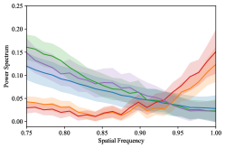
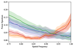
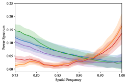
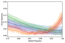
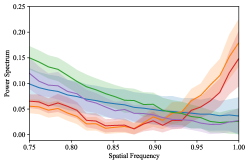
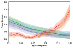
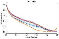
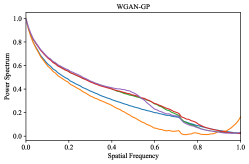
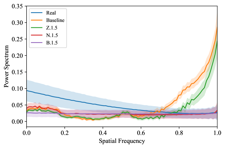
Standard deviation of spectral distributions were not included in the paper to allow better readability of graphs. In this section, we include the standard deviation of experiments for Baseline, Z.1.5, N.1.5 and B.1.5 experiments. The spectral distributions with standard deviations for CelebA [29], LSUN [43] and StarGAN [7] experiments are shown in Figures 10, 11 and 21 respectively. We also show the Standard deviations of Spectral regularization experiments in Figure 12. In all cases, we observe that the standard deviations are within acceptable range.
 |
 |
 |
 |
 |
 |
 |
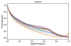 |
 |
Supplementary B Spectral Regularization
Results of SR experiments are shown in Figure 13. More specifically, SR performs generator loss scaling as there are no gradients with respect to the power spectrum difference between real and synthetic images. We were intrigued by the question on how generator loss scaling can achieve spectral consistency as claimed by [10] and noticed that the source code uses N.3.5 setup together with SR333https://github.com/cc-hpc-itwm/UpConv. Analysing SR is out of scope for this work, but we have showed that N.3.5 setup (Main paper) is sufficient to achieve spectral consistency in identical setups.
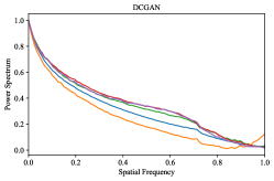 |
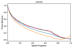 |
 |
Supplementary C Higher Resolution Experiments
In order to further investigate our thesis statement that high frequency decay discrepancies are not inherent characteristics for CNN-generated images, we extend our analysis to larger resolutions. We use image reconstruction as a representative task to investigate these effects at higher resolutions (We use 512x512).
We select a subset of CelebA-HQ [21] dataset to train a standard autoencoder for image reconstruction. Similar to experiments in the paper, we perform experiments corresponding to Baseline, Z.1.5, N.1.5 and B.1.5 setups. We observe that Baseline and Z.1.5 setups produce high frequency Fourier discrepancies for reconstructed images, and N.1.5 and B.1.5 setups produce spectral consistent reconstructed images. The spectral distributions are shown in Figure 14. This further confirms that high frequency Fourier discrepancies are not intrinsic for CNN-generated images.
Supplementary D Samples
We show more samples and spectral distributions for important CelebA [29] experiments in this section.
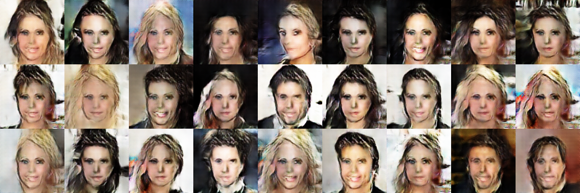
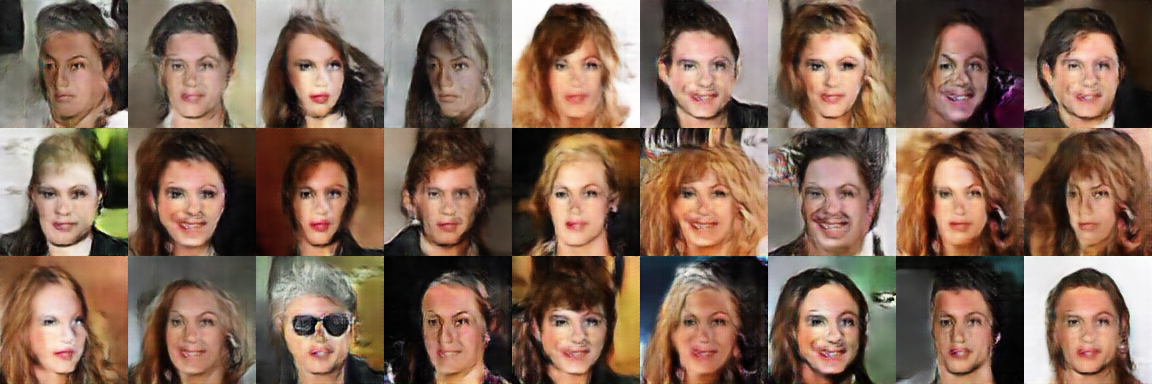
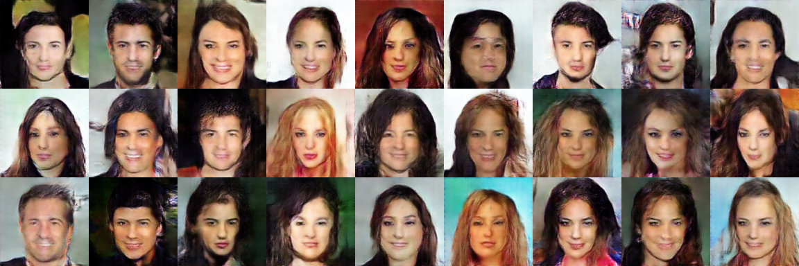
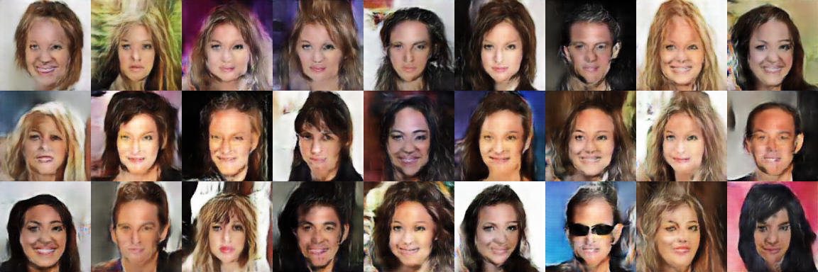
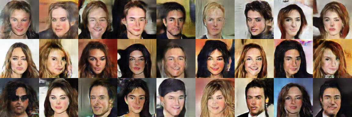
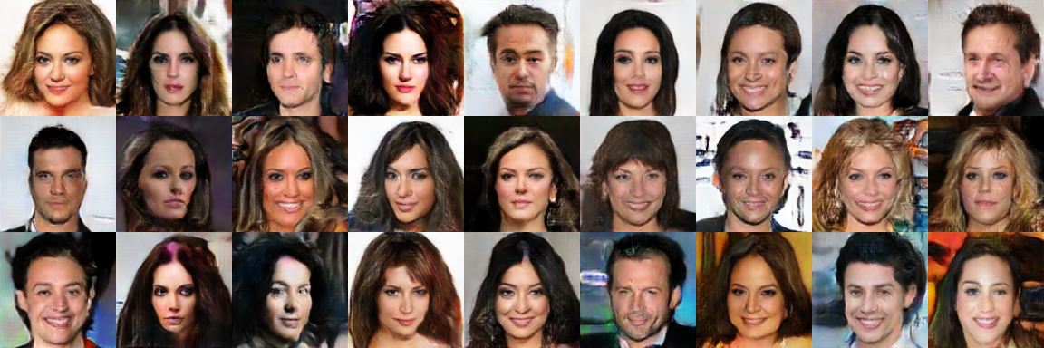
GAN Samples: We show extensive samples corresponding to Baseline, Z.1.5, N.1.5 and B.1.5 setups for DCGAN [34], LSGAN [31], WGAN-GP [17] in Figures 15, 16, 17 respectively.
|
Baseline |
 |
|---|---|
|
Z.1.5 |
 |
|
N.1.5 |
 |
|
B.1.5 |
 |
|
Baseline |
 |
|---|---|
|
Z.1.5 |
 |
|
N.1.5 |
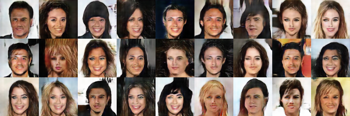 |
|
B.1.5 |
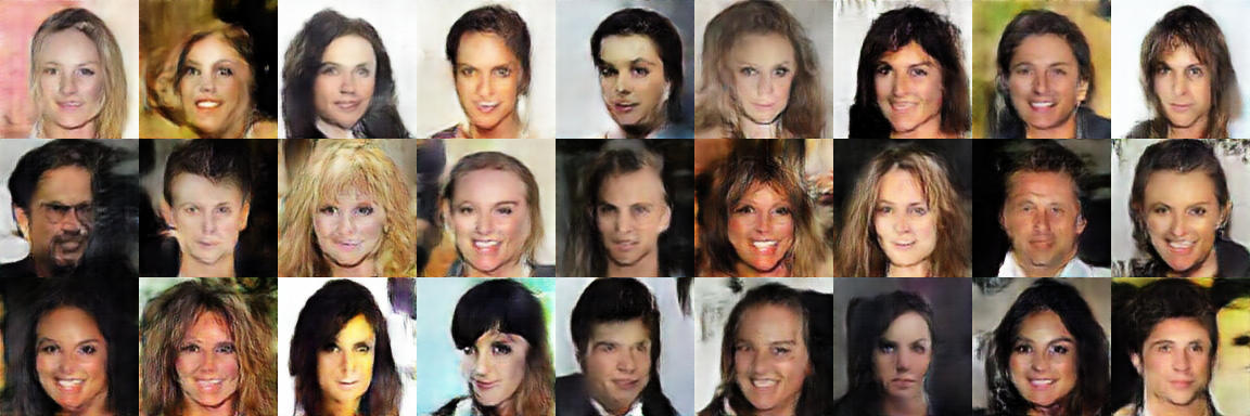 |
|
Baseline |
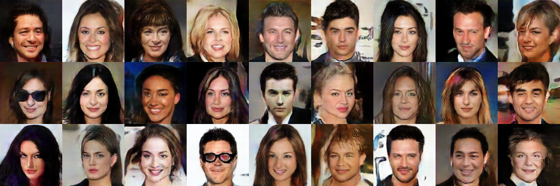 |
|---|---|
|
Z.1.5 |
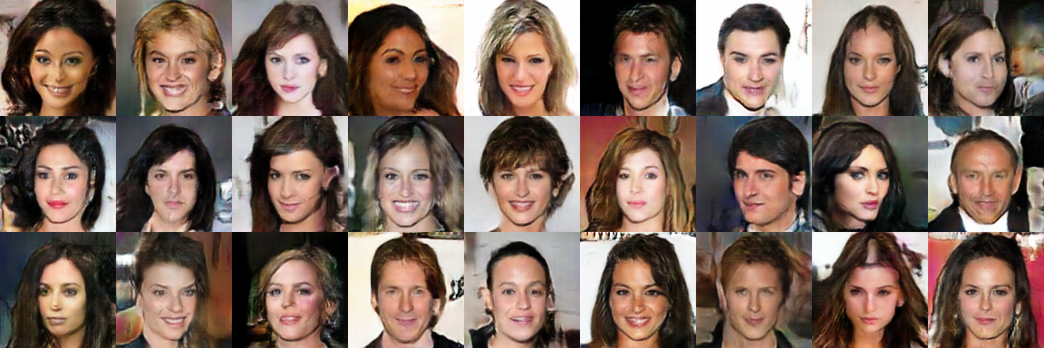 |
|
N.1.5 |
 |
|
B.1.5 |
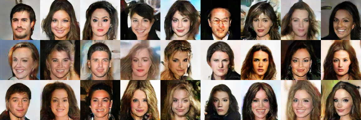 |
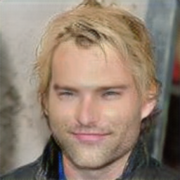
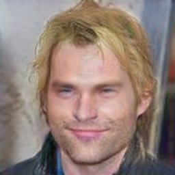
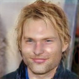
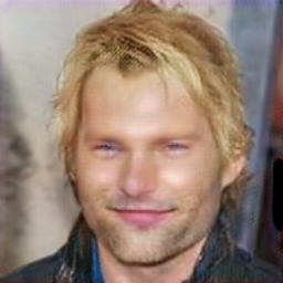
Image-to-Image Translation: For StarGAN [7] experiments, we show an example of a reference image with corresponding translated images for Baseline, Z.1.5, N.1.5 and B.1.5 setups in Figures 18. We show the corresponding spectral distributions in Figure 19.
 |
 |
 |
 |
 |
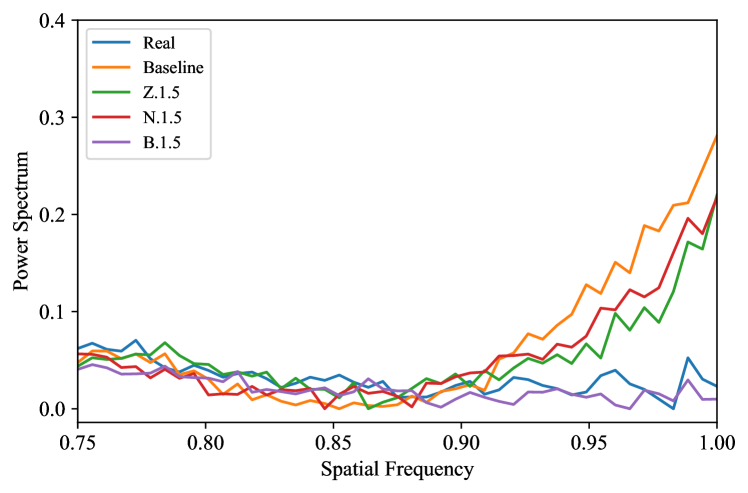 |
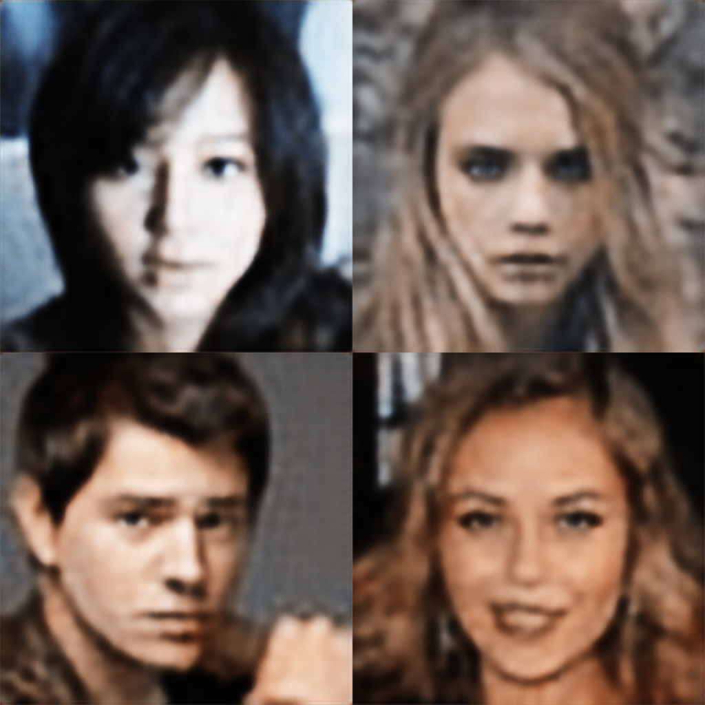
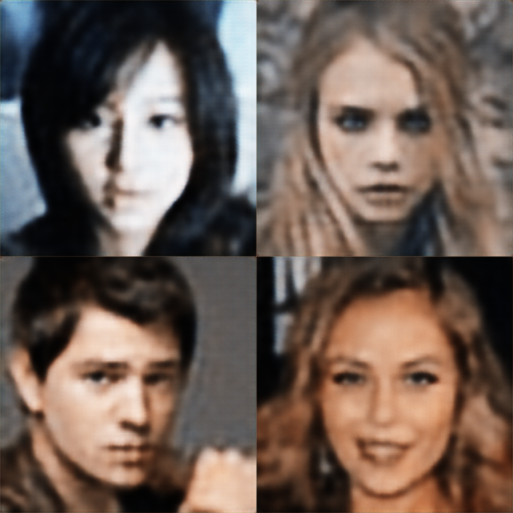
Image Reconstruction: We show image reconstruction results for a few CelebA-HQ [21] examples in Figure 20
 |
 |
 |
 |
 |

Supplementary E FID scores
FID scores for all CelebaA [29] experiments are shown in table 5. We used 50k real images and 50k GAN images to calculate each FID score. We observe that the FID scores of nearest and bilinear interpolation methods are comparable or better than the Baseline FID for all GAN setups.
| Setup Code | DCGAN | LSGAN | WGAN-GP |
|---|---|---|---|
| Baseline | |||
| N.1.5 | |||
| Z.1.5 | |||
| B.1.5 | |||
| N.1.7 | |||
| Z.1.7 | |||
| B.1.7 | |||
| N.1.3 | |||
| Z.1.3 | |||
| B.1.3 | |||
| N.3.5 | |||
| Z.3.5 | |||
| B.3.5 | |||
| SR |
Supplementary F Fourier Synthetic Image Detector
We include more information and results for the synthetic image detector proposed by Dzanic et al.[12]. All detection rates are averaged over 10 independent runs.
F.1 Classifier Implementation Details
The exact procedure used by Dzanic et al.[12] to implement the classifier is shown below. For easier understanding, let us assume that we want to train a classifier to detect between real and StyleGAN images
-
1.
Collect a repository of 1000 StyleGAN images and 1000 real images.
-
2.
Obtain the un-normalized reduced spectrum for every real and StyleGAN image for the last 25% spatial frequencies (0.75 - 1.0).
-
3.
Fit the reduced spectrum using power law function for every real and GAN image.
-
4.
Extract 3 features from the fitted spectrum where : start value of the fitted spectrum, : decay value of the fitted spectrum, : end value of the fitted spectrum. Though the authors mention only in their paper, their official implementation contained as well. This difference is acceptable since is linearly dependent on under the assumption that the power law is a good fit.
-
5.
Train/ apply a binary KNN classifier (with k=5) using the 3 features extracted per image to predict if the GAN images are real or fake. The authors use 100 real and GAN images each to train the classifier and use the remaining 900 samples to test.
F.2 Additional Results
Additional detection results when using 50% data to train (authors used 10% and these results are shown in the main paper) for CelebA [29], LSUN [43] and StarGAN [7] experiments are shown in table 6, 7, 8 respectively. We also conduct experiments using the reconstructed images and the detection results are shown in 9.
Setup DCGAN LSGAN WGAN-GP N.1.5 % % % Z.1.5 % % % B.1.5 % % % N.1.3 % % % N.1.7 % % % Z.1.3 % % % Z.1.7 % % % B.1.3 % % % B.1.7 % % % N.3.5 % % % Z.3.5 % % % B.3.5 % % %
Setup DCGAN LSGAN WGAN-GP N.1.5 Z.1.5 % % % B.1.5
Setup N.1.5 Z.1.5 B.1.5 Accuracy % %
| Setup | 10% train data | 50% train data |
|---|---|---|
| N.1.5 | ||
| Z.1.5 | % | % |
| B.1.5 |
Supplementary G Stronger Classifiers
G.1 SVM and MLP classifiers
We perform additional experiments using SVM and MLP classifiers (exact same setup as [12], only change in classifiers). The results are shown in Table 10 and Table 11. Our results are consistent: even with SVM/MLP classifiers, we can bypass them by replacing zero insertion last layer with nearest (N) or bilinear (B). For all experiments, we use 10% data for training, and the reported results are averaged over 10 runs. We also observe similar detection rates when using 50% and 80% data for training.
Setup DCGAN LSGAN WGAN-GP N.1.5 % % % Z.1.5 % % % B.1.5 % % % N.1.3 % % % N.1.7 % % % Z.1.3 % % % Z.1.7 % % % B.1.3 % % % B.1.7 % % % N.3.5 % % % Z.3.5 % % % B.3.5 % % %
Setup DCGAN LSGAN WGAN-GP N.1.5 % % % Z.1.5 % % % B.1.5 % % % N.1.3 % % % N.1.7 % % % Z.1.3 % % % Z.1.7 % % % B.1.3 % % % B.1.7 % % % N.3.5 % % % Z.3.5 % % % B.3.5 % % %
Setup DCGAN LSGAN WGAN-GP N.1.5 % % % Z.1.5 % % % B.1.5 % % % N.1.3 % % % N.1.7 % % % Z.1.3 % % % Z.1.7 % % % B.1.3 % % % B.1.7 % % % N.3.5 % % % Z.3.5 % % % B.3.5 % % %
G.2 Using entire spectrum as features
We followed similar setup as Durall et al.[10] to train a SVM classifier using entire spectrum as features (88 dimensional features for 128x128 images). The finding is consistent: we observe that the features are still non-separable when using nearest (N) and bilinear (B) for the last upsampling step. The results are shown in Table 12.
Supplementary H Virtual KITTI
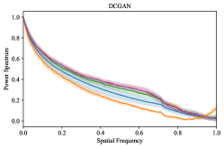
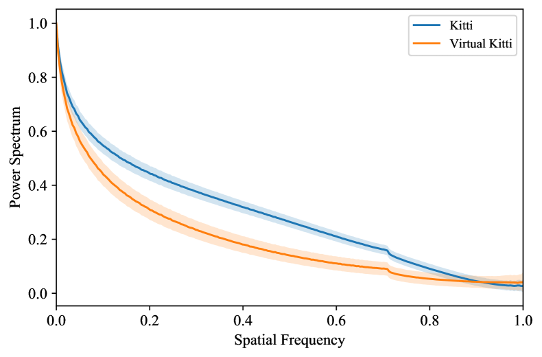
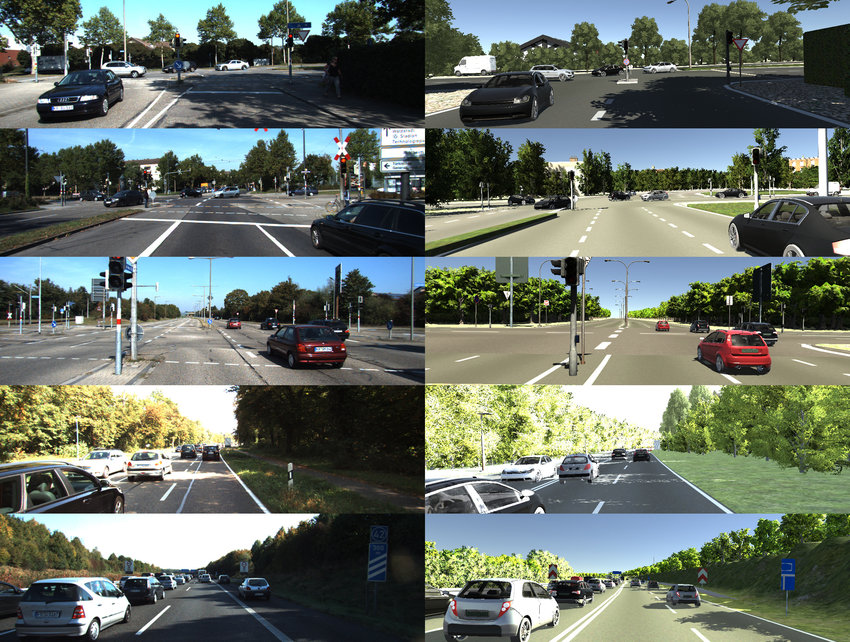
GANs belong to a larger family of computational image synthesis algorithms. In this section, we investigate the high frequency decay attributes of data created entirely using Unity Game Engine. We compare the spectral behaviour between the Official KITTI tracking benchmark [15] (Real images) and the Virtual KITTI [14] (Synthesized images). Virtual KITTI [14] recreates real-world videos from the KITTI tracking benchmark [15] inside Unity444https://unity.com/ game engine. We show some samples in Figure 25. We show the entire power spectrum in Figure 22 and we observe that the images synthesized from the game engine do not have high frequency spectral discrepancies.
Supplementary I CRN/ IMLE
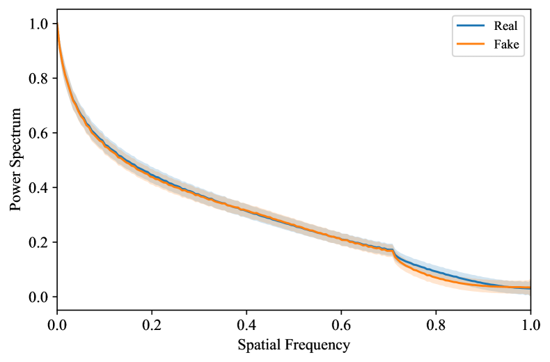
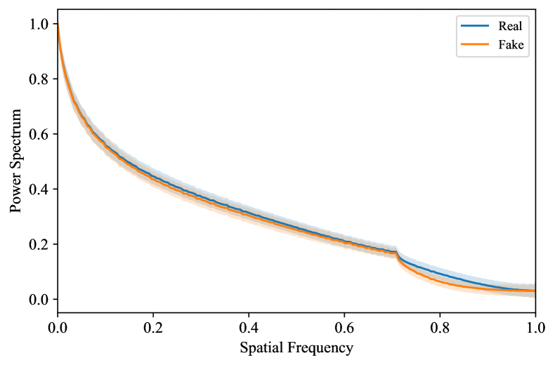
We also observe that high frequency decay discrepancies are not seen in some out-of-the-box GAN models. Specifically, we observe that CRN [6] and IMLE [28] GANs do not have such discrepancies. We show the entire power spectrum for CRN [6] and IMLE [28] GANs in Figure 23 and 24 respectively. Do note that both these models are pre-trained on GTA game data (Another instance of data synthesized from game engines). This further helps to confirm that such discrepancies are not intrinsic.
Supplementary J Dataset Details
For CelebA [29] experiments, we use the officially released train subset consisting of 162, 770 images. For LSUN [43] experiments, we select a random subset of 200, 000 images for training. For StarGAN experiments, we follow the official implementation. For autoencoder experiments, we select a random subset of 1000 images from CelebA-HQ [21].
.
Supplementary K Implementation Details
For GAN experiments, we use Adam optimizer with , and batch size 64. For all CelebA [29] experiments, we used an initial learning rate = . The learning rate was reduced based on FID scores for all experiments. For DCGAN, LSGAN and WGAN-GP experiments, we use the GitHub code used by the Spectral Regularization paper[10] 555https://github.com/LynnHo/DCGAN-LSGAN-WGAN-GP-DRAGAN-Pytorch. For StarGAN [7], we use the official implementation 666https://github.com/yunjey/stargan with default hyper-parameters. For Spectral Regularization [10] experiments, we use the officially released code 777https://github.com/cc-hpc-itwm/UpConv.
For all autoencoder experiments, we use Adam optimizer with and , batch size 128, initial learning rate and learning rate decay scheme that scales the learning rate by 0.9 when reconstruction error plateaus.
For Fourier synthetic detector [12] experiments, we use the officially released matlab code 888https://github.com/tarikdzanic/FourierSpectrumDiscrepancies for feature extraction and use our own script to perform KNN classification. For FID calculation, we used the open-source Pytorch FID implementation 999https://github.com/mseitzer/pytorch-fid.
More details on hyper-parameters and research reproducibility can be found in: https://keshik6.github.io/Fourier-Discrepancies-CNN-Detection/
