Exploring the pulsational properties of two ZZ Ceti stars

Abstract

Context. We continued our ground-based observing project with the season-long observations of ZZ Ceti stars at Konkoly Observatory. Our present targets are the newly discovered PM J22299+3024, and the already known LP 119-10 variables. LP 119-10 was also observed by the TESS (Transiting Exoplanet Survey Satellite) space telescope in 120-second cadence mode.

Aims. Our main aims are to characterise the pulsation properties of the targets, and extract pulsations modes from the data for asteroseismic investigations.

Methods. We performed standard Fourier analysis of the daily, weekly, and the whole data sets, together with test data of different combinations of weekly observations. We then performed asteroseismic fits utilising the observed and the calculated pulsation periods. For the calculations of model grids necessary for the fits, we applied the 2018 version of the White Dwarf Evolution Code.

Results. We derived six possible pulsation modes for PM J22299+3024, and five plus two TESS pulsation frequencies for LP 119-10. Note that further pulsation frequencies may be present in the data sets, but we found their detection ambiguous, so we omitted them from the final frequency list. Our asteroseismic fits of PM J22299+3024 give $11\,400$ K and $0.46\,M_{\sun}$ for the effective temperature and the stellar mass. The temperature is $\approx 800\,$K higher, while the mass of the model star is exactly the same as it was earlier derived by spectroscopy. Our model fits of LP 119-10 put the effective temperature in the range of $11\,800-11\,900\,$K, which is again higher than the spectroscopic $11\,290\,$K value, while our best model solutions give $M_{*}=0.70\,M_{\sun}$ mass for this target, near to the spectroscopic value of $0.65\,M_{\sun}$, likewise in the case of PM J22299+3024. The seismic distances of our best-fitting model stars agree with the Gaia astrometric distances of PM J22299+3024 and LP 119-10 within the errors, validating our model results.

1 Introduction

About 97 per cent of the stars, including our Sun, will finally end their evolution as white dwarfs. Some of the white dwarf stars show low-amplitude, short-period light variations. These can be found at specific parts of the Hertzsprung–Russell diagram, and form three large groups: these are the GW Vir, the V777 Her (DBV), and the ZZ Ceti (DAV) variables. The hottest objects are the GW Vir (pre-)white dwarfs with $\sim$80 000–180 000 K effective temperatures and hydrogen deficient atmospheres, while the DBV and DAV stars are much cooler, with 22 000–32 000 K and 10 500–13 000 K effective temperatures, respectively, and their atmospheres are dominated by neutral helium (DBV) or hydrogen (DAV). For a summary on the characteristic of the different families of white dwarf pulsators, see the review of Córsico et al. (2019).

The most populous group is that of ZZ Ceti, as about 80 per cent of the known pulsating white dwarfs belong to this group. Besides these, new groups of pulsating white dwarf stars have been identified recently, such as the extremely low-mass DA pulsators (ELM-DAVs; Hermes et al. 2012), the extremely low-mass pulsating pre-white dwarf stars (pre-ELM WD variables; Maxted et al. 2013), and the so-called hot DAV stars (Kurtz et al. 2008, 2013; Romero et al. 2020) located at $\sim 30\,000\,$K effective temperatures. Light variations were also detected in DQV variables with atmospheres rich in helium and carbon (Montgomery et al. 2008). However, the observed variability of DQ objects could be explained by effects other than global pulsations, e.g. rapid rotation (Williams et al. 2016). ZZ Ceti variables in detached white dwarf plus main-sequence (MS) binaries have also become known (Pyrzas et al. 2015). For comprehensive reviews on the characteristics of pulsating white dwarf stars, see the papers of Winget & Kepler (2008), Fontaine & Brassard (2008), Althaus et al. (2010), Córsico et al. (2019), and Córsico (2020).

Compact stars, such as white dwarfs, are unique space laboratories. However, the only way we can study their internal structure is by investigating the excited waves propagating thorough their interiors, by means of asteroseismology. This makes the search for new pulsators among white dwarfs an important effort. This is why we have initiated a survey searching for new pulsating white dwarf targets for the TESS (Transiting Exoplanet Survey Satellite) space telescope (Bognár et al. 2018, 2019a). One of our new discoveries was PM J22299+3024, a new pulsator candidate (Bognár et al. 2019a).

Pulsation modes detected in such objects are low horizontal-degree ($\ell=1$ and $2$), low-to-mid radial-order $g$-modes with periods ranging from a couples of minutes to about half an hour, and with amplitudes in the millimagnitude range. The periods of these modes are sensitive to the global stellar structure, the stellar rotation, the inner chemical stratification, and the dynamical processes operating in them, which highlights the great potential of asteroseismological investigations.

We note that different pulsational behaviour is observed at different parts of the ZZ Ceti instability strip. While the hotter objects are more likely to show pulsation frequencies with stable amplitudes and phases, this changes as we investigate objects closer to the red edge (at lower effective temperatures) of the instability domain. At this part, short-term (days–weeks-long) amplitude and phase changes are more common, while we detect longer-period and larger-amplitude pulsations than in the hotter objects. Thanks to the Kepler observations, the so-called outburst events were also exposed in such objects, which means recurring increases in the stellar flux (up to 15 per cent) in cool ZZ Ceti stars (see e.g. Bell et al. 2017a). This phenomenon might be in connection with the cessation of pulsations at the empirical red edge of the ZZ Ceti instability strip (Hermes et al. 2015).

The study of white dwarf stars contributes to the understanding of star formation and evolution, and in addition, by investigating their interiors, we can use them as cosmic laboratories to study the behaviour of material under extreme pressure and temperature conditions, and measure the age of their parent stellar population. We know about 260 ZZ Ceti stars (Córsico 2020) currently, nonetheless, only a limited number of pulsation modes are known for most of them, usually the results of the short discovery runs. This is mainly because of the faintness of these objects, and because of the limited access of ground-based telescopes large enough for follow-up observations. However, we need more pulsation modes for asteroseismology for sufficient constraints on the physical parameters of the stars. Fortunately, there are several ways to collect more information on pulsating white dwarf stars.

International campaigns, such as the Whole Earth Telescope (WET; Nather et al. 1990) proved already that we can extract sufficient number of pulsation frequencies by such observations for performing asteroseismic modelling. Another way is to utilise space-based time-series photometry of white dwarf variables. These space-based observations gave boost to the investigations of such objects. During the nominal Kepler mission and its K2 extension, 81 ZZ Ceti stars were observed, and the analyses of 32 of them have been published so far, see e.g. Hermes et al. (2017a, b); Bell et al. (2017b), and Córsico (2020). Published results have already demonstrated the value of the TESS data, too, focusing on a DBV star (Bell et al. 2019), several ZZ Ceti stars (Bognár et al. 2020; Althaus et al. 2020), and GW Vir variables (Córsico et al. 2021).

We follow a third way, and perform long-term single-site ground-based observations of selected targets not observed extensively before, such as in the case of LP 119-10, presented in this paper. Considering LP 119-10, only the result of the discovery run presenting one period has been published so far. With this publication on PM J22299+3024 and LP 119-10, we continue our efforts to introduce the results of our long-term ground-based observations on pulsating white dwarf stars in a series of papers, see e.g. Bognár et al. (2009), Paparó et al. (2013), Bognár et al. (2014), Bognár et al. (2016), and Bognár et al. (2019b).

2 Observations and data reduction

We performed the observations with the 1-m Ritchey–Chrétien–Coudé telescope located at the Piszkéstető mountain station of Konkoly Observatory, Hungary. We obtained data with an FLI Proline 16803 CCD camera in white light. The exposure times were selected to be 45 s and 30 s in most cases for PM J22299+3024 (fainter target) and LP 119-10, respectively. We applied longer exposures, up to 60 s, in the case of unfavourable weather conditions. The read-out time was $\sim$3 s.

We reduced the raw data frames the standard way utilising iraf tasks: we performed bias, dark and flat corrections before the aperture photometry of field stars. We fitted low-order (second- or third-order) polynomials to the resulting light curves, correcting for long-period instrumental and atmospheric trends. This procedure did not affect the known frequency domain of pulsating ZZ Ceti stars, however, made the detection of any possible long-period light variations, e.g. outburst events, difficult or even impossible. Finally, we converted the observational times of every data point to barycentric Julian dates in barycentric dynamical time (BJD_TDB) using the applet of Eastman et al. (2010).

Tables 1 and 2 show the journals of observations of PM J22299+3024 and LP 119-10, respectively. We collected data on 14 and 6 nights in the 2018 and 2019 observing seasons on PM J22299+3024, respectively, covering 97 and almost 40 hours with our measurements, while we observed LP 119-10 on 15 nights in one season, which resulted in the collection of 86 hours of photometric data on this target.

Table 1: Journal of observations of PM J22299+3024. ‘Exp’ is the integration time used, N is the number of data points, and $\delta T$ is the length of the data sets including gaps. Weekly observations are denoted by ‘a,b,c,d,e,f,g’ letters in parentheses.

Run	UT Date	Start time	Exp.	N	$\delta T$
		(BJD-2 450 000)	(s)		(h)
01(a)	2018 Jul 20	8320.346	30	546	5.64
02(b)	2018 Sep 07	8369.268	30	779	8.77
03(b)	2018 Sep 10	8372.267	45	580	8.51
04(b)	2018 Sep 11	8373.280	45	596	8.41
05(b)	2018 Sep 12	8374.264	45	652	8.81
06(c)	2018 Sep 20	8382.248	45	600	8.35
07(c)	2018 Sep 21	8383.244	45	307	4.19
08(d)	2018 Oct 11	8403.221	45	550	7.49
09(d)	2018 Oct 12	8404.229	45	526	7.34
10(d)	2018 Oct 13	8405.238	45	532	7.12
11(d)	2018 Oct 14	8406.220	45	546	7.57
12(e)	2018 Nov 04	8427.188	40	475	6.37
13(e)	2018 Nov 06	8429.191	40	351	4.24
14(e)	2018 Nov 07	8430.182	40	360	4.49
Total:			7400		97.30
15(f)	2019 Sep 21	8748.258	30	913	8.27
16(f)	2019 Sep 22	8749.260	60	322	6.24
17(g)	2019 Oct 24	8781.213	30	648	5.92
18(g)	2019 Oct 25	8782.217	30	742	6.72
19(g)	2019 Oct 26	8783.213	30	769	7.00
20(g)	2019 Oct 27	8784.215	30	625	5.65
Total:			4019		39.80

Table 2: Journal of observations of LP 119-10. ‘Exp’ is the integration time used, N is the number of data points, and $\delta T$ is the length of the data sets including gaps. Weekly observations are denoted by ‘a,b,c,d,e,f,g’ letters in parentheses.

Run	UT Date	Start time	Exp.	N	$\delta T$
		(BJD-2 450 000)	(s)		(h)
01(a)	2018 Oct 15	8407.388	30	696	6.74
02(b)	2018 Nov 03	8426.406	20	873	5.64
03(b)	2018 Nov 05	8428.377	30	657	7.35
04(b)	2018 Nov 06	8429.375	30	706	6.58
05(b)	2018 Nov 07	8430.374	30	804	7.48
06(c)	2018 Nov 30	8453.267	40	357	4.38
07(c)	2018 Dec 05	8458.250	30	1051	10.34
08(d)	2019 Jan 03	8487.235	30	376	3.68
09(d)	2019 Jan 07	8490.511	60	217	3.87
10(d)	2019 Jan 07	8491.216	30	318	3.03
11(e)	2019 Feb 07	8522.277	30	587	5.61
12(e)	2019 Feb 11	8526.346	30	505	4.72
13(e)	2019 Feb 12	8527.214	30	846	7.71
14(f)	2019 Mar 12	8555.242	30	649	5.87
15(g)	2019 Apr 06	8580.269	30	374	3.47
Total:			9016		86.47

Figures 1 and 2 show the normalised differential light curves of PM J22299+3024, respectively, while the plot of Fig. 3 represents the ground-based light curves of LP 119-10.

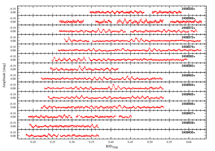
Figure 1: Normalised differential light curves of PM J22299+3024 obtained in the 2018 observing season.

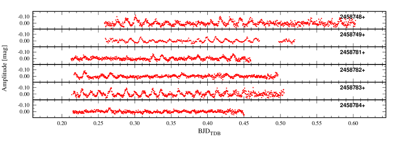
Figure 2: Normalised differential light curves of PM J22299+3024 obtained in the 2019 observing season.

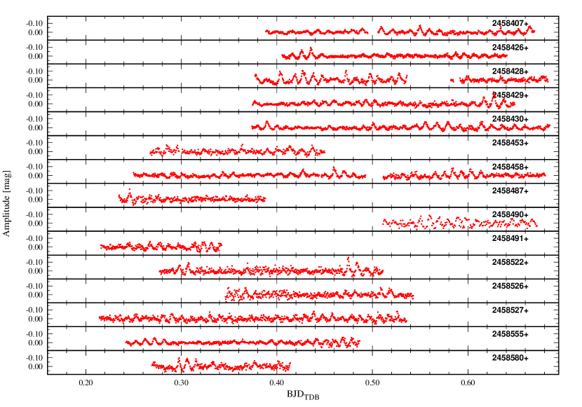
Figure 3: Normalised differential light curves of LP 119-10.

3 Light curve analysis

We performed standard Fourier analysis on the data sets with the photometry modules of the Frequency Analysis and Mode Identification for Asteroseismology (famias) software package (Zima 2008). We accepted a frequency peak as significant if its amplitude reached the five signal-to-noise ratio (S/N), where the noise level was calculated by the average Fourier amplitude in a $\sim 1700\,\mu$Hz radius vicinity ($150\,$d^-1) of the peak in question (see e.g. in Bognár et al. 2019b). That is, we used higher significance level than the usual 4 S/N; we accepted the highest-amplitude peaks as possible pulsational frequencies during the pre-whitening process of these targets showing complex pulsational behaviour, with several closely spaced peaks in their Fourier transforms (FTs).

3.1 PM J22299+3024

PM J22299+3024 ($G=16.21$ mag, $\alpha_{2000}=22^{\mathrm{h}}29^{\mathrm{m}}58^{\mathrm{s}}$, $\delta_{2000}=+30^{\mathrm{d}}24^{\mathrm{m}}10^{\mathrm{s}}$) was found to be a variable candidate by our research group in 2018 July (Bognár et al. 2019a). We performed survey observations to find new bright white dwarf pulsators for the TESS (Ricker et al. 2015) all-sky survey space mission. At that time we considered it a variable candidate as only one night of observations was available on this target. However, the subsequent observations presented in this paper confirmed that PM J22299+3024 is indeed a new, bright ZZ Ceti star, situated close to the red edge of the instability strip according to spectroscopy (Limoges et al. 2015).

First, we performed the Fourier analysis of the daily and weekly data sets, and finally, we analysed the complete 2018 and 2019 data sets, respectively. We also analysed data sets constructed by various combinations of different consecutive weekly data, testing our frequency solutions on data sets with different spectral windows. These six test data sets were consist of the data of weeks (a+b+c), (b+c+d), (c+d+e), (a+b+c+d), (b+c+d+e), and (f+g), cf. Table 1.

Our set of accepted frequencies is based on the analysis of the combined weekly data subsets. These are listed in Table 3. We accepted frequencies as real pulsation components that was found in at least three subsets. We identified six pulsation frequencies in the $\sim 750-960\,\mu$Hz frequency range. We did not find any combination frequencies.

Table 3: The appearance of the accepted pulsation frequencies of PM J22299+3024 in different combined weekly data subsets.

	frequency [$\mu$Hz]
week(a+b+c)	749.3	837.0	855.2	885.0	922.0	959.5
week(b+c+d)	750.4	840.3	–	885.0	922.1	959.4
week(c+d+e)	–	839.2	853.1	884.4	921.0	960.0
week(a+b+c+d)	750.4	839.6	852.6	885.0	922.0	959.8
week(b+c+d+e)	749.3	–	852.6	885.0	922.0	960.5
week(f+g)	–	–	–	883.8	920.1	949.7
average	749.9	839.0	853.4	884.6	921.5	958.2

Note that, besides the frequencies presented in Table 3, further frequencies can also be identified in our data sets. There may be additional frequencies at around $790-800$, $820$, $860$, $900$, and $970\,\mu$Hz. However, the identification of these components and the establishment of their frequency values was ambiguous, therefore, we omitted them from the set of accepted pulsation frequencies listed in Table 3. The ambiguities of the omitted components have possibly two main sources: $1\,$d^-1 aliasing, and short-term amplitude or phase variations. Figure 5 shows that variations in the amplitudes of the pulsation components occurred indeed from one observing week to another.

One of the main goals of the frequency analysis was to provide periods for the asteroseismic models. The set of accepted frequency components is based on the findings presented in Table 3. We refined the frequencies and amplitudes by fitting the complete 2018 data set by the six accepted components. We utilised the obtained periods as input for the asteroseismic modelling described in Sect. 4.2. We present the Fourier amplitude spectrum of the complete 2018 data set in Fig. 4.

Table 4: PM J22299+3024: frequencies, periods and amplitudes of the six accepted pulsation components based on the 2018 observations. The components are listed in decreasing order of amplitude.

	f	P	Ampl.
	[$\mu$Hz]	[s]	[mmag]
$f_{1}$	960.48	1041.14	7.3
$f_{2}$	852.64	1172.83	5.6
$f_{3}$	884.95	1130.00	5.3
$f_{4}$	839.61	1191.03	5.1
$f_{5}$	921.96	1084.65	3.7
$f_{6}$	749.28	1334.61	2.9

Space-based observations would definitely help to verify our Fourier solution and to resolve the frequency ambiguities. PM J22299+3024 was on the list of proposed objects for TESS measurements, and observations were predicted to be performed between 2019 September 11 and October 7 (cycle 2, sector 16) on this object. However, because of the unexpected field shifts of TESS, the telescope did not observe PM J22299+3024. This was one of the reasons why we decided to collect more data on this target from the ground in 2019.

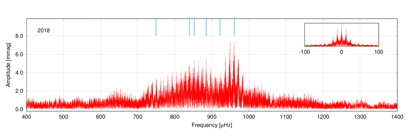
Figure 4: PM J22299+3024: Fourier amplitude spectrum of the complete 2018 data set. We marked the accepted frequencies listed in Table 4 with blue lines. The window function is shown in the inset.

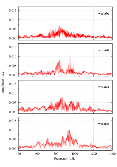
Figure 5: PM J22299+3024: Fourier transform of the weekly data sets with three or more nights of observations.

3.2 LP 119-10

LP 119-10 ($G=15.26$ mag, $\alpha_{2000}=05^{\mathrm{h}}02^{\mathrm{m}}34^{\mathrm{s}}$, $\delta_{2000}=+54^{\mathrm{d}}01^{\mathrm{m}}09^{\mathrm{s}}$) was found to be a variable DA-type white dwarf star by Green et al. (2015). They published one pulsation period for this object at $873.6$ s with an amplitude of $1.27\%$. We observed the star on 15 nights in the 2018/2019 observing season.

Similarly to PM J22299+3024, we performed Fourier analysis not only on the daily, weekly, and the complete data sets, but also on different combinations of the weekly data. We constructed nine such data subsets combining weekly data sets of (a+b+c), (b+c+d), (c+d+e), (d+e+f), (e+f+g), (a+b+c+d), (b+c+d+e), (c+d+e+f), and (d+e+f+g). Table 5 lists the accepted components with peaks close in frequencies in at least four data subsets. As Table 5 shows, we identified five possible pulsation frequencies in the frequency range of $1020-1310\,\mu$Hz. Furthermore, similarly to PM J22299+3024, other possible pulsation frequencies are suspected at around $970-995$, $1040$, $1155$, $1195$, and $1225-1245\,\mu$Hz. Further observations may lead to a more solid identification of these components. We refined the parameter of the five accepted pulsation components by fitting the complete data set. The results are listed in Table 6, while we present the Fourier amplitude spectrum of the complete LP 119-10 data set in Fig. 6.

Table 5: Values of the accepted pulsation frequencies of LP 119-10 derived by the different combined weekly data subsets.

	frequency [$\mu$Hz]
week(a+b+c)	1022.5	1110.3	–	1214.7	1301.9
week(b+c+d)	1022.5	–	1180.5	1215.1	1301.4
week(c+d+e)	–	1110.1	1180.0	–	1305.9
week(d+e+f)	–	–	1180.0	1222.2	1308.5
week(e+f+g)	–	1114.7	1182.2	–	1308.5
week(a+b+c+d)	1022.4	1110.8	–	1214.7	1303.8
week(b+c+d+e)	1022.1	1110.8	1179.7	1218.7	1306.2
week(c+d+e+f)	–	1110.5	1180.1	1219.0	1308.5
week(d+e+f+g)	–	1110.1	1180.0	1222.1	1308.5
average	1022.4	1111.1	1180.4	1218.0	1305.9

Table 6: LP 119-10: list of the set of accepted frequencies based on the whole 2018–2019 data set. The frequencies are listed in decreasing order of amplitude.

	f	P	Ampl.
	[$\mu$Hz]	[s]	[mmag]
$f_{1}$	1218.99	820.35	6.2
$f_{2}$	1179.72	847.66	5.7
$f_{3}$	1022.06	978.42	5.4
$f_{4}$	1302.90	767.52	4.4
$f_{5}$	1110.84	900.22	3.7

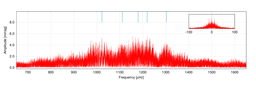
Figure 6: LP 119-10: Fourier amplitude spectrum of the complete data set. We mark the accepted frequencies listed in Table 6 with blue lines. The window function is shown in the inset.

3.2.1 TESS observations

TESS observed LP 119-10 for $24.9$ days in sector 19 with the 120-second short-cadence mode. We downloaded the light curves from the Mikulski Archive for Space Telescopes (MAST), and extracted the PDCSAP fluxes provided by the Pre-search Data Conditioning Pipeline (Jenkins et al. 2016). We omitted the obvious outliers. The resulting light curve consists of 16 494 data points (with a gap), as it can be seen on Fig 7.

The Fourier analysis of the TESS data revealed three significant frequencies above the 4 S/N limit, listed in Table 7. Comparing the frequency contents of the ground-based and space-based observations, we can find one common frequency ($f_{2}=f_{3,TESS}$). The other two frequencies are new detections, including the dominant TESS frequency. This suggests amplitude variations on time scales of months, supported by the different Fourier transforms of the weekly data sets plotted in Fig. 9. Figure 8 shows the Fourier transform of the TESS data set.

Figure 7: TESS light curve of LP 119-10.

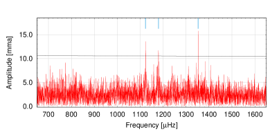
Figure 8: LP 119-10: Fourier transform of the TESS light curve. We marked the frequencies listed in Table 7 with blue lines. The black line denotes the 4 S/N significance level.

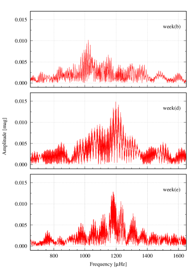
Figure 9: LP 119-10: Fourier transform of the three weekly data sets consist of more than two nightly runs.

Table 7: LP 119-10: set of of frequencies derived by the TESS data set. The frequencies are listed in decreasing order of amplitude.

	f	P	Ampl.
	[$\mu$Hz]	[s]	[mma]
$f_{1,TESS}$	1352.58	739.33	15.8
$f_{2,TESS}$	1123.42	890.14	13.6
$f_{3,TESS}$	1179.79	847.66	11.8

4 Asteroseismology

We built model grids for the asteroseismic investigations of both PM J22299+3024 and LP 119-10, utilising the White Dwarf Evolution Code (wdec) version presented in 2018 (Bischoff-Kim & Montgomery 2018). This updated version of the wdec uses mesa (Modules for Experiments In Stellar Astrophysics; Paxton et al. 2011, version r8118) equation of states and opacity routines.

The starting model is a hot ($\sim 100\,000$ K) polytrope, which is evolved down to the requested temperature. The model we finally obtain is a thermally relaxed solution to the stellar structure equations. The convection is treated within the mixing length theory (Bohm & Cassinelli 1971). We chose to use the $\alpha$ parametrization, according to the results of Tremblay et al. (2015).

We compute the set of possible $\ell=1$ and $2$ eigenmodes for each model according to the adiabatic equations of non-radial stellar oscillations (Unno et al. 1989). The goodness of the fit between the observed ($P_{i}^{\mathrm{obs}}$) and calculated ($P_{i}^{\mathrm{calc}}$) periods is characterised by the root mean square ($\sigma_{\mathrm{{rms}}}$) value calculated for every model with the fitper program of Kim (2007):

$$\sigma_{\mathrm{{rms}}}=\sqrt{\frac{\sum_{i=1}^{N}(P_{i}^{\mathrm{calc}}-P_{i}^{\mathrm{obs}})^{2}}{N}}$$ (1)

where N is the number of observed periods.

4.1 The coarse (master) model grid

At first, we built a coarse (master) model grid, covering a wide parameter space in effective temperature and stellar mass. For this, we varied six input parameters of the wdec: $T_{\mathrm{eff}}$, $M_{*}$, $M_{\mathrm{{env}}}$ (the mass of the envelope, determined by the location of the base of the mixed helium and carbon layer), $M_{\mathrm{H}}$, $X_{\mathrm{{He}}}$ (the helium abundance in the C/He/H region), and $X_{\mathrm{O}}$ (the central oxygen abundance). The second column of Table 8 shows the parameter space we covered with the master grid, and the step sizes applied.

Table 8: The parameter spaces covered by the master grid and the refined grids. The step sizes are in parentheses.

	master grid	refined grid – PM J22299+3024	refined grid – LP 119-10
$T_{\mathrm{eff}}$ [K]	$10\,000-13\,500$ [250]	$11\,000-11\,500$	$11\,500-12\,000$ [100]
$M_{*}$ [$M_{\sun}$]	$0.35-0.80$ [0.5]	$0.40-0.50$	$0.67-0.80$ [0.1]
-log$(M_{\mathrm{{env}}}/M_{*})$	$1.5-1.9$ [0.1]	$1.5-1.9$	$1.5-1.9$ [0.1]
-log$(M_{\mathrm{He}}/M_{*})$	$2$ [fixed]	$2$	$2$ [fixed]
-log$(M_{\mathrm{H}}/M_{*})$	$4-9$ [$1.0$]	$4-9$	$4-9$ [$0.5$]
$X_{\mathrm{{He}}}$	$0.5-0.9$ [0.1]	$0.5-0.9$	$0.5-0.9$ [0.1]
$X_{\mathrm{O}}$	$0.5-0.9$ [0.1]	$0.5-0.9$	$0.5-0.9$ [0.1]

4.2 Results on PM J22299+3024

Investigating the master grid, the best-fitting (lowest $\sigma_{\mathrm{{rms}}}$) model was found to be at $T_{\mathrm{eff}}=11\,250\,$K and $M_{*}=0.45\,M_{\sun}$, assuming, that at least half of the modes are $\ell=1$, taking into account the better visibility of $\ell=1$ modes over $\ell=2$ ones (see e.g. Castanheira & Kepler 2008 and references therein). The effective temperature and mass of PM J22299+3024 derived by optical spectroscopy is $T_{\mathrm{eff}}=10\,630\pm 155$ K and $M_{*}=0.46\pm 0.03\,M_{\sun}$ (log $g=7.72\pm 0.05$), respectively (Limoges et al. 2015). That is, our model solution is hotter than we expect from optical spectroscopy, while they are in very good agreement regarding the stellar mass.

As a next step, we built a refined model grid in effective temperature, stellar mass, and the mass of the hydrogen layer, covering the parameter space in $T_{\mathrm{eff}}$ and $M_{*}$ around the best-fitting model found by the master grid. Table 8 lists the parameter space we investigated by this refined grid (third column), and the corresponding step sizes (fourth column, in parentheses).

According to this refined grid, the best-fitting model has $T_{\mathrm{eff}}=11\,400\,$K and $M_{*}=0.46\,M_{\sun}$. We again assumed at least three $\ell=1$ solutions for the six observed modes. In sum, this model fitting gives $\approx 800\,$K higher effective temperature than it was derived by spectroscopy, but according to the refined grid, the mass of the star found to be exactly the same as the spectroscopic solution.

The left panel of Fig. 10 shows the models of the master grid on the $T_{\mathrm{eff}}-M_{*}$ plane, assuming that at least half of the modes are $\ell=1$. The $\sigma_{\mathrm{{rms}}}$ values of the period fits are colour coded. The fitting results of the refined grid are also shown in Fig. 10 (right panel). We list the physical parameters of the two best-fitting model solutions both utilising the master and the refined grids in the first two rows of Table 9, while Table 10 summarises the observed periods and the calculated periods of the best-fitting model of the refined grid.

Table 9: PM J22299+3024: physical parameters of the best-fitting models.

$T_{\mathrm{eff}}$ [K]	$M_{*}$ [$M_{\sun}$]	-log$M_{\mathrm{{env}}}$	-log$M_{\mathrm{He}}$	-log$M_{\mathrm{H}}$	$X_{\mathrm{{He}}}$	$X_{\mathrm{O}}$	$\sigma_{\mathrm{{rms}}}$ (s)	Comments
11 250	0.45	1.7	2.0	4.0	0.8	0.8	0.94	master grid
11 400	0.46	1.7	2.0	4.0	0.8	0.9	0.67	refined grid
10 200	0.54	1.8	2.0	4.0	0.9	0.8	1.06	closer to spectroscopy
Spectroscopy:
10 630	0.46

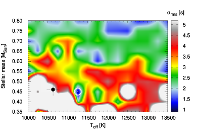
Figure 10: PM J22299+3024: models on the $T_{\mathrm{eff}}-M_{*}$ plane utilising the master grid (left panel) and the refined grid (right panel), assuming that at least half of the modes are $\ell=1$. The $\sigma_{\mathrm{{rms}}}$ values are colour coded. The spectroscopic value is signed with a black dot, while the models with the lowest $\sigma_{\mathrm{{rms}}}$ values are denoted with white open circles.

Table 10: PM J22299+3024: calculated periods of the best-fitting model derived from the refined model grid.

$T_{\mathrm{eff}}$ [K]	$M_{*}$ [$M_{\sun}$]	Periods in seconds ($\ell$)
Model:
11 400	0.46	1041.2 (1)	1083.5 (1)	1172.8 (1)	1335.1 (1)	1129.3 (2)	1192.0 (2)
Observations:
10 630	0.46	1041.1	1084.6	1172.8	1334.6	1130.0	1191.0

4.3 Results on LP 119-10

We have a five- and a seven-period solution for the observations of LP 119-10. Since we fit six grid parameters, we investigated the seven-period solution, including the TESS frequencies.

Applying the master grid and assuming that at least four out of the seven modes are $\ell=1$, the best-fitting model gives $T_{\mathrm{eff}}=11\,750\,$K and $M_{*}=0.75\,M_{\sun}$, with $\sigma_{\mathrm{{rms}}}=1.29\,$s. The spectroscopic values are $T_{\mathrm{eff}}=11\,290\pm 169$ K and $M_{*}=0.65\pm 0.03\,M_{\sun}$ (log $g=8.09\pm 0.05$), respectively (Limoges et al. 2015). That is, we obtain a hotter and higher-mass solution. With further investigations by a refined grid around this solution, the best-fitting model is found to be at $T_{\mathrm{eff}}=11\,900\,$K, $M_{*}=0.70\,M_{\sun}$, with $\sigma_{\mathrm{{rms}}}=0.75\,$s. That is, as in the case of PM J22299+3024, the asteroseismic fittings of LP 119-10 suggest a star hotter than we expect from spectroscopy, but with a stellar mass not far from the spectroscopic value. The first two rows of Table 11 summarise the physical parameters of these best-fitting models, while Table 12 lists the calculated and observed periods of the best-fitting model of the finer grid.

Similarly to PM J22299+3024, we plotted the fitting results both utilising the master and the refined grids in the left and right panels of Fig. 11, respectively.

We also plotted the chemical composition profiles and the corresponding Brunt-Väisälä frequencies for the best-fitting models for both stars in the panels of Fig 12.

Table 11: LP 119-10: physical parameters of the best-fitting models.

$T_{\mathrm{eff}}$ [K]	$M_{*}$ [$M_{\sun}$]	-log$M_{\mathrm{{env}}}$	-log$M_{\mathrm{He}}$	-log$M_{\mathrm{H}}$	$X_{\mathrm{{He}}}$	$X_{\mathrm{O}}$	$\sigma_{\mathrm{{rms}}}$ (s)	Comments
11 750	0.75	1.6	2.0	4.0	0.9	0.5	1.29	master grid
11 900	0.70	1.9	2.0	8.5	0.9	0.5	0.75	refined grid
11 800	0.70	1.9	2.0	8.5	0.5	0.6	1.07	closer to spectroscopy
Spectroscopy:
11 290	0.65

Table 12: LP 119-10: calculated periods of the best-fitting model derived from the refined model grid.

$T_{\mathrm{eff}}$ [K]	$M_{*}$ [$M_{\sun}$]	Periods in seconds ($\ell$)
Model:
11 900	0.70	767.8 (1)	820.0 (1)	890.9 (1)	979.2 (1)	739.4 (2)	849.1 (2)	900.3 (2)
Observations:
11 290	0.65	767.5	820.4	890.1	978.4	739.3	847.6	900.2

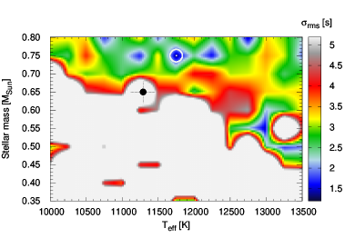
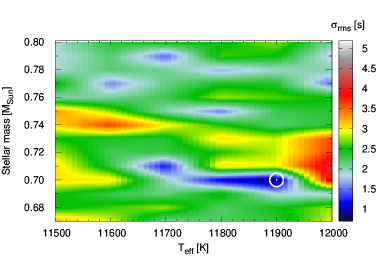
Figure 11: LP 119-10: models on the $T_{\mathrm{eff}}-M_{*}$ plane utilising the master grid (left panel) and the refined grid (right panel), assuming that at least four of the modes are $\ell=1$. The $\sigma_{\mathrm{{rms}}}$ values are colour coded. The spectroscopic value is signed with a black dot, while the models with the lowest $\sigma_{\mathrm{{rms}}}$ values are denoted with white open circles.

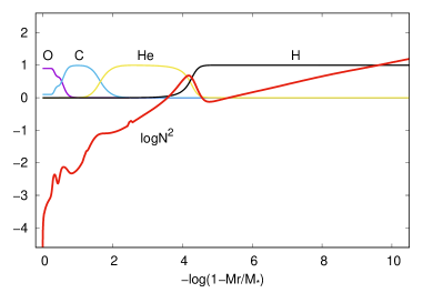
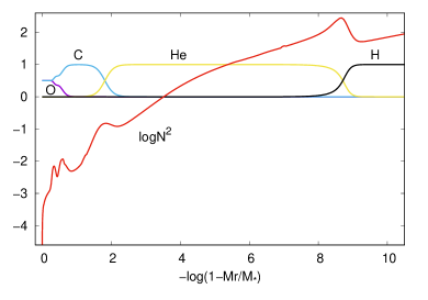
Figure 12: Chemical composition profiles (in fractional abundances), and the corresponding Brunt-Väisälä frequencies ($\mathrm{log}\,N^{2}$) for the best-fitting models in the case of PM J22299+3024 (left panel) and LP 119-10 (right panel), respectively. The model parameters for PM J22299+3024: $T_{\mathrm{eff}}=11\,400\,$K, $M_{*}=0.46\,M_{\sun}$, -log$(M_{\mathrm{{env}}}/M_{*})=1.7$, -log($M_{\mathrm{He}}/M_{*})=2$, -log$(M_{\mathrm{H}}/M_{*})=4$, $X_{\mathrm{{He}}}=0.8$, $X_{\mathrm{O}}=0.9$. The model parameters for LP 119-10: $T_{\mathrm{eff}}=11\,900\,$K, $M_{*}=0.70\,M_{\sun}$, -log$(M_{\mathrm{{env}}}/M_{*})=1.9$, -log($M_{\mathrm{He}}/M_{*})=2$, -log$(M_{\mathrm{H}}/M_{*})=8.5$, $X_{\mathrm{{He}}}=0.9$, $X_{\mathrm{O}}=0.5$.

4.4 Models closer in effective temperature and stellar mass to the spectroscopic solutions

For comparison, we covered the $T_{\mathrm{eff}}$ – $M_{*}$ parameter space in the $\pm 3\sigma$ vicinity of the spectroscopic solutions both for PM J22299+3024 and LP 119-10. That is, this grid for PM J22299+3024 covers the parameter range of $10\,200-11\,100$ K in effective temperature, and $0.37-0.55\,M_{\sun}$ in stellar mass. The step sizes were the same as we used for the refined grids described before. In the case of LP 119-10, we covered the effective temperature and stellar mass parameter ranges of $10\,800-11\,800$ K and $0.56-0.74\,M_{\sun}$, respectively.

In the case of PM J22299+3024, assuming that at least half of the modes are $\ell=1$, the model with the lowest $\sigma_{\mathrm{{rms}}}$ has $T_{\mathrm{eff}}=10\,200$ K, and $M_{*}=0.54\,M_{\sun}$ ($\sigma_{\mathrm{{rms}}}=1.06$ s).

For LP 119-10, the best-fitting model utilising seven modes with at least four $\ell=1$ ones, has $T_{\mathrm{eff}}=11\,800\,$K, and $M_{*}=0.70\,M_{\sun}$ ($\sigma_{\mathrm{{rms}}}=1.07\,$s)

For completeness, we also list the physical parameters of these two model solutions in Tables 9 and 11. We can see that the lowest $\sigma_{\mathrm{{rms}}}$ values belong to the models we found utilising the refined grid but not taking into account the spectroscopic solutions.

4.5 Asteroseismic distances

There is an excellent way to validate our asteroseismic solutions: by comparing the seismic distances calculated by the models with the astrometric distances provided by the Gaia space mission (Gaia Collaboration et al. 2016), see e.g. the example in Bell et al. (2019). In calculating a seismic distance, at first we have to check the luminosity of the model. Knowing the luminosity value $\mathrm{log}\,(L/L_{\sun})$, and the bolometric magnitude of the Sun ($M_{bol,\sun}=4.74$), we can derive the bolometric magnitude of the star using the correlation $M_{bol}=M_{bol,\sun}-2.5\mathrm{log}(L/L_{\sun})$. Now we need the bolometric correction factor (BC) to calculate the absolute visual magnitude of the star: $M_{V}=M_{bol}-\mathrm{BC}$. Bergeron et al. (1995) performed colour-index and magnitude calculations using DA and DB model grids. According to table 1 in Bergeron et al. (1995), $\mathrm{BC}=-0.441$ and $-0.611$ at temperatures $11\,000$ and $12\,000$ K, respectively. From this, we derived the bolometric corrections to the actual temperatures with linear interpolations. Next we need the apparent visual magnitude ($m_{V}$) of the star to apply the distance modulus formula and derive the seismic distance with the given model parameters. Following Bell et al. (2019), we utilised the Fourth US Naval Observatory CCD Astrograph Catalog (Zacharias et al. 2012) to find the apparent visual magnitude of the star. At last, we compared the seismic distance derived this way with the Gaia early third release (Gaia Collaboration et al. 2020, hereafter EDR3) geometric distance value published by Bailer-Jones et al. (2021).

Table 13 summarises the results of the different steps in deriving the seismic distances both for PM J22299+3024 and LP 119-10, respectively. We found for PM J22299+3024, that the $T_{\mathrm{eff}}=11\,400\,$K and $M_{*}=0.46\,M_{\sun}$ model of the refined grid provides a seismic distance equal within the errors with the Gaia astrometric distance, that is, they are in excellent agreement. The seismic distance of the much cooler model with $T_{\mathrm{eff}}$ and $M_{*}$ within the $3\sigma$ vicinity of the spectroscopic values suggests a star about 20 pc closer to us. For LP 119-10, both model solutions provide seismic distances in good agreement with the Gaia distance. Note that they have similar physical parameters, thus in this case, we can conclude that both model solutions are acceptable considering the seismic and astrometric distances.

Table 13: Steps in deriving the seismic distances of the stars. We listed the parameters for two models in the case of both stars: the first models belong to the best-fitting models not considering the spectroscopic solutions, while the second models belong to models found in the $\pm 3\sigma$ vicinity of the spectroscopic $T_{\mathrm{eff}}$ and $M_{*}$ values. We also list the Gaia EDR3 geometric distance values for comparison.

	PM J22299+3024		LP 119-10
$T_{\mathrm{eff}}$ [K]	$11\,400$	$10\,200$	$11\,900$	$11\,800$
$M_{*}$ [$M_{\sun}$]	0.46	0.54	0.70	0.70
$\mathrm{log}L/L_{\sun}$	$-2.453$	$-2.742$	$-2.652$	$-2.667$
$M_{bol}$ [mag]	$10.873$	$11.595$	$11.370$	$11.408$
BC [mag]	$-0.509$	$-0.352$	$-0.594$	$-0.577$
$M_{V}$ [mag]	$11.382$	$11.947$	$11.964$	$11.985$
$m_{V}$ [mag]	$16.161\pm 0.01$		$15.294\pm 0.09$
$d_{seismic}$ [pc]	$90.34\pm 0.42$	$69.62\pm 0.32$	$46.3\pm 1.9$	$45.9\pm 1.9$
$d_{Gaia}$ [pc]	$90.92^{+0.55}_{-0.40}$		$45.97\pm 0.09$

5 Summary and discussion

In this paper, we present the pulsational characteristic of two ZZ Ceti stars; our newly discovered PM J22299+3024, and the already known LP 119-10. Both stars show complex pulsational behaviour, revealed by the Fourier transforms of their data sets with several possible pulsation peaks.

We found that both PM J22299+3024, and LP 119-10 show several pulsational frequencies not known before. With more ground-based observations or measurements from the space, they are good candidates to become pulsators rich in known frequencies, that is, with a dozen or more discovered pulsation modes. Considering the usual amplitude and phase variations observed in these type of stars, our observations represents an important snapshot of the current pulsational behaviour of these targets.

In the case of PM J22299+3024, we accepted six pulsation modes in the $1041-1335\,$s period range, and further Fourier amplitude peaks were identified as possible pulsation frequencies. Similarly, in the case of LP 119-10, five pulsation modes were accepted in the $768-978\,$s period range, but also further modes may be present in the ground-based data set. The TESS space telescope also observed this star, and we were able to complement the set of accepted pulsation modes with two additional ones, while the identifications of a third TESS pulsation component confirmed the ground-based detection of the same mode.

There were two important difficulties when we derived the pulsation frequencies. The first one was the usage of single-site ground-based observations, where the 1 d^-1 aliases appear with relatively large amplitudes in the Fourier transforms. This made the identifications of the pulsation peaks ambiguous, especially because the alias structures of closely situated pulsation peaks overlapped, both for PM J22299+3024 and LP 119-10. Another source of the ambiguities was the amplitude and phase variations of the pulsation modes over time-scales shorter than the duration of the observations. This can lead to the emergence of additional peaks, appearing as extended line widths in the Fourier transforms of the data sets. This effect was clearly demonstrated e.g. in the case of the Kepler observations of ZZ Ceti stars showing pulsation modes longer than $\sim 800\,$s (which is the case both for PM J22299+3024 and LP 119-10), presented by Hermes et al. (2017a).

Beyond the frequency analyses of the data sets on these two stars, we performed asteroseismic investigations of both objects. For PM J22299+3024, our best model solution has an effective temperature and stellar mass of $11\,400\,$K and $0.46\,M_{\sun}$, respectively. The stellar mass is the same as the value provided by spectroscopy, but this model is almost $800\,$K hotter than the spectroscopic solution. However, the seismic distance calculated for our best-fitting model is in excellent agreement with the astrometric distance derived by Gaia observations, supporting our results.

Note that in our asteroseismic analysis we calculated periods of model white dwarfs assuming carbon and oxygen (C/O) core. However, in the case of PM J22299+3024, both its asteroseismic and spectroscopic mass fall just between the mass ranges of the helium-core and C/O-core white dwarfs. The so-called low-mass ($M_{*}\leq 0.45\,M_{\sun}$) white dwarf stars are expected to have helium cores and being results of evolution in binary systems, see e.g. Kepler et al. (2016) and references therein, or the evolutionary calculations focusing on helium-core white dwarfs by Althaus et al. (2013).

The model fits of LP 119-10 give effective temperatures in the range of $11\,800-11\,900\,$K, that is, LP 119-10 is more likely to be around the middle of the ZZ Ceti instability strip, rather than close to the red edge, as was suggested by the spectroscopic observations. Considering its mass, we find solutions with $0.70\,M_{\sun}$, which is near to the $0.65\pm 0.03\,M_{\sun}$ spectroscopic value. Similarly to the case of PM J22299+3024, the seismic and astrometric distances are in good agreement.

We compared the central abundances of carbon and oxygen of our best-fitting models on LP 119-10 with the predictions on these parameters based on stellar evolutionary calculations published by Romero et al. (2012). We utilised their data base, and found a stellar model with physical parameters close to our best-matching solutions: it has $T_{\mathrm{eff}}=11\,814\,$K, $M_{*}=0.705\,M_{\sun}$, $-\mathrm{log}(M_{\mathrm{H}}/M_{*})=8.34$, and central oxygen abundance of $X_{\mathrm{O}}=0.66$. That is, evolutionary predictions prefer higher central oxygen abundance than we obtained for our two best-fitting models. Our best model near the spectroscopic parameters, which gives a core oxygen content of $X_{\mathrm{O}}=0.6$ more in accordance with evolutionary predictions, has only slightly higher $\sigma_{\mathrm{rms}}=1.07$ s compared to the very best-fitting one without spectroscopic restriction, which has a lower core oxygen abundance of $X_{\mathrm{O}}=0.5$ and $\sigma_{\mathrm{rms}}=0.75$ s. We cannot distinguish between the two best models based on their asteroseismic distances, since they agree with one another and with the Gaia distance very well.