$\mathrm{SU}(4)$-Symmetric Quantum Spin-Orbital Liquids on Various Lattices

Abstract

An emergent $\mathrm{SU}(4)$ symmetry discovered in the microscopic model for $d^{1}$ honeycomb materials [M. G. Yamada, M. Oshikawa, and G. Jackeli, Phys. Rev. Lett. 121, 097201 (2018).] has enabled us to tailor exotic $\mathrm{SU}(4)$ models in real materials. In the honeycomb structure, the emergent $\mathrm{SU}(4)$ Heisenberg model would potentially have a quantum spin-orbital liquid ground state due to the multicomponent frustration, and we can expect similar spin-orbital liquids also in three-dimensinal versions of the honeycomb lattice. In such quantum spin-orbital liquids, both the spin and orbital degrees of freedom become fractionalized and entangled together due to the strong frustrated interactions between them. Similarly to spinons in pure quantum spin liquids, quantum spin-orbital liquids can host not only spinon excitations, but also fermionic orbitalon excitations at low temperature.

I Introduction

The material realization of an $\mathrm{SU}(N)$ symmetry with $N>2$ was a long-standing problem. The potential of an emergent $\mathrm{SU}(4)$ symmetry in spin-orbital $d^{1}$ honeycomb materials Yamada et al. (2018); Natori et al. (2018) has stimulated research on various $\mathrm{SU}(4)$ models from two to three dimensions Yamada et al. (2018), including a prediction of a spinon-orbitalon Fermi surface Natori et al. (2018) in the three-dimensional (3D) case. In these $d^{1}$ materials with one electron in a $d$-shell, the low-energy effective spin-orbital model becomes the $\mathrm{SU}(4)$ Heisenberg model, which had been previously very difficult to be realized even in cold atomic systems Cazalilla and Rey (2014). Various quantum spin-orbital liquids (QSOLs) are indeed expected in such $\mathrm{SU}(4)$ models.

The $\mathrm{SU}(4)$ Heisenberg models have attractive advantages from a viewpoint of frustrated magnetism. One of the most intriguing features is that another type of frustration called multicomponent frustration exists even in bipartite lattices Corboz et al. (2012). Triangular geometric frustration is not a necessary condition for $\mathrm{SU}(4)$ spin-orbital liquids and thus we are able to discuss several bipartite lattices Corboz et al. (2012); Natori et al. (2018) in this paper as potential hosts of the spin-orbital liquids. Additionally we will also discuss the broken $\mathrm{SU}(4)$ symmetry on the triangular lattice and its consequences. On nonbipartite lattices, the $d^{1}$ material does not host an $\mathrm{SU}(4)$ symmetry, but still possesses a high symmetry enough to have interesting consequences.

Another important consequence of the emergent $\mathrm{SU}(4)$ symmetry is a correspondence between spin and orbital degrees of freedom. In quantum spin liquids (QSLs), as it was most drastically demonstrated in Kitaev spin liquids, low-energy excitations may be fractionalized into fermions Kitaev (2006). In the spin sector, the (fermionic) spin-1/2 excitation is called spinon in distinction from magnon in the symmetry-broken phase. If there is an $\mathrm{SU}(4)$ symmetry in a system with fractionalized spin excitations, there must be a fractionalized excitation even in the orbital sector. We call this fermionic orbital excitation orbitalon in distinction from orbiton in the Jahn-Teller phase Saitoh et al. (2001). While finding bosonic orbitons was one of the central topics in orbital physics Tokura and Nagaosa (2000), hunting fermionic orbitalons has just begun. The $\mathrm{SU}(4)$ symmetry must be an excellent guiding principle to search for fractionalization in the orbital sector.

We usually write down the $\mathrm{SU}(4)$ Heisenberg model in the form of Eq. (1) in terms of the separate spin operators $\bm{S}_{j}$ and orbital ones $\bm{T}_{j}$.

$$H_{\textrm{eff}}=J\sum_{\langle ij\rangle}\Bigl{(}\bm{S}_{i}\cdot\bm{S}_{j}+\frac{1}{4}\Bigr{)}\Bigl{(}\bm{T}_{i}\cdot\bm{T}_{j}+\frac{1}{4}\Bigr{)},$$ (1)

where $J>0$, $\bm{S}_{j}$, and $\bm{T}_{j}$ are (pseudo)spin-$1/2$ operators defined for each site $j$, and the sum is over nearest-neighbor $ij$-bonds. This is a special high-symmetry point of the Kugel-Khomskii model Kugel and Khomskii (1982). A certain type of frustration involving spin and orbital degrees of freedom exists in this Hamiltonian: If the spin sector forms singlets, the orbital sector forms triplets and vice versa, so even a small number of bonds have a strong frustration denying the singlet formation. The frustration survives even on bipartite lattices, which allows us to regard various lattices as candidate QSOLs.

We note that these highly symmetric $\mathrm{SU}(4)$ models are relevant to materials other than $\alpha$-ZrCl₃ originally proposed in Ref. Yamada et al., 2018. For example, the relevance of an $\mathrm{SU}(4)$ QSOL has been discussed for Ba₃CuSb₂O₉ (BCSO) with a decorated honeycomb lattice structure Zhou et al. (2011); Nakatsuji et al. (2012); Corboz et al. (2012). It turned out, however, that the estimated parameters for BCSO are rather far from the model with an exact $\mathrm{SU}(4)$ symmetry Smerald and Mila (2014). (See Refs. Ohkawa, 1983; Shiina et al., 1997; Wang and Vishwanath, 2009; Kugel et al., 2015 for other proposed realization of $\mathrm{SU}(4)$ symmetry, but they do not lead to QSOL because of their crystal structures.) The relevance of the $\mathrm{SU}(4)$ Heisenberg model has been discussed beyond spin-orbital systems recently. Especially, some of the two-dimensional (2D) systems with moiré superlattices may be described by effective $\mathrm{SU}(4)$ models Xu and Balents (2018); Zhu et al. (2019).

In this paper, we first introduce a notion of an emergent $\mathrm{SU}(4)$ symmetry in spin-orbital systems (Sec. II), derive it in the most general form, and discuss the possibility of various QSOLs in the material realization of the $\mathrm{SU}(4)$ Heisenberg models (Sec. III). Next, we consider the triangular lattice as a representative nonbipartite lattice, discuss its realization, and introduce an exotic frustrated Hamiltonian with an almost $\mathrm{SU}(4)$ symmetry (Sec. IV). Finally, we will summarize this paper and remark some future directions (Sec. V). To describe technical details, five Appendices A-E are given.

II $\mathrm{SU}(4)$ spin-orbital liquids

II.1 Dirac spin-orbital liquid

Before moving on to the material proposal, we would like to review what kind of spin-orbital liquids can be expected in $\mathrm{SU}(4)$ Heisenberg models. The well-established and most famous one is a Dirac spin-orbital liquid in the $\mathrm{SU}(4)$ Heisenberg model on the honeycomb lattice. This state is found by a numerical study Corboz et al. (2012), but is algebraically simple at the same time, so it is informative to explain the analytic property of this ansatz state.

From variational Monte Carlo (VMC) and infinite projected entangled-pair state (iPEPS) calculations, the $\mathrm{SU}(4)$ Heisenberg model on the honeycomb lattice is expected to have a QSOL ground state Corboz et al. (2012). The state is described by a $\pi$-flux Schwinger-Wigner ansatz of complex fermions with an algebraic decay in correlation.

In order to derive the Schwinger-Wigner representation, first we rewrite the Hamiltonian in terms of the $\mathrm{SU}(4)$ operators up to a constant shift as

$$H_{\textrm{eff}}=\frac{J}{4}\sum_{\langle ij\rangle}P_{ij}=\frac{J}{4}\sum_{\langle ij\rangle}\sum_{\alpha\beta}S_{\alpha}^{\beta}(i)S_{\beta}^{\alpha}(j),$$ (2)

where a spin state at each site forms a fundamental representation of $\mathrm{SU}(4)$, and we define $P_{ij}$ as the permutation operator which swaps the states at sites $i$ and $j$. $\mathrm{SU}(4)$ spin operators $S_{\alpha}^{\beta}(j)$ are obeying

$$[S_{\alpha}^{\beta},S_{\alpha^{\prime}}^{\beta^{\prime}}]=\delta_{\beta\alpha^{\prime}}S_{\alpha}^{\beta^{\prime}}-\delta_{\alpha\beta^{\prime}}S_{\alpha^{\prime}}^{\beta}.$$ (3)

Then, $S_{\alpha}^{\beta}(j)$ can be represented by $S_{\alpha}^{\beta}(j)=f_{j\alpha}^{\dagger}f_{j\beta}$ using a complex fermion $f_{j\alpha}$ with $\alpha=1,\dots,4$. This representation with a Gutzwiller projection $\sum_{\alpha}f_{j\alpha}^{\dagger}f_{j\alpha}=1$ will describe the $\mathrm{SU}(4)$ spin correctly.

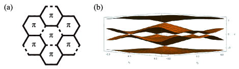
Figure 1: (a) Gauge used in the $\pi$-flux mean-field solution on the honeycomb lattice. For black solid bonds, $\eta_{ij}=1$, while for black dashed bonds $\eta_{ij}=-1$. (b) Dispersion of the $\pi$-flux mean-field solution on the honeycomb lattice.

After inserting this Schwinger-Wigner representation Wen (2002), the mean-field Hamiltonian becomes

$$H_{\textrm{MF}}^{(1)} =-\chi_{0}\sum_{\langle ij\rangle,\,\alpha}\eta_{ij}(f_{i\alpha}^{\dagger}f_{j\alpha}+h.c.),$$ (4)

where $\eta_{ij}=\pm 1$ are determined as shown in Fig. 1(a) and $\chi_{0}$ is some constant. This choice of $\eta_{ij}$ corresponds to a $\pi$ flux through every hexagonal plaquette. Eq. (4) with a Gutzwiller projection gives a variational wavefunction. The dispersion of this $\pi$-flux ansatz is shown in Fig. 1(b). There are two degenerate Dirac cones at $\Gamma$ when it is quarter-filled. Thus, this mean-field solution with a Gutzwiller projection is a candidate Dirac spin-orbital liquid, where complex fermions are coupled to some gauge field, with doubly degenerate Dirac cones. This type of spin-orbital liquids with an algebraic correlation is one typical QSOL expected in the $\mathrm{SU}(4)$ system. This gapless property of the $\mathrm{SU}(4)$ Heisenberg model on the honeycomb lattice is confirmed by various numerical techniques Corboz et al. (2012).

If we use the language of spin-orbital systems, the unbroken $\mathrm{SU}(4)$ symmetry leads to two types of fractionalized excitations, spinons and orbitalons, which are transformed to each other by the $\mathrm{SU}(4)$ rotation. An unbiased density matrix renormalization group (DMRG) study also suggests the existence of a symmetric Mott-insulating state in the large-$U$ limit of the $\mathrm{SU}(4)$ Hubbard model Zhu et al. (2019). We note that this $\pi$-flux ansatz with Dirac cones is analogous to the Affleck-Marston approach Affleck and Marston (1988); Corboz et al. (2012). However, it has recently been claimed that the original $\pi$-flux Dirac spin-orbital liquid might be unstable with respect to the monopole perturbation, leaving the question on the nature of the true ground state still open Calvera and Wang (2021).

II.2 Spinon-orbitalon Fermi surface

Even within the Schwinger-Wigner representation, other phases of spinons and orbitalons are possible depending on lattices and flux sectors. A particularly interesting case is the one with a Fermi surface formed by spinons and orbitalons where the $\mathrm{SU}(4)$ symmetry is not broken. This is a natural generalization of the spinon Fermi surface theory to $\mathrm{SU}(4)$.

While a spinon-orbitalon Fermi surface is not expected on the honeycomb lattice, it was demonstrated that it is a candidate ground state for the hyperhoneycomb lattice Natori et al. (2018), one of the best-known 3D generalizations of the honeycomb lattice Takayama et al. (2015).

In the case of the hyperhoneycomb lattice, the following 0-flux mean-field Hamiltonian is expected to describe the ground state.

$$H_{\textrm{MF}}^{(2)} =-\chi_{0}^{\prime}\sum_{\langle ij\rangle,\,\alpha}(f_{i\alpha}^{\dagger}f_{j\alpha}+h.c.),$$ (5)

where $\chi_{0}^{\prime}$ is some constant. Interestingly, this state has a Fermi surface at quarter filling (one fermion per site), so this mean-field solution describes the spinon-oribitalon Fermi surface as long as the $\mathrm{SU}(4)$ symmetry is not broken. An energetically unfavored $\pi$-flux state also possesses exotic Dirac cones Natori et al. (2018), so the dynamics in the flux sector of the hyperhoneycomb QSOL would also be interesting.

The Affleck-Marston-type flux state Affleck and Marston (1988) may not be stabilized, and may not be a good guess for the ground state away from half filling Lieb (1994). A further study is necessary to reveal the stability of spinon-orbitalon Fermi surfaces more rigorously. We note that a Fermi surface is expected for the $\mathrm{SU}(4)$ Heisenberg model on the triangular lattice Keselman et al. (2020), as well as the critical stripy state Jin et al. (2021).

II.3 Majorana spin-orbital liquids

Another possibility is a Majorana spin-orbital liquid with various (nodal) spectra. Here we would not specify any mean-field solution and its spectrum because we still do not know a lattice hosting such an exotic state. However, the $\mathrm{SO}(6)$ Majorana representation for $\mathrm{SU}(4)$ spins Azaria et al. (1999); Wang and Vishwanath (2009) to describe a Majorana spin-orbital liquid is mathematically fascinating, and thus we would briefly review only the algebraic structure of this representation. This Majorana representation is first proposed for the $\mathrm{SU}(4)$ Heisenberg model on the square lattice Wang and Vishwanath (2009), but later it was found that the true ground state may be a symmetry-broken phase Corboz et al. (2011).

Mathematically there is an accidental isomorphism between Lie algebras $\mathfrak{so}(6)$ and $\mathfrak{su}(4)$. Strictly speaking, an accidental isomorphism can be used only for Lie algbebras, but we abuse terminology like $\mathrm{SO}(6)\cong\mathrm{SU}(4)$, for simplicity. Here, $\cong$ means local isomorphism. Since $\mathrm{SU}(4)\cong\mathrm{SO}(6),$ we can also find an isomorphism between an antisymmetric tensor representation of $\mathrm{SU}(4)$ and a vector representation of $\mathrm{SO}(6).$ Although we will not explicitly demonstrate these isomorphisms, this is the reason why we can construct an $\mathrm{SO}(6)$ Majorana representation.

The representation is similar to Kitaev’s for the $\mathrm{SU}(2)$ spin Kitaev (2006). First, we divide the $\mathrm{SU}(4)$ fundamental representation into spin and orbital degrees of freedom. Then, a spin $\bm{S}_{j}$ and an orbital $\bm{T}_{j}$ can be decomposed into a cross product of two sets of $\mathrm{SO}(3)$ Majorana fermions.

$$S_{j}^{\gamma} =-\frac{i}{4}\varepsilon^{\alpha\beta\gamma}\eta_{j}^{\alpha}\eta_{j}^{\beta},$$ (6)

$$T_{j}^{\gamma} =-\frac{i}{4}\varepsilon^{\alpha\beta\gamma}\theta_{j}^{\alpha}\theta_{j}^{\beta},$$ (7)

where $\varepsilon^{\alpha\beta\gamma}$ is a Levi-Civita symbol, and $\bm{\eta}$ and $\bm{\theta}$ are $\mathrm{SO}(3)$ Majorana fermions with $\{\eta_{i}^{\alpha},\eta_{j}^{\beta}\}=\{\theta_{i}^{\alpha},\theta_{j}^{\beta}\}=2\delta_{ij}\delta^{\alpha\beta},$ and $\{\eta_{i}^{\alpha},\theta_{j}^{\beta}\}=0.$ These 6 Majorana fermions per site provide a natural basis for the $\mathrm{SU}(4)\cong\mathrm{SO}(6)$ symmetry. The Fock space is redundant and has a dimension $(\sqrt{2})^{6}=8$ at each site. Thus, we have to project it onto the 4-dimensional physical subspace in an $\mathrm{SO}(6)$-symmetric way.

The simplest constraint for the projection would be

$$i\eta_{j}^{x}\eta_{j}^{y}\eta_{j}^{z}\theta_{j}^{x}\theta_{j}^{y}\theta_{j}^{z}=1\quad\textrm{for}\,\forall j,$$ (8)

or

$$i\eta_{j}^{x}\eta_{j}^{y}\eta_{j}^{z}\theta_{j}^{x}\theta_{j}^{y}\theta_{j}^{z}=-1\quad\textrm{for}\,\forall j.$$ (9)

Indeed both Eq. (8) and Eq. (9) can simplify the original $\mathrm{SU}(4)$ Hamiltonian and result in the same Majorana Hamiltonian. In either case, all higher order terms in the $\mathrm{SU}(4)$ Heisenberg model can be reduced into quartic terms:

$$H_{\textrm{Majorana}}\propto-\frac{1}{8}\sum_{\langle ij\rangle}\left(i\bm{\eta}_{i}\cdot\bm{\eta}_{j}+i\bm{\theta}_{i}\cdot\bm{\theta}_{j}\right)^{2}.$$ (10)

Thus, at a saddle point we can define a real mean field to solve self-consistent equations: $\chi_{ij}^{R}=\langle i\bm{\eta}_{i}\cdot\bm{\eta}_{j}+i\bm{\theta}_{i}\cdot\bm{\theta}_{j}\rangle,$ and the mean-field Hamiltonian reads

$$H_{\textrm{MF}}^{R}=\sum_{\langle ij\rangle}\left[-\frac{\chi_{ij}^{R}}{4}\left(i\bm{\eta}_{i}\cdot\bm{\eta}_{j}+i\bm{\theta}_{i}\cdot\bm{\theta}_{j}\right)+\frac{(\chi_{ij}^{R})^{2}}{8}\right].$$ (11)

Notice that the mean field $\chi_{ij}^{R}=-\chi_{ji}^{R}$ is always real.

We note that the fermion number is not conserved except for the $Z_{2}$ parity, and usually we make a mean-field ansatz wavefunction by filling a Fermi sea until half filling. The projection onto the physical subspace is similar to that for the Kitaev model Kitaev (2006). In this Majorana spin-orbital liquid, spinons and orbitalons are in fact intertwined due to the projection Eq. (8) or Eq. (9), and thus we shall call them spin-orbitalons.

III Emergent $\mathrm{SU}(4)$ symmetry

III.1 Honeycomb materials

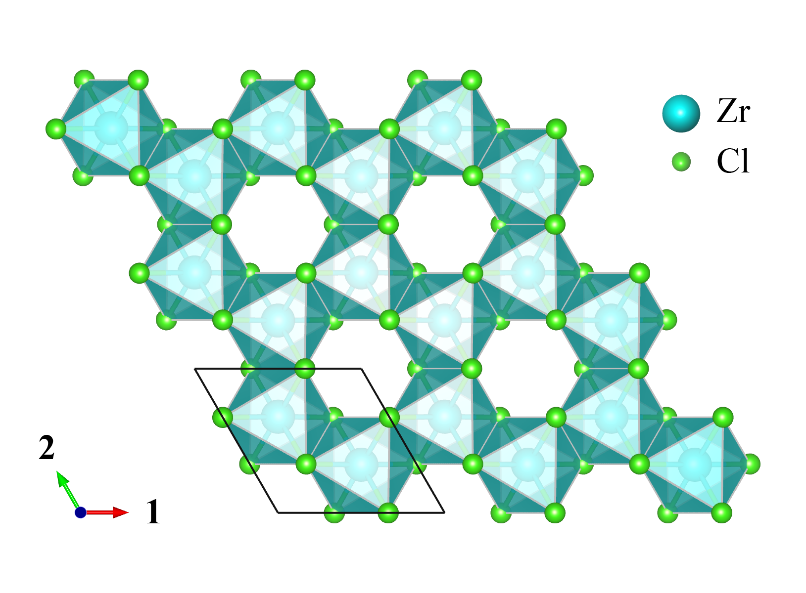
Figure 2: Geometric structure of honeycomb $\alpha$-ZrCl${}_{3}.$ Cyan and light green spheres represent Zr and Cl, respectively. The crystallographic axes are shown and labelled as the 1- and 2-directions. The figure is taken from Ref. Yamada et al., 2018.

From now on we will move on to the material side. In many senses $\alpha$-ZrCl₃ is the first and most important candidate for an emergent $\mathrm{SU}(4)$ symmetry. This material was reported in 1960s by Swaroop and Flengas Swaroop and Flengas (1964a, b). In the reported structure, Zr³⁺ is in the $d^{1}$ electronic configuration, octahedrally surrounded by Cl^-. The crystal structure is supposed to be honeycomb-layered with a high symmetry Swaroop and Flengas (1964a, b) [see Fig. 2]. In the following discussions, we assume that $\alpha$-ZrCl₃ indeed forms well-separated layers of the ideal honeycomb lattice. It should be noted that, however, the crystal structure in Refs. Swaroop and Flengas, 1964a, b may be based on a misaligned powder pattern Daake and Corbett (1978). In addition, a recent density-functional theory calculation suggests that this material might be susceptible to dimerization of the honeycomb layers Ushakov et al. (2020). If the crystal structure is in fact different from the assumed honeycomb one, the theory should also be modified accordingly. Even if the crystal structure is modified, as long as the spin-orbit coupling is unquenched, it probably leads to an exotic orbital magnetism. On the other hand, we can replace atoms as long as the $d^{1}$ electronic configuration is kept. We can think of $\alpha$-$MX_{3}$, with $M=$ Ti, Zr, Hf, etc., $X=$ F, Cl, Br, etc. They are also candidate materials to realize the $\mathrm{SU}(4)$ Heisenberg model on the honeycomb lattice. The case of $\alpha$-TiCl₃ is discussed separately in Appendix A.

The skeletal structure resembles that of $\alpha$-RuCl₃ which is known to be an important candidate for the Kitaev honeycomb model Plumb et al. (2014). We can regard $\alpha$-ZrCl₃ as a particle-hole inversion counterpart of a transition metal halide $\alpha$-RuCl₃ because Ru³⁺ has a $d^{5}$ configuration, while Zr³⁺ has a $d^{1}$ configuration. The ground state is in the $J_{\textrm{eff}}=1/2$ subspace in the former, whereas the ground state is in the $J_{\textrm{eff}}=3/2$ subspace in the latter. We first demonstrate constructing $\mathrm{SU}(4)$ spin models for an effective total angular momentum $J_{\textrm{eff}}=3/2$ on each $M$ of honeycomb $\alpha$-$MX_{3}$, following Ref. Yamada et al., 2018.

The $J_{\textrm{eff}}=3/2$ picture becomes asymptotically exact in the strong SOC limit. This can be achieved by increasing the atomic number of $M$ from Ti to Hf. The compounds $\alpha$-$M$Cl₃ with $M=$ Ti, Zr and related Na₂VO₃ have been already reported experimentally. For simplicity, we only use $\alpha$-ZrCl₃, although exactly the same discussion would apply to $\alpha$-HfCl${}_{3},$ and other honeycomb systems $A_{2}M^{\prime}$O₃ ($A=$ Na, Li, etc., $M^{\prime}=$ Nb, Ta, etc.) as well.

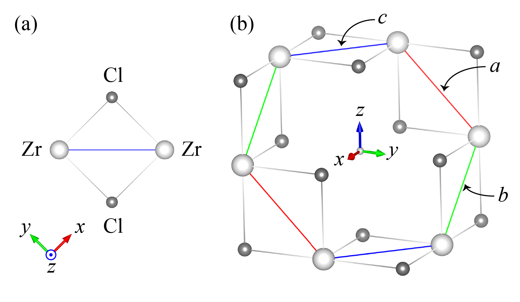
Figure 3: (a) Superexchange pathways between two Zr ions connected by a $c$-bond (blue) in $\alpha$-ZrCl${}_{3}.$ White and grey spheres represent Zr and Cl atoms, respectively. (b) Three different types of bonds in $\alpha$-ZrCl${}_{3}.$ Red, light green, and blue bonds represent $a$-, $b$-, and $c$-bonds on the $yz$-, $zx$-, and $xy$-planes, respectively. The figure is taken from Ref. Yamada et al., 2018.

III.2 Effective Hamiltonian

In the strong-ligand-field limit, the description with one electron in the threefold degenerate $t_{2g}$-shell becomes accurate for $\alpha$-ZrCl₃. The $t_{2g}$-orbitals ($d_{yz}$, $d_{zx}$, and $d_{xy}$-orbitals) are denoted by $a$, $b$, $c$, respectively. Let $a_{j\sigma}$, $b_{j\sigma}$, and $c_{j\sigma}$ represent annihilation operators for these orbitals on the $j$th site of the honeycomb lattice with spin-$\sigma$, and $n_{\xi\sigma j}$ with $\xi\in\{a,b,c\}$ be the corresponding number operators. We also use this $(a,\,b,\,c)=(yz,\,zx,\,xy)$ notation for bonds: each Zr — Zr bond is labeled as $\xi$-bond ($\xi\in\{a,b,c\}$) when the superexchange pathway is on the $\xi$-plane , as depicted in Fig. 3.

Although there are many ways to define a $J_{\textrm{eff}}=3/2$ spinor $\psi$, we here use the following bases: $\psi=(\psi_{\uparrow\uparrow},\psi_{\uparrow\downarrow},\psi_{\downarrow\uparrow},\psi_{\downarrow\downarrow})^{t}=(\psi_{3/2},\psi_{-3/2},\psi_{1/2},\psi_{-1/2})^{t}$, where $\psi_{J^{z}}$ ($J^{z}=\pm 3/2,\,\pm 1/2$) is the annihilation operator for the $\ket{J=3/2,J^{z}}$ state. Assuming the SOC is the largest electronic energy scale, except for the ligand field splitting, fermionic operators can be projected onto the $J_{\textrm{eff}}=3/2$ states by inserting the quartet $\psi_{j\tau\sigma}$ as follows.

$$a_{j\sigma}^{\dagger} \to\frac{\sigma}{\sqrt{6}}(\psi_{j\uparrow\bar{\sigma}}^{\dagger}-\sqrt{3}\psi_{j\downarrow\sigma}^{\dagger}),$$ (12)

$$b_{j\sigma}^{\dagger} \to\frac{i}{\sqrt{6}}(\psi_{j\uparrow\bar{\sigma}}^{\dagger}+\sqrt{3}\psi_{j\downarrow\sigma}^{\dagger}),$$ (13)

$$c_{j\sigma}^{\dagger} \to\sqrt{\frac{2}{3}}\psi_{j\uparrow\sigma}^{\dagger},$$ (14)

where the indices $\tau$ and $\sigma$ of $\psi_{j\tau\sigma}$ represent the pseudoorbital and pseudospin indices, respectively. Here $\bar{\sigma}$ means an opposite spin to $\sigma.$ We begin from the following 6-component Hubbard Hamiltonian for $\alpha$-ZrCl${}_{3}.$

$$H= -t\sum_{\sigma,\langle ij\rangle\in\alpha}(\beta_{i\sigma}^{\dagger}\gamma_{j\sigma}+\gamma_{i\sigma}^{\dagger}\beta_{j\sigma})+h.c.$$

$$+\frac{U}{2}\sum_{j,(\delta,\sigma)\neq(\delta^{\prime},\sigma^{\prime})}n_{\delta\sigma j}n_{\delta^{\prime}\sigma^{\prime}j},$$ (15)

where $t$ is a real hopping parameter through the superexchange pathway shown in Fig. 3(a), $U>0$ is the Hubbard term, $\langle ij\rangle\in\alpha$ means that the bond $\langle ij\rangle$ is an $\alpha$-bond, $\langle\alpha,\beta,\gamma\rangle$ runs over every cyclic permutation of $\langle a,b,c\rangle,$ and $\delta,\delta^{\prime}\in\{a,b,c\}.$ The effects of the Hund coupling $J_{H}$, not included explicitly in Eq. (15), are discussed in Appendix B. Simply by inserting Eqs. (12)-(14), we obtain

$$H=-\frac{t}{\sqrt{3}}\sum_{\langle ij\rangle}\psi_{i}^{\dagger}U_{ij}\psi_{j}+h.c.+\frac{U}{2}\sum_{j}\psi_{j}^{\dagger}\psi_{j}(\psi_{j}^{\dagger}\psi_{j}-1),$$ (16)

where $\psi_{j}$ is the aforementioned $J_{\textrm{eff}}=3/2$ spinor on the $j$th site, and $U_{ij}=U_{ji}$ is a $4\times 4$ unitary matrix

$$U_{ij}=\begin{cases}U^{a}=\tau^{y}\otimes I_{2}&(\langle ij\rangle\in a)\\ U^{b}=-\tau^{x}\otimes\sigma^{z}&(\langle ij\rangle\in b)\\ U^{c}=-\tau^{x}\otimes\sigma^{y}&(\langle ij\rangle\in c)\end{cases},$$ (17)

where $\bm{\tau}$ and $\bm{\sigma}$ are Pauli matrices acting on the $\tau$ and $\sigma$ indices of $\psi_{j\tau\sigma}$, respectively, and $I_{N}$ is an $N\times N$ identity matrix. We note that $U^{a,b,c}$ are Hermitian, so $U_{ji}={U_{ij}}^{\dagger}=U_{ij}$.

Now let us define an $\mathrm{SU}(4)$ gauge transformation,

$$\psi_{j}\to g_{j}\cdot\psi_{j},\qquad U_{ij}\to g_{i}U_{ij}g_{j}^{\dagger},$$ (18)

where $g_{j}$ is an element of $\mathrm{SU}(4)$ chosen for each site $j$. For any loop $C$ on the honeycomb lattice, the $\mathrm{SU}(4)$ flux defined by a product $\prod_{\langle ij\rangle\in C}U_{ij}$ is invariant under the gauge transformation.

For each elementary hexagonal loop (which we call plaquette) $p$ in the honeycomb lattice with the coloring indicated in Fig. 3(b), the product becomes

$$\prod_{\langle ij\rangle\in\hexagon_{p}}U_{ij}=U^{a}U^{b}U^{c}U^{a}U^{b}U^{c}=(U^{a}U^{b}U^{c})^{2}=-I_{4},$$ (19)

corresponding to an Abelian phase $\pi$. Since all the loops in the honeycomb lattice are made of these plaquettes, there exists an $\mathrm{SU}(4)$ gauge transformation which reduces the model (16) to the $\pi$-flux Hubbard model $H$ with a global $\mathrm{SU}(4)$ symmetry.

$$H=-\frac{t}{\sqrt{3}}\sum_{\langle ij\rangle}\eta_{ij}\psi_{i}^{\dagger}\psi_{j}+h.c.+\frac{U}{2}\sum_{j}\psi_{j}^{\dagger}\psi_{j}(\psi_{j}^{\dagger}\psi_{j}-1),$$ (20)

where the definition of $\eta_{ij}=\pm 1$, which is arranged to insert a $\pi$ flux inside each plaquette, is shown in Fig. 1(a).

At quarter filling, i.e. one electron per site, as is the case in $\alpha$-ZrCl₃, the ground state becomes a Mott insulator for a sufficiently large $U/|t|$. In this regime, the effective Hamiltonian for the spin and orbital degrees of freedom, obtained by the second-order perturbation in $t/U$, becomes the Kugel-Khomskii model exactly at the $\mathrm{SU}(4)$ point (1), with $\bm{S}=\bm{\sigma}/2$, $\bm{T}=\bm{\tau}/2$, and $J=8t^{2}/(3U)$ in the basis set after the gauge transformation. We note that the phase factor $\eta_{ij}$ cancels out in this second-order perturbation. This $\mathrm{SU}(4)$ Heisenberg model on the honeycomb lattice is established to host a gapless QSOL Corboz et al. (2012), so we have found a possible realization of a Dirac spin-orbital liquid in $\alpha$-ZrCl₃ with an emergent $\mathrm{SU}(4)$ symmetry.

III.3 Lieb-Schultz-Mattis-Affleck theorem

The nontrivial property of this model may be understood in terms of the Lieb-Schultz-Mattis-Affleck (LSMA) theorem for the $\mathrm{SU}(N)$ spin chains Lieb et al. (1961); Affleck and Lieb (1986); Lajkó et al. (2017); Yao et al. (2019), generalized to higher dimensions Lieb et al. (1961); Affleck (1988); Oshikawa (2000); Hastings (2005); Totsuka . For the honeycomb lattice, which has two sites per unit cell, there is no LSMA constraint for $\mathrm{SU}(2)$ spin systems Jian and Zaletel (2016). Nevertheless, as for the $\mathrm{SU}(4)$ spin system we discuss in this paper, a two-fold ground-state degeneracy is at least necessary to open a gap. This implies the stability of a gapless QSOL phase observed in the $\mathrm{SU}(4)$ Heisenberg model on the honeycomb lattice.

The claim of the LSMA theorem is as follows: Under the unbroken $\mathrm{SU}(N)$ symmetry and translation symmetry, the ground state of the $\mathrm{SU}(N)$ spin system with $n$ fundamental representations per unit cell cannot be unique, if there is a non-vanishing excitation gap and $n/N$ is fractional. This rules out a possibility of a featureless Mott insulator phase, which is defined as a gapped phase with a unique ground state without any spontaneous symmetry breaking or topological order.

The original paper by Affleck and Lieb Affleck and Lieb (1986) only discussed one-dimensional (1D) systems, so we would like to extend this theorem to higher dimensions and systems with a space group symmetry. The proof, based on Oshikawa’s flux insertion argument Oshikawa (2000), is discussed in detail in Appendix D. The proof is not mathematically rigorous but physically intuitive. Here we would just summarize the logic used in the proof.

In the $\mathrm{SU}(2)$ case, the inserted flux is a magnetic flux constructed by $S^{z}$ operators, but in the $\mathrm{SU}(N)$ case we use the following operator instead:

$$I^{0}=\frac{1}{N}\begin{pmatrix}1&0&\cdots&0&0\\ 0&1&&0&0\\ \vdots&&\ddots&&\vdots\\ 0&0&&1&0\\ 0&0&\cdots&0&-(N-1)\end{pmatrix}.$$ (21)

The diagonal elements obey $I^{0}\mod 1=1/N$, so this changes the denominator of the filling fraction from 2 to $N$. This is the intuitive understanding of the theorem, and would be applied to higher dimensions and the case with a space group symmetry.

III.4 Three-dimensional generalizations

Table 1: Tricoordinated lattices discussed in this paper. Space groups are shown in number indices. Nonsymmorphic ones are underlined. $n$ is the number of sites per unit cell.

Lattice name	$\mathrm{SU}(4)$	120° bond	$n$	Space group	LSMA
(10,3)-$a$	✓	✓	4	214	✓
(10,3)-$b$	✓	✓	4	70	✓
(10,3)-$c$	$-$	$-$	6	151	✓
(10,3)-$d$	✓	$-$	8	52	✓
(9,3)-$a$	$-$	$-$	12	166	$-$
$8^{2}.10$-$a$	✓	✓	8	141	$-$
(8,3)-$b$	✓	✓	6	166	✓
stripyhoneycomb	✓	✓	8	66	$-$
(6,3)	✓	✓	2		✓

Generalized 3D honeycomb lattices are sometimes called tricoordinated lattices. Recently, the classification of Kitaev spin liquids on various tricoordinated lattices has been made Hermanns et al. (2015a, b); O’Brien et al. (2016), so we follow their strategy to extend the $\mathrm{SU}(4)$ physics to 3D. We listed all the tricoordinated lattices considered in this paper on Table 1. This table is based on Wells’ classification of tricoordinated lattices Wells (1977). We use a Schläfli symbol $(p,c)$ to label each lattice, where $p$ is the shortest length of the elementary loops of the lattice, and $c=3$ means the tricoordination of each vertex. For instance, (6,3) is the 2D honeycomb lattice, and all the other lattices are 3D lattices, distinguished by an additional letter following Wells Wells (1977). $8^{2}.10$-$a$ is a nonuniform lattice and the notation is different from the other lattices.

By generalizing the discussion of the honeycomb lattice to generic cases, if the $\mathrm{SU}(4)$ orbital flux for any loop $C$ is reduced to an Abelian phase $\zeta_{C}=\pm 1$, i.e. $\prod_{\langle ij\rangle\in C}U_{ij}=\zeta_{C}I_{4}\quad(\textrm{for}\,^{\forall}C)$, the Hubbard model will acquire the $\mathrm{SU}(4)$ symmetry. This relation has been checked for each lattice in Table 1. We note that the flux inside is listed and included in Appendix E.

A checkmark is put on the $\mathrm{SU}(4)$ column if the $\mathrm{SU}(4)$ symmetry exists. Moreover, in order to form a stable structure, the bonds from each site must form a 120-degree structure with an octahedral coordination. This condition has again been checked for each lattice, and indicated on the 120° bond column O’Brien et al. (2016) of Table 1. Finally, we put a checkmark on the LSMA column when the LSMA theorem implies the existence of ground state degeneracy or gapless excitations for the resulting $\mathrm{SU}(4)$ Hubbard model. For example, the LSMA theorem is applicable to the (8,3)-$b$ lattice because $n/N=6/4$ is fractional.

We note that a 3D version of Na₂VO₃ has already been reported Rüdorff et al. (1956). Therefore we can expect synthesis of various 3D polymorphs of ZrCl₃ or $A_{2}M^{\prime}$O₃ with $A=$ Na, Li and $M^{\prime}=$ Nb, Ta, similarly to 3D $\beta$-Li₂IrO₃ Takayama et al. (2015) and $\gamma$-Li₂IrO₃ Modic et al. (2014).

IV Triangular $d^{1}$ system with a broken $\mathrm{SU}(4)$ symmetry

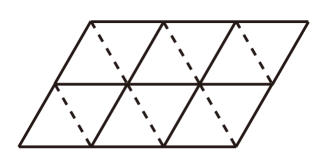
Figure 4: Triangluar $d^{1}$ model. Solid bonds have the $\mathrm{SU}(4)$ Heisenberg interaction, but dashed bonds have an exotic interaction Eq. (24). If we ignore dashed bonds, it becomes the $\mathrm{SU}(4)$ Heisenberg model on the square lattice Corboz et al. (2011).

It would be interesting to investigate $\mathrm{SU}(4)$ Heisenberg models on nontricoordinated lattices. Especially, on the lattice with 1 or 3 sites per unit cell, the LSMA theorem can exclude the possibility of a simply gapped $Z_{2}$ spin liquid and suggests a $Z_{4}$ QSOL or unusual SET phases instead. This can be understood by applying the proof of the LSMA theorem to a cylinder boundary condition because the fourfold ground state degeneracy on a cylinder suggests the existence of a gapless edge mode, or a topological order beyond $Z_{2}$ topological order, for example. The case of the triangular lattice is also mentioned in Ref. Natori et al., 2018.

From now on, we only consider a triangular lattice case for simplicity. Moreover, it may be relevant to some accumulated graphene/transition metal dichalcogenide (TMDC) systems Schrade and Fu (2019). We can easily expect the existence of a $\mathrm{U}(1)$ spin liquid state even for the $\mathrm{SU}(4)$ Heisenberg model on the triangular lattice Keselman et al. (2020). However, unfortunately real triangluar $d^{1}$ systems cannot host an exact $\mathrm{SU}(4)$ Heisenberg model. Instead, as we will show in the following, we find a $\Gamma^{5}$ flux inside each triangluar plaquette and the resulting spin-orbital model becomes exotic, reflecting this additional (non-Abelian) flux.

Similarly to Ba₃IrTi₂O₉ Catuneanu et al. (2015), which is a triangular $d^{5}$ Kitaev material, we can imagine a triangular $d^{1}$ system as a starting point. In this case, each triangular plaquette binds the following flux:

$$\prod_{\langle ij\rangle\in\triangle}U_{ij}=U^{a}U^{b}U^{c}=:i\Gamma^{5}.$$ (22)

For simplicity, we use a chiral representation as follows:

$$\Gamma^{5}=-\tau^{z}\otimes I_{2}=\begin{pmatrix}-I_{2}&0\\ 0&I_{2}\end{pmatrix}.$$ (23)

A gauge transformation can always concentrate a flux matrix to only one bond for each triangular plaquette, so it is enough to focus on one bond $\langle ij\rangle$ with $U_{ij}=i\Gamma^{5}$ in order to derive an effective spin-orbital model by the second-order perturbation in $t/U.$ The rest of the bonds are all $\mathrm{SU}(4)$-symmetric, in which case the discussion is completely parallel to the honeycomb case. As for a bond with $U_{ij}=i\Gamma^{5},$ the second-order perturbation leads to the following spin-orbital model:

$$H_{ij}=J\Bigl{(}\bm{S}_{i}\cdot\bm{S}_{j}+\frac{1}{4}\Bigr{)}\Bigl{(}T_{i}^{z}T_{j}^{z}-T_{i}^{x}T_{j}^{x}-T_{i}^{y}T_{j}^{y}+\frac{1}{4}\Bigr{)},$$ (24)

if $\langle ij\rangle$ is a dashed bond shown in Fig 4. We can expect an exotic frustration, which is different from that in the $\mathrm{SU}(N)$ Heisenberg model. To the best of our knowledge, there is no previous study for this model, so it is worthwhile to study it here.

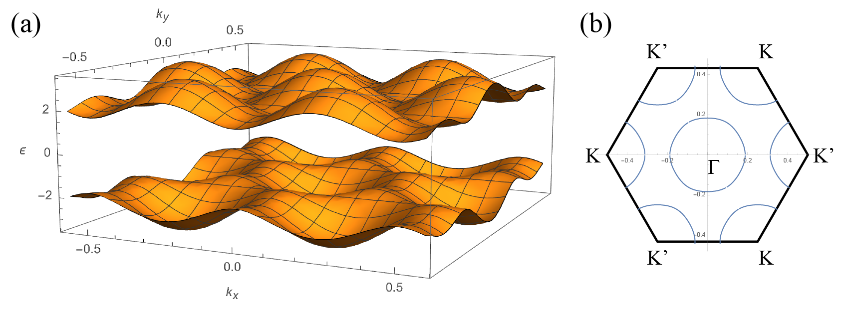
Figure 5: (a) Band structure of the $\Gamma^{5}$-flux state. All bands are doubly degenerate due to the time-reversal and inversion symmetries. (b) Fermi surfaces (blue lines) of the $\Gamma^{5}$-flux state at quarter filling. The Brillouin zone is shown by black lines.

Then, what kind of QSOLs are relevant to this exotic model? One of the most natural possibilities is the $\Gamma^{5}$-flux state. This state is described by the following trial wavefunction $\ket{\Psi_{\textrm{GS}}}$.

$$\ket{\Psi_{\textrm{GS}}}=P_{\textrm{GW}}\ket{\Psi_{\textrm{free}}},$$ (25)

where $\ket{\Psi_{\textrm{free}}}$ is the free-fermionic ground state of the above model with the $\Gamma^{5}$ flux in the case of $U=0$ at quarter filling, and $P_{\textrm{GW}}$ is the Gutzwiller projection onto the space with $N_{j}=1$ for each $j$. The correlation effect of $U\to\infty$ is included in the Gutzwiller projection. Indeed, this state has a spinon-oribitalon Fermi surface. As shown in Fig. 5, two degenerate bands cross the Fermi level at quarter filling and the cross section consists of circular Fermi surfaces.

However, this state most probably suffers from the Bardeen-Cooper-Schrieffer (BCS) instability Hermanns et al. (2015b). The twofold degeneracy of bands and the almost isotropic Fermi surface allow the following BCS ground state instead of the original wavefunction.

$$\ket{\Psi_{\textrm{GS}}^{\prime}} =P_{\textrm{GW}}\ket{\Psi_{\textrm{BCS}}}.$$ (26)

$$\ket{\Psi_{\textrm{BCS}}} =\prod_{\bm{k}}\left(u_{\bm{k}}+v_{\bm{k}}f_{-\bm{k}\downarrow}^{\dagger}f_{\bm{k}\uparrow}^{\dagger}\right)\ket{\Psi_{\textrm{free}}},$$ (27)

where the product about $\bm{k}$ is taken over the Fermi surface, $u_{\bm{k}}$ and $v_{\bm{k}}$ are variational parameters with $u_{\bm{k}}^{2}+v_{\bm{k}}^{2}=1$, and $f_{\bm{k}\sigma}^{\dagger}$ is a creation operator of a spinon/orbitalon with a momentum $\bm{k}$, where $\sigma=\uparrow,\downarrow$ labels the pseudospin index of the Kramers band degeneracy. This describes the standard s-wave pairing of the Cooper pair, while other pairings are also possible.

The energy of the proposed state $\ket{\Psi_{\textrm{GS}}^{\prime}}$ cannot easily be evaluated and probably it requires a VMC simulation about $u_{\bm{k}}$ and $v_{\bm{k}}$. This state describes a kind of gapped spin liquids, while its property is still obscure. Whether or not this state is stabilized is determined from the comparison of energy with other candidate states. The energetic comparison of candidate states based on VMC is left for the future work.

Discussions here are relevant to 1T-TaS₂ Law and Lee (2017); Yu et al. (2017); Murayama et al. (2020) in a symmetric phase without a structural distortion. However, the so-called Star-of-David structure appears after the charge density wave transition, which destroys the orbital degeneracy of the $J_{\textrm{eff}}=3/2$ states. If the symmetric phase survives at very low temperature, 1T-TaS₂ should also be an important playground for the quasi-$\mathrm{SU}(4)$ magnetism.

NaZrO₂ is also a candidate for the same triangular $d^{1}$ state, though the density functional theory (DFT) claims that it is in a nonmagnetic metallic state Assadi and Shigeta (2018). It could possibly lead to the above model after the Mott transition. A DFT study for LiZrO₂ was also found Singh et al. (2004).

V Discussion

In this paper, we made a comprehensive study on various $d^{1}$ spin-orbit coupled systems and discovered that the $\mathrm{SU}(4)$ Heisenberg models appear generically on many tricoordinated bipartite lattices. A part of the results presented in this work were already announced in the previous short communication Yamada et al. (2018). Expanding the original Letter Yamada et al. (2018), in this paper we have presented (i) the proof of the LSMA theorem generalized to higher dimensions, (ii) discussions on the triangular lattice $d^{1}$ system, and (iii) the flux structure of various tricoordinated bipartite lattices.

Even on nonbipartite lattices like the triangular lattice, the $d^{1}$ model is exotic and worth investigating, while they do not host a complete $\mathrm{SU}(4)$ symmetry. The study of actual ground states for those models is left for future work, though we expect QSOLs in general, possibly described by Dirac spin-orbital liquid, spinon-orbitalon Fermi surface liquid, or more exotic Majorana liquids.

The Jahn-Teller term which couples the orbital to the lattice has not been discussed. It typically breaks a symmetry of the lattice, resulting in a Jahn-Teller transition to the low-symmetry phase Tokura and Nagaosa (2000). In order for the symmetric phase to survive, the itinerant quantum fluctuation which can tunnel between classical ground states may be necessary. Thus, the competition between QSOLs and Jahn-Teller phases (orbital order) can be understood in terms of the spinon/orbitalon band width $W\sim J=8t^{2}/(3U)$ Khaliullin and Maekawa (2000). If $J$ is large enough compared to the phonon energy scale to stabilize the (orbital) symmetric state, then the kinetic energy gain of orbitalons may destabilize the Jahn-Teller order. Thus, such energy gain may be maximized around the Mott transition, and thus the 4$d$- or 5$d$-materials with a smaller $U$ may be beneficial.

An indirect sign of a realization of QSOL state in real materials would be the absence of long range order down to the lowest temperatures. Experimentally, muon spin resonance ($\mu$SR) or nuclear magnetic resonance (NMR) experiments can rule out the existence of long-range magnetic ordering or spin freezing in the spin sector. In the orbital sector, a possible experimental signature to observe the absence of orbital ordering or freezing should be electron spin resonance (ESR) Han et al. (2015) or extended X-ray absorption fine structure (EXAFS) Nakatsuji et al. (2012). Especially, (finite-frequency) ESR can observe the dynamical Jahn-Teller effect Nasu and Ishihara (2013, 2015), where the $g$-factor isotropy directly signals the quantum fluctuation between different orbitals Han et al. (2015); Bersuker (1975); Abragam and Bleaney (1970), i.e. the $\mathrm{SU}(2)$ subgroup symmetry in the orbital sector may be evident in the $g$-factor isotropy. This is also applicable to our $t_{2g}$ case because of the shape difference in the $J_{\textrm{eff}}=3/2$ orbitals Romhányi et al. (2017), and the static Jahn-Teller distortion will result in the anisotropy in the in-plane $g$-factors Iwahara et al. (2017). Here we note that the trigonal distortion existing a priori in real materials only splits the degeneracy between the out-of-plane and in-plane $g$-factors, and the splitting of the two in-plane modes clearly indicates some (e.g. tetragonal) distortion.

The emergent $\mathrm{SU}(4)$ symmetry would result in coincidence between the time scales of two different excitations for spins and orbitals observed by NMR and ESR, respectively.

On the other hand, the direct detection of orbitalons may be more challenging. Orbitalons carry an orbital angular momentum. Magnetically an orbital angular momentum is indistinguishable and mixed with a spin by SOC. However, since the orbital fluctuation is coupled to the lattice, an electric field, light, or X-rays can directly affect the orbital sector Tokura and Nagaosa (2000). Especially, a light beam with an orbital angular momentum has been investigated recently Marrucci et al. (2006), and may be useful for the detection of orbitalons. It will be an interesting problem to discover the connection between such technology and fractionalized orbital excitations.

Such orbital physics can be sought in other systems like $f$-electron systems. For example, ErCl₃ may have twofold orbital degeneracy at low temperature Krämer et al. (1999, 2000). In many cases, orbitals have twofold degeneracy at most, so the highest achievable symmetry of QSOLs in spin-orbital materials is $\mathrm{SU}(4).$ Whether it is possible to realize $\mathrm{SU}(6)$ spin systems in spin-orbital systems is an interesting open question. So far a cold atomic system is the only candidate for $\mathrm{SU}(6)$ Nataf et al. (2016). The exploration of hitherto unknown materials with exotic symmetries is still far from being finished, and it is a future problem to make a catalog of these systems.

Appendix A $\alpha$-TiCl₃

As for $\alpha$-TiCl₃, a structural transition and opening of a spin gap at $T=217$ K have been reported Ogawa (1960). This implies a small SOC, as it is consistent with a massively degenerate manifold of spin-singlets expected in the limit of a vanishing SOC Jackeli and Ivanov (2007).

We try to capture the physics of $\alpha$-TiCl₃ by the model without SOC. The model itself was already discussed in Section VIB of Ref. Normand and Oleś, 2008 and Section IIIA of Ref. Chaloupka and Oleś, 2011. This weak-SOC limit is interesting as the valence bond liquid-type states are expected and would potentially explain the observed spin gap behavior.

In addition to the above references, we would like to give an insight from the $\mathrm{SU}(4)$ symmetry. Indeed, the model at $J_{H}=0$ is “locally” $\mathrm{SU}(4)$-symmetric when we flip active orbital on one of the two sites on an isolated bond. Thus, locally the spin-singlet orbital-triplet state, or the spin-triplet orbital-singlet state will lower the energy, potentially leading to the resonating valence bond-like state by covering the honeycomb lattice by $\mathrm{SU}(4)$ dimers.

The above picture is very naive but potentially explains the valence bond formation accompanied by the spin gap transition from the $\mathrm{SU}(4)$ viewpoint. Though there is no global $\mathrm{SU}(4)$ symmetry in the weak-SOC limit, the local $\mathrm{SU}(4)$ symmetry is still useful and is worth mentioning in this Appendix.

Appendix B $\mathrm{SU}(4)$-breaking terms

Of course, real materials do not have a complete $\mathrm{SU}(4)$ symmetry and we have to think of the effect of $\mathrm{SU}(4)$-breaking terms on the spin-orbital liquid states. Especially, we consider the case of $\alpha$-ZrCl₃ and discuss what kind of $\mathrm{SU}(4)$-breaking terms may exist.

The most relevant $\mathrm{SU}(4)$-breaking term would be the Hund coupling $J_{H}$. The Hamiltonian can be written in the simplest form Georges et al. (2013); Yamada et al. (2018) as

$$H= -t\sum_{\sigma,\langle ij\rangle\in\alpha}(\beta_{i\sigma}^{\dagger}\gamma_{j\sigma}+\gamma_{i\sigma}^{\dagger}\beta_{j\sigma})+h.c.+\sum_{j}\left[\frac{U-3J_{H}}{2}N_{j}(N_{j}-1)-2J_{H}\bm{s}_{j}^{2}-\frac{J_{H}}{2}\bm{L}_{j}^{2}+\frac{5}{2}J_{H}N_{j}\right],$$ (28)

where $\alpha$, $\beta$, and $\gamma$ are defined in the same way as Eq. (15), $N_{j}$ is a number operator, $\bm{s}_{j}$ is a total spin, and $\bm{L}_{j}$ is a total effective angular momentum within the $t_{2g}$ manifold. It is easy to see that the perturbation from the original Hamiltonian (Eq. (15)) is small when $J_{H}/U\sim\mathcal{O}(0.1)$, as long as the total $N_{j}$ is conserved.

In addition, it is not difficult to show that in the second-order perturbation the contribution breaking the original $\mathrm{SU}(4)$ symmetry always involves an virtual state with an energy higher than the lowest order by $\lambda$ or $J_{H}.$ Anyway, we can conclude that, as long as we ignore higher order contributions of $J_{H}/U\sim\mathcal{O}(0.1)$, the emergent $\mathrm{SU}(4)$ symmetry would be robust.

We note that recently it was argued that $\mathcal{O}(0.1)$ perturbation of $J_{H}/U$ would not destabilize the $\mathrm{SU}(4)$ spin liquid in the case of BCSO Natori et al. (2019). Although it is not clear this result is applicable to $\alpha$-ZrCl${}_{3},$ we can expect that the stability region of a size $\mathcal{O}(0.1)$ will be reproduced for $\alpha$-ZrCl${}_{3},$ too, by similar mean-field and variational calculations. While this is a preliminary discussion, further studies will disclose the effects of $J_{H}/U$ in the future.

Appendix C Crystalline spin-orbital liquids

Crystalline spin liquids (XSL) Yamada et al. (2017) are defined originally for Kitaev models and the discussion is in Ref. Yamada et al., 2017. We would quickly review the definition and generalize this notion to $\mathrm{SU}(4)$-symmetric models based on the Lieb-Schultz-Mattis-Affleck (LSMA) theorem.

In the context of gapless Kitaev spin liquids as originally proposed in Ref. Yamada et al., 2017, a crystalline spin liquid is defined as a spin liquid state where a gapless point (or a gapped topological phase) is protected not just by the unbroken time-reversal or translation symmetry, but by the space group symmetry of the lattice. This is a simple analogy with a topological crystalline insulator, where a symmetry-protected topological order is protected by some space group symmetry.

Differently from topological crystalline insulators, the classification or identification of crystalline spin liquids is not easy. This is because a symmetry could be implemented projectively in spin liquids and the representation of the symmetry (action) becomes a projective (fractionalized) one. The classification depends not only on its original symmetry of the lattice but also on its PSG, so there are a macroscopic number of possible crystalline spin liquids. The only thing we can do is to identify the mechanism of the symmetry protection for each specific case. In Ref. Yamada et al., 2017, two Kitaev spin liquids are identified, one with three-dimensional (3D) Dirac cones, and the other with a nodal line protected by the lattice symmetry, not by the time-reversal symmetry O’Brien et al. (2016).

Sometimes, however, extended Lieb-Schultz-Mattis-type (LSM-type) theorems can prove the existence of a gapless point or a topological state in the gapped case. Thus, the LSM theorem can potentially prove that some spin liquid is XSL without a microscopic investigation, if we ignore whether it is gapped or gapless Watanabe et al. (2015). This is a subtle point, but LSM-type theorems extended to include a nonsymmorphic symmetry is very powerful to discuss the property of spin liquids abstractly.

Next, we would like to discuss the generalization of the concept of XSL to $\mathrm{SU}(4)$-symmetric models. In the (10,3) lattices listed in Table 1, the unit cell consists of a multiple of 4 sites, and thus the generalized LSMA theorem seems to allow a featureless insulator if we only consider the translation. Following Refs. Parameswaran et al., 2013; Watanabe et al., 2015; Po et al., 2017, however, we can effectively reduce the size of the unit cell by dividing the unit cell by the nonsymmorphic symmetry, and thus the filling constraint becomes tighter with a nonsymmorphic space group. Even in the (10,3) lattices, the gapless QSOL state can be protected by the further extension of the LSMA theorem. We call them crystalline spin-orbital liquids (XSOLs) in the sense that these exotic phases are protected in the presence of both the $\mathrm{SU}(4)$ symmetry and (nonsymmorphic) space group symmetries.

Appendix D Details of the Lieb-Schultz-Mattis-Affleck theorem

The $\mathrm{SU}(N)$ Heisenberg model on the two-dimensional (2D) honeycomb lattice admits the application of the LSMA theorem Lieb et al. (1961); Affleck and Lieb (1986); Oshikawa (2000); Hastings (2005) for $N>2$. However, the original paper by Affleck and Lieb Affleck and Lieb (1986) only discussed one-dimensional (1D) systems, so we would like to extend the claim to higher dimensions and systems with a space group symmetry. Let us first consider a periodic 2D lattice with the primitive lattice vectors $\bm{a}_{1,2}$, as defined in Fig. 2 in the main text. We define the lattice translation operators $\mathcal{T}_{\mu}$ along $\bm{a}_{\mu}$ for $\mu=1,2$.

Here we consider the case with a fundamental representation on each site of the honeycomb lattice, which includes the $\mathrm{SU}(4)$ Heisenberg model discussed in the main text. We call each basis of the $\mathrm{SU}(N)$ fundamental representation flavor. The Hamiltonian of the $\mathrm{SU}(N)$ Heisenberg model on the honeycomb lattice in general can be written as

$$H_{\mathrm{SU}(N)}=\frac{J_{a}}{N}\sum_{\langle ij\rangle\in a}P_{ij}+\frac{J_{b}}{N}\sum_{\langle ij\rangle\in b}P_{ij}+\frac{J_{c}}{N}\sum_{\langle ij\rangle\in c}P_{ij},$$ (29)

up to constant terms, where $J_{\gamma}$s are the bond-dependent coupling constants for the $\gamma$-bonds, as defined in the main text, and $P_{ij}$ is the permutation operator of the flavors between the $i$th and $j$th sites. The translation symmetries, $\mathcal{T}_{1}$ and $\mathcal{T}_{2},$ exist independently of the values of $J_{\gamma}$s, so the following discussions apply to any positive $J_{\gamma}$s. Since the spin-1/2 Heisenberg antiferromagnetic interaction for the $\mathrm{SU}(2)$ spin can also be written as Eq. (29) with $N=2$ dimensional Hilbert space at each site.

Now we discuss the generalization of the LSMA theorem to $\mathrm{SU}(N)$ spin systems Affleck and Lieb (1986); Lajkó et al. (2017); Totsuka in 2 dimensions following the logic of Ref. Oshikawa, 2000. One of the generators $I^{0}$ of the $\mathrm{SU}(N)$ in the fundamental representation is given by the traceless $N\times N$ diagonal matrix:

$$I^{0}=\frac{1}{N}\begin{pmatrix}1&0&\cdots&0&0\\ 0&1&&0&0\\ \vdots&&\ddots&&\vdots\\ 0&0&&1&0\\ 0&0&\cdots&0&-(N-1)\end{pmatrix}.$$ (30)

We introduce an Abelian gauge field $\bm{\mathcal{A}}(\bm{r})$, which couples to the charge $I^{0}$, where $\bm{r}$ is the coordinate.

We assume that the (possibly degenerate) ground states are separated from the continuum of the excited states by a nonvanishing gap, and that the gap does not collapse during the flux insertion process discussed below. We consider the system consisting of $L_{1}\times L_{2}$ unit cells on a torus, namely with periodic boundary conditions $\bm{r}\sim\bm{r}+L_{1}\bm{a}_{1}\sim\bm{r}+L_{2}\bm{a}_{2}$. A ground state, which is $\mathrm{SU}(N)$-symmetric and has a definite crystal momentum (i.e. eigenstate of $\mathcal{T}_{\mu}$ with $\mu=1,\,2$), is chosen as the initial state. We adiabatically increase the gauge field from $\bm{\mathcal{A}}=0$ to $\bm{\mathcal{A}}=\bm{k}_{1}/L_{1}$, so that the “magnetic flux” contained in the “hole” of the torus increases. When the “magnetic flux” reaches the unit flux quantum $2\pi,$ the Hamiltonian of the system becomes equivalent to the initial one. This happens precisely when the Hamiltonian is obtained from the original Hamiltonian with a large gauge transformation. The minimal large gauge transformation with respect to the charge $I^{0}$ is given by

$$\mathcal{U}_{1}=\exp{\left[\frac{i}{L_{1}}\sum_{\bm{r}}\bm{k}_{1}\cdot\bm{r}I^{0}(\bm{r})\right]},$$ (31)

where $\bm{k}_{\mu}$s are primitive reciprocal lattice vectors satisfying

$$\bm{k}_{\mu}\cdot\bm{a}_{\nu}=2\pi\delta_{\mu\nu}.$$ (32)

The large gauge transformation satisfies the commutation relation,

$$\mathcal{U}_{1}\mathcal{T}_{1}=\mathcal{T}_{1}\mathcal{U}_{1}\exp{\left[\frac{2\pi i}{L_{1}}\Bigl{(}I^{0}_{T}-\sum_{\bm{r}\cdot\bm{k}_{1}=2\pi(L_{1}-1)}L_{1}I^{0}\left(\bm{r}\right)\Bigr{)}\right]}.$$ (33)

Here $I^{0}_{T}=\sum_{\bm{r}}I^{0}(\bm{r})$. Since the ground state is assumed to be an $\mathrm{SU}(N)$-singlet when the number of sites is a multiple of $N,$ it belongs to the eigenstate with $I^{0}_{T}=0.$ Furthermore, because eigenvalues of $I^{0}(\bm{r})$ are equivalent to $1/N\mod{1},$ we find,

$${\mathcal{T}_{1}}^{-1}\mathcal{U}_{1}\mathcal{T}_{1}\sim\mathcal{U}_{1}e^{-(2\pi inL_{2}/N)},$$ (34)

where $n$ is the number of sites in the unit cell.

Since the uniform increase in the vector potential does not change the crystal momentum, this phase factor due to the large gauge transformation alone gives the change of the crystal momentum in the flux insertion process. Choosing $L_{2}$ to be coprime with $N,$ we find a nontrivial phase factor when $n/N$ is not an integer. This implies that, if $n$ is not an integer multiple of $N$, the system must be gapless or has degenerate ground states.

For the honeycomb lattice, $n=2,$ and there is no LSMA constraint for $\mathrm{SU}(2)$ spin systems. In contrast, for the $\mathrm{SU}(4)$ spin system we discussed in the main text, the ground-state degeneracy (or gapless excitations) is required even on the honeycomb lattice. Thus, the resulting quantum spin-orbital liquid (QSOL) Corboz et al. (2012) cannot be a “trivial” featureless Mott insulator when the symmetry is not broken spontaneously.

As explained in the above proof, the existence of a nontrivial generator $I^{0}$ is important for this theorem. In the case of $\alpha$-ZrCl₃ discussed in the main text, this element is not included in the generators of the original $\mathrm{SU}(2)\times\mathrm{SU}(2)$ symmetry of the spin-orbital space, but included in the emergent $\mathrm{SU}(4)$ symmetry in the strong spin-orbit coupling limit. Thus, we can say that the $\mathrm{SU}(4)$ symmetry actually protects the nontrivial ground state of the $\mathrm{SU}(4)$ Heisenberg model on the honeycomb lattice.

This proof of the LSMA theorem is not restricted to bosonic systems, and applies to both bosonic and fermionic systems. Thus, the generalization to the (zero-flux) $\mathrm{SU}(N)$-symmetric Hubbard models is straightforward. With $N$-flavor fermionic degrees of freedom in the $\mathrm{SU}(N)$ fundamental representation at each site, the necessary condition for the existence of a featureless insulator is that there exists a multiple of $N$ fundamental representations per unit cell, which can form an $\mathrm{SU}(N)$ singlet. We note that the LSMA theorem for $\mathrm{SU}(N)$ spin systems can be derived from the $U\to\infty$ limit of the $\mathrm{SU}(N)$ Hubbard model at $1/N$ filling. One can also extend the LSMA theorem to the systems with general representations on each site, starting from a Hubbard model. That is, we include an appropriate onsite “Hund” coupling $J_{H}$ in the Hubbard model so that the desired representation have the lowest energy, and then take the $J_{H}\to\infty$ limit afterwards.

The generalization to the 3D case with three translation operators, $\mathcal{T}_{1},$ $\mathcal{T}_{2},$ and $\mathcal{T}_{3},$ is again straightforward and we will omit the proof here, but it is useful to extend the LSMA theorem to the case with a space group symmetry. Recently, tighter constraints are obtained for nonsymmorphic space group symmetries Parameswaran et al. (2013); Watanabe et al. (2015) than what is implied by the LSMA theorem based on the translation symmetries only. This is because a nonsymmorphic symmetry behaves as a “half” translation, which would reduce the size of the effective unit cell.

As a demonstration, here we only discuss the constraint given by one nonsymmorphic (glide mirror or screw rotation) operation $\mathcal{G}$, by generalizing the flux insertion argument as in Ref. Parameswaran et al., 2013. We note that a tighter condition can be derived by dividing the torus into the largest flat manifold, which is called Bieberbach manifold, for some of the nonsymmorphic space groups Watanabe et al. (2015).

Among the 157 nonsymmorphic space groups, the 155 except for $I2_{1}2_{1}2_{1}$ (No. 24) and $I2_{1}3$ (No. 199) include an unremovable (essential) glide mirror or screw rotation symmetry $\mathcal{G}$ König and Mermin (1999), so we will concentrate on these 155 to show how $\mathcal{G}$ works to impose a stronger constraint on filling. The nonsymmorphic operation $\mathcal{G}$ consists of a point-group operation $G$ followed by a fractional (nonlattice) translation with a vector $\bm{\alpha}$ in a direction left invariant by $G,$ i.e. $\mathcal{G}:\bm{r}\mapsto G\bm{r}+\bm{\alpha}$ with $G\bm{\alpha}=\bm{\alpha}.$ We again assume that the (possibly degenerate) ground states are separated from the continuum of the excited states by a nonvanishing gap, and that the gap does not collapse during the flux insertion process discussed below. A ground state $\ket{\psi},$ which is $\mathrm{SU}(N)$-symmetric and has a definite eigenvalue of all the crystalline symmetries including $\mathcal{G}$ (i.e. eigenstate of $\mathcal{G}$), is chosen as the initial state.

We note that, for every nonsymmorphic space group except for $I2_{1}2_{1}2_{1}$ (No. 24) and its key nonsymmorphic operation $\mathcal{G},$ we can take an appropriate choice of primitive lattice vectors $\bm{a}_{1},$ $\bm{a}_{2},$ $\bm{a}_{3}$ with the following properties Watanabe et al. (2015): (i) The associated translation $\bm{\alpha}$ is along the direction of $\bm{a}_{1}$, and (ii) The plane spanned by $\bm{a}_{2}$ and $\bm{a}_{3}$ is invariant under $G.$ Assuming this condition, we can show the tightest condition derived from only one nonsymmorphic operation $\mathcal{G}.$ For simplicity, we consider the system consisting of $L_{1}\times L_{2}\times L_{3}$ unit cells on a 3D torus (i.e. impose the periodic boundary conditions $\bm{r}\sim\bm{r}+L_{\mu}\bm{a}_{\mu}$ for $\mu=1,2,3$).

We take the smallest reciprocal lattice vector $\tilde{\bm{k}}_{1}$ left invariant by $G,$ i.e. $G\tilde{\bm{k}}_{1}=\tilde{\bm{k}}_{1}$ and $\tilde{\bm{k}}_{1}$ generates the invariant sublattice of the reciprocal lattice along $\tilde{\bm{k}}_{1}.$ We insert a flux on a torus by introducing a vector potential $\bm{\mathcal{A}}=\tilde{\bm{k}}_{1}/L_{1}.$ Since the “magnetic flux” reaches a multiple of $2\pi$ after this process because $\tilde{\bm{k}}_{1}$ is a reciprocal lattice vector, the Hamiltonian of the system becomes equivalent to the initial one. This happens precisely when the Hamiltonian is obtained from the original Hamiltonian with a large gauge transformation. The large gauge transformation to remove the inserted flux is

$$\mathcal{U}_{\tilde{\bm{k}}_{1}}=\exp{\left[\frac{i}{L_{1}}\sum_{\bm{r}}\tilde{\bm{k}}_{1}\cdot\bm{r}I^{0}(\bm{r})\right]}.$$ (35)

Since $\bm{\mathcal{A}}$ is left invariant under $\mathcal{G},$ the inserted flux does not change the eigenvalues of $\mathcal{G}.$ Thus, this phase factor due to the large gauge transformation alone gives the change of the eigenvalue of $\mathcal{G}$ for $\ket{\psi}$ in the flux insertion process. On the other hand,

$${\mathcal{G}}^{-1}\mathcal{U}_{\tilde{\bm{k}}_{1}}\mathcal{G}\sim\mathcal{U}_{\tilde{\bm{k}}_{1}}e^{-(2\pi i\Phi_{G}(\tilde{\bm{k}}_{1})nL_{2}L_{3}/N)},$$ (36)

where $\Phi_{G}(\tilde{\bm{k}}_{1})=\bm{\alpha}\cdot\tilde{\bm{k}}_{1}/(2\pi).$ For an unremovable glide or screw symmetry, this phase factor has to be fractional. Thus, if we write $\Phi_{G}(\tilde{\bm{k}}_{1})=p/\mathcal{S}_{G}$ with $p,\mathcal{S}_{G}$ relatively coprime, we can show a tighter bound for the filling constraint to get a featureless Mott insulator without ground state degeneracy because $\mathcal{S}_{G}>1.$ In fact, to get a featureless Mott insulator $pnL_{2}L_{3}/(N\mathcal{S}_{G})$ must at least be integer. However, if we choose $L_{2}$ and $L_{3}$ relatively prime to $N\mathcal{S}_{G},$ $n$ has to be a multiple of $N\mathcal{S}_{G}.$

If $n$ is not a multiple of $N\mathcal{S}_{G}$ for some nonsymmorphic operation $\mathcal{G},$ this means the existence of degenerate ground states with a different eigenvalue of $\mathcal{G},$ i.e. implies the existence of gapless excitations or a gapped topological order if the symmetry $\mathcal{G}$ is not broken. For example, in the case of the $\mathrm{SU}(4)$ Heisenberg model on the hyperhoneycomb lattice, $n=4,$ and the system can be trivial with respect to the translation symmetry. However, the space group of the hyperhoneycomb lattice includes some nonsymmorphic operations, such as one glide mirror with $\mathcal{S}_{G}=2.$ If we assume that nonsymmorphic symmetries are unbroken, the resulting QSOL (a possible symmetric ground state) cannot be a trivial featureless Mott insulator. Thus, we can say this QSOL is protected by the nonsymmorphic space group symmetry of the lattice and it can be called XSOL.

We note that as for the lattice (10,3)-$d,$ it is not enough to consider only one symmetry operation and one has to consider the interplay of multiple nonsymmorphic operations Parameswaran et al. (2013). The derivation of the tightest bound for all the 157 nonsymmorphic space groups with an $\mathrm{SU}(N)$ symmetry is outside of the scope of this paper. A nonsymmorphic symmetry sometimes exchanges the bond label, and then it only exists when $J_{\gamma}$ obeys some condition. In this limited case, the generalized LSMA theorem only applies in some parameter region defined by this condition.

Appendix E Examples of tricoordinated lattices

The flux configurations for the 3D tricoordinated lattices listed in Table 1 can be treated similarly to the Kitaev models on tricoordinated lattices Kitaev (2006); O’Brien et al. (2016) except for the difference in the gauge group. Following Kitaev Kitaev (2006), we use terminology of the lattice gauge theory. The link variables $U_{ij}$ are Hermitian and unitary (in this case) $4\times 4$ matrices defined for each bond (link) $\langle ij\rangle$ of the lattice. Each link variable depends on its type (color) of the bond as

$$U_{ij}=\begin{cases}U^{a}=\tau^{y}\otimes I_{2}&(\langle ij\rangle\in a)\\ U^{b}=-\tau^{x}\otimes\sigma^{z}&(\langle ij\rangle\in b)\\ U^{c}=-\tau^{x}\otimes\sigma^{y}&(\langle ij\rangle\in c)\end{cases},$$ (37)

where $\bm{\tau}$ and $\bm{\sigma}$ are independent Pauli matrices, following the original gauge (basis) used in Sec. III.2 (not the one used in the previous section). The bond type $abc$ is determined from which plane this bond belongs to in the same way as $\alpha$-ZrCl${}_{3}.$ We note that in the 3D case we actually have six types of bonds with additional $\pm 1$ factors, so $U_{ij}=\pm U^{a},\,\pm U^{b},\,\pm U^{c}$ depending on a detailed structure of the bond $\langle ij\rangle.$ This comes from the spatial dependence of the sign of the wavefunctions of the $d$-orbitals. These additional $\pm 1$ factors can simply be gauged out as described in Ref. Yamada et al., 2018.

In order to find a gauge transformation to get an $\mathrm{SU}(4)$ Hubbard model, we have to check that every Wilson loop operator is Abelian. In an abuse of language, each Wilson loop will be called flux inside the loop. We regard a Wilson loop operator $I_{4}$ as a zero flux, and $-I_{4}$ as a $\pi$ flux. In order to get a desired gauge transformation, it is enough to show that the flux inside every elementary loop $C$ is Abelian:

$$\prod_{\langle ij\rangle\in C}U_{ij}=\zeta_{C}I_{4},$$ (38)

with some phase factors $|\zeta_{C}|=1.$

Since $U_{ij}^{2}=I_{4},$ not all the fluxes are independent. In the case of a $Z_{2}$ gauge field, the constraints between multiple fluxes are called volume constraints O’Brien et al. (2016). However, due to the non-Abelian nature of the flux structure, it is subtle whether they apply. Fortunately, the above $U^{\alpha}$ ($\alpha=a,\,b,\,c$) obeys the following anticommutation relations.

$$\{U^{\alpha},U^{\beta}\}=2\delta^{\alpha\beta}I_{4}.$$ (39)

This algebraic relation proves the product of the fluxes of the loops surrounding some volume must vanish (volume constraints). Moreover, we can easily show that, if every bond color is used even times in each loop, which is a natural consequence for the lattices admitting materials realization, the flux inside should always be Abelian with $\zeta_{C}=\pm 1.$ Actually, every lattice included in Table 2 obeys this condition, so we have already proven all of them have an Abelian flux value.

The remaining subtle problem is which flux these elementary loops have, a zero flux, or a $\pi$ flux. To check this, we need to investigate every loop one by one. To calculate every flux value systematically, we often use space group symmetries to relate two elementary loops, even though the system is in the strong spin-orbit coupling limit. We note that the threefold rotation symmetry of the $xyz$-axes of the Cartesian coordinate is not clear in the original gauge in Sec. III.2. This symmetry is important for some 3D models, although the spin quantization axis along the (111) direction will make this symmetry explicit. We have checked all the elementary loops in the tricoordinated lattices listed here. In most cases, elementary loops of the same length have the same flux due to some symmetry. Only the flux value for the shortest elementary loops is shown in Table 2.

Table 2: Flux value of tricoordinated lattices. Only the flux value for the shortest elementary loops is shown here. Nonsymmorphic space group numbers are underlined. NS means that nonsymmorphic symmetries of the lattice are enough to protect a quantum spin-orbital liquid state. In addition to the contents of Table 1, we also include O’Keeffe’s three-letter codes Delgado Friedrichs et al. (2003a, b).

Wells’	Lattice	O’Keeffe’s	Minimal	Flux
notation	name	code	loop length	value
(10,3)-$a$	hyperoctagon	srs	10	0-flux
(10,3)-$b$	hyperhoneycomb	ths	10	0-flux
(10,3)-$d$		utp	10	0-flux
nonuniform	$8^{2}.10$-$a$	lig	8	$\pi$-flux
(8,3)-$b$	hyperhexagon	etb	8	$\pi$-flux
nonuniform	stripyhoneycomb	clh	6	$\pi$-flux
(6,3)	2D honeycomb	hcb	6	$\pi$-flux

E.1 (10,3)-$a$

First of all, nonsymmorphic symmetries are useful to determine the flux value because nonsymmorphic transformations often do not change the bond coloring and effectively reduce the number of elementary loops. As a concrete example, we take the hyperoctagon lattice (10,3)-$a$ to show its usefulness. (10,3)-$a$ has six elementary loops of length 10 Hermanns and Trebst (2014), and 4 of them are related by the fourfold screw rotation symmetry [see Fig. 6(a)-(d)]. This fourfold screw exchanges the $b$-bonds for the $c$-bonds, but this will not affect the flux value if the flux is Abelian because the choice of the $xyz$-axes and its chirality is arbitrary. The rest two elementary loops [see Fig. 6(e)-(f)] accidentally have the same coloring as they are related by the screw symmetry. Therefore, it is enough to check only two elementary loops, (a) and (e).

$$U^{c}U^{a}U^{c}U^{a}U^{b}U^{a}U^{c}U^{a}U^{c}U^{b} =I_{4},$$ (40)

$$U^{b}U^{a}U^{b}U^{a}U^{c}U^{a}U^{b}U^{a}U^{b}U^{c} =I_{4}.$$ (41)

From the above symmetry arguments, or from volume constraints, we can conclude that all the six elementary loops (of length 10) in (10,3)-$a$ have a zero flux. This result agrees with the fact that this zero-flux configuration is the unique $Z_{2}$ flux configuration that obeys all the lattice symmetries of (10,3)-$a$ O’Brien et al. (2016).

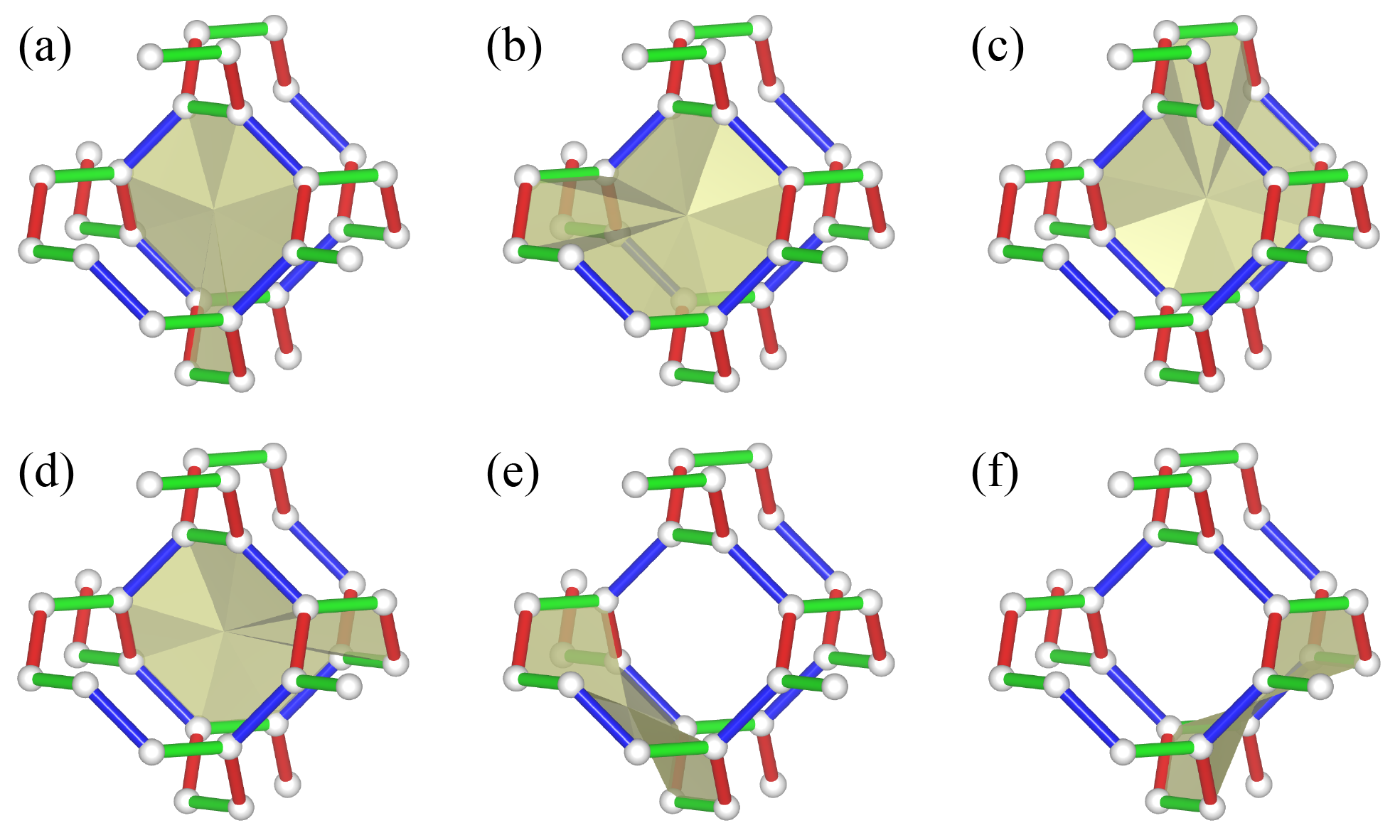
Figure 6: Part of (10,3)-$a.$ All the six elementary loops Hermanns and Trebst (2014) are highlighted by yellow surfaces. Loops (a)-(d) are related by the fourfold screw rotation, and loops (e) and (f) are again related by the same symmetry.

E.2 (10,3)-$b$

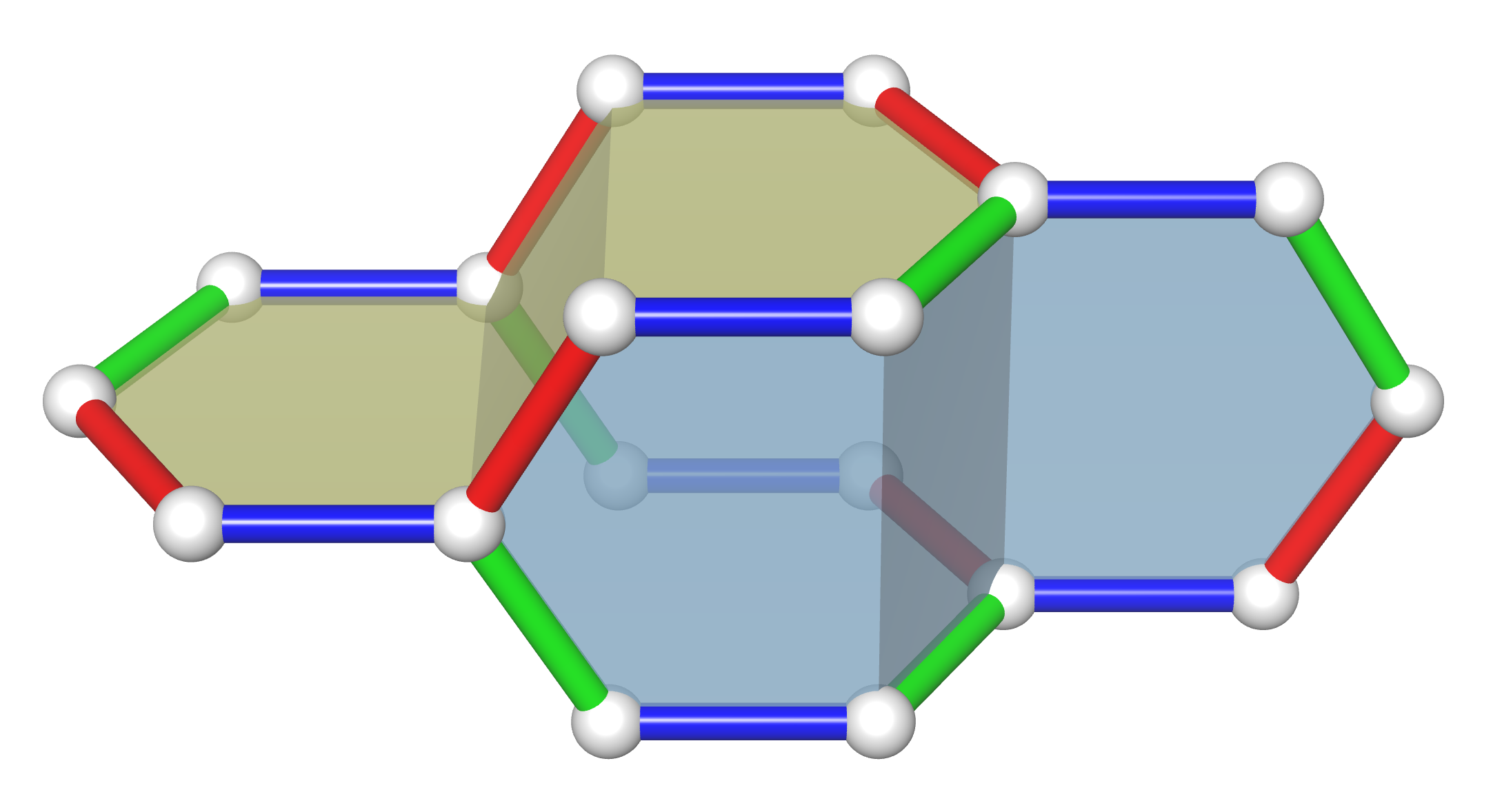
Figure 7: Part of (10,3)-$b$ including four loops forming a volume constraint. Two elementary loops with different coloring patterns are highlighted by yellow and cyan surfaces, respectively.

Among various point group symmetries, the inversion symmetry of the lattice is the most useful. As is the case in the honeycomb lattice, if an elementary loop has an inversion center, then the flux inside this loop becomes the square of some Pauli matrices times a complex number, which actually only takes $1,i,-1,-i.$ Therefore, the existence of an inversion center automatically proves that the flux is Abelian and should be $0$ or $\pi.$ This is another proof that a non-Abelian flux vanishes on some lattices. This applies, for example, to the hyperhoneycomb lattice (10,3)-$b.$ All the four elementary loops of length 10 (10-loops) have an inversion center, making the direct calculation easier. We can classify these four 10-loops into two pairs, where two loops are related by the glide mirror symmetry with the same coloring pattern for each pair. Therefore, it is enough to check two loops, shown in the yellow and cyan surfaces, respectively, in Fig. 7.

$$U^{b}U^{c}U^{a}U^{c}U^{a}U^{b}U^{c}U^{a}U^{c}U^{a} =I_{4}.$$ (42)

$$U^{a}U^{c}U^{b}U^{c}U^{b}U^{a}U^{c}U^{b}U^{c}U^{b} =I_{4}.$$ (43)

Therefore, all the four elementary loops in (10,3)-$b$ have a zero flux.

E.3 (10,3)-$d$

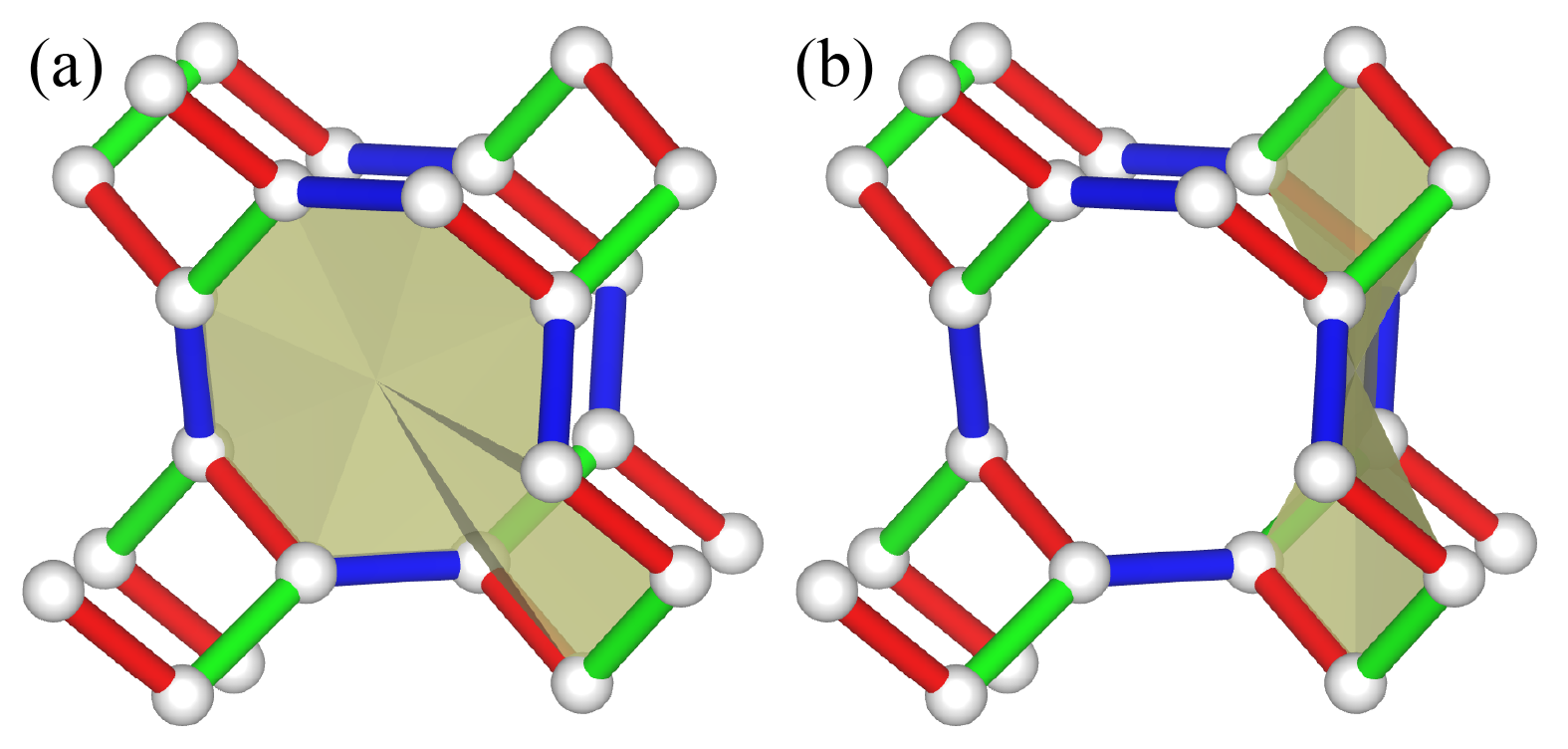
Figure 8: Part of (10,3)-$d.$ (a) One of the type-A loops highlighted by the yellow surface. (b) One of the type-B loops highlighted by the yellow surface.

The structure of (10,3)-$d$ is related to (10,3)-$a$ because they share the same projection onto the (001) plane, the 2D squareoctagon lattice. Due to the difference in the chiralities of the square spirals, the unit cell is enlarged in (10,3)-$d$ and possess 8 elementary loops (of length 10) per unit cell.

Since this lattice does not allow any 120-degree configuration, we cannot simply decide the bond coloring. If we take the most symmetric bond coloring discussed in Yamada et al. (2017), then the calculation becomes simple. We can divide 8 elementary loops of length 10 into two types. Four type-A loops are spiraling up the octagon spiral and then spiraling down the square spiral [see Fig. 8(a)]. All the four type-A loops are related by the inversion symmetry or the twofold screw rotation symmetry (the combination of them is the glide mirror symmetry), and thus have the same flux. Four type-B loops are spiraling up the square spiral and then spiraling down the nearest-neighbor square spiral [see Fig. 8(b)]. Four type-B loops are related by the twofold screw rotation symmetry or by the glide mirror symmetry, and have the same flux. Thus, it is enough to check one for each type.

$$U^{b}U^{c}U^{a}U^{c}U^{a}U^{b}U^{a}U^{c}U^{a}U^{c} =I_{4}.$$ (44)

$$U^{b}U^{a}U^{b}U^{a}U^{c}U^{b}U^{a}U^{b}U^{a}U^{c} =I_{4}.$$ (45)

The direct calculation tells us that the hopping model is in a zero-flux configuration.

E.4 $8^{2}.10$-$a$

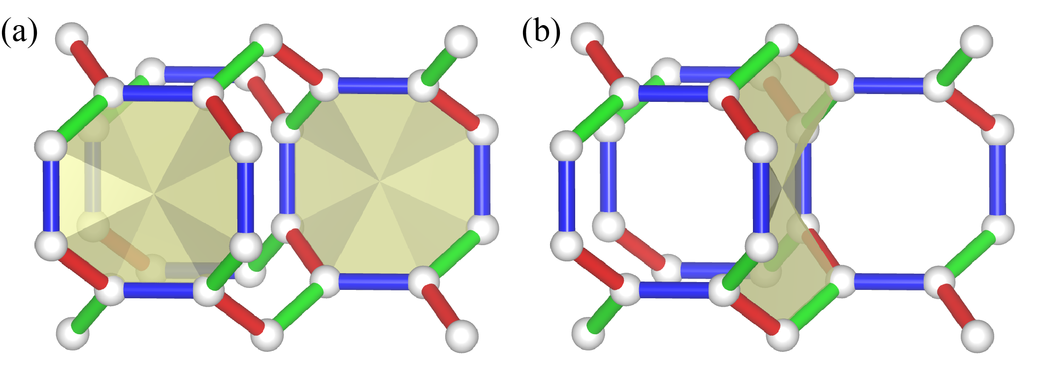
Figure 9: Part of $8^{2}.10$-$a.$ (a) All the two 8-loops are shown by yellow surfaces. They are related by the fourfold screw rotation symmetry. (b) One of the four 10-loops is shown by the yellow surface. The rest are produced by applying the fourfold screw rotation around the square spiral.

$8^{2}.10$-$a$ is nonuniform, but Archimedean. Therefore, each site is included in the two types of elementary loops, some of length 8 and others of length 10. The unit cell includes two elementary loops of length 8 (8-loops) [see Fig. 9(a)] and four elementary loops of length 10 (10-loops) [see Fig. 9(b)]. It is enough to check one of the 8-loops and one of the 10-loops because all the elementary loops of the same length are related by the fourfold screw rotation symmetry.

$$U^{a}U^{c}U^{b}U^{c}U^{a}U^{c}U^{b}U^{c} =-I_{4}.$$ (46)

$$U^{c}U^{a}U^{b}U^{a}U^{b}U^{c}U^{a}U^{b}U^{a}U^{b} =I_{4}.$$ (47)

Therefore, all the 8-loops have a $\pi$ flux and all the 10-loops have a zero flux. We note that the hopping model in this $\pi$-flux configuration does not break the original translation symmetry Yamada et al. (2017).

E.5 (8,3)-$b$

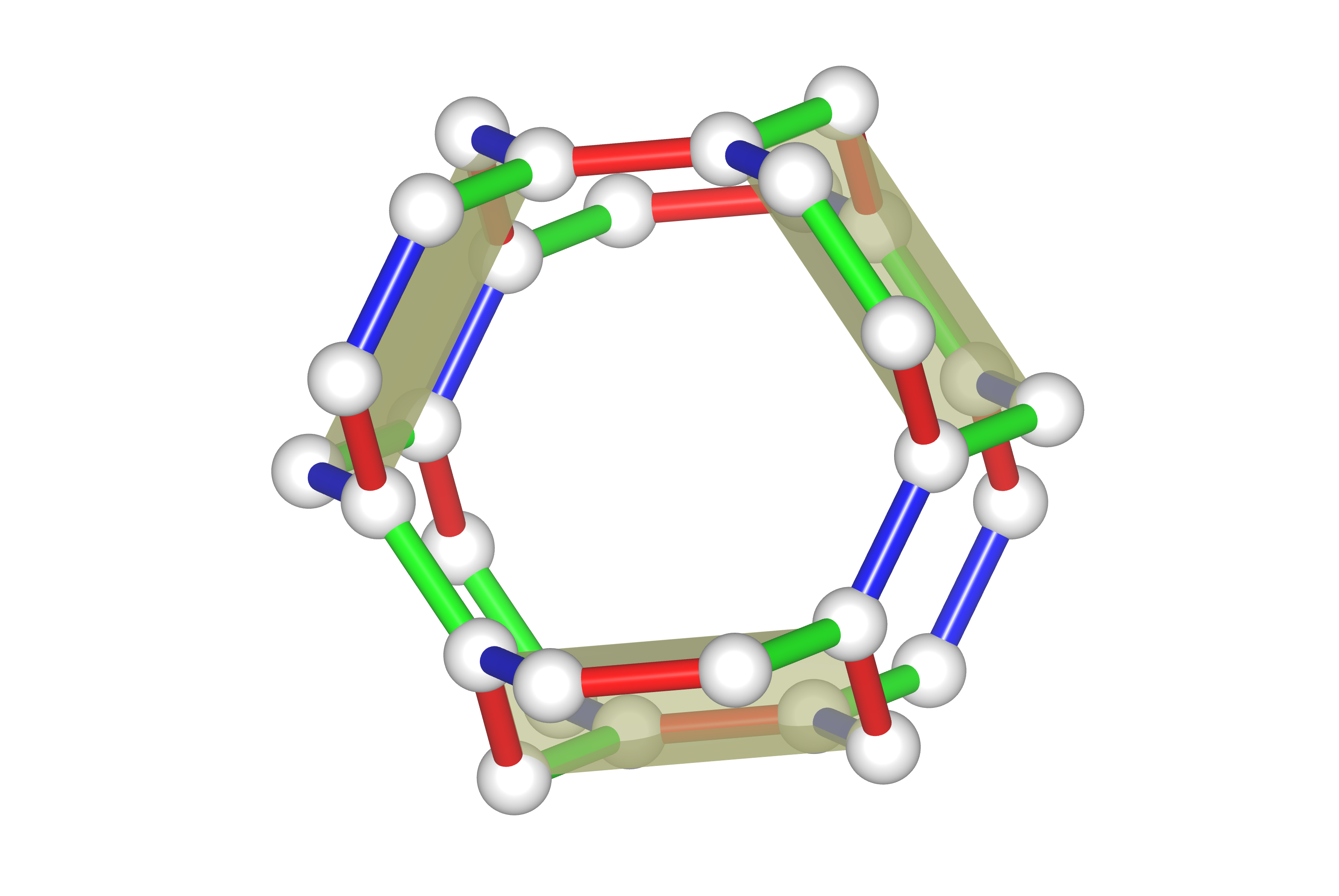
Figure 10: Part of (8,3)-$b.$ All the three elementary loops of length 8 are highlighted by yellow surfaces. They are related by the threefold rotation symmetry.

The hyperhexagon lattice (8,3)-$b$ has three elementary loops of length 8, and they are related by the threefold rotation symmetry changing the $xyz$-axes, as shown in Fig. 10. Therefore, it is enough to check only one of them. The direct calculation tells us that it has a $\pi$ flux.

$$U^{a}U^{c}U^{b}U^{c}U^{a}U^{c}U^{b}U^{c}=-I_{4}.$$ (48)

Therefore, (8,3)-$b$ is in the $\pi$-flux configuration. We note that there is another elementary loop of length 12, but the flux value is immediately determined to be zero due to the accidental fourfold symmetry of the coloring. It is worth mentioning the hopping model in this $\pi$-flux configuration does not break the original translation symmetry, and thus the LSMA theorem applies as it is to the $\pi$-flux $\mathrm{SU}(4)$ Hubbard model, as well as the $\mathrm{SU}(4)$ Heisenberg model.

E.6 Stripyhoneycomb lattice

The stripyhoneycomb lattice is nonuniform, so the length of the shortest elementary loops differs in space. Every elementary loop of length 6 is the same as the honeycomb, and thus has a $\pi$ flux. The structure includes two types of the $\pi$-flux hexagons aligning in different planes Kimchi et al. (2014). In addition, there exist a long loop of length 14 (14-loop) and a twisted loop of length 12 (12-loop) [see Fig. 11]. These four types of elementary loops are enough to determine the flux values.

One 14-loop shown in Fig. 11(a) has a zero flux because

$$U^{a}U^{c}U^{a}U^{b}U^{c}U^{b}U^{c}U^{a}U^{c}U^{a}U^{b}U^{c}U^{b}U^{c}=I_{4}.$$ (49)

One 12-loop shown on the right-hand side of Fig. 11(b) also has a zero flux because

$$U^{a}U^{b}U^{c}U^{a}U^{b}U^{c}U^{b}U^{a}U^{c}U^{b}U^{a}U^{c}=I_{4}.$$ (50)

There are many other tricoordinated lattices not discussed in this paper, so it is future work to determine the flux values for all the possible tricoordinated lattices.

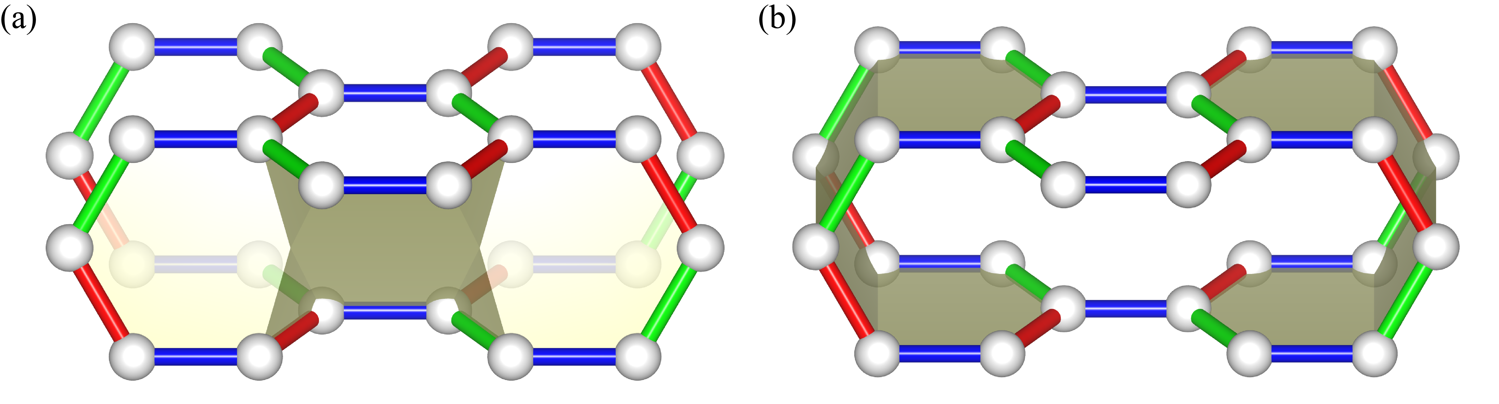
Figure 11: Part of the stripyhoneycomb lattice. (a) A loop of length 14 is highlighted. (b) A pair of loops of length 12 are highlighted. They are related by the inversion symmetry (or the volume constraint) and thus have the same flux.

References

- Yamada et al. (2018) Masahiko G. Yamada, Masaki Oshikawa, and George Jackeli, “Emergent symmetry in - and crystalline spin-orbital liquids,” Phys. Rev. Lett. 121, 097201 (2018).
- Natori et al. (2018) Willian M. H. Natori, Eric C. Andrade, and Rodrigo G. Pereira, “Su(4)-symmetric spin-orbital liquids on the hyperhoneycomb lattice,” Phys. Rev. B 98, 195113 (2018).
- Cazalilla and Rey (2014) Miguel A Cazalilla and Ana Maria Rey, “Ultracold fermi gases with emergent SU(n) symmetry,” Rep. Prog. Phys. 77, 124401 (2014).
- Corboz et al. (2012) Philippe Corboz, Miklós Lajkó, Andreas M. Läuchli, Karlo Penc, and Frédéric Mila, “Spin-orbital quantum liquid on the honeycomb lattice,” Phys. Rev. X 2, 041013 (2012).
- Kitaev (2006) Alexei Kitaev, “Anyons in an exactly solved model and beyond,” Ann. Phys. 321, 2–111 (2006), january Special Issue.
- Saitoh et al. (2001) E. Saitoh, S. Okamoto, K. T. Takahashi, K. Tobe, K. Yamamoto, T. Kimura, S. Ishihara, S. Maekawa, and Y. Tokura, “Observation of orbital waves as elementary excitations in a solid,” Nature 410, 180–183 (2001).
- Tokura and Nagaosa (2000) Y. Tokura and N. Nagaosa, “Orbital physics in transition-metal oxides,” Science 288, 462–468 (2000), https://science.sciencemag.org/content/288/5465/462.full.pdf .
- Kugel and Khomskii (1982) Kliment I. Kugel and D. I. Khomskii, “The jahn-teller effect and magnetism: transition metal compounds,” Sov. Phys. Usp. 25, 231 (1982).
- Zhou et al. (2011) H. D. Zhou, E. S. Choi, G. Li, L. Balicas, C. R. Wiebe, Y. Qiu, J. R. D. Copley, and J. S. Gardner, “Spin liquid state in the triangular lattice ,” Phys. Rev. Lett. 106, 147204 (2011).
- Nakatsuji et al. (2012) S. Nakatsuji, K. Kuga, K. Kimura, R. Satake, N. Katayama, E. Nishibori, H. Sawa, R. Ishii, M. Hagiwara, F. Bridges, T. U. Ito, W. Higemoto, Y. Karaki, M. Halim, A. A. Nugroho, J. A. Rodriguez-Rivera, M. A. Green, and C. Broholm, “Spin-orbital short-range order on a honeycomb-based lattice,” Science 336, 559–563 (2012).
- Smerald and Mila (2014) Andrew Smerald and Frédéric Mila, “Exploring the spin-orbital ground state of ,” Phys. Rev. B 90, 094422 (2014).
- Ohkawa (1983) Fusayoshi J. Ohkawa, “Ordered states in periodic anderson hamiltonian with orbital degeneracy and with large coulomb correlation,” J. Phys. Soc. Jpn. 52, 3897–3906 (1983).
- Shiina et al. (1997) Ryousuke Shiina, Hiroyuki Shiba, and Peter Thalmeier, “Magnetic-field effects on quadrupolar ordering in a -quartet system ceb6,” J. Phys. Soc. Jpn. 66, 1741–1755 (1997).
- Wang and Vishwanath (2009) Fa Wang and Ashvin Vishwanath, “ spin-orbital liquid state in the square lattice kugel-khomskii model,” Phys. Rev. B 80, 064413 (2009).
- Kugel et al. (2015) K. I. Kugel, D. I. Khomskii, A. O. Sboychakov, and S. V. Streltsov, “Spin-orbital interaction for face-sharing octahedra: Realization of a highly symmetric su(4) model,” Phys. Rev. B 91, 155125 (2015).
- Xu and Balents (2018) Cenke Xu and Leon Balents, “Topological superconductivity in twisted multilayer graphene,” Phys. Rev. Lett. 121, 087001 (2018).
- Zhu et al. (2019) Zheng Zhu, D. N. Sheng, and Liang Fu, “Spin-orbital density wave and a mott insulator in a two-orbital hubbard model on a honeycomb lattice,” Phys. Rev. Lett. 123, 087602 (2019).
- Wen (2002) Xiao-Gang Wen, “Quantum orders and symmetric spin liquids,” Phys. Rev. B 65, 165113 (2002).
- Affleck and Marston (1988) Ian Affleck and J. Brad Marston, “Large- limit of the heisenberg-hubbard model: Implications for high- superconductors,” Phys. Rev. B 37, 3774–3777 (1988).
- Calvera and Wang (2021) Vladimir Calvera and Chong Wang, “Theory of dirac spin-orbital liquids: monopoles, anomalies, and applications to honeycomb models,” (2021), arXiv:2103.13405 [cond-mat.str-el] .
- Takayama et al. (2015) T. Takayama, A. Kato, R. Dinnebier, J. Nuss, H. Kono, L. S. I. Veiga, G. Fabbris, D. Haskel, and H. Takagi, “Hyperhoneycomb iridate as a platform for kitaev magnetism,” Phys. Rev. Lett. 114, 077202 (2015).
- Lieb (1994) Elliott H. Lieb, “Flux phase of the half-filled band,” Phys. Rev. Lett. 73, 2158–2161 (1994).
- Keselman et al. (2020) Anna Keselman, Bela Bauer, Cenke Xu, and Chao-Ming Jian, “Emergent fermi surface in a triangular-lattice su(4) quantum antiferromagnet,” Phys. Rev. Lett. 125, 117202 (2020).
- Jin et al. (2021) Hui-Ke Jin, Rong-Yang Sun, Hong-Hao Tu, and Yi Zhou, “Unveiling critical stripy state in the triangular-lattice su(4) spin-orbital model,” (2021), arXiv:2106.09318 [cond-mat.str-el] .
- Azaria et al. (1999) P. Azaria, A. O. Gogolin, P. Lecheminant, and A. A. Nersesyan, “One-dimensional su(4) spin-orbital model: A low-energy effective theory,” Phys. Rev. Lett. 83, 624–627 (1999).
- Corboz et al. (2011) Philippe Corboz, Andreas M. Läuchli, Karlo Penc, Matthias Troyer, and Frédéric Mila, “Simultaneous dimerization and su(4) symmetry breaking of 4-color fermions on the square lattice,” Phys. Rev. Lett. 107, 215301 (2011).
- Swaroop and Flengas (1964a) B. Swaroop and S. N. Flengas, “The synthesis of anhydrous zirconium trichloride,” Can. J. Chem. 42, 1495–1498 (1964a).
- Swaroop and Flengas (1964b) B. Swaroop and S. N. Flengas, “Crystal structure of zirconium trichloride,” Can. J. Phys. 42, 1886–1889 (1964b).
- Daake and Corbett (1978) Richard L. Daake and John D. Corbett, “Synthesis and nonstoichiometry of the zirconium trihalides,” Inorg. Chem. 17, 1192–1195 (1978).
- Ushakov et al. (2020) A. V. Ushakov, I. V. Solovyev, and S. V. Streltsov, “Can the highly symmetric su(4) spin-orbital model be realized in -zrcl3?” Pis’ma Zh. Eksp. Teor. Fiz. 112, 686 (2020).
- Plumb et al. (2014) K. W. Plumb, J. P. Clancy, L. J. Sandilands, V. Vijay Shankar, Y. F. Hu, K. S. Burch, Hae-Young Kee, and Young-June Kim, “-: A spin-orbit assisted mott insulator on a honeycomb lattice,” Phys. Rev. B 90, 041112 (2014).
- Note (1) The Cartesian axes are defined as shown in Fig. 3(b).
- Lieb et al. (1961) Elliott Lieb, Theodore Schultz, and Daniel Mattis, “Two soluble models of an antiferromagnetic chain,” Ann. Phys. 16, 407–466 (1961).
- Affleck and Lieb (1986) Ian Affleck and Elliott H. Lieb, “A proof of part of haldane’s conjecture on spin chains,” Lett. Math. Phys. 12, 57–69 (1986).
- Lajkó et al. (2017) Miklós Lajkó, Kyle Wamer, Frédéric Mila, and Ian Affleck, “Generalization of the haldane conjecture to su(3) chains,” Nucl. Phys. B 924, 508 – 577 (2017).
- Yao et al. (2019) Yuan Yao, Chang-Tse Hsieh, and Masaki Oshikawa, “Anomaly matching and symmetry-protected critical phases in spin systems in dimensions,” Phys. Rev. Lett. 123, 180201 (2019).
- Affleck (1988) Ian Affleck, “Spin gap and symmetry breaking in layers and other antiferromagnets,” Phys. Rev. B 37, 5186–5192 (1988).
- Oshikawa (2000) Masaki Oshikawa, “Commensurability, excitation gap, and topology in quantum many-particle systems on a periodic lattice,” Phys. Rev. Lett. 84, 1535–1538 (2000).
- Hastings (2005) M. B. Hastings, “Sufficient conditions for topological order in insulators,” Europhys. Lett. 70, 824 (2005).
- (40) K. Totsuka, “Lieb-Schultz-Mattis approach to SU()-symmetric Mott insulators,” JPS 72nd Annual Meeting (2017).
- Jian and Zaletel (2016) Chao-Ming Jian and Michael Zaletel, “Existence of featureless paramagnets on the square and the honeycomb lattices in 2+1 dimensions,” Phys. Rev. B 93, 035114 (2016).
- Lu et al. (2020) Yuan-Ming Lu, Ying Ran, and Masaki Oshikawa, “Filling-enforced constraint on the quantized hall conductivity on a periodic lattice,” Ann. Phys. , 168060 (2020).
- Hermanns et al. (2015a) M. Hermanns, K. O’Brien, and S. Trebst, “Weyl spin liquids,” Phys. Rev. Lett. 114, 157202 (2015a).
- Hermanns et al. (2015b) Maria Hermanns, Simon Trebst, and Achim Rosch, “Spin-peierls instability of three-dimensional spin liquids with majorana fermi surfaces,” Phys. Rev. Lett. 115, 177205 (2015b).
- O’Brien et al. (2016) Kevin O’Brien, Maria Hermanns, and Simon Trebst, “Classification of gapless spin liquids in three-dimensional kitaev models,” Phys. Rev. B 93, 085101 (2016).
- Wells (1977) A. F. Wells, Three-dimensional Nets and Polyhedra (Wiley, New York, 1977).
- Rüdorff et al. (1956) W. Rüdorff, G. Walter, and H. Becker, “über einige oxoverbindungen und doppeloxyde des vierwertigen vanadins,” Z. Anorg. Allg. Chem. 285, 287–296 (1956).
- Modic et al. (2014) K. A. Modic, Tess E. Smidt, Itamar Kimchi, Nicholas P. Breznay, Alun Biffin, Sungkyun Choi, Roger D. Johnson, Radu Coldea, Pilanda Watkins-Curry, Gregory T. McCandless, Julia Y. Chan, Felipe Gandara, Z. Islam, Ashvin Vishwanath, Arkady Shekhter, Ross D. McDonald, and James G. Analytis, “Realization of a three-dimensional spin–anisotropic harmonic honeycomb iridate,” Nat. Commun. 5, 4203 (2014).
- Schrade and Fu (2019) Constantin Schrade and Liang Fu, “Spin-valley density wave in moiré materials,” Phys. Rev. B 100, 035413 (2019).
- Catuneanu et al. (2015) Andrei Catuneanu, Jeffrey G. Rau, Heung-Sik Kim, and Hae-Young Kee, “Magnetic orders proximal to the kitaev limit in frustrated triangular systems: Application to ,” Phys. Rev. B 92, 165108 (2015).
- Law and Lee (2017) K. T. Law and Patrick A. Lee, “1t-tas2 as a quantum spin liquid,” Proc. Natl. Acad. Sci. USA 114, 6996–7000 (2017), https://www.pnas.org/content/114/27/6996.full.pdf .
- Yu et al. (2017) Y. J. Yu, Y. Xu, L. P. He, M. Kratochvilova, Y. Y. Huang, J. M. Ni, Lihai Wang, Sang-Wook Cheong, Je-Geun Park, and S. Y. Li, “Heat transport study of the spin liquid candidate ,” Phys. Rev. B 96, 081111 (2017).
- Murayama et al. (2020) H. Murayama, Y. Sato, T. Taniguchi, R. Kurihara, X. Z. Xing, W. Huang, S. Kasahara, Y. Kasahara, I. Kimchi, M. Yoshida, Y. Iwasa, Y. Mizukami, T. Shibauchi, M. Konczykowski, and Y. Matsuda, “Effect of quenched disorder on the quantum spin liquid state of the triangular-lattice antiferromagnet ,” Phys. Rev. Research 2, 013099 (2020).
- Assadi and Shigeta (2018) M. Hussein N. Assadi and Yasuteru Shigeta, “The effect of octahedral distortions on the electronic properties and magnetic interactions in o3 natmo2 compounds (tm = ti–ni & zr–pd),” RSC Adv. 8, 13842–13849 (2018).
- Singh et al. (2004) S. P. Singh, M. Tomar, Yasuyuki Ishikawa, S. B. Majumder, and R. S. Katiyar, “Density-functional theoretical study on the intercalation properties of layered limo2 (m = zr, nb, rh, mo, and ru),” MRS Proc. 835, K6.3 (2004).
- Khaliullin and Maekawa (2000) G. Khaliullin and S. Maekawa, “Orbital liquid in three-dimensional mott insulator: ,” Phys. Rev. Lett. 85, 3950–3953 (2000).
- Han et al. (2015) Yibo Han, Masayuki Hagiwara, Takehito Nakano, Yasuo Nozue, Kenta Kimura, Mario Halim, and Satoru Nakatsuji, “Observation of the orbital quantum dynamics in the spin- hexagonal antiferromagnet ,” Phys. Rev. B 92, 180410 (2015).
- Nasu and Ishihara (2013) Joji Nasu and Sumio Ishihara, “Dynamical jahn-teller effect in a spin-orbital coupled system,” Phys. Rev. B 88, 094408 (2013).
- Nasu and Ishihara (2015) Joji Nasu and Sumio Ishihara, “Resonating valence-bond state in an orbitally degenerate quantum magnet with dynamical jahn-teller effect,” Phys. Rev. B 91, 045117 (2015).
- Bersuker (1975) I.B. Bersuker, “The jahn-teller effect in crystal chemistry and spectroscopy,” Coord. Chem. Rev. 14, 357 – 412 (1975).
- Abragam and Bleaney (1970) A. Abragam and B. Bleaney, Electron Paramagnetic Resonance of Transition Ions (Clarendon Press, Oxford, 1970).
- Romhányi et al. (2017) Judit Romhányi, Leon Balents, and George Jackeli, “Spin-orbit dimers and noncollinear phases in cubic double perovskites,” Phys. Rev. Lett. 118, 217202 (2017).
- Iwahara et al. (2017) Naoya Iwahara, Veacheslav Vieru, Liviu Ungur, and Liviu F. Chibotaru, “Zeeman interaction and jahn-teller effect in the multiplet,” Phys. Rev. B 96, 064416 (2017).
- Marrucci et al. (2006) L. Marrucci, C. Manzo, and D. Paparo, “Optical spin-to-orbital angular momentum conversion in inhomogeneous anisotropic media,” Phys. Rev. Lett. 96, 163905 (2006).
- Krämer et al. (1999) K. W. Krämer, H. U. Güdel, B. Roessli, P. Fischer, A. Dönni, N. Wada, F. Fauth, M. T. Fernandez-Diaz, and T. Hauss, “Noncollinear two- and three-dimensional magnetic ordering in the honeycomb lattices of (=cl,br,i),” Phys. Rev. B 60, R3724 (1999).
- Krämer et al. (2000) K. W. Krämer, H. U. Güdel, P. Fischer, F. Fauth, M. T. Fernandez-Diaz, and T. Hauß, “Triangular antiferromagnetic order in the honeycomb layer lattice of ercl3,” Eur. Phys. J. B 18, 39–47 (2000).
- Nataf et al. (2016) Pierre Nataf, Miklós Lajkó, Philippe Corboz, Andreas M. Läuchli, Karlo Penc, and Frédéric Mila, “Plaquette order in the su(6) heisenberg model on the honeycomb lattice,” Phys. Rev. B 93, 201113 (2016).
- Jain et al. (2013) Anubhav Jain, Shyue Ping Ong, Geoffroy Hautier, Wei Chen, William Davidson Richards, Stephen Dacek, Shreyas Cholia, Dan Gunter, David Skinner, Gerbrand Ceder, and Kristin a. Persson, “The Materials Project: A materials genome approach to accelerating materials innovation,” APL Materials 1, 011002 (2013).
- Momma and Izumi (2011) Koichi Momma and Fujio Izumi, “VESTA3 for three-dimensional visualization of crystal, volumetric and morphology data,” J. Appl. Crystallogr. 44, 1272–1276 (2011).
- Ogawa (1960) Shinji Ogawa, “Magnetic transition in ticl3,” J. Phys. Soc. Jpn. 15, 1901–1901 (1960).
- Jackeli and Ivanov (2007) G. Jackeli and D. A. Ivanov, “Dimer phases in quantum antiferromagnets with orbital degeneracy,” Phys. Rev. B 76, 132407 (2007).
- Normand and Oleś (2008) Bruce Normand and Andrzej M. Oleś, “Frustration and entanglement in the spin-orbital model on a triangular lattice: Valence-bond and generalized liquid states,” Phys. Rev. B 78, 094427 (2008).
- Chaloupka and Oleś (2011) Ji ří Chaloupka and Andrzej M. Oleś, “Spin-orbital resonating valence bond liquid on a triangular lattice: Evidence from finite-cluster diagonalization,” Phys. Rev. B 83, 094406 (2011).
- Georges et al. (2013) Antoine Georges, Luca de’ Medici, and Jernej Mravlje, “Strong correlations from hund’s coupling,” Annu. Rev. Condens. Matter Phys. 4, 137–178 (2013).
- Natori et al. (2019) W. M. H. Natori, R. Nutakki, R. G. Pereira, and E. C. Andrade, “Su(4) heisenberg model on the honeycomb lattice with exchange-frustrated perturbations: Implications for twistronics and mott insulators,” Phys. Rev. B 100, 205131 (2019).
- Yamada et al. (2017) Masahiko G. Yamada, Vatsal Dwivedi, and Maria Hermanns, “Crystalline kitaev spin liquids,” Phys. Rev. B 96, 155107 (2017).
- Watanabe et al. (2015) Haruki Watanabe, Hoi Chun Po, Ashvin Vishwanath, and Michael Zaletel, “Filling constraints for spin-orbit coupled insulators in symmorphic and nonsymmorphic crystals,” Proc. Natl. Acad. Sci. USA 112, 14551–14556 (2015).
- Parameswaran et al. (2013) Siddharth A. Parameswaran, Ari M. Turner, Daniel P. Arovas, and Ashvin Vishwanath, “Topological order and absence of band insulators at integer filling in non-symmorphic crystals,” Nat. Phys. 9, 299–303 (2013).
- Po et al. (2017) Hoi Chun Po, Haruki Watanabe, Chao-Ming Jian, and Michael P. Zaletel, “Lattice homotopy constraints on phases of quantum magnets,” Phys. Rev. Lett. 119, 127202 (2017).
- König and Mermin (1999) Anja König and N. David Mermin, “Screw rotations and glide mirrors: Crystallography in fourier space,” Proc. Natl. Acad. Sci. USA 96, 3502–3506 (1999).
- Note (2) We can show that if is an integer, then this nonsymmorphic operation is removable, i.e. can be reduced to a point-group operation times a lattice translation by change of origin König and Mermin (1999).
- Delgado Friedrichs et al. (2003a) Olaf Delgado Friedrichs, Michael O’Keeffe, and Omar M. Yaghi, “Three-periodic nets and tilings: regular and quasiregular nets,” Acta Crystallogr. Sect. A 59, 22–27 (2003a).
- Delgado Friedrichs et al. (2003b) Olaf Delgado Friedrichs, Michael O’Keeffe, and Omar M. Yaghi, “Three-periodic nets and tilings: semiregular nets,” Acta Crystallogr. Sect. A 59, 515–525 (2003b).
- Hermanns and Trebst (2014) M. Hermanns and S. Trebst, “Quantum spin liquid with a majorana fermi surface on the three-dimensional hyperoctagon lattice,” Phys. Rev. B 89, 235102 (2014).
- Kimchi et al. (2014) Itamar Kimchi, James G. Analytis, and Ashvin Vishwanath, “Three-dimensional quantum spin liquids in models of harmonic-honeycomb iridates and phase diagram in an infinite- approximation,” Phys. Rev. B 90, 205126 (2014).