Features of the Primordial Universe in $f(R)$-gravity as viewed in the Jordan frame

Abstract

We analyze some relevant features of the primordial Universe as viewed in the Jordan frame formulation of the $f(R)$-gravity, especially when the potential term of the non-minimally coupled scalar field is negligible. We start formulating the Hamiltonian picture in the Jordan frame, using the 3-metric determinant as a basic variable and we outline that its conjugated momentum appears linearly only in the scalar constraint. Then, we construct the basic formalism to characterize the dynamics of a generic inhomogeneous cosmological model and specialize it in order to describe behaviors of the Bianchi Universes, both on a classical and a quantum regime. As a fundamental issue, we demonstrate that, when the potential term of the additional scalar mode is negligible near enough to the initial singularity, the Bianchi IX cosmology is no longer affected by the chaotic behavior, typical in vacuum of the standard Einsteinian dynamics. In fact, the presence of stable Kasner stability region and its actractive character are properly characterized. Finally, we investigate the canonical quantization of the Bianchi I model, using as time variable the non-minimally coupled scalar field and showing that the existence of a conserved current is outlined for the corresponding Wheeler-DeWitt equation. The behavior of a localized wave-packet for the isotropic Universe is also evolved, demonstrating that the singularity is still present in this revised quantum dynamics.

Part I Introduction

The Standard Cosmological Model [1], which provides a consistent and probed general picture of the Universe thermal history, at least after a post-inflationary temperature (but also the inflationary model is a reliable theoretical framework with observational favourable indications) is entirely based on the standard Einsteinian formulation of the gravitational field (also the Standard Model of elementary particles has a fundamental role). However, it is a well-know fact that, at very primordial instants (say pre-inflationary age) its nature can be more complicated than the simple isotropic model and additional effects from modified and quantum gravity can become important [2, 3, 4]. The most natural generalization of the isotropic Robertson geometry is provided by [5, 3]. In particular, the Bianchi type VIII and IX cosmological models (the most general allowed by the homogeneity constraint) have an Einsteinian chaotic dynamics, which constitutes a valuable prototype for the asymptotic behavior to the singularity of the generic inhomogeneous universe (no space symmetries are imposed) [6, 7, 3]. Furthermore it must be noted that, while the kinematic structure of General Relativity (namely its covariant nature) expressed via the tensor language is a solid theoretical construction, the Einstein equations are not very general in their derivation. In fact, the Einsteinian dynamics is fixed by the simplest scalar action (the Einstein-Hilbert action), having the special feature of being the only one to provide field equations with second derivatives of the metric tensor only. More general formulation for the gravitational field dynamics can be easily constructed by very general scalar Lagrangian [8]. Among the possible restatements of the gravitational dynamics, it stands out for its simplicity and its capability to explain phenomena like dark matter and, overall, the so-called $f(R)$ model, whose Lagrangian is a function of the Ricci scalar. The interest for this model relies also in the possibility to restate the $f(R)$ model in terms of a scalar-tensor formulation, in which a scalar field is non-minimally coupled to standard gravity in the so-called Jordan frame or minimally coupled to it in the so-called Einstein frame [8, 9]. We finally observe that the canonical quantization of the gravitational field is also an open problem in the $f(R)$ model, calling attention as in the case of ordinary Einsteinian gravity. In fact, the idea that the corrections to the Einstein-Hilbert action must be relevant when the Universe density overcome the nuclear density and, more in general, near enough to the initial singularity, must be conjugated with the idea that, in the same limit, at Planckian scales, the quantum dynamics of the gravitational field is a mandatory description. In this paper, we provide a general discussion of the primordial Universe in the $f(R)$ formulation of the gravitational field, as viewed in the Jordan frame, facing both symmetric and generic models, as well as both classical and quantum effects; for related topics see [10, 11, 12, 13]. We start by re-analyzing the study presented in [14], in which the Hamiltonian formulation of the $f(R)$ gravitational dynamics in the Jordan frame is developed. In particular, we introduce a representation of the 3-metric tensor in which the 3-determinant is isolated, like in the original analysis in [15]. Thus, we outline that the conjugate momentum to the 3-determinant enters linearly only in the gravitational Hamiltonian. Considerations on the structure of the corresponding Wheeler-DeWitt equation are developed, clarifying how it seems to resembles the morphology of a Schröedinger functional equation (although non-local) than a Klein-Gordon functional equation as in standard gravity [2] with respect to the choice of the 3-determinant as time variable. On the base of the general formulation above traced, we consider the formulation of a generic cosmological model in the Jordan frame, generalizing similar studies developed in Einsteinian gravity, see [16, 17, 18, 19]. Then, we specialize this scheme to the symmetric case of the homogeneous but anisotropic Bianchi universes, for which we construct the generic Hamiltonian picture, then focusing attention to the Bianchi I and Bianchi IX models. Here we provide a detailed analysis of the Bianchi IX universe, demonstrating that, as far as the potential term of the non-minimally coupled scalar field (depending on the form of $f$ ) is negligible, the chaos of the standard gravitational dynamics in vacuum is removed. We outline the existence of the so-called generalized Kasner solution and, via a numerical analysis, we show its actractivity during the system evolution. Finally, we face the treatment of quantum features of the $f(R)$ gravity in the Jordan frame, by implementing the Dirac canonical method to the restated Hamiltonian constraints. We pay attention on the Bianchi I cosmological model, constructing a conserved current for the associated Wheeler-DeWitt equation. The construction of an evolutive wave packet is limited to the isotropic case only, being that, if the non-minimally coupled scalar field potential is negligible, the singularity still appears in the generalized quantum gravity framework of the Jordan frame, having chosen such a field as the system internal time. The comparison with the case of the standard Einsteinian isotropic quantum Universe in the presence of a minimally coupled scalar field as a matter clock is finally provided. The manuscript is organized as follows. In Part II we present the $f(R)$ theories of gravity in the so-called Jordan frame. We also introduce the $f(R)$ Hamiltonian formalism and then we quantize it using the Dirac scheme. In Part III we provide a general picture of the Bianchi classification, focusing our attention on the Kasner solution for Bianchi I Universe in standard General Relativity and on the Bianchi IX universe. We underline its chaotic behaviour and characterize its evolution as we approaching to cosmological singularity. In Part IV we deal with the formalism of the generic cosmological problem of the $f(R)$ theories in the Jordan frame. In Part V we analyze the features of classical $f(R)$ cosmology. We derive Kasner solutions and then we use them to determine the conditions for which the scalar field potential is negligible. We also perform an analysis of the Bianchi IX cosmology showing the attractivity of the stability region. In Part VI we perform a critical study on the canonical quantization of the Bianchi I model and of the homogeneous and isotropic Universe (FLRW) in the case of the $f(R)$ theories of gravity in the Jordan frame. In particular, using the non-minimally coupled scalar field as a quantum time, we carry out an analysis on the quantum dynamics of the FLRW model and finally we make a comparison with the case of a minimally coupled external scalar field in General Relativity. In Part VII concluding remarks follow.

Part II $f(R)$ gravity

The Einstein’s theory of General Relativity represents the current classical theory of gravity. Its geometrical and tensorial structure determines the kinematics of the gravitational field in a very consistent formulation, but its dynamics admits a wide class of different proposals. In fact the Einstein-Hilbert Lagrangian $\mathcal{L}_{EH}=R$, proposed by Hilbert in 1915, is only the most simple proposal. The Ricci scalar $R$ depends on the second derivatives of the metric tensor $g_{\mu\nu}$ and the corresponding field equations constitute a system of second order differential equations with respect to the metric tensor $g_{\mu\nu}$, in full coherence with the ”aesthetic request” of the late 19th century to have a physical theory containing at most second-order derivatives of potentials. Even the choice of a covariant Lagrangian is not mandatory. In fact, for the equation of motions to be covariant, the covariance of the action functional is just a sufficient but not necessary condition.

I The Jordan frame

A more general formulation of the gravitational field dynamics consists in the replacement of the Ricci scalar by a generic function $f(R)$. In the $f(R)$ theories of gravity, proposed by Buchdal in 1970, the corresponding action of the gravitational field takes the form

$$S_{g}=\cfrac{1}{2k}\int d^{4}x\sqrt{-g}\,f(R),$$ (1)

where $k=8\pi Gc^{-4}$ and $-g$ is the positive determinant of the metric tensor $g_{\mu\nu}$. In this way, a new geometric degree of freedom is included in the theory (the function $f$), which induces different field equations [8]. There are actually three possible variational principles that one can apply in order to derive the Einstein’s field equations . In the following, we will refer exclusively to the metric formalism. Beginning from the action (1) and adding a matter term $S_{M}$, the total action for $f(R)$ gravity takes the form

$$S=\cfrac{1}{2k}\int d^{4}x\sqrt{-g}f(R)+S_{M}\left(g_{\mu\nu},\psi\right),$$ (2)

where $\psi$ denotes a generic matter field.

In a field theory it is always possible to perform redefinitions of the fields, in order to rewrite the action and the equations in a more convenient way. If the new action coincides with the previous one, the two theories are said to be dynamically equivalent and they are actually just different representations of the same theory. In what follows, we will show the equivalence between the metric $f(R)$ gravity theory and a specific theory within the Brans-Dicke class. One can introduce an auxiliary field $A$ and rewrite the action (2) as

$$S=\cfrac{1}{2k}\int d^{4}x\sqrt{-g}\left[f(A)+f^{\prime}(A)(R-A)\right]+S_{M}.$$ (3)

Variation with respect to $A$ leads to the equation

$$f^{\prime\prime}(A)\left(R-A\right)=0.$$ (4)

Therefore, if $f^{\prime\prime}(A)\neq 0$ we obtain the result $A=R$ and by substitution in the action (3) we find the dinamically equivalent action (2). We now redefine the field $A$ by introducing the scalar field $\phi=f^{\prime}(A)$ and its potential $V\left(\phi\right)=A(\phi)\phi-f\left(A(\phi)\right)$. In this way the action (3) takes the form

$$S=\cfrac{1}{2k}\int d^{4}x\sqrt{-g}\left[\phi R-V(\phi)\right]+S_{M}\left(g_{\mu\nu},\psi\right).$$ (5)

This is the Jordan frame representation of the action of a Brans–Dicke theory with Brans–Dicke parameter $\omega_{0}=0$. Action (5) is also known as the $f(R)$ gravitational action in the Jordan frame. It is the scalar-tensor equivalent representation of the action (2), expressed through a non-minimal coupling between a scalar field $\left(\phi\right)$ and the curvature $\left(R\right)$.

II Jordan frame Hamiltonian of $f(R)$ gravity

In this section we will review the Arnowitt-Deser-Misner Hamiltonian formulation of $f(R)$ gravity in the Jordan frame using the embedding technique. Consider a four dimension spacetime $\mathcal{M}^{4}$ diffeomorphic to a manifold $\mathbb{R}\text{\texttimes}\Sigma^{3}$, allowing the splitting $\mathcal{M}^{4}=\mathbb{R}\text{\texttimes}\Sigma^{3}$. In this way $\mathcal{M}^{4}$ can be foliated by a one-parameter family of space-like 3-hypersurfaces $\Sigma_{t}^{3}$, embedded in the ambient spacetime and defined by mean a temporal scalar parameter $t$. We introduce the extrinsic curvature

$$K_{ij}=\frac{1}{2N}\left(D_{i}N_{j}+D_{j}N_{i}-\partial_{t}h_{ij}\right),$$ (6)

where $D_{i}$ ($i=1,2,3$ spatial indices) is the covariant derivative associated to the 3-metric $h_{ij}$ induced on each $\varSigma_{t}$. The Ricci scalar can be written in terms of the ADM variables $\left(N,N^{i},h_{ij},t\right)$ through the so-called Gauss-Codazzi equation

$$R =\,_{T}K.\,_{T}K-\frac{2}{3}K^{2}+$$

$$\quad+\,^{3}R+\frac{2}{\sqrt{-g}}\partial_{\mu}\left(\sqrt{-g}n^{\mu}K\right)$$

$$\quad-\frac{2}{N\sqrt{h}}\partial_{i}\left(\sqrt{h}h^{ij}\partial_{j}N\right),$$ (7)

where ${}^{3}R\left(h_{ij},\partial_{l}h_{ij},\partial_{m}\partial_{l}h_{ij}\right)$ is the Ricci 3-scalar, $\,{}_{T}K_{ij}=\left(K_{ij}-\frac{1}{3}h_{ij}K\right)$ ; $\,{}_{T}K.\,_{T}K=\,_{T}K_{ij}\,{}_{T}K^{ij}$ and $h=det\left(h_{ij}\right)$. Substituting the relation (7) in the total Action (5) and neglecting the matter term $S_{M}$, we obtain the ADM action of $f(R)$ gravity in the Jordan frame (with $k\equiv 1)$

$$\begin{array}[]{l}S_{JF}^{ADM}\left(h_{ij},N,N^{i},\phi\right)=\\ \int_{\mathbb{R}\text{\texttimes}\Sigma}dtd^{3}xN\sqrt{h}\Biggl{[}\cfrac{\phi}{2}\left(\,{}_{T}K.\,_{T}K-\frac{2}{3}K^{2}+\,^{3}R\right)-\cfrac{1}{2}V\left(\phi\right)\\ -\cfrac{K}{N}\left(\dot{\phi}-N^{i}\partial_{i}\phi\right)+\frac{1}{N}\partial_{i}\phi\partial^{i}N\Biggr{]}.\end{array}$$ (8)

Consequently, we immediately write down the $f(R)$ Lagrangian density in terms of the ADM variables

$$\begin{array}[]{l}\mathcal{L}_{JF}^{ADM}\left(h_{ij},N,N^{i},\phi\right)=\\ N\sqrt{h}\Biggl{[}\cfrac{\phi}{2}\left(\,{}_{T}K.\,_{T}K-\frac{2}{3}K^{2}+\,^{3}R\right)-\cfrac{1}{2}V\left(\phi\right)\\ -\cfrac{K}{N}\left(\dot{\phi}-N^{i}\partial_{i}\phi\right)+\frac{1}{N}\partial_{i}\phi\partial^{i}N\Biggr{]}.\end{array}$$ (9)

Conjugated momenta to the dynamical variables $h_{ij}$ and $\phi$ are defined as

$$\begin{array}[]{ccl}p^{ij}&=&\cfrac{\partial\mathcal{L}_{JF}^{ADM}}{\partial\dot{h}_{ij}}\\ &=&\cfrac{\sqrt{h}}{2}\left[\phi\left(\,{}_{T}K^{ij}-\frac{2}{3}Kh^{ij}\right)-\cfrac{h^{ij}}{N}\left(\dot{\phi}-N^{k}\partial_{k}\phi\right)\right]\\ \\ \pi_{\phi}&=&\cfrac{\partial\mathcal{L}_{JF}^{ADM}}{\partial\dot{\phi}}=-\sqrt{h}K.\end{array}$$ (10)

Expressing the generalized velocities $\left\{\dot{h}_{ij},\dot{\phi}\right\}$ in terms of the canonical variables

$$\dot{h}_{ij}=\cfrac{N}{\sqrt{h}}\left(\cfrac{4\,_{T}p_{ij}}{\phi}-\cfrac{2}{3}h_{ij}\pi_{\phi}\right)+D_{i}N_{j}+D_{j}N_{i};$$ (11)

$$\dot{\phi}=\cfrac{2N}{3\sqrt{h}}\left(\phi\pi_{\phi}-p\right)+N^{k}\partial_{k}\phi,$$ (12)

the canonical Lagrangian density is therefore

$$\begin{array}[]{l}\mathcal{L}_{JF}^{ADM}\left(p^{ij},h_{ij},\pi_{\phi},\phi\right)=\\ N\sqrt{h}\Biggl{[}\cfrac{2}{h\phi}\,_{T}p.\,_{T}p-\cfrac{\phi\pi_{\phi}^{2}}{3h}+\cfrac{\phi\,^{3}R}{2}-\cfrac{V(\phi)}{2}\\ +\cfrac{2\pi_{\phi}\left(\phi\pi_{\phi}-p\right)}{3h}+\cfrac{1}{N}\left(\partial_{i}\phi\partial^{i}N\right)\Biggr{]},\end{array}$$ (13)

where $p=h_{ij}p^{ij}$ and $\,{}_{T}p.\,_{T}p=\,_{T}p_{ij}\,{}_{T}p^{ij}$. In analogy with the articles [14, 20, 21] , by performing a Legendre transformation, we obtain the following Hamiltonian density

$$\begin{array}[]{l}\mathcal{H}_{JF}^{ADM}=N\Biggl{[}\cfrac{2}{\sqrt{h}}\left(\cfrac{\,{}_{T}p.\,_{T}p}{\phi}+\cfrac{1}{6}\phi\pi_{\phi}^{2}-\cfrac{1}{3}p\pi_{\phi}\right)\\ +\cfrac{\sqrt{h}}{2}\left(V(\phi)-\phi\,^{3}R+2D_{i}D^{i}\phi\right)\Biggr{]}+N^{i}\left[\pi_{\phi}\partial_{i}\phi-2D^{j}p_{ij}\right]\\ =N\mathcal{H}_{g,JF}+N^{i}\mathcal{H}_{i,JF}^{g},\end{array}$$ (14)

where we have highlighted respectively the so-called superHamiltonian $\mathcal{H}_{g,JF}$ and supermomentum $\mathcal{H}_{i,JF}^{g}$ which represent the two secondary constraints of the theory as we can see from the Hamilton’s equations

$$\left\{\begin{array}[]{cc}\delta_{N}S_{JF}^{ADM}=0\rightarrow-\cfrac{\partial\mathcal{H}_{JF}^{ADM}}{\partial N}=0&\longrightarrow\mathcal{H}_{g,JF}=0\\ \\ \delta_{N^{i}}S_{JF}^{ADM}=0\rightarrow-\cfrac{\partial\mathcal{H}_{JF}^{ADM}}{\partial N^{i}}=0&\longrightarrow\mathcal{H}_{i,JF}^{g}=0\end{array}\right.$$ (15)

The prefix super, conceived by Wheeler, indicates that the configurational space of canonical gravity is the space of all Riemannian 3-metrics $Riem\left(\varSigma\right)$ modulo the spatial diffeomorphisms group $Diff\left(\varSigma\right)$ on the slicing surface $\varSigma$. Explicitly

$$\left\{h_{ij}\right\}=\cfrac{Riem\text{({\hbox{\Sigma)}}}}{Diff(\Sigma)}.$$ (16)

This is the space of all 3-geometries and it is known as the Wheeler superspace: the $\infty-$dimensional functional space of all the equivalence classes of 3-metrics $h_{ij}\left(t,x^{l}\right)$ linked together by 3-diffeomorphisms.

III Wheeler-De Witt equation

The canonical theory of gravity, also in its $f(R)$ extension, can be written as a dynamical system subjected to first-class constraints with a Dirac algebra. To implement the quantization of such constrained system we follow the Dirac scheme, which consists in imposing the first-class constraints of the theory as quantum operators that annihilate physical states.

$$\hat{\mathcal{C\,}}|\Psi\rangle=0.$$ (17)

Proceeding in a more formal way, we impose the constraints (15) as quantum operators

$$\begin{array}[]{c}\mathcal{\hat{H}}_{g,JF}|\Psi\rangle=0,\\ \mathcal{\hat{H}}_{i,JF}^{g}|\Psi\rangle=0,\end{array}$$ (18)

where $\Psi$ is known as the wave function of the Universe. More precisely, in Wheeler’s superspace the physical states are wave functionals

$$\Psi\left[\left\{h_{ij}\right\},\phi\right].$$ (19)

In Wheeler’s superspace, the dynamics of the gravitational field is generated by imposing the superHamiltonian constraint, which leads to the Wheeler-De Witt (WDW) equation. It is well known that in General Relativity (GR) the WDW equation can be seen as a Klein-Gordon (KG) equation with a varying mass. By defyining the new set of variables $\left\{\xi,u_{ij}\right\}$

$$\Biggl{\{}\begin{array}[]{l}\xi=h^{\frac{1}{4}}\\ h_{ij}=\xi^{\frac{4}{3}}u_{ij},u=det(u_{ij})=1\end{array}$$ (20)

and imposing the canonical transformation

$$\pi_{\xi}\partial_{t}\xi+\pi^{ij}\partial_{t}u_{ij}=p^{ij}\partial_{t}h_{ij},$$ (21)

we can immediately obtain the WDW-KG-like equation in GR

$$\mathcal{\hat{H}}_{g}|\Psi\rangle =\left[\cfrac{2k}{\xi^{2}}\left(\hat{\pi}^{ij}\hat{\pi}^{lm}u_{il}u_{jm}-\cfrac{3}{32}\xi^{2}\hat{\pi}_{\xi}^{2}\right)-\cfrac{\sqrt{h}}{2k}\,^{3}R\right]|\Psi\rangle$$

$$=2k\hbar^{2}\Biggl{[}\cfrac{3}{32}\cfrac{\delta^{2}}{\delta\xi^{2}}-\cfrac{1}{\xi^{2}}u_{il}u_{jm}\cfrac{\delta^{2}}{\delta u_{ij}\delta u_{lm}}+$$

$$-\cfrac{\xi^{2}}{\left(2k\hbar\right)^{2}}\,^{3}R\Biggr{]}\Psi\left(\xi,\left\{u_{ij}\right\}\right)=0,$$ (22)

where the variable $\xi$ is timelike (internal time), while the variables $u_{ij}$ are spacelike. We now review the corresponding formalism in the case of the $f(R)$ theory in the Jordan frame. Following the same procedure described above, the superhamiltonian $\mathcal{H}_{g,JF}$ in the new canonical variables $\left\{\xi,\pi_{\xi};u_{ij},\pi_{ij};\phi,\pi_{\phi}\right\}$ takes the form

$$\mathcal{H}_{g,JF} =\cfrac{2}{\xi^{2}}\Biggl{[}\cfrac{1}{\phi}\left(\pi^{ij}\pi^{lm}u_{il}u_{jm}\right)+\cfrac{1}{6}\phi\pi_{\phi}^{2}-\cfrac{1}{4}\xi\pi_{\xi}\pi_{\phi}$$

$$+\cfrac{\xi^{4}}{4}\left(V(\phi)-\phi\,^{3}R\left(\xi,u_{ij},\partial\xi,\partial u_{ij}\right)+2D_{i}D^{i}\phi\right)\Biggr{]}.$$ (23)

Applying the Dirac quantization, we obtain the WDW-KG-like equation in the Jordan frame

$$\begin{array}[]{cl}\mathcal{\hat{H}}_{g,JF}|\Psi\rangle&=\cfrac{2}{\xi^{2}}\Biggl{[}\cfrac{1}{\phi}\left(\hat{\pi}^{ij}\hat{\pi}^{lm}u_{il}u_{jm}\right)+\cfrac{1}{6}\phi\hat{\pi}_{\phi}^{2}-\cfrac{1}{4}\xi\hat{\pi}_{\xi}\hat{\pi}_{\phi}+\\ &+\cfrac{\xi^{4}}{4}\left(V(\phi)-\phi\,^{3}R+2D_{i}D^{i}\phi\right)\Biggr{]}|\Psi\rangle,\end{array}$$

$$\begin{array}[]{cc}0=&2\hbar^{2}\Biggl{[}-\cfrac{1}{\xi^{2}\phi}u_{il}u_{jm}\cfrac{\delta^{2}}{\delta u_{ij}\delta u_{lm}}-\cfrac{\phi}{6\xi^{2}}\cfrac{\delta^{2}}{\delta\phi^{2}}+\cfrac{1}{4\xi}\cfrac{\delta^{2}}{\delta\xi\delta\phi}+\\ &+\cfrac{\xi^{2}}{4\hbar^{2}}\left(V(\phi)-\phi\,^{3}R+2D_{i}D^{i}\phi\right)\Biggr{]}\Psi\left(\xi,\left\{u_{ij}\right\},\phi\right).\end{array}$$ (24)

We can immediately notice that we cannot identify a D’Alembert operator in the equation, so it is not straightforward to identify a phase space variable playing the role of a quantum time in the theory. One result that deserves to be taken seriously is the linearity of the equation with respect to the conjugate momentum $\pi_{\xi}$. Differently from the case of General Relativity, the equation (24) is linear in $\pi_{\xi}$. This makes the Wheeler-De Witt equation in the Jordan frame conceptually more similar to a Schrödinger-like equation, in which $\xi$ would be the time-like variable. However, there are substantial differences between the equation (24) and a Schrodinger one, such as the functional nature and the undefined role of variables $\left\{\xi,\phi\right\}$ as spacelike or timelike variables of the theory. In fact, there is a non-trivial coupling between the variables $\left\{\xi,\phi\right\}$, which is expressed in the third term containing mixed partial derivatives. It is also evident that, even if we choose $\xi$ or $\phi$ as a quantum timelike variable, we will have to face the impossibility of performing a frequency separation procedure. This critical feature is due to the presence of the potential term $V(\phi)-\phi\,^{3}R+2D_{i}D^{i}\phi$ which depends on $\left\{\xi,\phi\right\}$ and their derivatives.

Part III Bianchi Models

The Bianchi models are a class of cosmologies that obey to the homogeneity constraint but not to the isotropy one; they are a generalization of the FLRW model in which the three independent spatial direction expand with different rates, introducing a degree of anisotropy. The relevance of the dynamics of Bianchi models consists in the role these geometries could have played in a very primordial Universe, i.e. before the inflation phase. The anisotropy of the Bianchi models is not only dynamical, due to the different scaling of different directions, but it has an intrinsic geometrical nature. We will focus our attention on the Bianchi IX model because we are looking for the most general cosmology allowed by the homogeneity constraint, since we do not have any clue to the need of specific symmetries and because it also admits the isotropic limit.

IV General behaviour of Bianchi models in Misner variables

We start with the line element of a general Bianchi model[2]:

$$ds^{2}=-N^{2}(t)dt^{2}+a^{2}(t)(\omega^{l})^{2}+b^{2}(t)(\omega^{m})^{2}+c^{2}(t)(\omega^{n})^{2},$$ (25)

where the 1-forms $\omega^{a}$ obey to the condition

$$\partial_{[i}\omega_{j]}^{a}=-\frac{1}{2}C_{bc}^{a}\omega_{i}^{b}\omega_{j}^{c}.$$ (26)

The 1-forms $\omega^{a}=\omega_{i}^{a}dx^{i}$ ($a=l,m,n$) fix the particular geometry of the considered Bianchi model.The Jacobi identity associated with the structure constants defines the Bianchi classification of the models. In order to analyze the general behaviour of the models we will perform a variables change, rewriting the expansions factor $a(t),b(t)$ and $c(t)$ using the Misner variables:

$$\begin{split}&\ln a=\alpha+\beta_{+}+\sqrt{3}\beta_{-},\\ &\ln b=\alpha+\beta_{+}-\sqrt{3}\beta_{-},\\ &\ln c=\alpha-2\beta_{+}.\end{split}$$ (27)

The choice of these variables allows us to separate the isotropic contribution, related to the variables $\alpha$ i.e. the logarithm of the Universe’s volume, from the two degrees of anisotropy related to $\beta_{\pm}$. The Misner variables make the kinetic part of the Hamiltonian diagonal [4]. Adopting the coordinate $\alpha,\beta_{\pm}$ the action takes the form:

$$S_{B}=\int dt\{p_{\alpha}\frac{d\alpha}{dt}+p_{+}\frac{d\beta_{+}}{dt}+p_{-}\frac{d\beta_{-}}{dt}-cNe^{-3\alpha}\mathcal{H}_{B}\},$$ (28)

where $c$ is a quantity depending on fundamental constants and on the particular space integral for the considered type, $p$ and $p_{\pm}$ are the conjugate momenta to $\alpha,\beta_{\pm}$ respectively. So the super-Hamiltonian takes the form:

$$\mathcal{H}_{B}=-p_{\alpha}^{2}+p_{+}^{2}+p_{-}^{2}+e^{4\alpha}V_{B}\bigl{(}\beta_{\pm}\bigl{)}.$$ (29)

Where $V_{B}$ denotes a potential term, different for each Bianchi model and due to the spatial curvature and $\alpha$ seems to be the right time-like variable of the system. Variating the action with respect to the lapse-function N, we get the Hamiltonian constraint $\mathcal{H}=0$. The Hamiltonian constraint can be solved in this way[22]:

$$p_{\alpha}=-h_{\alpha}=-\sqrt{p_{+}^{2}+p_{-}^{2}+e^{4\alpha}V_{B}(\beta_{\pm})},$$ (30)

so the action of a Bianchi model can be rewritten as follows

$$S_{ADM}=\int d\alpha\{p_{+}\beta_{+}^{{}^{\prime}}+p_{-}\beta_{-}^{{}^{\prime}}-h_{\alpha}\},$$ (31)

where $\beta_{\pm}^{{}^{\prime}}=\frac{d\beta_{\pm}}{d\alpha}$. By neglecting the potential term of the ADM-reduction of the Hamiltonian we can find a solution for the Bianchi I model, called Kasner solution. Using the Hamilton’s equations we can find the behaviour of $\beta_{\pm}$ as functions of $\alpha$

$$\frac{d\beta_{\pm}}{d\alpha}=\frac{p_{\pm}}{p_{\alpha}}=const,$$ (32)

with $|d\beta_{\pm}/d\alpha|^{2}=1$.

V Bianchi IX cosmology

The Bianchi IX model is the most general cosmology allowed by the homogeneity constraint and it corresponds to dealing with all three structure constants different from zero. The Bianchi type IX is associated to a physical space which is invariant under the $SO(3)$ group of motion and the 1-forms that defines the geometry takes the following form[4]:

$$\begin{split}&\omega^{1}=\cos\psi d\theta+\sin\psi\sin\theta d\phi\\ &\omega^{2}=\sin\psi d\theta-\cos\psi\sin\theta d\phi\\ &\omega^{3}=d\psi+\cos\theta d\phi.\end{split}$$ (33)

By redefining the origin of the variable $\alpha$ as $\alpha\rightarrow\alpha-(1/4)\ln(6\pi)$ the constant $c$ is fixed to $\sqrt{3\pi/8}$ and the potential term takes the following form:

$$\begin{split}2&V_{IX}=\left(e^{4\alpha+4\beta_{+}+4\sqrt{3}\beta_{-}}+e^{4\alpha+4\beta_{+}-4\sqrt{3}\beta_{-}}+e^{4\alpha-8\beta_{+}}\right)\\ &-2\left(e^{4\alpha+4\beta_{+}}+e^{4\alpha-3\beta_{+}+2\sqrt{3}\beta_{-}}+e^{4\alpha-2\beta_{+}-2\sqrt{3}\beta_{-}}\right).\end{split}$$ (34)

The first parenthesis dominates as we are going to the singularity ($\alpha\rightarrow-\infty$) and the potential term is reduced to an infinite well with the form of an equilateral curvilinear triangle. One of the three equivalent side of the triangle is described by the asymptotic form

$$V_{IX}\sim\frac{1}{8}e^{4\alpha-8\beta_{+}},\quad\beta_{+}\rightarrow\infty.$$ (35)

Clearly the potential wall moves out as $\alpha$ goes forward, leaving a potential-free region proportional to $\alpha^{2}$. To determine the velocity of the walls we can simply study the behaviour of the third wall and deduce the behaviour of the others by the symmetries of the equilateral triangle.

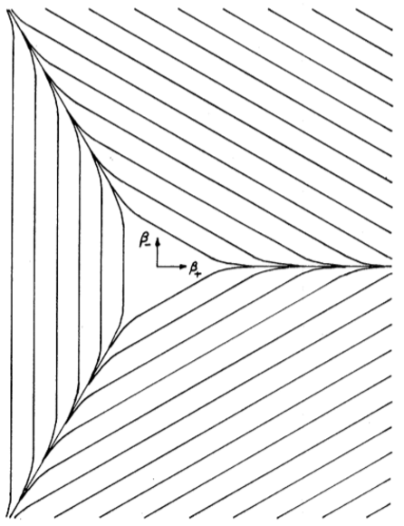
Figure 1: Equipotential lines of Bianchi IX model in $(\beta_{+},\beta_{-})$ plane [23]

By imposing that the third wall is equal to 1 we can deduce

$$-8\beta_{+}^{wall}+4\alpha=0\Longrightarrow\beta_{+}^{wall}=\frac{1}{2}\alpha,$$ (36)

where $\beta^{wall}$ defines an equipotential in the $\beta$ plane bounding the region in which the potential (space curvature) term is significant. The potential wall moves outward with the speed

$$\biggl{|}\frac{\partial\beta_{wall}}{\partial\alpha}\biggr{|}=\frac{1}{2},$$ (37)

the velocity of the point-Universe is equal to one according to (32) in free-potential region and so is doomed to impact against the wall. This means that the vacuum Bianchi IX classical evolution is constituted by an infinite series of Kasner regimes (free motions of the point-Universe), associated with continuous scatterings against the infinite potential walls[23].

We need more details on the ”bounce” and we can derive them from the ADM-Hamiltonian using the asymptotic form of the potential:

$$\mathcal{H}_{IX}=\sqrt{p_{+}^{2}+p_{-}^{2}+1/3\exp{-4\alpha-8\beta_{+}}},$$ (38)

showing that $\mathcal{H}$ is independent from $\beta_{-}$ so $p_{-}$ is a constant of motion. Another constant can be found comparing the following equation

$$\begin{split}&p_{+}^{\prime}=-\partial\mathcal{H}_{IX}/\partial\beta_{+}=+4(3\mathcal{H}_{IX})^{-1}\exp{-4\alpha-8\beta_{+}},\\ &\mathcal{H}^{{}^{\prime}}_{IX}=-\partial\mathcal{H}_{IX}/\partial\alpha=-2(3\mathcal{H}_{IX})^{-1}\exp{-4\alpha-8\beta_{+}},\end{split}$$ (39)

so we can define $k=1/2p_{+}+\mathcal{H}_{IX}=const$. These two constant of motion allow us to find the value of $\beta_{+}^{\prime}$ and $\beta_{-}^{\prime}$ after the bounce as function of their value before. Since $|\beta^{\prime}|=1$ we can parametrize $\beta_{-}^{\prime}=\sin{\theta}$ and $\beta_{+}^{\prime}=\cos{\theta}$. Using (32) and the two constant of motion we get

$$\begin{split}\mathcal{H}^{i}_{IX}\sin{\theta_{i}}=&\mathcal{H}^{f}_{IX}\sin{\theta_{f}},\\ \mathcal{H}^{i}_{IX}\bigl{(}-1/2\cos{\theta_{i}}+1\bigr{)}=&\mathcal{H}^{f}_{IX}\bigl{(}+1/2\cos{\theta_{f}}+1\bigr{)}.\end{split}$$ (40)

These can be combined to find an equation for $\theta_{f}$ as function of $\theta_{i}$,

$$\sin{\theta_{f}}-\sin{\theta_{i}}=\frac{1}{2}\sin{\left(\theta_{f}+\theta_{i}\right)},$$ (41)

which is sufficient for our purpose.

Part IV The generic cosmological problem in the Jordan Frame

The generic cosmological problem represents the Hamiltonian formalism of gravity for an inhomogeneous space. The first studies date back to the ’60s when the Landau school started to investigate the properties and the behaviour of the generic cosmological solution of the Einstein field equations.

VI Hamiltonian formulation in a general framework

Using the vierbein formalism, the 3-metric associated to a generic inhomogeneus space can be written as

$$h_{ij}(t,x^{k})=\eta_{ab}(t,x^{k})e_{i}^{a}(t,x^{k})e_{j}^{b}(t,x^{k}),$$ (42)

where $\eta_{ab}$ is its triadic representation and $a=1,2,3$ are the Lorentz indices. The corresponding line element is

$$ds^{2} =-N(t,x^{k})dt^{2}$$

$$\quad+h_{ij}(t,x^{k})\left(dx^{i}+N^{i}(t,x^{k})dt\right)\left(dx^{j}+N^{j}(t,x^{k})dt\right).$$ (43)

We can define a generic set of 3-vectors on the hypersurfaces $\varSigma_{t}^{3}$ of the ADM foliation as

$$e_{i}^{a}(t,x^{k})=O_{b}^{a}(x^{k})\partial_{i}y^{b}(t,x^{k}),$$ (44)

where $y^{b}$ denotes three scalar functions and $O_{b}^{a}$ is a $SO(3)$ matrix such that $O_{b}^{a}O_{a}^{c}=\delta_{b}^{c}$. This definition of the 3-vectors $e_{i}^{a}$ allows us to rewrite the 3-metric tensor $h_{ij}$ as

$$h_{ij}(t,x^{k}) =\underset{a}{\sum}e^{q_{a}(t,x^{k})}e_{i}^{a}(t,x^{k})e_{j}^{a}(t,x^{k})$$

$$=\underset{a}{\sum}e^{q_{a}(t,x^{k})}O_{b}^{a}(x^{k})\partial_{i}y^{b}(t,x^{k})O_{c}^{a}(x^{k})\partial_{i}y^{c}(t,x^{k}),$$ (45)

where $q_{a}(t,x^{k})=\left\{\ln{(a^{2}(t,x^{k}))},\ln{(b^{2}(t,x^{k}))},\ln{(c^{2}(t,x^{k}))}\right\}$ denotes the three inhomogeneus cosmological scale factors. Imposing the canonical transformation $\left(h_{ij},p^{ij}\right)\longrightarrow\left(q_{a},p_{a};y_{a},\pi_{a}\right)$

$$p^{ij}\partial_{t}h_{ij}=\underset{a}{\sum}p_{a}\partial_{t}q_{a}\,+\,\underset{a}{\sum}\pi_{a}\partial_{t}y_{a},$$ (46)

we obtain the superHamiltonian $\mathscr{H}_{g,JF}$ and the supermomentum $\mathscr{H}_{i,JF}^{g}$ in the new generic framework (see Appendix A for details)

$$\mathscr{H}_{g,JF} =\cfrac{2}{\sqrt{h}}\left(\cfrac{\underset{a}{\sum}p_{a}^{2}-\frac{1}{3}\left(\underset{a}{\sum}p_{a}\right)^{2}}{\phi}+\cfrac{1}{6}\phi\pi_{\phi}^{2}-\cfrac{1}{3}\underset{a}{\sum}p_{a}\pi_{\phi}\right)$$

$$+\cfrac{\sqrt{h}}{2}\left(V(\phi)-\phi\,^{3}R+2D_{i}D^{i}\phi\right),$$ (47)

$$\mathscr{H}_{i,JF}^{g}=\pi_{\phi}\partial_{i}\phi+\pi_{a}\partial_{i}y^{a}+p_{a}\partial_{i}q^{a}+2p_{a}\left(O^{-1}\right)_{a}^{b}\partial_{i}O_{b}^{a}.$$ (48)

VII The generic cosmological problem in Misner-like variables

Let us introduce the Misner-like variables $\left\{\alpha(t,x^{k}),\beta_{+}(t,x^{k}),\beta_{-}(t,x^{k})\right\}$ via the transformation

$$\Biggl{\{}\begin{array}[]{l}q_{1}(t,x^{k})=\left(\alpha(t,x^{k})+\beta_{+}(t,x^{k})+\sqrt{3}\beta_{-}(t,x^{k})\right)\\ q_{2}(t,x^{k})=\left(\alpha(t,x^{k})+\beta_{+}(t,x^{k})-\sqrt{3}\beta_{-}(t,x^{k})\right)\\ q_{3}(t,x^{k})=\left(\alpha(t,x^{k})-2\beta_{+}(t,x^{k})\right)\end{array}$$ (49)

Imposing the canonical condition $\left(q_{a},p_{a}\right)\longrightarrow\left(\alpha,p_{\alpha};\beta_{+},p_{+};\beta_{-},p_{-}\right)$

$$p_{\alpha}\dot{\alpha}+p_{+}\dot{\beta}_{+}+p_{-}\dot{\beta}_{-}=\underset{a}{\sum}p_{a}\partial_{t}q_{a},$$ (50)

we can rewrite the $f(R)$ superHamiltonian (47) of the generic cosmological problem in Misner-like variables

$$\begin{split}\mathscr{H}&{}_{g,JF}=\\ &\cfrac{2e^{-\frac{3}{2}\alpha}}{\mathbf{v}}\left[\cfrac{1}{6\phi}\left(p_{+}^{2}+p_{-}^{2}\right)+\cfrac{1}{6}\pi_{\phi}^{2}\phi-\cfrac{1}{3}p_{\alpha}\pi_{\phi}+U\left(\alpha,\beta_{\pm},\phi\right)\right],\end{split}$$ (51)

where $\textbf{v}(x^{l})$ = $\det\left(e_{i}^{a}\right)$ and $U\left(\alpha,\beta_{\pm},\phi\right)=\cfrac{\mathbf{v}^{2}}{4}e^{3\alpha}\left(V(\phi)-\phi\,^{3}R+2D_{i}D^{i}\phi\right)$.

It is clear that, differently from the case in General Relativity [3] where the superHamiltonian takes the form

$$\mathcal{H}_{g}=\cfrac{2e^{-\frac{3}{2}\alpha}}{\mathbf{v}}\left(-p_{\alpha}^{2}+p_{+}^{2}+p_{-}^{2}+U(\alpha,\beta_{\pm})\right),$$ (52)

in the case of the $f(R)$ theories in the Jordan frame we lose the the pseudo-Riemannian structure. It is also evident that the equation (51) is the classical counterpart in the cosmological context of the Wheeler-De Witt quantum-gravitational equation (24). Therefore, the same considerations about the problem of identifying a time variable apply. As we have already done, we highlight the linearity of the equation with respect to the conjugated momentum $p_{\alpha}$ and, therefore, the formal analogy between the equation (51) and a Schrodinger-like equation, once one assigns to $\alpha$ the role of the timelike variable of the theory. The presence of a potential term still does not allow to construct a Hilbert space for physical quantum states.

Part V Classical $f(R)$ Cosmology

When we use the term classical cosmology we refer to the description of the Universe using the tools provided by General Relativity and, in this case, the equivalence with Brans-Dicke theory of $f(R)$ models. Our purpose is to analyse the Bianchi IX model, which is the prototype of the generic cosmological solution, in Jordan frame and try to solve some already known issues of this model in GR, such as its chaotic behaviour as we are going through the cosmological singularity. In order to achieve this result we need to follow some intermediate steps: find a solution for the Bianchi I model, i.e. the Kasner solution, and use these solutions to discuss some properties of the potential terms. We want to define a class of $f(R)$ theory for which we can neglect the term $V(\phi)$ in a way that the solutions became independent from the specific functional form of the theory. Then we discuss the properties of the potential term of the Bianchi IX model and try to find a region, in the space of parameters that describes the Kasner solutions, which removes the chaos. Finally, we will discuss the properties of our cosmological model, studying the dynamical features of the bounces that characterize the Bianchi IX model.

VIII Kasner solution for the Bianchi I model

The Bianchi I Universe corresponds to the case $V_{B}\left(\alpha,\beta_{\pm},\phi\right)=0$, since the structure constants of the isometry group are all zero. Strictly speaking, we are assuming also the potential $V\left(\phi\right)$ to be negligible. The conditions under which the potential of the $f(R)$ theory is negligible will be discussed later. The superHamiltonian (51) becomes

$$\mathcal{H}_{BI,JF}=\cfrac{2e^{-\frac{3}{2}\alpha}}{\mathbf{v}}\left[\cfrac{1}{6\phi}\left(p_{+}^{2}+p_{-}^{2}\right)+\cfrac{1}{6}\pi_{\phi}^{2}\phi-\cfrac{1}{3}p_{\alpha}\pi_{\phi}\right].$$ (53)

In the framework of Bianchi models, the anisotropies of the Universe $\beta_{\pm}$ represent the 2 physical degrees of freedom of Einstenian gravity, the variable $\alpha$ represents an embedding degree of freedom and the variable $\phi$ is a massive mode. Solving classically the superHamiltonian constraint (53) with respect to the conjugate momentum $\pi_{\phi}$, we get the following quadratic equation

$$\pi_{\phi}^{2}-\cfrac{2p_{\alpha}}{\phi}\pi_{\phi}+\cfrac{\left(p_{+}^{2}+p_{-}^{2}\right)}{\phi^{2}}=0,$$ (54)

which admits the solutions

$$\pi_{\phi\,_{1,2}}=\cfrac{p_{\alpha}}{\phi}\pm\cfrac{1}{\phi}\sqrt{p_{\alpha}^{2}-p_{+}^{2}-p_{-}^{2}}=-h_{\phi\,_{1,2}}.$$ (55)

The next step in the procedure consists in the imposition of the so-called time gauge which sets the lapse function $N$

$$\dot{\phi}=N\cfrac{\partial\mathcal{H}_{BM\,\mathrm{I},JF}}{\partial\pi_{\phi}}=\cfrac{2Ne^{-\frac{3}{2}\alpha}}{3\mathbf{v}}\left(\phi\pi_{\phi}-p_{\alpha}\right)=1,$$ (56)

$$N=N_{ADM}=\cfrac{3\mathbf{v}e^{\frac{3}{2}\alpha}}{2\left(\phi\pi_{\phi}-p_{\alpha}\right)}.$$ (57)

Since $N$ is always positive, we obtain the condition $\phi\pi_{\phi}>p_{\alpha}$ which constraints the choice of the positive sign in equation (55). From the Hamilton’s equations

$$\left\{\begin{array}[]{l}\cfrac{\partial\alpha}{\partial\phi}=\cfrac{\partial h_{\phi}}{\partial p_{\alpha}}=-\cfrac{1}{\phi}\left(1+\cfrac{p_{\alpha}}{\sqrt{p_{\alpha}^{2}-p_{+}^{2}-p_{-}^{2}}}\right)\\ \cfrac{\partial p_{\alpha}}{\partial\phi}=-\cfrac{\partial h_{\phi}}{\partial\alpha}=0\end{array}\right.$$ (58)

we can derive the equation of motion

$$\alpha\left(\phi\right)=-Kln\left(\phi\right)+\alpha_{0},$$ (59)

where we set $\alpha_{0}=0$ by choosing the initial condition $\alpha(0)=0$ and where $K$ is a constant of motion defined as

$$K=1+\cfrac{p_{\alpha}}{\sqrt{p_{\alpha}^{2}-p_{+}^{2}-p_{-}^{2}}}.$$ (60)

Since the Misner variable $\alpha$ is related to the volume of the Universe, the constant $K$ must always be real. Consequently, we must impose the relation

$$p_{\alpha}^{2}>p_{+}^{2}+p_{-}^{2},$$ (61)

which constraints the value of $|K|>1$. The Hamilton’s equations takes the following form: $d\beta_{\pm}/d\phi=\partial h_{\phi}/\partial p_{\pm}$ and, since the Hamiltonian does not depend on the coordinates, the momenta are constant. We can express the Misner coordinates as function of the scalar field:

$$\begin{split}&\alpha=-\left(1+\frac{p_{\alpha}}{\sqrt{p_{\alpha}^{2}-p_{+}^{2}-p_{-}^{2}}}\right)ln{\phi},\\ &\beta_{\pm}=-\left(\frac{p_{\pm}}{\sqrt{p_{\alpha}^{2}-p_{+}^{2}-p_{-}^{2}}}\right)ln{\phi}.\end{split}$$ (62)

By dividing between $\beta_{\pm}\left(\phi\right)$ and $\alpha\left(\phi\right)$ we can find $\beta_{\pm}=\beta_{\pm}\left(\alpha\right)$

$$\beta_{\pm}\left(\alpha\right)=\frac{p_{\pm}}{p_{\alpha}\pm\sqrt{p_{\alpha}^{2}-p_{+}^{2}-p_{-}^{2}}}\cdot\alpha.$$ (63)

IX Potential term of $f(R)$ theory

We want to deal with the most general solution, so we have to set some constraint on the functional form of the theory. As the model we are analysing is important only in a pre-inflation scenario , we are interested in the limit $\alpha\rightarrow-\infty$ and so we want that the potential term of $\phi$ in the Hamiltonian of the system vanish as we are going to the cosmological singularity. So we can work with a class of theories, that obeys to this constraint, instead of dealing with a specific theory with a specific functional form of the potential. In order to achieve our goal we will use the kasner solutions found in the previous section and then we will discuss the functional form with the dominant diverging term which admits the limit we are looking for. Finally, we will define a concrete constraint of the functional form of the potential of the $f(R)$ theory.

We have to rewrite the kasner solutions because we are interested in $\phi$ as a function of $\alpha$. The Kasner solution gives us $\alpha(\phi)$ in eq.(62) that can be easily inverted to find $\phi(\alpha)$

$$\alpha=-\left(1+\frac{p_{\alpha}}{\sqrt{p_{\alpha}^{2}-p_{+}^{2}-p_{-}^{2}}}\right)ln{\phi},$$ (64)

and

$$\phi=e^{-\frac{\alpha}{K}},$$ (65)

whit $K=1+p_{\alpha}/\sqrt{p_{\alpha}^{2}-p_{+}^{2}-p_{-}^{2}}$. We can assume that $V(\phi)\propto\phi^{n}$, because other dependence are forbidden by the condition chosen on the potential.

$$e^{3\alpha}V(\phi)\propto e^{3\alpha}e^{-n\alpha/K}=e^{\left(3-n/K\right)\alpha},$$ (66)

we have to study the sign of $3-n/K$ because it must be positive in order to have a vanishing potential. We will now calculate the maximum $n$ that respects the condition

$$3-n/K=3-\frac{n}{1+\frac{p_{\alpha}}{\sqrt{p_{\alpha}^{2}-p_{+}^{2}-p_{-}^{2}}}}>0.$$ (67)

The inequalities can be rewritten by solving it for $n$

$$n<3\left(1+\frac{p_{\alpha}}{\sqrt{p_{\alpha}^{2}-p_{+}^{2}-p_{-}^{2}}}\right).$$ (68)

The function of the momenta is strictly increasing and its maximum and minimum value are defined by its limits, respectively to $-\infty$ and to $+\infty$.

$$-1<\frac{p_{\alpha}}{\sqrt{p_{\alpha}^{2}-p_{+}^{2}-p_{-}^{2}}}<1,$$ (69)

and so the value of $K$ is also limited between 0 and 2. We are interested to the maximum value of $n$ and then we get $K=2$, which gives us the value of $n$ we are looking for

$$n_{MAX}=6.$$ (70)

For all the metric $f(R)$ theories, with a potential term which diverges slower than $\phi^{6}$, the present and following analyses hold.

The form of the function $f$, due to a polynomial form of the potential $V(\phi)$, can be derived using the following differential equation:

$$f^{\prime\prime}(R)[R-V^{\prime}(f^{\prime}(R))]=0.$$ (71)

The first solution ($f(R)=R$) leads to the General Relativity, while the second solution gives us the following form of the function:

$$f(R)=(n-1)\biggl{(}\frac{R}{n}\biggr{)}^{\frac{n}{n-1}}.$$ (72)

so we can fix $n\in(1,6]$.

X Chaotic behaviour of the Bianchi IX potential

We have already seen that the dynamics of the Bianchi IX model is completely determined by the potential. The form of the potential, in its asymptotic form, is a wall with a triangular symmetry but in a $f(R)$ theory it is multiplied by the scalar field $\phi$. This feature gives us the chance to remove the chaotic behaviour of this model, characterized by oscillations from one Kasner solution to another. We are looking for a region, in the space of the parameters that characterized the Kasner solutions, that ensures us that the potential term will vanish as we are going to the cosmological singularity. We analyse the role of the scalar field using the method of consistent potential (MCP), i.e. we assume that the approach to the singularity is asymptotically velocity term dominated[24]. If this is true, the model approaches closely to a Kasner solution. The superHamiltonian constraint takes the form

$$\mathcal{H}_{IX,JF}=\mathcal{H}_{k}+\mathcal{H}_{v},$$ (73)

where $\mathcal{H}_{k}$ is the kinetic term and $\mathcal{H}_{v}$ stands as

$$\begin{split}2&\mathcal{H}_{v}=\phi\biggl{\{}\left(e^{2\alpha+2\beta_{+}+2\sqrt{3}\beta_{-}}+e^{2\alpha+2\beta_{+}-2\sqrt{3}\beta_{-}}+e^{2\alpha-4\beta_{+}}\right)\\ &-2\left(e^{2\alpha+2\beta_{+}}+e^{2\alpha-\beta_{+}+\sqrt{3}\beta_{-}}+e^{2\alpha-\beta_{+}-\sqrt{3}\beta_{-}}\right)\biggr{\}}+e^{3\alpha}V(\phi).\end{split}$$ (74)

In these variables, the singularity occurs as $\alpha\rightarrow-\infty$, and as we have discussed in the previous section $e^{3\alpha}V(\phi)\rightarrow 0$ going to the singularity, so we shall ignore this term. The method of consistent potential (MCP) will be used in order to define a Kasner stability region in which the characteristic oscillation of the Mixmaster Universe are suppressed after a given sequence. The MCP requires to assume $\mathcal{H}=\mathcal{H}_{k}$. Variation of this Hamiltonian yields equations with the solution obtained in eq.(62) which we are going to express as function of $\alpha$

$$\begin{split}&\beta_{\pm}=\beta_{\pm}^{{}^{\prime}}\alpha,\\ &\phi=e^{-\frac{\alpha}{K}},\end{split}$$ (75)

where $K$ and $v_{\pm}$ are defined as

$$\begin{split}&\beta{{}^{\prime}}_{\pm}=\frac{p_{\pm}}{\sqrt{p_{\alpha}^{2}-p_{+}^{2}-p_{-}^{2}}},\\ &\text{$K$}=\left(1+\frac{p_{\alpha}}{\sqrt{p_{\alpha}^{2}-p_{+}^{2}-p_{-}^{2}}}\right).\end{split}$$ (76)

The minisuperspace potential is dominated by the first three terms of r.h.s. of eq. (74)

$$2\mathcal{H}_{v}\approx\phi\left(e^{2\alpha+2\beta_{+}+2\sqrt{3}\beta_{-}}+e^{2\alpha+2\beta_{+}-2\sqrt{3}\beta_{-}}+e^{2\alpha-4\beta_{+}}\right),$$ (77)

so we can write $K$ as a function of $\beta^{\prime}_{+}$ and $\beta^{\prime}_{-}$ considering that

$$\beta{{}^{\prime}}_{+}^{2}+\beta{{}^{\prime}}_{-}^{2}=\frac{p_{+}^{2}+p_{-}^{2}}{\left(p_{\alpha}+\sqrt{p_{\alpha}^{2}-p_{+}^{2}-p_{-}^{2}}\right)^{2}},$$

and we can invert this relation to find $p_{+}^{2}+p_{-}^{2}$

$$p_{+}^{2}+p_{-}^{2}=\frac{4p_{\alpha}^{2}\left(\beta{{}^{\prime}}_{+}^{2}+\beta{{}^{\prime}}_{-}^{2}\right)}{\left(\beta{{}^{\prime}}_{+}^{2}+\beta{{}^{\prime}}_{-}^{2}-1\right)^{2}},$$ (78)

inserting eq. (78) into the definition of $K$ we can express it as function of $\beta_{+}$ and $\beta_{-}$:

$$\frac{1}{2K}=\frac{\beta{{}^{\prime}}_{+}^{2}+\beta{{}^{\prime}}_{-}^{2}-1}{4\beta{{}^{\prime}}_{+}^{2}+4\beta{{}^{\prime}}_{-}^{2}}.$$ (79)

Substitution of (76) and (79) into (77), yields to

$$\begin{split}2\mathcal{H}_{v}\approx&\exp\biggl{\{}{2\alpha\left(1+\beta{{}^{\prime}}_{+}+\sqrt{3}\beta{{}^{\prime}}_{-}-\frac{\beta{{}^{\prime}}_{+}^{2}+\beta{{}^{\prime}}_{-}^{2}-1}{4\beta{{}^{\prime}}_{+}^{2}+4\beta{{}^{\prime}}_{-}^{2}}\right)}\biggr{\}}\\ +&\exp\biggl{\{}{2\alpha\left(1+\beta{{}^{\prime}}_{+}-\sqrt{3}\beta{{}^{\prime}}_{-}-\frac{\beta{{}^{\prime}}_{+}^{2}+\beta{{}^{\prime}}_{-}^{2}-1}{4\beta{{}^{\prime}}_{+}^{2}+4\beta{{}^{\prime}}_{-}^{2}}\right)}\biggr{\}}\\ +&\exp\biggl{\{}{2\alpha\left(1-2\beta{{}^{\prime}}_{+}-\frac{\beta{{}^{\prime}}_{+}^{2}+\beta{{}^{\prime}}_{-}^{2}-1}{4\beta{{}^{\prime}}_{+}^{2}+4v_{-}^{2}}\right)}\biggr{\}}.\end{split}$$ (80)

We are looking for some values of $\beta_{+}$ and $\beta_{-}$ which make all the terms going to zero as $\alpha\rightarrow-\infty$. In order to achieve our purpose we had to solve, at the same time, all these inequalities:

$$\begin{split}&1+\beta{{}^{\prime}}_{+}+\sqrt{3}\beta{{}^{\prime}}_{-}-\frac{\beta{{}^{\prime}}_{+}^{2}+\beta{{}^{\prime}}_{-}^{2}-1}{4\beta{{}^{\prime}}_{+}^{2}+4\beta{{}^{\prime}}_{-}^{2}}>0,\\ &1+\beta{{}^{\prime}}_{+}-\sqrt{3}\beta{{}^{\prime}}_{-}-\frac{\beta{{}^{\prime}}_{+}^{2}+\beta{{}^{\prime}}_{-}^{2}-1}{4\beta{{}^{\prime}}_{+}^{2}+4\beta{{}^{\prime}}_{-}^{2}}>0,\\ &1-2\beta{{}^{\prime}}_{+}-\frac{\beta{{}^{\prime}}_{+}^{2}+\beta{{}^{\prime}}_{-}^{2}-1}{4\beta{{}^{\prime}}_{+}^{2}+4\beta{{}^{\prime}}_{-}^{2}}>0.\end{split}$$ (81)

With the help of the software Mathematica we have solved the three inequalities to find the values of $\beta_{+}$ and $\beta_{-}$ which can make all the three exponential to vanish at the same time. The explicit form of the Kasner stability region can be found in Appendix B, now we just want to show its graph.

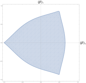
Figure 2: Kasner stability region as function of $\beta^{\prime}_{+}$ and $\beta^{\prime}_{-}$

Now our purpose is to characterize the dynamical features of the ”bounces” typical of the the Bianchi IX model. We want to check if the Kasner stability region is an attractor for the Mixmaster dynamics. First of all, we shall remember that, near the singularity, the matter and radiation density terms are negligible because the dynamics of the Universe is dominated by the curvature term due to the geometry of the space-time. The potential term of the Bianchi IX cosmology depends on the variable $\alpha$ and this feature complicates the dynamics with respect to the Kasner solution, generating in principle a chaotic evolution. The vacuum Bianchi IX dynamics is constituted by an infinite series of Kasner regimes, associated with the continuous scatterings against the infinite potential walls. The purpose of this chapter is to verify if, thanks to the additional degree of freedom introduced by the choice of $f(R)$ framework, we are led to remove the chaotic behaviour. We have already find a region, in the space of the parameters $(\beta_{+},\beta_{-})$ that describe the Kasner solutions, for which the point-Universe does not impact against the potential walls. Now we want to verify if the natural evolution of the system, starting from any point in the parameters space, will bring the point-Universe to the Kasner stability region. The calculus of the equation of motion is very complicated because of the potential term, so we will not integrate numerically the equation of motion (which are not clearly analytical integrable) to determinate the evolution of the cosmological model. Instead, recalling the method used to find the eq.(41) we will search for three constants of motion that allow us to find the new Kasner solution, after the bounce, as a function of the previous solution. The superHamiltonian constraint takes the form:

$$\mathcal{H}_{IX,JF}=\phi\pi_{\phi}^{2}-2\pi_{\phi}p_{\alpha}+\frac{p_{+}^{2}+p_{-}^{2}}{\phi}+\phi e^{3\alpha}V_{IX}(\alpha,\beta_{\pm})=0.$$ (82)

Where the potential of the model is

$$\begin{split}V_{IX}(\alpha,&\beta_{\pm})=\\ &\frac{1}{2}e^{-3\alpha}\biggl{\{}\left(e^{2\alpha+2\beta_{+}+2\sqrt{3}\beta_{-}}+e^{2\alpha+2\beta_{+}-2\sqrt{3}\beta_{-}}+e^{2\alpha-4\beta_{+}}\right)\\ &-\left(e^{2\alpha+2\beta_{+}}+e^{2\alpha-\beta_{+}+\sqrt{3}\beta_{-}}+e^{2\alpha-\beta_{+}-\sqrt{3}\beta_{-}}\right)\biggr{\}},\end{split}$$ (83)

where the first three terms dominate as we are going to the singularity. The potential $V(\phi)$ can be neglected, as we saw previously. We will solve the superHamiltonian constraint with respect to the appropriate time-like variable $\phi$:

$$\pi_{\phi}=-h_{\phi}=\frac{1}{\phi}\left\{p_{\alpha}+\sqrt{p_{\alpha}^{2}+p_{+}^{2}+p_{-}^{2}-6\phi e^{3\alpha}V_{IX}(\alpha,\beta_{\pm})}\right\}.$$ (84)

In the standard case, the evolution of the Universe is described by giving $\beta_{\pm}$ as functions of the scalar field $\phi$. The entire problem is governed by the function $V_{IX}(\alpha,\beta_{\pm})$, which has the symmetry of an equilateral triangle as in FIG.1. For $\beta_{+}\rightarrow-\infty$ it gets the following asymptotic form

$$V_{IX}\sim\frac{1}{3}e^{2\alpha-4\beta_{+}}$$ (85)

showing one of the three exponentially steep walls on which the equipotentials are straight lines. The corners of this triangular potential are open; it satisfies the condition $V_{IX}\geq 0$ and vanishes only at the origin, where $V_{IX}\approx 2\left(\beta_{+}^{2}+\beta_{-}^{2}\right)$. Because the potential rises so steeply for large $\beta$, little time is spent with the $\beta$ bouncing against the potential wall and most of the time is spent in free motion when $V_{IX}$ can be neglected, so the motion is described by a Kasner solution:

$$\begin{split}&\alpha=-\left(1+\frac{p_{\alpha}}{\sqrt{p_{\alpha}^{2}-p_{+}^{2}-p_{-}^{2}}}\right)ln{\phi},\\ &\beta_{\pm}=\left(\frac{p_{\pm}}{\sqrt{p_{\alpha}^{2}-p_{+}^{2}-p_{-}^{2}}}\right)ln{\phi}.\end{split}$$ (86)

By defining the velocities as the derivatives with respect to the logarithm of scalar field

$$\begin{split}&\alpha^{\prime}=1+\frac{p_{\alpha}}{\sqrt{p_{\alpha}^{2}-p_{+}^{2}-p_{-}^{2}}},\\ &v_{\pm}=\frac{p_{\pm}}{\sqrt{p_{\alpha}^{2}-p_{+}^{2}-p_{-}^{2}}},\end{split}$$ (87)

with the condition $(\alpha^{\prime}-1)^{2}-(\beta_{+}^{\prime})^{2}-(\beta_{-}^{\prime})^{2}=1$. For the sake of simplicity we study the bouncing against the potential of an assigned Kasner solution, considering the vertical wall which intersects the axes $\beta_{+}$. We recall that the choice of this wall is equivalent to anyother one, due to the traingular simmetry of the potential (under a rotation of $\frac{\pi}{3}$). We use the asymptotic form of the superHamiltonian using eq.(85)

$$\mathcal{H}_{IX,JF}=\frac{1}{\phi}\left\{p_{\alpha}+\sqrt{p_{\alpha}^{2}-p_{+}^{2}-p_{-}^{2}+\frac{1}{3}e^{+2\alpha-4\beta_{+}}}\right\}.$$ (88)

It is independent of $\beta_{-}$ in this approximation, so $p_{-}$ will be constant during the bounce. Another constant of motion can be found by comparing these equations

$$\begin{split}&p_{+}^{\prime}=-\frac{\partial\mathcal{H}_{IX,JF}}{\partial\beta_{+}}=4\mathcal{H}_{IX,JF}^{-1}e^{2\alpha-4\beta_{+}},\\ &p_{\alpha}^{\prime}=-\frac{\partial\mathcal{H}_{IX,JF}}{\partial\alpha}=-2\mathcal{H}_{IX,JF}^{-1}e^{2\alpha-4\beta_{+}},\end{split}$$ (89)

with the results that $\frac{1}{2}p_{+}+p_{\alpha}=const$. A third constant of motion can be found in the same way, by comparing the two terms $\frac{\partial\phi\pi_{\phi}}{\partial\phi}$ and $\frac{\partial p_{\alpha}}{\partial\phi}$ , so we have $\phi\pi_{\phi}-1/2p_{\alpha}=const$. Thus, the system of equations that we want to solve is:

$$\left\{\begin{array}[]{l}1/2p_{\alpha}^{{}^{\prime}}+\sqrt{p_{\alpha}^{2^{\prime}}-p_{+}^{2^{\prime}}-p_{-}^{2^{\prime}}}=1/2p_{\alpha}+\sqrt{p_{\alpha}^{2}-p_{+}^{2}-p_{-}^{2}},\\ \frac{1}{2}p_{+}^{{}^{\prime}}+p_{\alpha}^{{}^{\prime}}=\frac{1}{2}p_{+}+p_{\alpha},\\ p_{-}^{{}^{\prime}}=p_{-},\end{array}\right.$$ (90)

where the primate quantities are the ones after the bounce. In order to solve the system we use the Kasner solution to write the equations as functions of $v_{\pm},v_{\alpha}$. The velocities satisfy the condition: $v_{\alpha}^{2}-v_{+}^{2}-v_{-}^{2}=1$, which suggest the following change of variables:

$$\begin{split}&v_{\alpha}=\cosh{\varphi},\\ &v_{+}=\sinh{\varphi}\cos{\theta},\\ &v_{-}=\sinh{\varphi}\sin{\theta}.\end{split}$$ (91)

Far from the potential walls, the Hamiltonian is independent from the coordinates and so the conjugate momenta are constants. We can rewrite the constant of motion as function of $\varphi$ and $\theta$:

$$\left\{\begin{array}[]{l}\mathcal{H}_{IX,JF}\left(\frac{1}{2}\cosh{\varphi}+1\right),\\ \mathcal{H}_{IX,JF}\left(\frac{1}{2}\sinh{\varphi}\cos{\theta}+\cosh{\varphi}\right),\\ \mathcal{H}_{IX,JF}\sinh{\varphi}\sin{\theta}.\end{array}\right\}$$ (92)

We have developed a software to help us to simulate the evolution of the system. We have performed many simulations to understand if the system was able to reach the stability region starting from any point in the space of the parameters that describes the Kasner solutions $(\beta_{+}^{{}^{\prime}},\beta_{-}^{{}^{\prime}})$. Since $|\beta_{\pm}^{{}^{\prime}}|<1$ we choose to evolve 10.000 models inside 4 circles on the four corners of the square with a radius $1/10$.

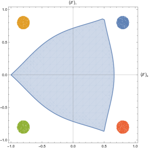
(a)

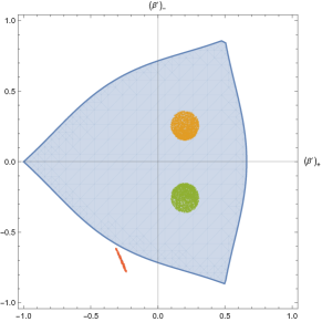
(b)

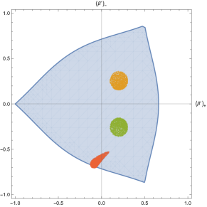
(c)

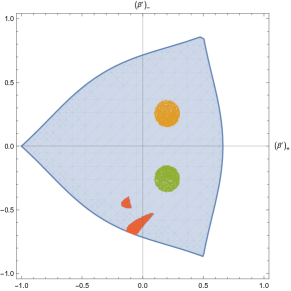
(d)

Figure 3: The evolution of $10^{4}$ models through the map, after three bounces all the solutions has reached the stability region.

The constants of motion are written as functions of $v_{+}$ and $v_{-}$ while the Kasner stability region is a function of $\beta_{\pm}^{{}^{\prime}}$, we can write $\beta_{\pm}^{{}^{\prime}}=\frac{v_{\pm}}{v_{\alpha}+1}$ and evaluate the position of the model in the Kasner parameter’ space after every bounce against the potential walls. Every run of the model, started with random parameters inside the circles, has reached the stability region and so we can deduce that the natural evolution of a Bianchi IX cosmology in the Jordan frame naturally removes chaos.

Part VI Quantum $f(R)$ Cosmology

With the term quantum cosmology (QC) we refer to the application of the quantum theory of gravity to the entire Universe. The existence of such a theory would clarify the physics of the Big Bang, describing the entire Universe like a relativistic-quantum object.

XI Bianchi I Universe

By promoting the superHamiltonian constraint (53) to a quantum operator annihilating the wave function $\varphi\left(\alpha,\beta_{\pm},\phi\right)$, we obtain the Wheeler-De Witt equation

$$\begin{array}[]{l}\mathcal{\hat{H}}_{B\,\mathrm{I},JF}|\varphi\rangle\\ =\cfrac{2e^{-\frac{3}{2}\alpha}}{\mathbf{v}}\left[\cfrac{1}{6\phi}\left(\hat{p}_{+}^{2}+\hat{p}_{-}^{2}\right)+\cfrac{1}{6}\hat{\pi}_{\phi}^{2}\phi-\cfrac{1}{3}\hat{p}_{\alpha}\hat{\pi}_{\phi}\right]|\varphi\rangle\\ =\cfrac{2e^{-\frac{3}{2}\alpha}}{\mathbf{v}}\hbar^{2}\left[\cfrac{1}{3}\partial_{\alpha}\partial_{\phi}-\cfrac{1}{6\phi}\left(\partial_{+}^{2}+\partial_{-}^{2}\right)-\cfrac{\phi}{6}\partial_{\phi}^{2}\right]\varphi=0.\end{array}$$ (93)

In the kinetic term mixed impulses in the variables $\left(\alpha,\phi\right)$ appear and consequently, it is impossible to trace the formalism back to the problem of a free relativistic particle. In the following, we will assume $\phi$ as a timelike variable. Such a choice, in the Jordan frame, is interesting for the idea of using a gravitational degree of freedom as a quantum time. In this way, the problem of time in quantum gravity could be addressed through a generalization of General Relativity. We choose a particular factor ordering of the Wheeler-De Witt equation rewriting the equation as

$$\cfrac{2e^{-\frac{3}{2}\alpha}}{\mathbf{v}}\hbar^{2}\left[\cfrac{1}{3}\partial_{\alpha}\partial_{\phi}-\cfrac{1}{6\phi}\left(\partial_{+}^{2}+\partial_{-}^{2}\right)-\cfrac{1}{6}\partial_{\phi}\left(\phi\partial_{\phi}\right)\right]\varphi=0.$$ (94)

Substituting in eq.(94) the natural solution

$$\varphi\left(\alpha,\beta_{\pm},\phi\right)=Ae^{i\left(k_{+}\beta_{+}+k_{-}\beta_{-}+k_{\alpha}\alpha\right)}f(\phi),$$ (95)

we obtain a Bessel differential equation for the function $f\left(\phi\right)$

$$\phi^{2}\cfrac{\partial^{2}f}{\partial\phi^{2}}+\phi\cfrac{\partial f}{\partial\phi}\left(1-2ik_{\alpha}\right)-\left(k_{+}^{2}+k_{-}^{2}\right)f=0,$$ (96)

with solution

$$f(\phi)=c_{1}\phi^{i\left(k_{\alpha}-\sqrt{k_{\alpha}^{2}-k_{+}^{2}-k_{-}^{2}}\right)}\left(c_{2}+\phi^{2i\sqrt{k_{\alpha}^{2}-k_{+}^{2}-k_{-}^{2}}}\right),$$ (97)

where $(c_{1},c_{2})$ are arbitrary constants to be fixed by the initial conditions. One can easily note that, by choosing the variable $\phi$ as the internal time of the theory, the frequency separation procedure is unfeasible due to the lack of the term $e^{ik_{\phi}\phi}$. Since the WDW equation (94) is linear, the superposition principle holds , so the general solution, describing the quantum dynamics of the Bianchi I Universe, admits the following Fourier representation

$$\Phi\left(\alpha,\beta_{\pm},\phi\right)=\int_{-\infty}^{+\infty}\int_{-\infty}^{+\infty}dk_{\alpha}dk_{+}dk_{-}A\left(k_{\alpha},k_{\pm}\right)\varphi\left(\alpha,\beta_{\pm},\phi\right),$$ (98)

where we choose

$$\begin{array}[]{l}A\left(k_{\alpha},k_{\pm}\right)\\ =\cfrac{1}{\sqrt{\left(2\pi\right)^{3}}\sigma_{\alpha}\sigma_{+}\sigma_{-}}\;e^{-\left(\frac{\left(k_{\alpha}-\bar{k}_{\alpha}\right)^{2}}{2\sigma_{\alpha}^{2}}+\frac{\left(k_{+}-\bar{k}_{+}\right)^{2}}{2\sigma_{+}^{2}}+\frac{\left(k_{-}-\bar{k}_{-}\right)^{2}}{2\sigma_{-}^{2}}\right)},\end{array}$$ (99)

as a Gaussian probability distribution, assuming we start at the initial time $\phi_{0}$ with a Gaussian wave packet.

XI.1 The probability density

In order to define a Hilbert space, we must introduce a positive-defined scalar product and, therefore, a positive-defined probability that is preserved over time. We can build the scalar product induced by the Wheeler-De Witt equation (94) by imposing the relation

$$\varphi^{*}\eqref{11.2}-\varphi\eqref{11.2}^{*}=0,$$ (100)

where $\varphi^{*}$ is the complex conjugate wave function and $\eqref{11.2}^{*}$ represents the complex conjugate Wheeler-De Witt equation. In particular, the relation (100) explicitates as

$$\begin{array}[]{l}\cfrac{1}{6\phi}\left(\varphi^{*}\partial_{+}^{2}\varphi-\varphi\partial_{+}^{2}\varphi^{*}+\varphi^{*}\partial_{-}^{2}\varphi-\varphi\partial_{-}^{2}\varphi^{*}\right)+\\ +\cfrac{1}{6}\left(\varphi^{*}\partial_{\phi}\left(\phi\partial_{\phi}\varphi\right)-\varphi\partial_{\phi}\left(\phi\partial_{\phi}\varphi^{*}\right)\right)+\\ -\cfrac{1}{3}\left(\varphi^{*}\partial_{\alpha}\partial_{\phi}\varphi-\varphi\partial_{\alpha}\partial_{\phi}\varphi^{*}\right)=0.\end{array}$$ (101)

In order to search for a probability density, we want to reconduce the quantity (101) to a continuity equation

$$\begin{array}[]{ccc}\partial_{\mu}J^{\mu}=0,&&\mu=\left(\alpha,\beta_{+},\beta_{-},\phi\right)\end{array},$$ (102)

We emphasize that we have relaxed the request to use a covariant four-divergence, in favor of a Minkowskian one. Considering the so-called minisupermetric $g^{\mu\nu}$ in the equation (94)

$$g^{\mu\nu}=\left(\begin{array}[]{cccc}0&0&0&-\frac{1}{6}\\ 0&\frac{1}{6\phi}&0&0\\ 0&0&\frac{1}{6\phi}&0\\ -\frac{1}{6}&0&0&\frac{\phi}{6}\end{array}\right)$$ (103)

we can explicitate the relation (102) as

$$\begin{array}[]{l}\partial_{\mu}J^{\mu}=\\ \cfrac{1}{6\phi}\left(\partial_{+}J_{+}+\partial_{-}J_{-}\right)+\cfrac{1}{6}J_{\phi}\\ +\cfrac{\phi}{6}\partial_{\phi}J_{\phi}-\cfrac{1}{6}\partial_{\alpha}J_{\phi}-\cfrac{1}{6}\partial_{\phi}J_{\alpha}.\end{array}$$ (104)

By comparing equations (101) and (104), the components of the conserved four-current $J^{\mu}$ take the form

$$\left\{\begin{array}[]{c}J_{\pm}=\left(\varphi^{*}\partial_{\pm}\varphi-\varphi\partial_{\pm}\varphi^{*}\right)\\ J_{\phi}=\left(\varphi^{*}\partial_{\phi}\varphi-\varphi\partial_{\phi}\varphi^{*}\right)\\ J_{\alpha}=\left(\varphi^{*}\partial_{\alpha}\varphi-\varphi\partial_{\alpha}\varphi^{*}\right)\end{array}\right.$$ (105)

and, in analogy with the Klein-Gordon theory, the quantity

$$\int_{V_{\infty}}iJ_{\phi}d\beta_{\pm}d\alpha=\langle\varphi|\varphi\rangle,$$ (106)

turns out to be a good candidate for a probabilty. However, this scalar product is not positive-defined and, unlike the case of the Klein-Gordon theory, the separation of frequencies cannot be performed. We now define the probability density

$$\begin{array}[]{cl}\rho_{\phi}&=i\left(\varphi^{*}\partial_{\phi}\varphi-\varphi\partial_{\phi}\varphi^{*}\right)\\ &=i\left(f^{*}\partial_{\phi}f-f\partial_{\phi}f^{*}\right).\end{array}$$ (107)

Considering the function $f$ in eq.(97)

$$\begin{array}[]{cc}f\left(\phi\right)&=\phi^{i\left(k_{\alpha}-\sqrt{k_{\alpha}^{2}-k_{+}^{2}-k_{-}^{2}}\right)}\left(1+\phi^{2i\sqrt{k_{\alpha}^{2}-k_{+}^{2}-k_{-}^{2}}}\right)\\ &=\phi^{ik_{\alpha}}\left(\phi^{-i\sqrt{k_{\alpha}^{2}-k_{+}^{2}-k_{-}^{2}}}+\phi^{i\sqrt{k_{\alpha}^{2}-k_{+}^{2}-k_{-}^{2}}}\right),\end{array}$$ (108)

with the choice $c_{1}=c_{2}=1$, the probability density takes the form

$$\rho_{\phi}=-\cfrac{2k_{\alpha}}{\phi}\left(2+\phi^{-2iR}+\phi^{2iR}\right),$$ (109)

where $R=\sqrt{k_{\alpha}^{2}-k_{+}^{2}-k_{-}^{2}}$. Doing some math, we arrange the term in parentheses

$$\begin{array}[]{l}\left(2+\phi^{-2iR}+\phi^{2iR}\right)=\\ =2+e^{ln\left(\phi^{2iR}\right)}+e^{ln\left(\phi^{-2iR}\right)}=\\ =2+\left(e^{i2Rln\left(\phi\right)}+e^{-i2Rln\left(\phi\right)}\right)\\ =2+2cos\left(2Rln\left(\phi\right)\right)\\ =2\left[1+cos\left(2Rln\left(\phi\right)\right)\right]=2\left[2cos^{2}\left(\cfrac{2Rln\left(\phi\right)}{2}\right)\right].\end{array}$$ (110)

Finally, we can rewrite the probability density (109) as

$$\rho_{\phi}=-\cfrac{8k_{\alpha}}{\phi}\,cos^{2}\left(ln\left(\phi\right)\sqrt{k_{\alpha}^{2}-k_{+}^{2}-k_{-}^{2}}\right).$$ (111)

It is easy to see that $\rho_{\phi}\in\mathbb{R}$ and imposing the condition $\rho_{\phi}>0$, we find the constraint $k_{\alpha}<0$. Using polar coordinates

$$\left\{\begin{array}[]{c}k_{+}=rsin\theta\\ k_{-}=rcos\theta\end{array}\right.$$ (112)

we can find two trends for the probability density function, depending on whether the term $\sqrt{k_{\alpha}^{2}-k_{+}^{2}-k_{-}^{2}}=\sqrt{k_{\alpha}^{2}-r^{2}}$ is real or imaginary (FIG.4).

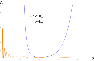
Figure 4: The trend of the probability density $\rho_{\phi}$ in function of the time $\phi$. The oscillatory $cos^{2}\left[ln\left(\phi\right)\right]$ regime is shown in orange; the hyperbolic $cosh^{2}\left[ln\left(\phi\right)\right]$ regime is shown in blue.

In particular, being $r>0$ and $k_{\alpha}<0$,

$$\begin{cases}\textnormal{if }r<-k_{\alpha}&\textnormal{oscillatory co$s^{2}\left[ln\left(\phi\right)\right]$ regime}\\ \textnormal{if }r>-k_{\alpha}&\textnormal{hyperbolic cos$h^{2}$}\left[ln\left(\phi\right)\right]\text{regime}\end{cases}$$ (113)

Considering the condition (61) derived from the Hamilton’s equations and the relation $p=\hbar k$, we conclude that only the oscillatory regime is physically acceptable. Therefore, the wave packet (98) can be rewritten as

$$\begin{array}[]{l}\Phi\left(\alpha,\beta_{\pm},\phi\right)\\ =\int_{-\infty}^{\;0}\int_{0}^{-k_{\alpha}}\int_{0}^{2\pi}dk_{\alpha}drd\theta\;\left[rA\left(k_{\alpha},r,\theta\right)\varphi\left(\alpha,\beta_{\pm},\phi\right)\right],\end{array}$$ (114)

where

$$\begin{array}[]{l}A\left(k_{\alpha},r,\theta\right)\\ =\cfrac{1}{\sqrt{\left(2\pi\right)^{3}}\sigma_{\alpha}\sigma_{+}\sigma_{-}}\;e^{-\left(\frac{\left(k_{\alpha}-\overline{k}_{\alpha}\right)^{2}}{2\sigma_{\alpha}^{2}}+\frac{\left(rsin\theta-\overline{rsin\theta}\right)^{2}}{2\sigma_{+}^{2}}+\frac{\left(rcos\theta-\overline{rcos\theta}\right)^{2}}{2\sigma_{-}^{2}}\right)}.\end{array}$$ (115)

Consequently, the normalizable probability density is

$$\rho_{\phi}=i\left(\Phi^{*}\partial_{\phi}\Phi-\Phi\partial_{\phi}\Phi^{*}\right).$$ (116)

XII The isotropic and homogeneous FLRW Universe

In this section, we will analyze the quantum behavior of the FLRW Universe in the context of the $f(R)$ gravity in the Jordan frame. In the assumption $\beta_{\pm}=0$ (and hence $p_{\pm}=0$) the superHamiltonian (53) reduces to the simpler form

$$\mathcal{H}_{FLRW,\,JF}=\cfrac{2e^{-\frac{3}{2}\alpha}}{\mathbf{v}}\left[\cfrac{1}{6}\pi_{\phi}^{2}\phi-\cfrac{1}{3}p_{\alpha}\pi_{\phi}\right],$$ (117)

and quantum dynamics is described by the Wheeler-De Witt equation

$$\cfrac{2e^{-\frac{3}{2}\alpha}}{\mathbf{v}}\hbar^{2}\left[-\cfrac{1}{6}\partial_{\phi}\left(\phi\partial_{\phi}\right)+\cfrac{1}{3}\partial_{\alpha}\partial_{\phi}\right]\varphi\left(\alpha,\phi\right)=0.$$ (118)

We note that the quantization of a homogeneous and isotropic model has no clear physical meaning, since we lost the two Einstenian gravitational degrees of freedom. In this respect, we can infer that the quantization of the FLRW Universe must be mainly regarded as a toy model on which the different quantum cosmology approaches can be easily tested. Considering the natural solution

$$\varphi=Ae^{ik_{\alpha}\alpha}f(\phi),$$ (119)

we obtain a second-order differential equation for the function $f(\phi)$

$$\phi\cfrac{\partial^{2}f}{\partial\phi^{2}}+\cfrac{\partial f}{\partial\phi}\left(1-2ik_{\alpha}\right)=0,$$ (120)

having as solution

$$f(\phi)=c_{1}+c_{2}\left(\cfrac{1}{2ik_{\alpha}}\right)\phi^{2ik_{\alpha}}.$$ (121)

XII.1 Time before quantization: the ADM reduction method

In the model under examination, we consider the variable $\phi$ as the embedding variable and the Misner variable $\alpha$ as the physical degree of freedom. Solving classically the superHamiltonian constraint with respect to the conjugate momentum $\pi_{\phi}$ we derive the equation

$$\pi_{\phi}\left(\cfrac{1}{6}\pi_{\phi}\phi-\cfrac{1}{3}p_{\alpha}\right)=0,$$ (122)

having as solutions

$$\left\{\begin{array}[]{l}\pi_{\phi,1}=0\\ \pi_{\phi,2}=\cfrac{2p_{\alpha}}{\phi}\end{array}\right.$$ (123)

Considering the non-trivial one, we can define

$$h_{\phi}=-\cfrac{2p_{\alpha}}{\phi},$$ (124)

as the physical Hamiltonian that regulates the dynamics with respect to the time $\phi$. The next step consists in the imposition of the so-called time gauge

$$\begin{array}[]{cl}\dot{\phi}&=N\cfrac{\partial\mathcal{H}_{FLRW,\,JF}}{\partial\pi_{\phi}}\\ &=\cfrac{2Ne^{-\frac{3}{2}\alpha}}{\mathbf{v}}\left(\cfrac{1}{3}\pi_{\phi}\phi-\cfrac{1}{3}p_{\alpha}\right)=1,\end{array}$$ (125)

which sets the the lapse function $N$

$$N=N_{ADM}=\cfrac{3\mathbf{v}e^{\frac{3}{2}\alpha}}{2\left(\pi_{\phi}\phi-p_{\alpha}\right)},$$ (126)

and allows us to write the reduced action

$$S_{red}=\int d\phi\left(p_{\alpha}\cfrac{\partial\alpha}{\partial\phi}-h_{\phi}\right),$$ (127)

The Hamilton’s equations are defined as

$$\left\{\begin{array}[]{c}\cfrac{\partial\alpha}{\partial\phi}=\cfrac{\partial h_{\phi}}{\partial p_{\alpha}}=-\cfrac{2}{\phi}\\ \cfrac{\partial p_{\alpha}}{\partial\phi}=-\cfrac{\partial h_{\phi}}{\partial\alpha}=0\end{array}\right.$$ (128)

from which we obtain the classical trajectory with respect to time $\phi$

$$\alpha(\phi)=-2ln\left(\phi\right)+\alpha_{0}=-2ln\left(\phi\right),$$ (129)

where we have set $\alpha_{0}=\alpha(0)=0$.

XII.2 The probability density and the comparison between the classical trajectory and the quantum evolution

In analogy to the case of the Bianchi I Universe we want to define a Hilbert space through the introduction of the probability density

$$\rho_{\phi}=i\left(\varphi^{*}\partial_{\phi}\varphi-\varphi\partial_{\phi}\varphi^{*}\right).$$ (130)

Replacing the wave function (119) assuming $c_{1}=0,c_{2}=1$, we obtain the non-normalized probability density

$$\rho_{\phi}=-\cfrac{1}{k_{\alpha}\phi},$$ (131)

which is positive if $k_{\alpha}<0$. Considering that there are no monochromatic physical wave functions, we construct the Gaussian wave packet which is a solution of the Wheeler-De Witt equation (118)

$$\Phi\left(\alpha,\phi\right)=\int_{-\infty}^{\,0}dk_{\alpha}A(k_{\alpha})e^{ik_{\alpha}\alpha}\left(\cfrac{1}{2ik_{\alpha}}\right)\phi^{2ik_{\alpha}},$$ (132)

where

$$A\left(k_{\alpha}\right)=\cfrac{1}{\sqrt{\left(2\pi\right)}\sigma_{\alpha}}\;e^{-\left(\frac{\left(k_{\alpha}-\bar{k}_{\alpha}\right)^{2}}{2\sigma_{\alpha}^{2}}\right)}.$$ (133)

The normalized probability density

$$\rho_{\phi}=i\left(\Phi^{*}\partial_{\phi}\Phi-\Phi\partial_{\phi}\Phi^{*}\right).$$ (134)

gives the probability of finding the FLRW Universe at a certain instant $\phi$ per unit of “spatial coordinate” $\alpha$.

We now study the trend of the quantity (134) with respect to $\phi>0$ as we can see from (129) (FIG.5).

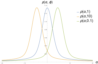
Figure 5: The trend of the probability density $\rho\left(\alpha,\phi\right)$ in function of the coordinate $\alpha$ for different values of $\phi$. $\phi=1$ is shown in blue; $\phi=\frac{1}{10}$ is shown in green; $\phi=1$0 is shown in orange.

From FIG.5 we see that there is no spreading of the wave packet and the probability density remains perfectly localized over time. We now prove the validity of the Ehrenfest Theorem by comparing the classical trajectory provided by Hamilton’s equations and the values of the coordinates $\alpha$ corresponding to the maximums of the probability density $\rho_{\phi}$ as $\phi$ varies. Strictly speaking, we should study the expectation value $<\Phi|\hat{\alpha}|\Phi>$, but for highly localized Gaussian probability density the values of $\alpha$ where there’s a maximum is a good approximation). From FIG.6 it is evident that the quantum dynamics perfectly follows the classical dynamics of the FLRW Universe in the Jordan frame. This result demonstrates that such a quantum-cosmological model reaches the singularity ($\phi\rightarrow+\infty$) in a classical way, allowing us to consider the quantum effects in the Planckian regime, as effects of lower order on a semiclassical Universe.

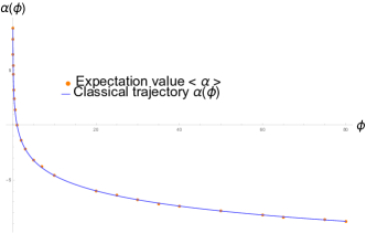
Figure 6: Comparison between the classical trajectory (solid blue line) and the values $\alpha\left(\phi\right)$ where the probability density is maximally localized as $\phi$ varies (dotted orange line).

XII.3 Comparison with the FLRW model filled with a scalar field in General Relativity

The Wheeler-De Witt equation in Misner variables for the FLRW Universe in GR filled with a minimally coupled scalar field $\phi$ is

$$\begin{array}[]{ccl}\mathcal{H}_{FLRW+\phi}&=&\cfrac{2e^{-\frac{3}{2}\alpha}}{\mathbf{v}}\left[-\hat{p}_{\alpha}^{2}+\hat{\pi}_{\phi}^{2}\right]|\varphi\rangle\\ &=&\cfrac{2e^{-\frac{3}{2}\alpha}}{\mathbf{v}}\left(\partial_{\alpha}^{2}-\partial_{\phi}^{2}\right)\varphi\left(\alpha,\phi\right)=0,\end{array}$$ (135)

where we neglected the potential term $V\left(\phi\right)$ related to the derivatives of the scalar field. Differently from the case (118) in the Jordan frame, this equation resembles a 2-dimensional Klein-Gordon equation describing a free and massless particle, where the external scalar field $\phi$ plays the role of the time variable. The wave function $\varphi$ solution of the equation is a plane wave

$$\varphi\left(\alpha,\phi\right)=Ae^{i\left(k_{\alpha}\alpha+k_{\phi}\phi\right)},$$ (136)

and assuming a Gaussian wave packet at the initial time $\phi_{0}$, we write the general solution

$$\Phi\left(\alpha,\phi\right)=\int_{-\infty}^{\,0}dkA(k)e^{ik\left(\alpha+\phi\right)}$$ (137)

where

$$A\left(k\right)=\cfrac{1}{\sqrt{\left(2\pi\right)}\sigma}\;e^{-\left(\frac{\left(k-\overline{k}\right)^{2}}{2\sigma^{2}}\right)},$$ (138)

and $k\equiv k_{\phi}=k_{\alpha}<0$. Through the study of the probability density

$$\rho_{\phi}=i\left(\Phi^{*}\partial_{\phi}\Phi-\Phi\partial_{\phi}\Phi^{*}\right),$$ (139)

we can infer the absence of the spreading phenomenon typical of a free quantum particle (FIG.7).

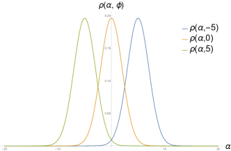
Figure 7: Evolution of the probability density $\rho\left(\alpha,\phi\right)$ in function of the coordinate $\alpha$ for different values of $\phi$. $\phi=0$ is shown in orange; $\phi=5$ is shown in green; $\phi=-5$ is shown in blue.

We conclude that even in the case of GR with a minimally coupled scalar field, the FLRW Universe admits a classical limit valid up to Planckian regimes. In support of this claim, we apply the ADM reduction procedure and derive the Hamilton’s equations

$$\left\{\begin{array}[]{l}\cfrac{\partial\alpha}{\partial\phi}=\cfrac{\partial h_{\phi}}{\partial p_{\alpha}}=-\cfrac{1}{2\sqrt{p_{\alpha}}},\\ \cfrac{\partial p_{\alpha}}{\partial\phi}=-\cfrac{\partial h_{\phi}}{\partial\alpha}=0,\end{array}\right.$$ (140)

from which the classical trajectory takes the form

$$\alpha\left(\phi\right)=-c\phi,$$ (141)

where $c$ is a constant of the motion.

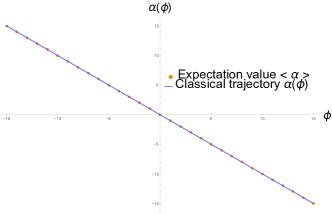
Figure 8: Comparison between the classical trajectory (solid blue line) and the values $\alpha\left(\phi\right)$ where the probability density is maximally localized as $\phi$ varies (dotted orange line).

From FIG.8 it emerges that quantum dynamics perfectly follows the classical dynamics of the FLRW Universe filled with a minimally coupled scalar field. Furthermore, it is possible to fix the constant of motion $c=1$. In conclusion, we stress two main differences between the two models under consideration: the first one is the linear vs. logarithmic trend of $\alpha\left(\phi\right)$ with which the singularity is approached; the second one is the range of values assumed by the time variable $\phi$ which, in the case of the Jordan frame, was limited only to the positive semi-axis of the Real numbers. In both models, however, the canonical quantization based on the Wheeler-De Witt formalism does not solve the problem of the existence of a cosmological singularity, paving the way for different theoretical approaches.

Part VII Concluding remarks

In this paper, we provided a systematic and detailed analysis of the cosmological implication of an $f(R)$-gravity in the Jordan frame, especially in the limit of a negligible potential term of the non-minimally coupled scalar field. Some interesting results have been clearly stated and here briefly re-analyzed. As first step, we show in the general Hamiltonian formulation, as well as in its implementation to the dynamics of a generic universe, that if we use the 3-metric determinant as a separated variable, like in [15], its conjugate momentum enters linearly only in the scalar Hamiltonian constraint. Differently from what it takes place in the standard Wheeler-DeWitt equation, we are here always able to set up a Schröedinger formulation in which the 3-determinant plays the role of a time variable, although the associated Hamiltonian turns out to be a non-local functional operator. The second very significant result we developed consists of the proof that the Bianchi IX cosmology is no longer characterized by a chaotic dynamics in an extended $f(R)$ theory of gravity, as soon as the potential term bringing the information on the form of $f$ is negligible near to the singularity. Here we adopted Minser variables to describe the Bianchi IX line element and we demonstrated both the existence and the actractivity of a Kasner stability region. The definition of the region where a Kasner regime becomes stable is derived analytically, while the proof that the system always reaches such a configuration has been performed on a numerical level. This latter study relies on the existence of three constants of the motion and it can be regarded as the natural generalization of the original Misner approach [23]. The result obtained here about the chaos suppression is coherent with the analysis in [11], where the same issue is discussed using a $f(R)$ approach in the so-called Einstein framework and adopting Misner-Chitré-like variables. Finally, we touch the question of the canonical quantization of the Bianchi I dynamics, concentrating our attention to the quantum evolution of an isotropic Universe. For the Bianchi I Wheeler-DeWitt equation a conserved current is constructed and a probability density is identified by interpreting the non-minimal scalar field as the internal time variable. A localized wave packet is then constructed for the isotropic universe and we show how the singularity is still present in such a quantum scenario. Furthermore a comparison between the evolutionary cosmologies using as internal time a minimally and a non-minimally coupled scalar field respectively is provided. Apart from a different dynamics of the peak of the localized packet, we clarify how the non-minimally coupled scalar field emerging in a Jordan frame is a valuable internal time and opens a new point of view on the interpretation of modified $f(R)$ theory of gravity: the additional scalar mode, summarizing the functional form $f$, can be interpreted as a time-like degree of freedom for the gravitational quantum dynamics, although a viable approach could also emerge by dealing, as stressed above, with the 3-metric determinant. Since the Bianchi model dynamics has paradigmatic features of the generic inhomogeneous cosmology, we are lead to infer that the present analysis has a relevant impact on a more general sector of the cosmological problem. However, it must be recalled that, when the potential term associated to the non-minimally coupled scalar field is no longer negligible near the singularity, its presence can significantly affect the validity of some of the present issues, including the non-chaoticity of the Bianchi IX Universe.

XIII Appendix A

We explicit the canonical transformation used in Part IV, sec.VI

$$\begin{array}[]{l}p^{ij}\partial_{t}h_{ij}\\ =\underset{a}{\sum}p_{a}\partial_{t}q_{a}\,+\,\underset{a}{\sum}\pi_{a}\partial_{t}y_{a}\\ p^{ij}\partial_{t}\left(\underset{a}{\sum}e^{q_{a}}e_{i}^{a}e_{j}^{a}\right)\\ =\underset{a}{\sum}p_{a}\partial_{t}q_{a}\,+\,\underset{a}{\sum}\pi_{a}\partial_{t}y_{a}\\ p^{ij}\underset{a}{\sum}\partial_{t}q_{a}e^{q_{a}}e_{i}^{a}e_{j}^{a}+2p^{ij}\underset{a}{\sum}e^{q_{a}}e_{i}^{a}\partial_{t}e_{j}^{a}\\ =\underset{a}{\sum}p_{a}\partial_{t}q_{a}\,+\,\underset{a}{\sum}\pi_{a}\partial_{t}y_{a}\\ p^{ij}\underset{a}{\sum}\partial_{t}q_{a}e^{q_{a}}e_{i}^{a}e_{j}^{a}+2p^{ij}\underset{a}{\sum}e^{q_{a}}e_{i}^{a}\partial_{t}\left(O_{c}^{a}\partial_{j}y^{c}\right)\\ =\underset{a}{\sum}p_{a}\partial_{t}q_{a}\,+\,\underset{a}{\sum}\pi_{a}\partial_{t}y_{a}\\ p^{ij}\underset{a}{\sum}\partial_{t}q_{a}e^{q_{a}}e_{i}^{a}e_{j}^{a}+\partial_{j}\left(2p^{ij}\underset{a}{\sum}e^{q_{a}}e_{i}^{a}\partial_{t}y^{c}O_{c}^{a}\right)\\ -\partial_{j}\left(2p^{ij}\underset{a}{\sum}e^{q_{a}}e_{i}^{a}O_{c}^{a}\right)\partial_{t}y^{c}\\ =\underset{a}{\sum}p_{a}\partial_{t}q_{a}\,+\,\underset{a}{\sum}\pi_{a}\partial_{t}y_{a}\\ p^{ij}\underset{a}{\sum}\partial_{t}q_{a}e^{q_{a}}e_{i}^{a}e_{j}^{a}-\underset{a}{\sum}\partial_{j}\left(2p^{ij}e^{q_{a}}e_{i}^{a}O_{c}^{a}\right)\partial_{t}y^{c}\\ =\underset{a}{\sum}p_{a}\partial_{t}q_{a}\,+\,\underset{a}{\sum}\pi_{a}\partial_{t}y_{a}\end{array}$$ (142)

where we neglected the the term $\partial_{j}\left(2p^{ij}\underset{a}{\sum}e^{q_{a}}e_{i}^{a}\partial_{t}y^{c}O_{c}^{a}\right)$, because $p^{ij}$ is a tensor density. From the definition of the superHamiltonian of gravity in the Jordan frame

$$\mathcal{H}_{g,JF} =\cfrac{2}{\sqrt{h}}\left(\cfrac{p_{ij}p^{ij}-\frac{1}{3}p^{2}}{\phi}+\cfrac{1}{6}\phi\pi_{\phi}^{2}-\cfrac{1}{3}p\pi_{\phi}\right)$$

$$\quad+\cfrac{\sqrt{h}}{2}\left(V(\phi)-\phi\,^{3}R+2D_{i}D^{i}\phi\right)$$ (143)

we replace the relationships

$$p^{ij}p_{ij} =\underset{a}{\sum}e^{-q_{a}}p_{a}e_{a}^{i}e_{a}^{j}\underset{b}{\sum}e^{q_{b}}p_{b}e_{i}^{b}e_{j}^{b}$$

$$=\underset{a}{\sum}\underset{b}{\sum}e^{-q_{a}}e^{q_{b}}p_{a}p_{b}\delta_{a}^{b}e_{a}^{j}e_{j}^{b}$$

$$=\underset{a}{\sum}p_{a}^{2}$$ (144)

$$p^{2} =\left(h_{ij}p^{ij}\right)^{2}$$

$$=\left(\underset{a}{\sum}e^{q_{a}}e_{i}^{a}e_{j}^{a}\underset{b}{\sum}e^{-q_{b}}p_{b}e_{b}^{i}e_{b}^{j}\right)^{2}$$

$$=\left(\underset{a}{\sum}\underset{b}{\sum}e^{q_{a}}e^{-q_{b}}p_{b}\delta_{b}^{a}e_{j}^{a}e_{b}^{j}\right)^{2}$$

$$=\left(\underset{a}{\sum}p_{a}\right)^{2}$$ (145)

in the kinetic term of the superHamiltonian obtaining the superHamiltonian (47)

$$\mathscr{H}_{g,JF} =\cfrac{2}{\sqrt{h}}\left(\cfrac{\underset{a}{\sum}p_{a}^{2}-\frac{1}{3}\left(\underset{a}{\sum}p_{a}\right)^{2}}{\phi}+\cfrac{1}{6}\phi\pi_{\phi}^{2}-\cfrac{1}{3}\underset{a}{\sum}p_{a}\pi_{\phi}\right)$$

$$\quad+\cfrac{\sqrt{h}}{2}\left(V(\phi)-\phi\,^{3}R+2D_{i}D^{i}\phi\right)$$ (146)

In order to obtain the supermomentum (48), we redefine the supermomentum of gravity in the Jordan frame

$$\mathcal{H}_{i}^{g,JF}=-2D_{j}p_{i}^{j}+\pi_{\phi}\partial_{i}\phi$$ (147)

and rewriting $p_{i}^{j}=\sqrt{h}T_{i}^{j}$ we get

$$\mathcal{H}_{i}^{g} -\pi_{\phi}\partial_{i}\phi$$

$$=-2\left(\partial_{j}p_{i}^{j}-\Gamma_{ij}^{l}p_{l}^{j}\right)$$

$$=-2\left[\partial_{j}\left(\underset{a}{\sum}p_{a}e_{i}^{a}e_{a}^{j}\right)-\Gamma_{ij}^{l}p_{l}^{j}\right]$$

$$=-2\left[\partial_{j}\left(\underset{a}{\sum}p_{a}e_{i}^{a}e_{a}^{j}\right)-\cfrac{1}{2}\left(\partial_{i}h_{jl}+\partial_{j}h_{il}-\partial_{l}h_{ij}\right)p^{jl}\right]$$

$$=-2\left[\partial_{j}\left(\underset{a}{\sum}p_{a}e_{i}^{a}e_{a}^{j}\right)-\cfrac{1}{2}\left(\partial_{i}h_{jl}\right)p^{jl}\right]$$

$$=-2\underset{a}{\sum}\left(\partial_{j}p_{a}\delta_{j}^{i}+p_{a}\partial_{j}\left(e_{a}^{j}O_{b}^{a}\partial_{i}y^{b}\right)\right)$$

$$\quad+\partial_{i}\left(\underset{d}{\sum}e^{q_{d}}e_{j}^{d}e_{l}^{d}\right)\underset{c}{\sum}e^{-q_{c}}p_{c}e_{c}^{j}e_{c}^{l}$$

$$=-2\underset{a}{\sum}\left(\partial_{i}p_{a}+p_{a}\partial_{j}\left(e_{a}^{j}O_{b}^{a}\right)\partial_{i}y^{b}+p_{a}e_{a}^{j}O_{b}^{a}\partial_{j}\partial_{i}y^{b}\right)$$

$$\quad+\underset{c}{\sum}\left(\partial_{i}q_{c}e^{q_{c}}e_{j}^{c}e_{l}^{c}e^{-q_{c}}p_{c}e_{c}^{j}e_{c}^{l}\right)+$$

$$\quad+\underset{c}{\sum}\left(e^{q_{c}}\partial_{i}\left(e_{j}^{c}\right)e_{l}^{c}e^{-q_{c}}p_{c}e_{c}^{j}e_{c}^{l}\right)+\underset{c}{\sum}e^{q_{c}}e_{j}^{d}\partial_{i}\left(e_{l}^{c}\right)e^{-q_{c}}p_{c}e_{c}^{j}e_{c}^{l}$$

$$=-2\underset{a}{\sum}\left(\partial_{i}p_{a}+p_{a}\partial_{j}\left(e_{a}^{j}O_{b}^{a}\right)\partial_{i}y^{b}+p_{a}e_{a}^{j}O_{b}^{a}\partial_{j}\partial_{i}y^{b}\right)$$

$$+\underset{c}{\sum}\left(p_{c}\partial_{i}q_{c}+2p_{c}\partial_{i}\left(O_{d}^{c}\partial_{l}y^{d}\right)e_{c}^{l}\right)$$

$$=-2\underset{a}{\sum}\left(\partial_{i}p_{a}+p_{a}\partial_{j}\left(e_{a}^{j}O_{b}^{a}\right)\partial_{i}y^{b}+p_{a}e_{a}^{j}O_{b}^{a}\partial_{j}\partial_{i}y^{b}\right)$$

$$\quad+\underset{c}{\sum}p_{c}\partial_{i}q_{c}++2\underset{c}{\sum}p_{c}\partial_{i}O_{d}^{c}\left(\partial_{l}y^{d}e_{c}^{l}\right)$$

$$\quad+2\underset{c}{\sum}p_{c}O_{d}^{c}\partial_{i}\partial_{l}y^{d}e_{c}^{l}$$

$$=-2\underset{a}{\sum}\left(\partial_{i}p_{a}+p_{a}\partial_{j}\left(e_{a}^{j}O_{b}^{a}\right)\partial_{i}y^{b}\right)$$

$$\quad-2\underset{a}{\sum}\left(p_{a}e_{a}^{j}O_{b}^{a}\partial_{j}\partial_{i}y^{b}+p_{a}e_{a}^{l}O_{d}^{a}\partial_{i}\partial_{l}y^{d}\right)+$$

$$\quad+\underset{c}{\sum}p_{c}\partial_{i}q_{c}+2\underset{c}{\sum}p_{c}\partial_{i}O_{d}^{c}\left(O^{-1}\right)_{c}^{d}$$

$$=-2\underset{a}{\sum}\left(\partial_{i}p_{a}+p_{a}\partial_{j}\left(e_{a}^{j}O_{b}^{a}\right)\partial_{i}y^{b}\right)$$

$$\quad+\underset{c}{\sum}p_{c}\partial_{i}q_{c}+2\underset{c}{\sum}p_{c}\partial_{i}O_{d}^{c}\left(O^{-1}\right)_{c}^{d}$$ (148)

From (142) we define

$$\pi_{c} =-2\underset{a}{\sum}\partial_{j}\left(p_{a}e_{a}^{j}(t,x^{k})O_{c}^{a}(x^{k})\right)$$

$$=-2\underset{a}{\sum}\left(\partial_{j}p_{a}O_{c}^{a}O_{a}^{d}\cfrac{\partial x^{j}}{\partial y^{d}}+p_{a}\partial_{j}O_{c}^{a}e_{a}^{j}+p_{a}O_{c}^{a}\partial_{j}e_{a}^{j}\right)$$

$$=-2\underset{a}{\sum}\left(\partial_{j}p_{a}\cfrac{\partial x^{j}}{\partial y^{c}}+p_{a}\partial_{j}O_{c}^{a}e_{a}^{j}+p_{a}O_{c}^{a}\partial_{j}e_{a}^{j}\right)$$ (149)

from which

$$\pi_{c}\partial_{i}y^{c} =-2\underset{a}{\sum}\left(\partial_{j}p_{a}\cfrac{\partial x^{j}}{\partial y^{c}}+p_{a}\partial_{j}O_{c}^{a}e_{a}^{j}+p_{a}O_{c}^{a}\partial_{j}e_{a}^{j}\right)\cfrac{\partial y^{c}}{\partial x^{i}}$$

$$=-2\underset{a}{\sum}\left(\partial_{i}p_{a}+p_{a}\partial_{j}O_{c}^{a}e_{a}^{j}\partial_{i}y^{c}+p_{a}O_{c}^{a}\partial_{j}e_{a}^{j}\partial_{i}y^{c}\right)$$

$$=-2\underset{a}{\sum}\left(\partial_{i}p_{a}+p_{a}\partial_{j}\left(e_{a}^{j}O_{c}^{a}\right)\partial_{i}y^{c}\right)$$ (150)

We, finally, find the supermomentum in the general framework (48)

$$\mathscr{H}_{i,JF}^{B}=\pi_{\phi}\partial_{i}\phi+\pi_{a}\partial_{i}y^{a}+p_{a}\partial_{i}q^{a}+2p_{a}\left(O^{-1}\right)_{a}^{b}\partial_{i}O_{b}^{a}$$ (151)

XIV Appendix B

As we have seen in section X, we have defined a stability region within which we are sure that the particle-Universe doesn’t impact with the potential wall, scattering from a Kasner solution to another. The calculation of the boundaries of the Kasner stability region was performed with the help of Wolfram Mathematica.

Now we want to describe the complete solutions:

$$\Biggl{\{}\begin{array}[]{l}-1<\beta_{+}^{{}^{\prime}}<0\\ \beta_{-}^{{}^{\prime}}>Root\left[Ax^{3}+Bx^{2}+Cx+D\right]\\ \beta_{-}^{{}^{\prime}}<Root\left[Ax^{3}-Bx^{2}+Cx-D\right]\end{array}$$ (152)

$$\Biggl{\{}\begin{array}[]{l}\beta_{+}^{{}^{\prime}}=0\\ \beta_{-}^{{}^{\prime}}>Root\left[1+3x^{2}+4\sqrt{3}x^{3}\right]\\ \beta_{-}^{{}^{\prime}}<Root\left[-1-3x^{2}+4\sqrt{3}x^{3}\right]\end{array}$$ (153)

$$\Biggl{\{}\begin{array}[]{l}0<\beta_{+}^{{}^{\prime}}<\frac{1}{2}\\ \beta_{-}^{{}^{\prime}}>Root\left[Ax^{3}+Bx^{2}+Cx+D\right]\\ \beta_{-}^{{}^{\prime}}<Root\left[Ax^{3}-Bx^{2}+Cx-D\right]\end{array}$$ (154)

$$\Biggl{\{}\begin{array}[]{l}\frac{1}{2}<\beta_{+}^{{}^{\prime}}<Root\left[-1-3x^{2}+8x^{3}\right]\\ -\sqrt{\frac{1+3v_{+}^{2}-8v_{+}^{3}}{-3+8v_{+}}}<\beta_{-}^{{}^{\prime}}<\sqrt{\frac{1+3v_{+}^{2}-8v_{+}^{3}}{-3+8v_{+}}}\end{array}$$ (155)

with: $A=4\sqrt{3},B=3+4v_{+},C=4\sqrt{3}$ and $D=1+3v_{+}^{2}+4v_{+}^{3}$.

References

- Kolb E. [1990] T. M. Kolb E., The early Universe (CRC Press, 1990).
- Cianfrani et al. [2014] F. Cianfrani, O. M. Lecian, M. Lulli, and G. Montani, Canonical Quantum Gravity: Fundamentals and Recent Developments (World Scientific, 2014).
- Montani et al. [2011] G. Montani, M. V. Battisti, R. Benini, and G. Imponente, Primordial cosmology (World Scientific, 2011).
- Thorne et al. [2000] K. S. Thorne, C. W. Misner, and J. A. Wheeler, Gravitation (Freeman, 2000).
- Landau [2013] L. D. Landau, The classical theory of fields, Vol. 2 (Elsevier, 2013).
- Belinskii et al. [1982] V. Belinskii, I. Khalatnikov, and E. Lifshitz, A general solution of the einstein equations with a time singularity, Advances in Physics 31, 639 (1982), https://doi.org/10.1080/00018738200101428 .
- Belinskij et al. [1970] V. A. Belinskij, I. M. Khalatnikov, and E. M. Lifshits, Oscillatory approach to a singular point in the relativistic cosmology., Advances in Physics 19, 525 (1970).
- Sotiriou and Faraoni [2010] T. P. Sotiriou and V. Faraoni, theories of gravity, Rev. Mod. Phys. 82, 451 (2010).
- Bamba et al. [2012] K. Bamba, S. Capozziello, S. Nojiri, and S. D. Odintsov, Dark energy cosmology: the equivalent description via different theoretical models and cosmography tests, Astrophysics and Space Science 342, 155–228 (2012).
- Capozziello et al. [2013] S. Capozziello, N. Carlevaro, M. De Laurentis, M. Lattanzi, and G. Montani, Cosmological implications of a viable non-analytical f(R) model, European Physical Journal Plus 128, 155 (2013).
- Moriconi et al. [2014] R. Moriconi, G. Montani, and S. Capozziello, Chaos removal in gravity: The mixmaster model, Phys. Rev. D 90, 101503 (2014).
- Lecian and Montani [2012] O. M. Lecian and G. Montani, Exponential lagrangian for the gravitational field and the problem of vacuum energy, International Journal of Modern Physics A 23 (2012).
- Nojiri and Odintsov [2011] S. Nojiri and S. D. Odintsov, Unified cosmic history in modified gravity: From F(R) theory to Lorentz non-invariant models, physrep 505, 59 (2011), arXiv:1011.0544 [gr-qc] .
- Zhang and Ma [2011] X. Zhang and Y. Ma, Extension of loop quantum gravity to theories, Phys. Rev. Lett. 106, 171301 (2011).
- DeWitt [1967] B. S. DeWitt, Quantum theory of gravity. i. the canonical theory, Phys. Rev. 160, 1113 (1967).
- Arnowitt et al. [1960] R. Arnowitt, S. Deser, and C. W. Misner, Canonical variables for general relativity, Phys. Rev. 117, 1595 (1960).
- Kirillov [1993] A. Kirillov, On the question of the characteristics of the spatial distribution of metric inhomogeneities in a general solution to einstein equations in the vicinity of a cosmological singularity, Zhurnal Eksperimental noi i Teoreticheskoi Fiziki 103, 721 (1993).
- Imponente and Montani [2002] G. Imponente and G. Montani, On the quantum origin of the mixmaster chaos covariance, Nuclear Physics B - Proceedings Supplements 104, 193 (2002).
- Montani et al. [2008] G. Montani, M. V. Battisti, R. Benini, and G. Imponente, Classical and Quantum Features of the Mixmaster Singularity, International Journal of Modern Physics A 23, 2353 (2008), arXiv:0712.3008 [gr-qc] .
- Deruelle et al. [2009] N. Deruelle, Y. Sendouda, and A. Youssef, Various hamiltonian formulations of gravity and their canonical relationships, Phys. Rev. D 80, 084032 (2009).
- Bombacigno et al. [2021] F. Bombacigno, S. Boudet, and G. Montani, Generalized Ashtekar variables for Palatini models, Nucl. Phys. B 963, 115281 (2021), arXiv:1911.09066 [gr-qc] .
- Misner [1969a] C. W. Misner, Mixmaster universe, Phys. Rev. Lett. 22, 1071 (1969a).
- Misner [1969b] C. W. Misner, Quantum cosmology. i, Phys. Rev. 186, 1319 (1969b).
- Berger [1999] B. K. Berger, Influence of scalar fields on the approach to a cosmological singularity, Phys. Rev. D 61, 023508 (1999).