Weighted SPICE Algorithms for Range-Doppler Imaging Using One-Bit Automotive Radar

Abstract

We consider the problem of range-Doppler imaging using one-bit automotive LFMCW or PMCW radar that utilizes one-bit ADC sampling with time-varying thresholds at the receiver. The one-bit sampling technique can significantly reduce the cost as well as the power consumption of automotive radar systems. We formulate the one-bit LFMCW/PMCW radar range-Doppler imaging problem as one-bit sparse parameter estimation. The recently proposed hyperparameter-free (and hence user friendly) weighted SPICE algorithms, including SPICE, LIKES, SLIM and IAA, achieve excellent parameter estimation performance for data sampled with high precision. However, these algorithms cannot be used directly for one-bit data. In this paper we first present a regularized minimization algorithm, referred to as 1bSLIM, for accurate range-Doppler imaging using one-bit radar systems. Then, we describe how to extend the SPICE, LIKES and IAA algorithms to the one-bit data case, and refer to these extensions as 1bSPICE, 1bLIKES and 1bIAA. These one-bit hyperparameter-free algorithms are unified within the one-bit weighted SPICE framework. Moreover, efficient implementations of the aforementioned algorithms are investigated that rely heavily on the use of FFTs. Finally, both simulated and experimental examples are provided to demonstrate the effectiveness of the proposed algorithms for range-Doppler imaging using one-bit automotive radar systems.

I Introduction

Millimeter wave radar is widely used in diverse applications including advanced driver assistance automotive systems and fully autonomous vehicles [1]. Compared with other sensing systems, such as cameras, lidars and ultrasonics, radar systems can provide better performance, especially in poor lighting or adverse weather conditions [2].
The most commonly used probing waveform in existing commercial automotive radar systems is the LFMCW waveform, which reduces the system cost by allowing low-rate ADCs at the radar receivers. An LFMCW radar system transmits a series of chirps, which are reflected by the targets and mixed with the transmitted chirp at the receiver. The range or range-Doppler estimation problem is converted to a 1-D or 2-D complex sinusoidal parameter estimation problem [3, 4]. However, mutual interferences among LFMCW automotive radars become more severe as these radar systems become more widely used, since they occupy the same 77-81 GHz band. PMCW waveforms can be used to mitigate the interference problems. To reduce costs, binary sequences with desirable auto- and cross-correlation properties have been designed for PMCW automotive radars (see, e.g., [5] and the references therein). The flexibility and diversity offered by binary sequences allow the PMCW radars to mitigate mutual interferences similar to the CDMA communication systems [6]. Also, near orthogonality can be realized in the coding domain, which is advantageous for MIMO operations [7, 8].
To improve the range resolution of automotive radars, the fundamental approach is to increase the bandwidth of the transmitted signal, which can increase the ADC cost and power consumption. For example, a PMCW radar usually performs demodulation in the digital domain [9]. A PMCW radar with a chip rate of 2 GHz requires a sampling rate of at least 2 GHz [10]. However, an ADC with high precision quantization and high sampling rate is both expensive and power hungry. Yet low cost and low power consumption are crucial for commercial radar systems such as automotive radar.
One-bit sampling is a promising technique to mitigate the aforementioned ADC problems because of its low cost and low power consumption advantages. Due to these attractive properties, one-bit sampling has been considered for radar sensing [11, 12], spectral estimation [13, 14, 15], as well as massive MIMO communications [16, 17, 18]. The conventional one-bit sampling considered in, e.g., [19, 20, 21], compares the original signal with a zero threshold, which results in a loss of signal amplitude information. Recently, time-varying thresholds have been considered for one-bit sampling to achieve accurate amplitude estimation [22, 15]. In such a case, signed measurements are obtained by comparing the received signal with a known time-varying threshold.
In this paper, we consider one-bit sampling with time-varying thresholds for automotive radars to reduce cost and power consumption. We formulate the one-bit range-Doppler estimation problem as a one-bit sparse parameter estimation problem. Sparse parameter estimation using high-precision data has attracted much attention in the last two decades. Many algorithms have been developed with the goal of obtaining accurate sparse parameter estimates. Among them, the unified weighted SPICE algorithms [23], including SPICE [24], LIKES [25], SLIM [26] and IAA [27, 28, 29], do not require the tuning of any user-parameter and hence are easy to use in practice. These algorithms yield excellent estimation performance, in particular they possess high resolution and low sidelobe properties. Furthermore, IAA works well in various environments and the robustness of IAA has been ranked high in a recent review article [30]. However, these algorithms, together with the conventional FFT, cannot be used directly to solve one-bit sparse parameter estimation problems. Herein, we first present a regularized minimization algorithm, referred to as 1bSLIM, for accurate range-Doppler imaging using one-bit automotive radar. Additionally, we show that 1bSLIM, devised by means of a majorization-minimization approach [31, 32, 33, 34, 35], can be interpreted as applying the conventional SLIM algorithm to certain modified high-precision data. Inspired by this relationship, we describe how to extend SPICE, LIKES and IAA to the one-bit case, and refer to these extensions as 1bSPICE, 1bLIKES and 1bIAA. Each of the algorithms we present herein has its own merits and may be preferred in a specific application. Similar to the original weighted SPICE algorithms, which unify SPICE, LIKES, SLIM and IAA under the same weighted SPICE umbrella, the aforementioned one-bit algorithms are unified within the one-bit weighted SPICE framework. Moreover, these four one-bit algorithms are all hyperparameter-free and thus are easy to use in practice. Finally, simulated and experimental examples are provided to demonstrate the effectiveness of the proposed algorithms for range-Doppler imaging using one-bit automotive radars.
Notation: We denote vectors and matrices by bold lowercase and uppercase letters, respectively. $(\cdot)^{T}$ and $(\cdot)^{H}$ represent the transpose and the conjugate transpose, respectively. $\boldsymbol{R}\in\mathbb{R}^{N\times M}$ or $\boldsymbol{R}\in\mathbb{C}^{N\times M}$ denotes a real or complex-valued $N\times M$ matrix $\boldsymbol{R}$. $\otimes$ denotes the Kronecker matrix product. ${\rm vec}(\cdot)$ refers to the column-wise vectorization operation and ${\rm diag}(\boldsymbol{d})$ denotes a diagonal matrix with diagonal entries formed from $\boldsymbol{d}$. $\|\cdot\|$ and $\|\cdot\|_{F}$ are, respectively, the $\ell_{2}$ and Frobenius norms of vectors and matrices. ${\rm tr}\{\boldsymbol{R}\}$ and $\left|\boldsymbol{R}\right|$, respectively, denote the trace and determinant of a square matrix $\boldsymbol{R}$. $\boldsymbol{A}\preceq\boldsymbol{B}$ means that $\boldsymbol{B}-\boldsymbol{A}$ is a positive semidefinite matrix. ${\rm Re}[x]$ and ${\rm Im}[x]$ denote the real- and imaginary-parts of $x$. $x$ mod $N$ is the remainder of the Euclidean division of $x$ by $N$. Finally, $j=\sqrt{-1}$.
Throughout this paper, we use the following abbreviations:

ADC	Analog-to-digital converter
AGC	Automatic gain control
CDMA	Code division multiple access
CGLS	Conjugate-gradient least squares
CPI	Coherent processing interval
DAC	Digital-to-analog converter
DFT	Discrete Fourier transform
FFT	Fast Fourier transform
IAA	Iterative adaptive approach
LIKES	Likelihood-based estimation of sparse parameters
LFMCW	Linear frequency-modulated continuous-wave
LMMSE	Linear minimum mean square error
MAP	Maximum a posteriori
MIMO	Multiple-input multiple-output
MM	Majorization-minimization
NMSE	Normalized mean-squared error
PMCW	Phase-modulated continuous-wave
PRI	Pulse repetition interval
SLIM	Sparse learning via iterative minimization
SPICE	Sparse iterative covariance-based estimation
SNR	Signal-to-noise ratio

II Problem Formulation

In this section, we first briefly describe the signal models for the LFMCW and PMCW radars. Then, using the signed measurements obtained by one-bit sampling with time-varying thresholds, we formulate the range-Doppler imaging problem as a sparse parameter estimation problem.

II-A LFMCW Radar

Without loss of generality, we consider an LFMCW single-input single-output radar. A simplified model for the received signal (after dechirping and pre-processing) is as follows (see e.g., [11]):

$$y(n_{1},n_{2})=\sum_{k_{\rm d}=1}^{K_{\rm d}}\sum_{k_{\rm r}=1}^{K_{\rm r}}\gamma_{k_{\rm r},k_{\rm d}}e^{j(\omega_{k_{\rm r}}n_{1}+\bar{\omega}_{k_{\rm d}}n_{2})}+e(n_{1},n_{2}),$$ (1)

where $K_{\rm r}$ and $K_{\rm d}$ are the numbers of the grid points in the range and Doppler domains, respectively; the fast-time index $n_{1},n_{1}=1,2,\dots,N_{1}$, corresponds to the $n_{1}$th sample within a chirp; the slow-time index $n_{2},n_{2}=1,2,\dots,N_{2}$, is for the $n_{2}$th chirp; $\gamma_{k_{\rm r},k_{\rm d}}$ represents the reflection coefficient of a scatterer corresponding to the frequency pair $(\omega_{k_{\rm r}},\bar{\omega}_{k_{\rm d}})$; and $e(n_{1},n_{2})$ is the unknown additive noise. The frequency pair $(\omega_{k_{\rm r}},\bar{\omega}_{k_{\rm d}})$ is approximately related to the range-Doppler pair $(R_{k_{\rm r}},v_{k_{\rm d}})$ through the following equations:

$$\omega_{k_{\rm r}}=2\pi\left(\frac{4\mu R_{k_{\rm r}}}{cf_{\rm s}}+\frac{2f_{0}v_{k_{\rm d}}}{cf_{\rm s}}\right),\quad\bar{\omega}_{k_{\rm d}}=\frac{4\pi f_{0}v_{k_{\rm d}}T_{\rm c}}{c},$$ (2)

where $2\mu$ is the chirp rate; $c$ is the speed of light; $f_{\rm s}$ is the sampling frequency; $f_{0}$ denotes the carrier frequency; and $T_{\rm c}$ is the chirp duration. The range-Doppler information can therefore be recovered from the frequency pair $(\omega_{k_{\rm r}},\bar{\omega}_{k_{\rm d}})$ by using Equation (2). The range-Doppler estimation problem associated with (1) for an LFMCW radar is equivalent to a 2-D complex-valued sinusoidal parameter estimation problem. Let the measurement vector be denoted $\boldsymbol{y}=\begin{bmatrix}y(1,1),y(2,1),\dots,y(N_{1},N_{2})\end{bmatrix}^{T}$ and let $\boldsymbol{e}$ denote the unknown noise vector. Let the unknown parameter vector be denoted $\boldsymbol{\gamma}=\begin{bmatrix}\gamma_{1,1},\gamma_{2,1},\dots,\gamma_{K_{\rm r},K_{\rm d}}\end{bmatrix}^{T}$. Equation (1) can then be reformulated as:

$$\boldsymbol{y}=\boldsymbol{B}\boldsymbol{\gamma}+\boldsymbol{e}\in\mathbb{C}^{N},\quad\boldsymbol{B}\in\mathbb{C}^{N\times M},\quad M\gg N,$$ (3)

where $N=N_{1}N_{2}$ and $M=K_{\rm r}K_{\rm d}$. $K_{\rm r}\gg N_{1}$ and $K_{\rm d}\gg N_{2}$ are typical assumptions used by sparse parameter estimation algorithms to form a sufficiently fine grid, which enables us to obtain high resolution spectral estimates and excellent results even when the true target frequencies do not lie on the grid. Let $\boldsymbol{\psi}_{N}(\omega)=\begin{bmatrix}1,\ e^{j\omega},\dots,e^{j(N-1)\omega}\end{bmatrix}^{T}$. Then, the columns of $\boldsymbol{B}$ are given by $\{\boldsymbol{\psi}_{N_{1},N_{2}}\left(\omega_{k_{\rm r}},\bar{\omega}_{k_{\rm d}}\right)\}_{k_{\rm r}=1,k_{\rm d}=1}^{K_{\rm r},K_{\rm d}}$ with $\boldsymbol{\psi}_{N_{1},N_{2}}(\omega_{k_{\rm r}},\bar{\omega}_{k_{\rm d}})=\boldsymbol{\psi}_{N_{2}}(\bar{\omega}_{k_{\rm d}})\otimes\boldsymbol{\psi}_{N_{1}}(\omega_{k_{\rm r}})$.

For radar range-Doppler imaging applications, the number of potential scatterers of interest in a scene is usually much smaller than the number of grid points, which means that most of the elements in $\boldsymbol{\gamma}$ will be zero. Hence, the LFMCW radar range-Doppler imaging problem in (3) can be treated as a sparse parameter estimation problem.

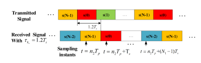
Figure 1: The transmitted sequence and the received sequence with $\tau_{k_{r}}=1.2T_{s}$.

II-B PMCW Radar

The PMCW radar periodically transmits a binary sequence $\boldsymbol{s}\!=\begin{bmatrix}s(0),\ s(1),\dots,s(N_{1}-1)\end{bmatrix}^{T}$, where $N_{1}$ is the sequence length and each element of $\boldsymbol{s}$ is either $1$ or $-1$, i.e., $s(n_{1})\in\{1,-1\}$. Then, the transmitted baseband signal can be written as:

$$x(t)=\sum_{n_{2}=-\infty}^{\infty}\sum_{n_{1}=0}^{N_{1}-1}s(n_{1})p(t-n_{1}T_{\rm s}-n_{2}T_{\rm p}),$$ (4)

where $T_{\rm s}$ is the so-called chip duration; $T_{\rm p}=N_{1}T_{\rm s}$ is the PRI; and $p(t)$ is the impulse response of a pulse-shaping filter which, without loss of generality, is chosen as a raised-cosine with a roll-off factor of 0.25. For the convenience of the subsequent signal processing, the pulse shaping filter is assumed to be non-zero in the interval $\left(-5T_{\rm s},5T_{\rm s}\right]$. Let the range and Doppler domains within the CPI be grided into $K_{\rm r}$ and $K_{\rm d}$ grid points, respectively. Then, at the receiver, we have:

$$y(t)=\sum_{k_{\rm r}=1}^{K_{\rm r}}\sum_{k_{\rm d}=1}^{K_{\rm d}}\gamma_{k_{\rm r},k_{\rm d}}x(t-\tau_{k_{\rm r}})e^{j2\pi f_{k_{\rm d}}t}+e(t),$$ (5)

where $\tau_{k_{\rm r}}$, $f_{k_{\rm d}}$, and $\gamma_{k_{\rm r},k_{\rm d}}$ represent the round-trip time delay, the Doppler frequency, and the corresponding reflection coefficient, respectively; and $e(t)$ is the unknown additive noise. For a real-valued time delay $\tau_{k_{r}}$, we can split it into the integer part and the fractional part, i.e., $\tau_{k_{\rm r}}=l_{k_{\rm r}}T_{\rm s}+\bar{\tau}_{k_{\rm r}}$, where $l_{k_{\rm r}}=\lfloor\tau_{k_{\rm r}}/T_{\rm s}\rfloor$ with $\lfloor\cdot\rfloor$ being the floor operation. Note that the echo sequence with time delay $\tau_{k_{\rm r}}=l_{k_{\rm r}}T_{\rm s}+\bar{\tau}_{k_{\rm r}}$ circularly shifts the transmitted sequence by $l_{k_{r}}$ positions, as shown in Fig. 1. The echo signal with a real-valued time delay $\tau_{k_{\rm r}}$ for the $n_{2}$th period (i.e., $n_{2}T_{\rm p}\leq t<(n_{2}+1)T_{\rm p}$) can be written as:

$$x(t-\tau_{k_{\rm r}})= \sum_{i=-5}^{N_{1}+4}s\left(({N_{1}}+i-l_{k_{\rm r}})\ {\rm mod}\ N_{1}\right)$$

$$\qquad\cdot p\left(t-n_{2}T_{\rm p}-iT_{\rm s}-\bar{\tau}_{k_{\rm r}}\right).$$ (6)

We assume that there are $N_{2}$ periods during one CPI and the Doppler shift within one period is so small that it can be neglected [10, 9]. Then, the received baseband signal for the $n_{2}$th period can be written as:

$$y_{n_{2}}(t)=\sum_{k_{\rm r},k_{\rm d}}\sum_{i=-5}^{N_{1}+4}\gamma_{k_{\rm r},k_{\rm d}}s\left(({N_{1}}+i-l_{k_{r}})\ {\rm mod}\ N_{1}\right)$$

$$\cdot p\left(t-n_{2}T_{\rm p}-iT_{\rm s}-\bar{\tau}_{k_{r}}\right)e^{j\bar{\omega}_{k_{\rm d}}n_{2}}+e(t),$$ (7)

where $\bar{\omega}_{k_{\rm d}}=2\pi f_{k_{\rm d}}T_{\rm p}$. We insert $t=n_{2}T_{\rm p}+n_{1}T_{\rm s}$ into $x(t-\tau_{k_{\rm r}})$ and define:

$$\bar{s}(n_{1},\tau_{k_{r}}) \triangleq x(n_{2}T_{p}+n_{1}T_{s}-\tau_{k_{r}})$$

$$=\sum_{i=-5}^{4}s\left((N_{1}+n_{1}+i-l_{k_{\rm r}})\ {\rm mod}\ N_{1}\right)\cdot p(iT_{\rm s}+\bar{\tau}_{k_{r}}).$$ (8)

Note that $p(iT_{\rm s})=0$, $i\neq 0$. If $\bar{\tau}_{k_{\rm r}}$ is equal to 0, then $\bar{s}(n_{1},\tau_{k_{\rm r}})$ becomes $s((N_{1}+n_{1}-l_{k_{\rm r}})\ {\rm mod}\ N_{1})$. Next, assume that $N_{1}$ samples are captured at instants $n_{2}T_{\rm p},\dots,n_{2}T_{\rm p}+(N_{1}-1)T_{\rm s}$ and let $\boldsymbol{y}_{n_{2}}=\begin{bmatrix}y(n_{2}T_{\rm p}),\dots,y(n_{2}T_{\rm p}+(N_{1}-1)T_{\rm s})\end{bmatrix}^{T}$. Then, $\boldsymbol{y}_{n_{2}}$ can be written as:

$$\boldsymbol{y}_{n_{2}}=\boldsymbol{S}\boldsymbol{\Gamma}\boldsymbol{\phi}_{n_{2}}+\boldsymbol{e}_{n_{2}},$$ (9)

where the reflection coefficient matrix $\boldsymbol{\Gamma}$ and the steering vector $\boldsymbol{\phi}_{n_{2}}$ are given by:

$$\boldsymbol{\Gamma} =\left[\begin{matrix}\gamma_{1,1}&\gamma_{1,2}&\dots&\gamma_{1,K_{\rm d}}\\ \gamma_{2,1}&\gamma_{2,2}&\dots&\gamma_{2,K_{\rm d}}\\ \vdots&\vdots&\ddots&\vdots\\ \gamma_{K_{\rm r},1}&\gamma_{K_{\rm r},2}&\dots&\gamma_{K_{\rm r},K_{\rm d}}\end{matrix}\right]\in\mathbb{C}^{K_{\rm r}\times K_{\rm d}},$$ (10)

$$\boldsymbol{\phi}_{n_{2}} =\begin{bmatrix}e^{j\bar{\omega}_{1}n_{2}},&e^{j\bar{\omega}_{2}n_{2}},\dots,&e^{j\bar{\omega}_{K_{\rm d}}n_{2}}\end{bmatrix}^{T},$$ (11)

and $\boldsymbol{S}\in\mathbb{R}^{N_{1}\times K_{\rm r}}$ is defined as:

$$\boldsymbol{S}=\left[\begin{matrix}\bar{s}(0,\tau_{1})&\bar{s}(0,\tau_{2})&\dots&\bar{s}(0,\tau_{K_{\rm r}})\\ \bar{s}(1,\tau_{1})&\bar{s}(1,\tau_{2})&\dots&\bar{s}(1,\tau_{K_{\rm r}})\\ \vdots&\vdots&\ddots&\vdots\\ \bar{s}(N_{1}-1,\tau_{1})&\bar{s}(N_{1}-1,\tau_{2})&\dots&\bar{s}(N_{1}-1,\tau_{K_{\rm r}})\\ \end{matrix}\right].$$ (12)

Let

$$\boldsymbol{Y}=\begin{bmatrix}\boldsymbol{y}_{0},\boldsymbol{y}_{1},\dots,\boldsymbol{y}_{N_{2}-1}\end{bmatrix},$$ (13)

$$\boldsymbol{\Phi}=\begin{bmatrix}\boldsymbol{\phi}_{1},\boldsymbol{\phi}_{2},\dots,\boldsymbol{\phi}_{N_{2}}\end{bmatrix}^{T},$$ (14)

and

$$\boldsymbol{E}=\begin{bmatrix}\boldsymbol{e}_{1},\boldsymbol{e}_{2},\dots,\boldsymbol{e}_{N_{2}}\end{bmatrix}.$$ (15)

Then, the observed data matrix can be expressed compactly as follows:

$$\boldsymbol{Y}=\boldsymbol{S}\boldsymbol{\Gamma}\boldsymbol{\Phi}^{T}+\boldsymbol{E}.$$ (16)

Let $\boldsymbol{\gamma}={\rm vec}(\boldsymbol{\Gamma})$, $\boldsymbol{y}={\rm vec}(\boldsymbol{Y})$ and $\boldsymbol{e}={\rm vec}(\boldsymbol{E})$. Then, the data model in (16) can be rewritten as:

$$\boldsymbol{y}=\boldsymbol{B}\boldsymbol{\gamma}+\boldsymbol{e}\in\mathbb{C}^{N},\ \boldsymbol{B}\in\mathbb{C}^{N\times M},\quad M\gg N,$$ (17)

where $\boldsymbol{B}=\boldsymbol{\Phi}\otimes\boldsymbol{S}$ is given, $N=N_{1}N_{2}$ and $M=K_{\rm r}K_{\rm d}$. Similar to the LFMCW radar case, the range-Doppler imaging problem for PMCW radar can also be treated as a sparse parameter estimation problem with the unknown parameter vector $\boldsymbol{\gamma}$ being sparse.

II-C One-Bit Quantization

Applying one-bit quantization at the receivers of both LFMCW and PMCW radars, we obtain the signed measurement vector $\boldsymbol{z}=\boldsymbol{z}_{\rm R}+j\boldsymbol{z}_{\rm I}$ by comparing the unquantized received signal $\boldsymbol{y}$ with a known time-varying threshold $\boldsymbol{h}\triangleq\boldsymbol{h}_{\rm R}+j\boldsymbol{h}_{\rm I}$:

$$\boldsymbol{z}={\rm signc}\left(\boldsymbol{B}\boldsymbol{\gamma}-\boldsymbol{h}+\boldsymbol{e}\right),$$ (18)

where ${\rm signc}(x)={\rm sign}\left({\rm Re}[x]\right)+j{\rm sign}\left({\rm Im}[x]\right)$ and

$${\rm sign}(x)=\begin{cases}\ 1&x\geqslant 0,\\ -1&x<0.\end{cases}$$ (19)

The problem of interest herein is to find an accurate sparse estimate of $\boldsymbol{\gamma}$ given the signed measurement vector $\boldsymbol{z}$. In the following sections, we present several approaches to solving the range-Doppler imaging problem for one-bit automotive radars.

III Overview of the Weighted SPICE framework

We begin with revisiting the SPICE algorithm for the standard high-precision data model in (3) or (17). To iteratively solve the optimization problem associated with SPICE, a cyclic approach was employed in [24] and a gradient approach was used in [23]. We show that the same weighted ${\rm SPICE\textsubscript{a}}$ algorithm in [23] can be derived using an MM approach. The MM derivations of the weighted SPICE algorithms are needed later on when extending them to the one-bit data case. Additionally, we briefly review the basic idea of MM in Appendix A.
For notational convenience, we let $\{\gamma_{k}\}$ denote the elements of the vector $\boldsymbol{\gamma}$ in (3) or (17). The SPICE algorithm makes the assumption that

$$E\left[\boldsymbol{e}\boldsymbol{e}^{H}\right]=\left[\begin{matrix}p_{M+1}&0&\dots&0\\ 0&p_{M+2}&\dots&0\\ \vdots&\vdots&\ddots&\vdots\\ 0&\dots&\dots&p_{M+N}\end{matrix}\right],$$ (20)

and that the phases of $\{\gamma_{k}\}$ are independently and uniformly distributed in $[0,2\pi]$ (see [24] for a discussion showing that these assumptions have only a marginal effect on the performance of the algorithm). Then, the covariance matrix of the data vector $\boldsymbol{y}$ has the following form:

$$\boldsymbol{R} =E\{\boldsymbol{y}\boldsymbol{y}^{H}\}=\boldsymbol{B}\boldsymbol{P}_{1}\boldsymbol{B}^{H}+\boldsymbol{P}_{2}$$

$$=\boldsymbol{A}\boldsymbol{P}\boldsymbol{A}^{H},$$ (21)

where $\boldsymbol{P}_{1}={\rm diag}(\boldsymbol{p}_{1})$, with $\boldsymbol{p}_{1}=\begin{bmatrix}p_{1},\dots,p_{M}\end{bmatrix}^{T}$ and $p_{k}=|\gamma_{k}|^{2}$; $\boldsymbol{P}_{2}={\rm diag}(\boldsymbol{p}_{2})$, with $\boldsymbol{p}_{2}=\begin{bmatrix}p_{M+1},\dots,p_{M+N}\end{bmatrix}^{T}$; and where

$$\boldsymbol{A}=\begin{bmatrix}\boldsymbol{B}&\boldsymbol{I}\end{bmatrix},\quad\boldsymbol{P}={\rm diag}(\boldsymbol{p}),\quad\boldsymbol{p}=\begin{bmatrix}\boldsymbol{p}_{1}^{T}&\boldsymbol{p}_{2}^{T}\end{bmatrix}^{T}.$$ (22)

For later use, let $\boldsymbol{A}=\begin{bmatrix}\boldsymbol{a}_{1},\boldsymbol{a}_{2},\dots,\boldsymbol{a}_{M+N}\end{bmatrix}$.

III-A SPICE

SPICE minimizes the following covariance fitting criterion [24]:

$$\mathop{\min}_{\boldsymbol{p}}\|\boldsymbol{R}^{-1/2}\left(\boldsymbol{y}\boldsymbol{y}^{H}-\boldsymbol{R}\right)\|_{F}^{2}.$$ (23)

After simple calculations, the SPICE criterion can be reformulated as [23]:

$$\mathop{\min}_{\vec{p}}f_{1}\left(\vec{p}\right) =\boldsymbol{y}^{H}\boldsymbol{R}^{-1}\boldsymbol{y}+{\rm tr}\{\boldsymbol{R}\}$$

$$=\boldsymbol{y}^{H}\vec{R}^{-1}\vec{y}+\sum_{k=1}^{M+N}w_{k}p_{k},$$ (24)

where $w_{k}=\|\boldsymbol{a}_{k}\|^{2}$. While the optimization problem of minimizing (24) is a convex semidefinite program (SDP), the use of a generic SDP solver would be computationally intensive [24]. Using the MM technique, the optimization problem in (24) can be efficiently solved iteratively with closed-form solutions at each iteration. The following inequality provides an upper bound for $\boldsymbol{R}^{-1}$:

$$\vec{R}^{-1}\preceq(\hat{\boldsymbol{R}}^{t})^{-1}\vec{A}\hat{\boldsymbol{P}}^{t}\vec{P}^{-1}\hat{\boldsymbol{P}}^{t}\boldsymbol{A}^{H}(\hat{\boldsymbol{R}}^{t})^{-1},$$ (25)

where $\hat{\boldsymbol{P}}^{t}$ and $\hat{\boldsymbol{R}}^{t}=\boldsymbol{A}\hat{\boldsymbol{P}}^{t}\boldsymbol{A}^{H}$ denote the estimates of $\boldsymbol{P}$ and $\boldsymbol{R}$ at the $t$th iteration; and the equality is achieved at $\boldsymbol{P}=\hat{\boldsymbol{P}}^{t}$. While this property follows from [36], we include a simple proof of it in Appendix B to make the paper self-contained. Making use of (25), we can obtain a majorizing function for $f_{1}\left(\vec{p}\right)$ as follows:

$$f_{1}(\boldsymbol{p})\leq g_{1}(\vec{p}|\hat{\boldsymbol{p}}^{t})=(\bar{\boldsymbol{\gamma}}^{(t+1)})^{H}\boldsymbol{P}^{-1}\bar{\boldsymbol{\gamma}}^{(t+1)}+\sum_{k=1}^{M+N}w_{k}p_{k},$$ (26)

where

$$\bar{\boldsymbol{\gamma}}^{(t+1)} =\hat{\boldsymbol{P}}^{t}\boldsymbol{A}^{H}(\hat{\boldsymbol{R}}^{t})^{-1}\boldsymbol{y}$$

$$\triangleq\begin{bmatrix}(\hat{\boldsymbol{\gamma}}^{(t+1)})^{T},\bar{\gamma}^{(t+1)}_{M+1},\dots,\bar{\gamma}^{(t+1)}_{M+N}\end{bmatrix}^{T}.$$ (27)

Note that $\hat{\boldsymbol{\gamma}}^{(t+1)}=\hat{\boldsymbol{P}}_{1}^{t}\vec{B}^{H}(\hat{\vec{R}}^{t})^{-1}\vec{y}$ is the LMMSE estimate of $\boldsymbol{\gamma}$ corresponding to the estimate $\hat{\boldsymbol{p}}^{t}_{1}$ [37, 23]. The majorizing function $g_{1}(\boldsymbol{p}|\hat{\boldsymbol{p}}^{t})$ is easily minimized since

$$g_{1}(\boldsymbol{p}|\hat{\boldsymbol{p}}^{t}) =\sum_{k=1}^{M+N}\frac{\left|\bar{\boldsymbol{\gamma}}^{(t+1)}_{k}\right|^{2}}{p_{k}}+w_{k}p_{k}$$

$$\geqslant\sum_{k=1}^{M+N}2\sqrt{w_{k}}\left|\bar{\gamma}^{(t+1)}_{k}\right|,$$ (28)

with the equality achieved for

$$\hat{p}^{(t+1)}_{k}=\left|\bar{\gamma}^{(t+1)}_{k}\right|/\sqrt{w_{k}}.$$ (29)

Inserting $\bar{\gamma}_{k}^{(t+1)}$ into (29) gives:

$$\hat{p}_{k}^{(t+1)}=\hat{p}_{k}^{t}\left|\boldsymbol{a}_{k}^{H}(\hat{\boldsymbol{R}}^{t})^{-1}\vec{y}\right|/w_{k}^{1/2}.$$ (30)

Given $\hat{\boldsymbol{p}}^{(t+1)}$, SPICE updates the convariance matrix via $\hat{\boldsymbol{R}}^{(t+1)}=\boldsymbol{A}\hat{\boldsymbol{P}}^{(t+1)}\boldsymbol{A}^{H}$. Although derived differently, the updating scheme in (30) coincides with that of the SPICE_a algorithm in [23]. The global convergence of the algorithm is guaranteed by the convexity of the optimization problem and the monotonically decreasing property of the MM technique.

Once $\hat{\boldsymbol{p}}$ is obtained, we can estimate $\boldsymbol{\gamma}$ via the well-known LMMSE estimator:

$$\hat{\boldsymbol{\gamma}}=\hat{\boldsymbol{P}}_{1}\boldsymbol{B}^{H}\hat{\boldsymbol{R}}^{-1}\boldsymbol{y}.$$ (31)

III-B LIKES

LIKES estimates $\boldsymbol{p}$ via minimizing the negative log-likelihood function:

$$f_{2}(\vec{p})=\boldsymbol{y}^{H}\boldsymbol{R}^{-1}\vec{y}+\ln\left|\vec{R}\right|.$$ (32)

Note that $\ln\left|\vec{R}\right|$ is a concave function of $\boldsymbol{p}$, and hence the minimization of (32) is a difficult non-convex optimization problem. We again use the MM technique to decrease (32) efficiently at each iteration. A majorizing function for $\ln\left|\vec{R}\right|$ can be easily constructed by its first-order Taylor expansion:

$$\ln\left|\boldsymbol{R}\right|\leq\sum_{k=1}^{M+N}\left(\boldsymbol{a}_{k}^{H}(\hat{\vec{R}}^{t})^{-1}\vec{a}_{k}\right)p_{k}+{\rm const}.$$ (33)

Using (33) yields the following majorizing function for $f_{2}(\boldsymbol{p})$:

$$f_{2}(\vec{p})\leq g_{2}(\vec{p}|\hat{\boldsymbol{p}}^{t})=\boldsymbol{y}^{H}\boldsymbol{R}^{-1}\vec{y}+\sum_{k=1}^{M+N}w_{k}p_{k},$$ (34)

with

$$w_{k}=\boldsymbol{a}_{k}^{H}(\hat{\boldsymbol{R}}^{t})^{-1}\boldsymbol{a}_{k}.$$ (35)

Different from the constant weights of the SPICE algorithm, the weights of LIKES are updated during the MM iterations. For fixed weights at the $(t+1)$th iteration, the majorizing function $g_{2}(\boldsymbol{p}|\hat{\boldsymbol{p}}^{t})$ has the same form as the SPICE criterion (see (24)). Hence the decrease or minimization of $g_{2}(\boldsymbol{p}|\hat{\boldsymbol{p}}^{t})$ can be achieved via the SPICE solver presented in the previous subsection. LIKES consists of the inner and outer iterations. At the $(t+1)$th outer iteration,

$$\hat{p}_{l+1,k}^{(t+1)} =\hat{p}_{l,k}^{(t+1)}\left|\boldsymbol{a}_{k}^{H}\left(\hat{\boldsymbol{R}}_{l}^{(t+1)}\right)^{-1}\boldsymbol{y}\right|/\left(\vec{a}_{k}^{H}(\hat{\vec{R}}^{t})^{-1}\vec{a}_{k}\right)^{1/2},$$

$$\quad l =0,\dots,L-1,$$ (36)

where $\hat{p}_{l,k}^{(t+1)}$ and $\hat{\boldsymbol{R}}_{l}^{(t+1)}$ denote the estimates of $p_{k}$ and $\boldsymbol{R}$, respectively, at the $l$th inner iteration and the $(t+1)$th outer iteration, with $\hat{p}_{0,k}^{(t+1)}=\hat{p}^{t}_{k}$ and $\hat{\boldsymbol{R}}^{(t+1)}_{0}=\hat{\boldsymbol{R}}^{t}$; and $L$ denotes the number of inner iterations. In practice, $L$ can be a small number or even just $1$. After $L$ inner iterations, we let $\hat{p}_{k}^{(t+1)}=\hat{p}_{L,k}^{(t+1)}$ and $\hat{\boldsymbol{R}}^{(t+1)}=\hat{\boldsymbol{R}}_{L}^{(t+1)}$, and update the weights $\{w_{k}\}$ according to (35) and continue with the next outer iteration. LIKES converges locally, but the global convergence of the algorithm is difficult to analyze due to the fact that (32) is a non-convex function of $\boldsymbol{p}$.

III-C SLIM

By making use of a slightly different form of the sparsity enforcing term of LIKES, the criterion optimized by SLIM has the following form:

$$f_{3}(\vec{\vec{p}})=\vec{y}^{H}\vec{R}^{-1}\vec{y}+\ln\left|\vec{P}\right|.$$ (37)

Again, $\ln\left|\vec{P}\right|$ is a concave function of $\boldsymbol{p}$ and a majorizing function can be constructed by a first-order Taylor expansion:

$$\ln\left|\vec{P}\right|=\sum_{k=1}^{M+N}\ln\left|p_{k}\right|\leq\sum_{k=1}^{M+N}\frac{p_{k}}{\hat{p}^{t}_{k}}+{\rm const}.$$ (38)

Using (25) and (38) yields the following majorizing function for $f_{3}(\vec{p})$:

$$f_{3}(\vec{p})\leq g_{3}(\vec{p}|\hat{\boldsymbol{p}}^{t})=(\bar{\vec{\gamma}}^{(t+1)})^{H}\vec{P}^{-1}\bar{\vec{\gamma}}^{(t+1)}+\sum_{k=1}^{M+N}w_{k}p_{k},$$ (39)

where $w_{k}=1/{\hat{p}_{k}^{t}}$. Minimizing $g_{3}(\boldsymbol{p}|\hat{\boldsymbol{p}}^{t})$ yields the $(t+1)$th updating formula of SLIM:

$$\hat{p}^{(t+1)}_{k}=(\hat{p}_{k}^{t})^{\frac{3}{2}}\left|\boldsymbol{a}^{H}(\hat{\boldsymbol{R}}^{t})^{-1}\vec{y}\right|.$$ (40)

Similar to LIKES, SLIM monotonically decreases the objective function in (37) and converges locally.

III-D IAA

There is no known objective function-based derivation of IAA that is similar to (24), (32) or (37) above. According to the approximate interpretation of this algorithm in [27, 28], the weight of IAA is given by:

$$w_{k}=\hat{p}_{k}^{t}\left(\boldsymbol{a}^{H}_{k}(\hat{\vec{R}}^{t})^{-1}\boldsymbol{a}_{k}\right)^{2}.$$ (41)

Inserting (41) in (30) yields the IAA updating formula:

$$\hat{p}_{k}^{(t+1)}=(\hat{p}_{k}^{t})^{1/2}\left|\boldsymbol{a}_{k}^{H}(\hat{\boldsymbol{R}}^{t})^{-1}\vec{y}\right|/\left(\vec{a}_{k}^{H}(\hat{\vec{R}}^{t})^{-1}\vec{a}_{k}\right).$$ (42)

All four algorithms above can be unified under a weighted SPICE framework (as mentioned above, IAA can be cast in this framework only approximately):

$$\mathop{\min}_{\boldsymbol{p}}\boldsymbol{y}^{H}\boldsymbol{R}^{-1}\boldsymbol{y}+\sum_{k=1}^{M+N}w_{k}p_{k}.$$ (43)

The different choices of the weights $\{w_{k}\}$ in (24), (35), (39) and (41) lead to four different hyperparameter-free algorithms. SPICE has constant weights, while LIKES, SLIM and IAA use adaptive weights and can be interpreted as adaptively reweighted SPICE methods.

IV One-bit SLIM

In this section, we present a regularized minimization approach, referred to as 1bSLIM, for the one-bit case. After one-bit quantization, the linear model (3) or (17) becomes the nonlinear model (18). The problem is to estimate $\boldsymbol{\gamma}$ from the one-bit quantized signal $\boldsymbol{z}$, making use of the fact that the time-varying threshold $\boldsymbol{h}$ is known.
Assume that $\boldsymbol{e}$ is i.i.d. circularly symmetric complex-valued white Gaussian noise with zero-mean and unknown variance $\sigma^{2}$, i.e., ${\rm Re}\left[e(n)\right]\sim\mathcal{N}(0,\frac{\sigma^{2}}{2})$ and ${\rm Im}\left[e(n)\right]\sim\mathcal{N}(0,\frac{\sigma^{2}}{2})$. Then, the negative log-likelihood function of the signed measurement vector is given by [38, 22]:

$$L(\boldsymbol{\gamma},\sigma)=-\sum_{n=1}^{N}\ln\left(\Phi\left(z_{\rm R}(n)\frac{{\rm Re}\left[\boldsymbol{b}_{n}^{T}\boldsymbol{\gamma}\right]-h_{\rm R}(n)}{\sigma/\sqrt{2}}\right)\right)$$

$$-\sum_{n=1}^{N}\ln\left(\Phi\left(z_{\rm I}(n)\frac{{\rm Im}\left[\boldsymbol{b}_{n}^{T}\boldsymbol{\gamma}\right]-{h}_{\rm I}(n)}{\sigma/\sqrt{2}}\right)\right),$$ (44)

where $\Phi(x)=\frac{1}{\sqrt{2\pi}}\int_{-\infty}^{x}e^{-\frac{t^{2}}{2}}dt$ is the cumulative density function of the standard Gaussian distribution, and $\boldsymbol{b}_{n}$ is the $n$th column of $\boldsymbol{B}^{T}$. For convenience, we reparameterize the negative log-likelihood function by defining $\eta=\frac{\sqrt{2}}{\sigma}$ and $\boldsymbol{\beta}=\eta\boldsymbol{\gamma}$. Then, (44) can be reformulated as:

$$L(\boldsymbol{\beta},\eta)= -\sum_{n=1}^{N}\ln\left(\Phi\left(z_{\rm R}(n)\left({\rm Re}\left[\boldsymbol{b}_{n}^{T}\boldsymbol{\beta}\right]-\eta h_{\rm R}(n)\right)\right)\right)$$

$$-\sum_{n=1}^{N}\ln\left(\Phi\left(z_{\rm I}(n)\left({\rm Im}\left[\boldsymbol{b}_{n}^{T}\boldsymbol{\beta}\right]-\eta{h}_{\rm I}(n)\right)\right)\right).$$ (45)

Consider minimizing the following regularized negative log-likelihood function for sparse parameter estimation:

$$G(\boldsymbol{\beta},\eta)=L(\boldsymbol{\beta},\eta)+\sum_{k=1}^{M}{\ln{(|\beta_{k}|^{2}+\varepsilon)}},$$ (46)

where $\varepsilon>0$ is a small positive number that makes sure that the function has a finite lower bound. The first term of $G(\boldsymbol{\beta},\eta)$ (i.e., $L(\boldsymbol{\beta},\eta)$) is the fitting term and the second term (i.e., $\sum_{k=1}^{M}{\ln{(|\beta_{k}|^{2}+\varepsilon)}}$) is a sparsity enforcing term. Similar to the original SLIM algorithm, 1bSLIM can be interpreted as a MAP approach. Consider the following Bayesian model:

$$p(\boldsymbol{z}|\boldsymbol{\beta},\eta) =\prod_{n=1}^{N}\Phi\left(z_{\rm R}(n)\left({\rm Re}\left[\boldsymbol{b}_{n}^{T}\boldsymbol{\beta}\right]-\eta h_{\rm R}(n)\right)\right)$$

$$\qquad\quad\Phi\left(z_{\rm I}(n)\left({\rm Im}\left[\boldsymbol{b}_{n}^{T}\boldsymbol{\beta}\right]-\eta{h}_{\rm I}(n)\right)\right),$$

$$p(\boldsymbol{\beta}) \propto\prod_{k=1}^{M}\frac{1}{|\beta_{k}|^{2}+\varepsilon},\ p(\eta)\propto 1,$$ (47)

where $p(\boldsymbol{\beta})\propto\prod_{k=1}^{M}\frac{1}{|\beta_{k}|^{2}+\varepsilon}$ is a sparsity promoting prior, and $p(\eta)\propto 1$ is a noninformative prior [39]. We can estimate $\boldsymbol{\beta}$ and $\eta$ via the MAP approach:

$$\left(\boldsymbol{\beta},\eta\right)=\arg\mathop{\max}_{\boldsymbol{\beta},\eta}p(\boldsymbol{z}|\boldsymbol{\beta},\eta)p(\boldsymbol{\beta})p(\eta).$$ (48)

Note that after taking the negative logarithm of the above expression, (48) becomes equivalent to (46).

To efficiently minimize the complicated and non-convex objective function in (46), we utilize the MM approach once again. Specifically, we first derive a majorizing function for $L(\boldsymbol{\beta},\eta)$. After that, a closed-form updating formula for each MM iteration is obtained.

IV-A Majorizing Function for $L(\boldsymbol{\beta},\eta)$

Let $f(x)=-\ln\left(\Phi(x)\right)$. The following inequality holds for any $u,x\in\mathbb{R}$ [22]:

$$f(x)\leq f(u)+f^{\prime}(u)(x-u)+\frac{1}{2}(x-u)^{2}.$$ (49)

Let

$$x_{\rm R}(n) =z_{\rm R}(n)\left({\rm Re}\left[\boldsymbol{b}_{n}^{T}\boldsymbol{\beta}\right]-\eta h_{\rm R}(n)\right),$$

$$x_{\rm I}(n) =z_{\rm I}(n)\left({\rm Im}\left[\boldsymbol{b}_{n}^{T}\boldsymbol{\beta}\right]-\eta h_{\rm I}(n)\right),$$

$$f^{\prime}(x) =-\frac{\phi(x)}{\Phi(x)},$$

where $\phi(x)=\frac{1}{\sqrt{2\pi}}e^{-\frac{x^{2}}{2}}$ is the standard normal probability density function. Then, the negative log-likelihood function $L(\boldsymbol{\beta},\eta)$ in (45) can be written as:

$$L(\boldsymbol{\beta},\eta)=\sum_{n=1}^{N}f\left(x_{\rm R}(n)\right)+\sum_{n=1}^{N}f\left(x_{\rm I}(n)\right).$$ (50)

Assuming that $\hat{\boldsymbol{\beta}}^{t}$ and $\hat{\eta}^{t}$ are available from the $t$th iteration, we can obtain a majorizing function for $L(\boldsymbol{\beta},\eta)$ by making use of (49):

$$L(\boldsymbol{\beta},\eta) \leq\sum_{n=1}^{N}\frac{1}{2}x_{\rm R}^{2}(n)+\frac{1}{2}x_{\rm I}^{2}(n)$$

$$-u^{t}_{\rm R}(n)x_{\rm R}(n)-u^{t}_{\rm I}(n)x_{\rm I}(n)+{\rm const},$$ (51)

where $u^{t}_{\rm R/I}(n)$ is given by:

$$u_{\rm R/I}^{t}(n)=x_{\rm R/I}^{t}(n)-f^{\prime}\left(x_{\rm R/I}^{t}(n)\right).$$ (52)

A simple calculation shows that (51) can be re-written as follows:

$$L(\boldsymbol{\beta},\eta)\leq\frac{1}{2}\|\boldsymbol{B}\boldsymbol{\beta}-\left(\eta\boldsymbol{h}+\boldsymbol{g}^{t}\right)\|^{2}+{\rm const},$$ (53)

where $\boldsymbol{g}^{t}\!=\!\begin{bmatrix}g^{t}(1),\dots,g^{t}(N)\end{bmatrix}^{T}$, with

$$g^{t}(n)=z_{\rm R}(n)u_{\rm R}^{t}(n)+jz_{\rm I}(n)u_{\rm I}^{t}(n).$$ (54)

IV-B Updating Formula

Making use of (53) and (38) and ignoring the terms independent of $\boldsymbol{\beta}$ and $\eta$ yield the following majorizing function for the objective function $G(\boldsymbol{\beta},\eta)$ at the $(t+1)$th iteration:

$$Q(\boldsymbol{\beta},\eta|\hat{\boldsymbol{\beta}}^{t},\hat{\eta}^{t})=\frac{1}{2}\|\boldsymbol{B}\boldsymbol{\beta}-\left(\eta\boldsymbol{h}+\boldsymbol{g}^{t}\right)\|^{2}+\boldsymbol{\beta}^{H}\left(\hat{\boldsymbol{P}}^{t}\right)^{-1}\boldsymbol{\beta},$$ (55)

where $\hat{\boldsymbol{P}}^{t}={\rm diag}\{\hat{\boldsymbol{p}}^{t}\}$ with $\hat{\boldsymbol{p}}^{t}=\begin{bmatrix}\hat{p}^{t}_{1},\hat{p}^{t}_{2},\dots,\hat{p}_{M}^{t}\end{bmatrix}$ and

$$\hat{p}^{t}_{k}=|\hat{\beta}_{k}^{t}|^{2}+\varepsilon.$$ (56)

Note that minimizing $Q\left(\boldsymbol{\beta},\eta|\hat{\boldsymbol{\beta}}^{t},\hat{\eta}^{t}\right)$ with respect to $\boldsymbol{\beta}$ and $\eta$ is an unconstrained quadratic optimization problem, and we can set the complex derivatives $\left(d/d\boldsymbol{\beta}^{H}\right)Q(\boldsymbol{\beta},\eta|\hat{\boldsymbol{\beta}}^{t},\hat{\eta}^{t})$ and $\left(d/d\eta\right)Q(\boldsymbol{\beta},\eta|\hat{\boldsymbol{\beta}}^{t},\hat{\eta}^{t})$ to zeros to obtain $\hat{\boldsymbol{\beta}}^{(t+1)}$ and $\hat{\eta}^{(t+1)}$ (ignoring, for a moment, the fact that $\eta\geqslant 0$). This approach leads to the following linear equations:

$$\left(\boldsymbol{B}^{H}\boldsymbol{B}+2\left(\hat{\boldsymbol{P}}^{t}\right)^{-1}\right)\boldsymbol{\beta}-\eta\boldsymbol{B}^{H}\boldsymbol{h} =\boldsymbol{B}^{H}\boldsymbol{g}^{t},$$ (57)

$$-{\rm Re}\left[\boldsymbol{h}^{H}\boldsymbol{B}\boldsymbol{\beta}\right]+\eta\boldsymbol{h}^{H}\boldsymbol{h} =-{\rm Re}\left[\boldsymbol{h}^{H}\boldsymbol{g}^{t}\right].$$ (58)

Since the matrix $\boldsymbol{B}^{H}\boldsymbol{B}+2\left(\hat{\boldsymbol{P}}^{t}\right)^{-1}$ is positive definite, we can obtain $\boldsymbol{\beta}$ from Equation (57) as follows:

$$\boldsymbol{\beta} =\left[\boldsymbol{B}^{H}\boldsymbol{B}+2\left(\hat{\boldsymbol{P}}^{t}\right)^{-1}\right]^{-1}\boldsymbol{B}^{H}(\eta\boldsymbol{h}+\boldsymbol{g}^{t}),$$

$$=\hat{\boldsymbol{P}}^{t}\boldsymbol{B}^{H}(\hat{\boldsymbol{R}}^{t})^{-1}\left(\eta\boldsymbol{h}+\boldsymbol{g}^{t}\right),$$ (59)

where

$$\hat{\boldsymbol{R}}^{t}=\boldsymbol{B}\hat{\boldsymbol{P}}^{t}\boldsymbol{B}^{H}+2\boldsymbol{I}.$$ (60)

Substituting $\boldsymbol{\beta}$ from (59) into (58), we obtain the solution for $\hat{\eta}^{\left(t+1\right)}$:

$$\hat{\eta}^{(t+1)}=\max\left(0,-\frac{{\rm Re}\left[\boldsymbol{h}^{H}(\hat{\boldsymbol{R}}^{t})^{-1}\boldsymbol{g}^{t}\right]}{\boldsymbol{h}^{H}(\hat{\boldsymbol{R}}^{t})^{-1}\boldsymbol{h}}\right).$$ (61)

Finally, substituting $\hat{\eta}^{(t+1)}$ into (59) we get:

$$\hat{\boldsymbol{\beta}}^{(t+1)}=\hat{\boldsymbol{P}}^{t}\boldsymbol{B}^{H}(\hat{\boldsymbol{R}}^{t})^{-1}\left(\hat{\eta}^{(t+1)}\boldsymbol{h}+\boldsymbol{g}^{t}\right).$$ (62)

By making use of the MM technique, the majorizing function (55), which we derived above, is much easier to minimize than the original objective function (46). The objective function $G(\boldsymbol{\beta},\eta)$ is guaranteed to decrease monotonically due to the MM methodology used to derive the algorithm, and hence 1bSLIM converges to a local minimum of the cost function in (46).

V one-bit weighted SPICE framework

In this section, we first discuss the relationship between the proposed 1bSLIM for one-bit data and the original SLIM algorithm for high-precision data. Using the MM approach, each iteration of the 1bSLIM can be interpreted as a step of the original SLIM applied to a modified high-precision data, and has an updating formula similar to that of the original SLIM. Inspired by this connection and the MM derivations of the weighted SPICE algorithms, we also extend SPICE, LIKES and IAA to the one-bit data case.

V-A The Connection Between 1bSLIM and SLIM

Consider the following cost function:

$$\bar{G}(\boldsymbol{\beta},\boldsymbol{p},\eta)=L(\boldsymbol{\beta},\eta)+\sum_{k=1}^{M}\left|\beta_{k}\right|^{2}/p_{k}+\sum_{k=1}^{M}\ln\left(p_{k}+\varepsilon\right).$$ (63)

Note that minimizing $\bar{G}(\boldsymbol{\beta},\boldsymbol{p},\eta)$ with respect to $\boldsymbol{p}$ (for $\varepsilon=0$) gives $p_{k}=|\beta_{k}|^{2}$ and hence (63) reduces to (46). This fact shows that (63) is an augmented form of (46) and hence the minimization of (63) can be conveniently done by means of minimizing (46) with respect to $\boldsymbol{\beta}$ and $\eta$.

In this section, we use (63) to discuss the connection between 1bSLIM and SLIM. Making use of the inequality (38) and (53) and ignoring the terms independent of $\boldsymbol{\beta}$, $\boldsymbol{p}$ and $\eta$ yield the following majorizing function for the objective function $\bar{G}(\boldsymbol{\beta},\boldsymbol{p},\eta)$:

$$\bar{Q}(\boldsymbol{\beta},\boldsymbol{p},\eta)=\frac{1}{2}\|\boldsymbol{B}\boldsymbol{\beta}-\left(\eta\boldsymbol{h}+\boldsymbol{g}^{t}\right)\|^{2}+\boldsymbol{\beta}^{H}\boldsymbol{P}^{-1}\boldsymbol{\beta}+\sum_{k=1}^{M}w_{k}p_{k},$$ (64)

where

$$\boldsymbol{P}={\rm diag}\{\boldsymbol{p}\}\ {\rm and}\ w_{k}=1/\left(\hat{p}_{k}^{t}+\varepsilon\right).$$ (65)

Let

$$\bar{\boldsymbol{y}}^{(t+1)}=\hat{\eta}^{(t+1)}\boldsymbol{h}+\boldsymbol{g}^{t}.$$ (66)

Then, $\bar{Q}\left(\boldsymbol{\beta},\boldsymbol{p},\hat{\eta}^{(t+1)}\right)$ becomes

$$\bar{Q}\left(\boldsymbol{\beta},\boldsymbol{p},\hat{\eta}^{(t+1)}\right)=\frac{1}{2}\|\bar{\boldsymbol{y}}^{(t+1)}-\boldsymbol{B}\boldsymbol{\beta}\|^{2}+\sum_{k=1}^{M}\frac{\left|\beta_{k}\right|^{2}}{p_{k}}+\sum_{k=1}^{M}w_{k}p_{k}.$$ (67)

The minimization of $\bar{Q}\left(\boldsymbol{\beta},\boldsymbol{p},\hat{\eta}^{(t+1)}\right)$ with respect to $\boldsymbol{\beta}$ yields:

$$\min_{\boldsymbol{\beta}}\bar{Q}\left(\boldsymbol{\beta},\boldsymbol{p},\hat{\eta}^{(t+1)}\right)=\left(\bar{\boldsymbol{y}}^{(t+1)}\right)^{H}\boldsymbol{R}^{-1}\bar{\boldsymbol{y}}^{(t+1)}+\sum_{k=1}^{M}w_{k}p_{k},$$ (68)

where $\boldsymbol{R}=\boldsymbol{B}\boldsymbol{P}\boldsymbol{B}^{H}+2\boldsymbol{I}$, and the minimum is achieved at:

$$\boldsymbol{\beta}=\boldsymbol{P}\boldsymbol{B}^{H}\boldsymbol{R}^{-1}\bar{\boldsymbol{y}}^{(t+1)}.$$ (69)

Hence, $\bar{Q}(\boldsymbol{\beta},\boldsymbol{p},\hat{\eta}^{(t+1)})$ is an augmented function for the weighted SPICE criterion in (68). By interpreting $\bar{\boldsymbol{y}}^{(t+1)}$ as a modified high-precision data, the weighted SPICE criterion in (68) coincides with that of the original SLIM.

In sum, by using the MM technique the sparse parameter estimation problem for the nonlinear model in (18) can be approximately solved by making use of a linear model with a high-precision data $\bar{\boldsymbol{y}}^{(t+1)}$ given by:

$$\bar{\boldsymbol{y}}^{(t+1)}=\boldsymbol{B}\boldsymbol{\beta}+\bar{\boldsymbol{e}},$$ (70)

where the mean and covariance matrix of the noise vector $\bar{\boldsymbol{e}}$ are $0$ and $2\boldsymbol{I}$, respectively. Then, the amplitude $\boldsymbol{\beta}$ and power $\boldsymbol{p}$ of 1bSLIM can be equivalently obtained by applying SLIM to $\bar{\boldsymbol{y}}^{(t+1)}$ in (70).

V-B Extending SPICE, LIKES and IAA to the One-Bit Case

Section III showed that four different choices of the weight of the weighted SPICE algorithm correspond to four different sparsity enforcing terms and they lead to four different hyperparameter-free sparse parameter estimation algorithms. We now use the sparsity enforcing terms of SPICE, LIKES and IAA to obtain extensions of these algorithms to the one-bit data case.

V-B1 1bSPICE

Replacing the sparsity enforcing term in (63) by ${\rm tr}\{\boldsymbol{R}\}$, we get the following optimization criterion:

$$G_{1}(\boldsymbol{\beta},\boldsymbol{p},\eta)=L(\boldsymbol{\beta},\eta)+\sum_{k=1}^{M}\left|\beta_{k}\right|^{2}/p_{k}+{\rm tr}\{\boldsymbol{R}\}.$$ (71)

Making use of (53) yields the following majorizing function for (71):

$$\bar{Q}_{1}(\boldsymbol{\beta},\boldsymbol{p},\eta)=\frac{1}{2}\|\boldsymbol{B}\boldsymbol{\beta}-\left(\eta\boldsymbol{h}+\boldsymbol{g}^{t}\right)\|^{2}+\boldsymbol{\beta}^{H}\boldsymbol{P}^{-1}\boldsymbol{\beta}+\sum_{k=1}^{M}w_{k}p_{k},$$ (72)

where $w_{k}=\|\boldsymbol{b}_{k}\|^{2}$. The minimization of (72) can be achieved by a blockwise cyclic algorithm, which alternatingly minimizes (72) with respect to $\{\vec{\beta},\eta\}$ for fixed $\boldsymbol{p}$ and with respect to $\boldsymbol{p}$ for fixed $\{\boldsymbol{\beta},\eta\}$. That is, $\{\vec{\beta},\eta\}$ and $\boldsymbol{p}$ are updated iteratively by solving the following subproblems:

$$\{\hat{\boldsymbol{\beta}}^{(t+1)},\hat{\eta}^{(t+1)}\}=\arg\mathop{\min}_{\vec{\beta},\eta}\bar{Q}_{1}\left(\vec{\beta},\hat{\boldsymbol{p}}^{t},\eta\right),$$ (73)

$$\hat{\boldsymbol{p}}^{(t+1)}=\arg\mathop{\min}_{\boldsymbol{p}}\bar{Q}_{1}\left(\hat{\vec{\beta}}^{(t+1)},\boldsymbol{\boldsymbol{p}},\hat{\eta}^{(t+1)}\right).$$ (74)

Note that the optimization problem in (73) is similar to the one in (55). Hence the updating formulas for $\hat{\eta}^{(t+1)}$ and $\hat{\boldsymbol{\beta}}^{(t+1)}$ are similar to those in (61) and (62), respectively. The solution to the optimization problem in (74) is:

$$\hat{p}^{(t+1)}_{k}=\left|\hat{\beta}^{(t+1)}_{k}\right|/\sqrt{w_{k}}.$$ (75)

Extensive numerical examples showed that decreasing (72) by iterating (73) and (74) only once can typically provide a similar performance to that corresponding to multiple iterations of these two equations, but at a reduced overall computational cost. The monotonicity property of the blockwise cyclic algorithm is guaranteed since

$$\bar{Q}_{1}\left(\hat{\boldsymbol{\beta}}^{t},\hat{\boldsymbol{p}}^{t},\hat{\eta}^{t}\right) \geqslant\bar{Q}_{1}\left(\hat{\boldsymbol{\beta}}^{(t+1)},\hat{\boldsymbol{p}}^{t},\hat{\eta}^{(t+1)}\right)$$

$$\geqslant\bar{Q}_{1}\left(\hat{\boldsymbol{\beta}}^{(t+1)},\hat{\boldsymbol{p}}^{(t+1)},\hat{\eta}^{(t+1)}\right).$$

The first inequality comes from the minimization of $\bar{Q}_{1}(\boldsymbol{\beta},\hat{\boldsymbol{p}}^{t},\eta)$ with respect to $\{\boldsymbol{\beta},\eta\}$, and the second inequality can be guaranteed via decreasing $\bar{Q}_{1}(\hat{\boldsymbol{\beta}}^{(t+1)},\boldsymbol{p},\hat{\eta}^{(t+1)})$ with respect to $\boldsymbol{p}$.

We refer to the above algorithm as 1bSPICE due to its relationship to the SPICE algorithm. 1bSPICE decreases (71) at each iteration and converges to a local minimum.

V-B2 1bLIKES

Replacing the sparsity enforcing term in (63) by $\ln{|\boldsymbol{R}|}$, we obtain the following criterion:

$$G_{2}(\boldsymbol{\beta},\boldsymbol{p},\eta)=L(\boldsymbol{\beta},\eta)+\sum_{k=1}^{M}\left|\beta_{k}\right|^{2}/p_{k}+\ln{\left|\boldsymbol{R}\right|}.$$ (76)

By making use of (33) and (53), we can obtain a majorizing function for $G_{2}(\boldsymbol{\beta},\boldsymbol{p},\eta)$ having the same form as the one in (72) (except that the weight $w_{k}$ in (72) takes the form in (35)). The updating formulas for $\eta,\boldsymbol{\beta}$ and $\boldsymbol{p}$ have similar forms as those in (61), (62) and (75). We refer to the resulting algorithm as 1bLIKES, because 1bLIKES is related to LIKES algorithm through (67) and (68). 1bLIKES generates a sequence of estimates that monotonically decreases (76) and converges to a local minimum of this function. By Lemma 1 in [23]:

$$\boldsymbol{b}_{k}(\hat{\boldsymbol{R}}^{t})^{-1}\boldsymbol{b}_{k}\leq\frac{1}{\hat{p}_{k}^{t}},$$ (77)

which implies that the weight of 1bLIKES is smaller than that of 1bSLIM (for $\varepsilon=0$). Consequently 1bLIKES will give less sparse results than 1bSLIM.

TABLE I: The one-bit weighted SPICE algorithms

Step	Computation/operation		Eq. no
1. Initialization	$\hat{\beta}_{k}^{0}=(1+j)\times 10^{-3}$,  $\hat{p}_{k}^{0}=|\hat{\beta}_{k}^{0}|^{2}$
2. Computation of $\boldsymbol{g}^{t}$	$g^{t}(n)=z_{R}(n)u_{R}^{t}(n)+jz_{I}(n)u_{I}^{t}(n)$		(54)
3. Computation of $\hat{\boldsymbol{R}}^{t}$	$\hat{\boldsymbol{R}}^{t}=\boldsymbol{B}\hat{\boldsymbol{P}}^{t}\boldsymbol{B}^{H}+2\boldsymbol{I}$		(60)
4. Update of weights	1bSPICE	$w_{k}=\|\boldsymbol{b}_{k}\|^{2}$	(24)
	1bLIKES	$w_{k}=\boldsymbol{b}_{k}^{H}(\hat{\boldsymbol{R}}^{t})^{-1}\boldsymbol{b}_{k}$	(35)
	1bIAA	$w_{k}=\hat{p}_{k}^{t}\left(\boldsymbol{b}^{H}_{k}(\hat{\vec{R}}^{t})^{-1}\boldsymbol{b}_{k}\right)^{2}$	(41)
5. Computation of $\hat{\eta}^{(t+1)}$	$\hat{\eta}^{(t+1)}=\max\left(0,-{\rm Re}\left[\boldsymbol{h}^{H}(\hat{\boldsymbol{R}}^{t})^{-1}\boldsymbol{g}^{t}\right]/{\boldsymbol{h}^{H}(\hat{\boldsymbol{R}}^{t})^{-1}\boldsymbol{h}}\right)$		(61)
6. Computation of $\hat{\boldsymbol{\beta}}^{(t+1)}$	$\hat{\boldsymbol{\beta}}^{(t+1)}=\hat{\boldsymbol{P}}^{t}\boldsymbol{B}^{H}(\hat{\boldsymbol{R}}^{t})^{-1}\left(\hat{\eta}^{(t+1)}\boldsymbol{h}+\boldsymbol{g}^{t}\right)$		(62)
7. Update of power	1bSLIM	$\hat{p}_{k}^{(t+1)}=|\hat{\beta}^{(t+1)}_{k}|^{2}+\varepsilon,\quad k=1,\dots,M$	(56)
	Others	$\hat{p}_{k}^{(t+1)}=\left|\hat{\beta}^{(t+1)}_{k}\right|/\sqrt{w_{k}},\quad k=1,\dots,M$	(75)
Iterate Steps 2–7 until practical convergence or $t$ reaches the maximum number.

V-B3 1bIAA

Finally, replacing the weight in (72) by the IAA’s weight in (41) yields an augmented function for the IAA criterion, and we refer to the resulting algorithm as 1bIAA. From (77), we note that the IAA’s weights are smaller than those of LIKES and SLIM. Hence it is conceivable that the results obtained by 1bIAA are less sparse than those obtained with both 1bSLIM and 1bLIKES. The updating formulas of 1bIAA are the same as those of 1bSPICE with the exception of replacing $w_{k}$ with the IAA’s weights in (41). Although we were unable to find an optimization metric for 1bIAA, we have never encountered an example where 1bIAA did not converge (the study of the convergence properties of both IAA and 1bIAA is an interesting topic for future research).

Remark 1: The majorizing functions of 1bSPICE, 1bLIKES, 1bSLIM and 1bIAA at the $(t+1)$th iteration have the same form as in (68) but with different weights. Hence these four algorithms can be unified under the one-bit weighted SPICE umbrella. The one-bit weighted SPICE is related to the conventional weighted SPICE in that the former is equivalent to applying the latter at the $(t+1)$th iteration to the modified high-precision data in (70). The proposed one-bit weighted SPICE framework is summarized in Table I.

V-C Implementations

V-C1 Initialization and termination

The proposed four algorithms are initialized with some small complex-valued amplitude estimates, e.g., equal to $(1+j)\times 10^{-3}$. “Practical convergence” is achieved when the relative change of $\boldsymbol{p}$ between two consecutive iterations is less than $10^{-3}$ or a maximum iteration number equal to 150 is reached. $\varepsilon$ in (46) is typically chosen as a small positive number (e.g., $\varepsilon=10^{-4}$).

V-C2 Fast implementations of 1bSLIM and 1bSPICE

In the iterations of 1bSLIM and 1bSPICE, we need to compute the covariance matrix $\hat{\boldsymbol{R}}$ and its inverse from the power estimate $\hat{\boldsymbol{P}}$ obtained from the previous iteration, an operation that has a high computational burden. We can reduce the computational burden via first calculating $\boldsymbol{v}_{1}^{t}=(\hat{\boldsymbol{R}}^{t})^{-1}\boldsymbol{h}$ and $\boldsymbol{v}_{2}^{t}=(\hat{\boldsymbol{R}}^{t})^{-1}\boldsymbol{g}^{t}$ using the CGLS approach [40, 26]. Then, $\hat{\eta}^{(t+1)}=-\max\{0,{\rm Re}\left[\boldsymbol{h}^{H}\boldsymbol{v}_{2}^{t}\right]/\left(\boldsymbol{h}^{H}\boldsymbol{v}_{1}^{t}\right)\}$ and $\hat{\beta}_{k}^{(t+1)}=\hat{p}_{k}^{t}\boldsymbol{b}_{k}^{H}(\hat{\eta}^{(t+1)}\boldsymbol{v}_{1}^{t}+\boldsymbol{v}_{2}^{t})$. At each iteration of CGLS, the main computational step is a matrix-vector product $\boldsymbol{B}\boldsymbol{x}$ (here $\boldsymbol{x}$ is an arbitrary vector with length $M$). For the FMCW range-Doppler imaging problem, the matrix-vector product $\boldsymbol{B}\boldsymbol{x}$ can be efficiently calculated by applying 2-D inverse FFT to $\boldsymbol{x}$.

V-C3 Fast implementations of 1bLIKES and 1bIAA

The computation of the covariance matrix $\boldsymbol{R}$ and its inverse cannot be avoided in 1bLIKES and 1bIAA. For the PMCW radar, the 2-D covariance matrix $\boldsymbol{R}$ can be written as:

$$\boldsymbol{R} =(\boldsymbol{\Phi}\otimes\boldsymbol{S})\boldsymbol{P}(\boldsymbol{\Phi}\otimes\boldsymbol{S})^{H}$$

$$=\sum_{k_{\rm r}=1}^{K_{\rm r}}\sum_{k_{\rm d}=1}^{K_{\rm d}}p_{k_{\rm r},k_{\rm d}}\left[\boldsymbol{\phi}_{K_{\rm d}}(k_{\rm d})\boldsymbol{\phi}^{H}_{K_{\rm d}}(k_{\rm d})\right]\otimes\left[\boldsymbol{s}_{k_{\rm r}}\boldsymbol{s}_{k_{\rm r}}^{H}\right],$$ (78)

where $p_{k_{\rm r},k_{\rm d}}$ is the power at the range-Doppler grid point $(k_{\rm r},k_{\rm d})$. It follows from (78) that $\boldsymbol{R}$ has a block Toeplitz structure, with $K_{\rm d}\times K_{\rm d}$ blocks each with $K_{\rm r}\times K_{\rm r}$ elements:

$$\boldsymbol{R}=\left[\begin{matrix}\boldsymbol{R}_{1}&\boldsymbol{R}_{2}&\dots&\boldsymbol{R}_{K_{\rm d}}\\ \boldsymbol{R}_{-2}&\boldsymbol{R}_{1}&\dots&\boldsymbol{R}_{K_{\rm d}-1}\\ \vdots&\vdots&\ddots&\vdots\\ \boldsymbol{R}_{-K_{\rm d}}&\boldsymbol{R}_{-K_{\rm d}+1}&\dots&\boldsymbol{R}_{1}\end{matrix}\right].$$ (79)

The Gohberg-Semencul factorization can be used to efficiently compute $\boldsymbol{R}^{-1}$ via FFTs [41, 42]. For the range-Doppler imaging via LFMCW radar, the 2-D covariance matrix $\boldsymbol{R}$ has a Toeplitz-block-Toeplitz structure. The fast implementations of 1bLIKES and 1bIAA for the LFMCW radar can follow the steps provided in [29].

VI Simulated and experimental Examples

We now evaluate the performance of the proposed one-bit weighted SPICE algorithms via both simulated and experimental examples. We first focus on range estimation using an LFMCW radar and then shift our attention to range-Doppler imaging via a PMCW radar. Finally, we present an experimental example of using one-bit weighted SPICE for range-Doppler imaging using measured LFMCW radar data. All examples were run on a PC with Intel(R) i5-8250U @1.60 GHz CPU and 8.0 GB RAM.

VI-A Simulated Examples

VI-A1 Range estimation via LFMCW radar

As introduced in Section II-A, the range estimation problem using an LFMCW radar corresponds to a 1-D sinusoidal parameter estimation problem. The length $N=1024$ signal we consider consists of five sinusoids with amplitudes $\{\alpha_{k}\}_{k=1}^{5}=\{1,0.8,0.8,0.6,0.4\}$, frequencies $\{0.150\times 2\pi,0.216\times 2\pi,(0.216+1/N)\times 2\pi,0.375\times 2\pi,0.450\times 2\pi\}$, and phases selected independently and randomly from a uniform distribution on $\left[0,2\pi\right]$. The number of grid points we use in the frequency domain is $M=5N$. Note that the true frequencies of the second and third sinusoids are not exactly on the frequency grid, and their frequency separation is equal to the frequency resolution limit of the conventional periodogram. The time-varying threshold has the real and imaginary parts selected randomly and equally likely from a predefined eight-element set $\{-h_{\max},-h_{\max}+\Delta,\dots,h_{\max}-\Delta,h_{\max}\}$ with $h_{\max}=\frac{\sqrt{\sum_{k=1}^{5}\alpha_{k}^{2}+\sigma^{2}}}{2}$ and $\Delta=\frac{2h_{\max}}{7}$. Note that in practice, a rough estimate of the received signal power (i.e., $\sum_{k=1}^{5}\alpha_{k}^{2}+\sigma^{2})$ can be obtained from an analog AGC circuit [18]. The threshold is used to obtain the signed measurements. The SNR, which is defined as $10\log_{10}\frac{\sum_{k=1}^{5}\alpha_{k}^{2}}{\sigma^{2}}$, is set to 20 dB.
In Fig. 2(a), we display the amplitude of the spectral estimate obtained via the one-bit periodogram [43], referred to as 1bPER. 1bPER suffers from significant leakage (i.e., high sidelobes) and poor resolution problems (it cannot resolve the second and third sinusoids). Fig. 2(b) shows the result obtained using the ADMM log-norm algorithm [15], referred to as ADMM. The ADMM amplitude estimates are usually overestimated and this algorithm also has a resolution problem similar to that of 1bPER. The one-bit weighted SPICE results in Figs. 2(c)–2(f) show improved resolutions and reduced sidelobes. We observe that 1bSPICE has a slight amplitude underestimation problem, while 1bLIKES, 1bSLIM and 1bIAA provide accurate amplitude estimates. Similar to the behavior of the original weighted SPICE algorithms, the results of 1bLIKES and 1bSLIM are more sparse than that of 1bIAA.

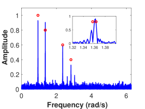
(a) 1bPER

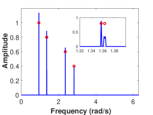
(b) ADMM

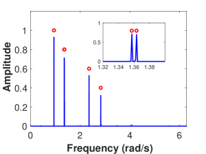
(c) 1bSPICE

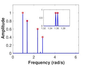
(d) 1bLIKES

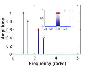
(e) 1bSLIM

(f) 1bIAA

Figure 2: Spectra obtained via (a) 1bPER, (b) ADMM, (c) 1bSPICE, (d) 1bLIKES, (e) 1bSLIM, (f) 1bIAA. The circles in the plots indicate the true values of the amplitudes.

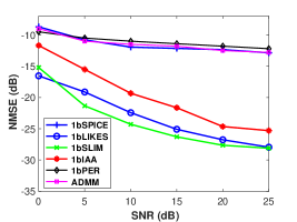
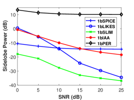
Figure 3: Estimation performance of 1bPER, ADMM, 1bSPICE, 1bLIKES, 1bSLIM and 1bIAA (from 500 Monte Carlo runs): (a) average NMSEs versus SNR, (b) average sidelobe power versus SNR.

To further illustrate the performance of the algorithms, we show the average NMSEs of the amplitude estimates as well as the average sidelobe powers, obtained from 500 Monte Carlo runs, as functions of SNR in Fig. 3 and Fig. 3. The average NMSE and sidelobe power $P_{\rm s}$ are calculated as:

$${\rm NMSE}=\frac{1}{2500}\sum_{k=1}^{5}\sum_{i=1}^{500}\frac{|\hat{\alpha}_{k}^{(i)}-\alpha_{k}|^{2}}{\alpha_{k}^{2}},$$

$$P_{\rm s}=\frac{1}{500}\sum_{i=1}^{500}\left(\|\hat{\boldsymbol{\gamma}}^{(i)}\|^{2}-\sum_{k=1}^{5}\left(\hat{\alpha}^{(i)}_{k}\right)^{2}\right),$$

where $\hat{\alpha}_{k}^{(i)}$ denotes the estimate of $\alpha_{k}$ in the $i$th Monte Carlo run; $\hat{\boldsymbol{\gamma}}^{(i)}$ represents the estimated sparse parameter vector in the $i$th Monte Carlo run and each Monte Carlo run corresponds to an independent noise and threshold realization. Inspecting the results, we see that 1bPER gives poor amplitude estimates and high sidelobe levels. Furthermore, as the SNR increases, there is little improvement in its amplitude estimation accuracy and sidelobe levels. The ADMM approach provides slightly better results than 1bPER. Since ADMM provides a very sparse spectrum, we do not plot its sidelobe power. 1bSPICE provides competitive sidelobe levels, but its amplitude estimates are biased downward. 1bLIKES and 1bSLIM have similar amplitude estimation performances, and 1bSLIM has lower sidelobe levels at low SNRs. In this example, 1bIAA performs slightly worse than 1bSLIM and 1bLIKES in terms of both amplitude estimation accuracy and sidelobe levels.

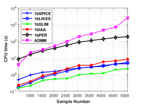
Figure 4: Average computation time versus the sample number for 1bPER, ADMM, 1bSPICE, 1bLIKES, 1bSLIM and 1bIAA for SNR=20 dB.

The average computation times needed by the aforementioned algorithms are plotted on a logarithmic scale in Fig. 4 versus the sample number $N$ and for a number of grid points $M$ equal to $5N$. The fast implementations of 1bSPICE and 1bSLIM use the CGLS approach with FFT. The fast implementations of 1bLIKES and 1bIAA make use of the Gohberg–Semencul factorization as in [29]. Note that all four proposed algorithms are more than an order of magnitude faster than the 1bPER and ADMM algorithms. Among the proposed algorithms, 1bSLIM is faster than the other three algorithms, which is due to the lower computational complexity of each iteration of 1bSLIM as well as its faster convergence speed. 1bSLIM can converge within 30 iterations, whereas the other algorithms tend to require more iterations. 1bSPICE and 1bLIKES have similar computation times, while 1bIAA tends to be slower than the other algorithms as the sample number $N$ increases.

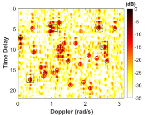
(a) 1bPER

(b) ADMM

(c) 1bSPICE

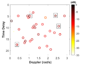
(d) 1bLIKES

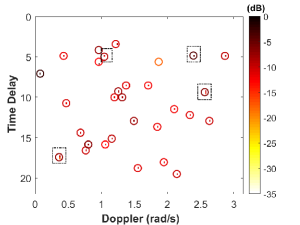
(e) 1bSLIM

(f) 1bIAA

Figure 5: The range-Doppler images of the one-bit PMCW radar for $N_{1}=31$, $N_{2}=64$, $K_{r}=4N_{1}$, $K_{d}=5N_{2}$, and SNR=15 dB. (a) 1bPER, (b) ADMM, (c) 1bSPICE, (d) 1bLIKES, (e) 1bSLIM, (f) 1bIAA. “$\bigcirc$” indicates the locations of the true targets (color-coded according to power, in dB). The dash-dot rectangles indicate the off-grid targets.

VI-A2 Range-Doppler imaging for PMCW radar

For the PMCW radar, we use a maximum length sequence (m-sequence) with length $N_{1}=31$ and $N_{2}=64$ periods within a CPI as the probing waveform. The number of grid points in the range and Doppler domains are set to $K_{\rm r}=4N_{1}$, $K_{\rm d}=5N_{2}$, respectively. The scene of interest consists of 30 targets, with their range-Doppler locations and powers indicated by the color-coded ‘$\bigcirc$’ in Fig. 5. Note that there are four off-grid targets marked with dash-dot rectangles. The amplitudes of the targets $\{\alpha_{k}\}_{k=1}^{30}$ are selected randomly between 0.1 and 1. In practical applications, the time-varying threshold can be generated by a low-rate and low-precision DAC. To reduce the sampling rate of the DAC for cost reasons, we use a PRI-varying threshold, that is the threshold is constant within each PRI and only changes from one PRI to another. The real and imaginary parts of the PRI-varying threshold are selected randomly and equally likely from a predefined eight-element set $\{-h_{\max},-h_{\max}+\Delta,\dots,h_{\max}-\Delta,h_{\max}\}$ with $h_{\max}=\frac{\sqrt{\sum_{k=1}^{30}{\alpha_{k}^{2}}+\sigma^{2}}}{2}$ and $\Delta=\frac{2h_{\max}}{7}$. The SNR, which is defined as $10\log_{10}\frac{\sum_{k=1}^{30}\alpha_{k}^{2}}{\sigma^{2}}$, is set to 15 dB.

The range-Doppler imaging result obtained by using 1bPER with the one-bit data is shown in Fig. 5(a). As expected, 1bPER suffers from high sidelobe problems. As a result, the weak targets are buried in the sidelobes of strong targets. In Fig. 5(b), we show the result of the ADMM approach [15]. ADMM misses quite a few weak targets. The range-Doppler image of 1bSPICE is shown in Fig. 5(c). 1bSPICE misses one weak target, but provides much lower sidelobe levels than 1bPER and more accurate target estimates than ADMM.

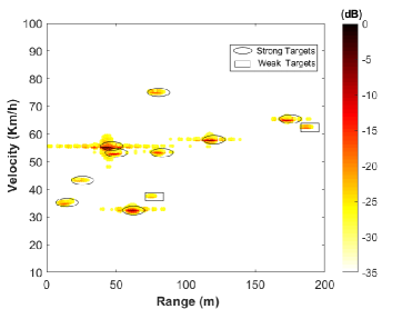
(a) 2-D FFT

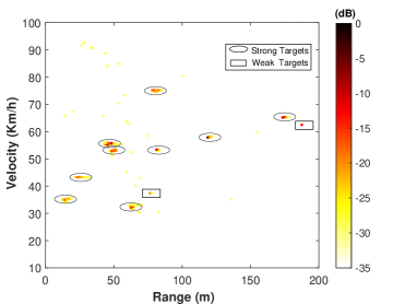
(b) The conventional IAA

Figure 6: Range-Doppler images of LFMCW radar, obtained applying (a) 2-D FFT and (b) the conventional IAA, to the original high-precision measured data.

In the 1bLIKES image, shown in Fig. 5(d), the location and power of each target are accurately estimated. In Fig. 5(e), we show the range-Doppler image of 1bSLIM. 1bSLIM misses two weak targets basically because the 1bSLIM image is too sparse. Finally, 1bIAA, as shown in Fig. 5(f), provides accurate range-Doppler imaging results and identifies all targets in the scene. Furthermore, 1bLIKES has noticeably more relatively strong spurious peaks (clearly visible when viewed in color) than 1bIAA, making 1bIAA the best method for this example.

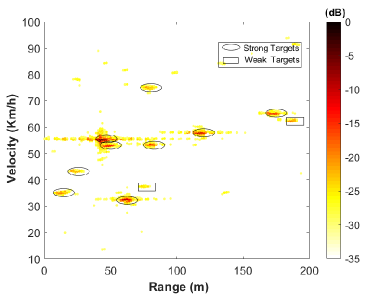
(a) 1bPER

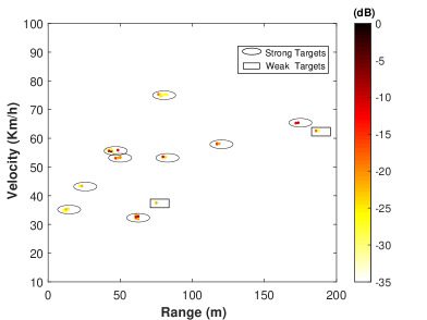
(b) 1bSPICE

(c) 1bLIKES

(d) 1bSLIM

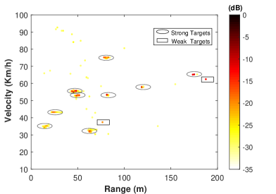
(e) 1bIAA

Figure 7: Range-Doppler images of one-bit LFMCW radar, obtained applying (a) 1bPER, (b) 1bSPICE, (c) 1bLIKES, (d) 1bSLIM, (e) 1bIAA, to the one-bit measured data.

VI-B Experimental Example

In this section, we present an experimental example to demonstrate the performance of the proposed one-bit weighted SPICE algorithms for range-Doppler imaging via a one-bit LFMCW radar. The experimental data is collected using a 24 GHz radar sensor with bandwidth 25 MHz and PRI 80 ${\rm\mu s}$. The received signal is sampled by 16-bit ADCs and the samples contain additive noise with unknown variance. The dimensions of the 2-D data matrix are $N_{1}=64$ (for range) and $N_{2}=512$ (for Doppler). The number of grid points in the range and Doppler domains are set to $K_{\rm r}=4N_{1}$, $K_{\rm d}=4N_{2}$, respectively. Similar to the PMCW case in the previous example, we use a PRI-varying threshold scheme that keeps the threshold constant within each chirp and only changes the threshold from chirp to chirp. Assume $A$ is the signal power in the high-precision data. Again, in practical systems, a rough estimate of the received signal power can be obtained from an AGC circuit. The one-bit data is obtained comparing the high-precision data with a PRI-varying threshold whose real and imaginary parts are randomly selected from an eight-element set $\{-h_{\max},-h_{\max}+\Delta,\dots,h_{\max}-\Delta,h_{\max}\}$ with $h_{\max}=\frac{\sqrt{A}}{2}$ and $\Delta=\frac{2h_{\max}}{7}$.
In Figs. 6(a) and 6(b), we show the benchmark range-Doppler images obtained by 2-D FFT and the conventional IAA applied to the high-precision data. Note that 9 strong targets and 2 weak targets are visible in both 2-D FFT and IAA images. In addition, a superposition of multiple point scatterers is identified by the radar as a single target. Compared with 2-D FFT, IAA drastically reduces the sidelobe levels and improves the resolution. For the present data size, the memory needed by the ADMM approach exceeds the maximum size limit of MATLAB, and hence ADMM is not considered in this comparison. Fig. 7(a) shows the range-Doppler image obtained by applying 1bPER to the one-bit data. Note that 1bPER smears the targets significantly and generates significant background clutter. Figs. 7(b)–7(e) show the range-Doppler imaging results obtained by the one-bit weighted SPICE algorithms applied to the one-bit data. All strong targets are accurately estimated and the two weak targets are detected reasonably well by the proposed algorithms. Interestingly, the result of 1bIAA using one-bit data is quite similar to that of the conventional IAA using high-precision data. Furthermore, the proposed one-bit weighted SPICE algorithms applied to one-bit data outperforms the 2-D FFT approach applied to the high-precision data in terms of sidelobe levels and resolution, thereby demonstrating the effectiveness of the algorithms proposed in this paper.

VII Conclusions

We have considered range-Doppler imaging via one-bit automotive LFMCW/PMCW radar systems, which use one-bit sampling with time-varying thresholds at the receiver to obtain signed measurements. We have formulated the range-Doppler imaging problem as one-bit sparse-parameter estimation. We have first presented a user parameter-free regularized minimization approach, namely 1bSLIM, to obtain accurate range-Doppler estimates. Inspired by the relationship between 1bSLIM and the original SLIM for high-precision data, we have also extended the conventional SPICE, LIKES and IAA to the one-bit data case, referred to as 1bSPICE, 1bLIKES and 1bIAA. These four hyperparameter-free algorithms have been unified under the one-bit weighted SPICE umbrella. Computationally efficient implementations of the algorithms have been investigated as well. Finally, in the simulated and experimental examples, we have compared the performance of the one-bit weighted SPICE algorithms to that of the one-bit periodogram and the ADMM log-norm approach and we have shown that the proposed one-bit weighted SPICE methods are not only more accurate but also much faster.

Appendix A Majorization-Minimization Approach

MM is a type of iterative technique, which can transform a difficult optimization problem into a sequence of simpler ones [34, 33, 35, 31, 32]. Consider the following optimization problem:

$$\mathop{\rm{minimize}}\limits_{\boldsymbol{x}}f(\boldsymbol{x}).$$ (80)

For a given feasible initialization $\hat{\boldsymbol{x}}^{0}$, an MM algorithm for solving (80) is composed of two steps at the $t$th iteration: the majorization step and the minimization step. The majorization step is to find a function $g(\boldsymbol{x}|\hat{\boldsymbol{x}}^{t})$ that satisfies the following properties:

$$g(\hat{\boldsymbol{x}}^{t}|\hat{\boldsymbol{x}}^{t}) =f(\hat{\boldsymbol{x}}^{t}),$$ (81)

$$g(\boldsymbol{x}|\hat{\boldsymbol{x}}^{t}) \geq f(\boldsymbol{x}),$$ (82)

where $\hat{\boldsymbol{x}}^{t}$ is the estimate of $\boldsymbol{x}$ at the $t$th iteration. The minimization of $g(\boldsymbol{x}|\hat{\boldsymbol{x}}^{t})$, which is referred to as a majorizing function, should be easier than that of $f(\boldsymbol{x})$. The minimization step is to update $\boldsymbol{x}$ via the minimization of $g(\boldsymbol{x}|\hat{\boldsymbol{x}}^{t})$:

$$\hat{\boldsymbol{x}}^{(t+1)}=\arg\mathop{\min}_{\boldsymbol{x}}g(\boldsymbol{x}|\hat{\boldsymbol{x}}^{t}).$$ (83)

The objective function $f(\boldsymbol{x})$ is guaranteed to decrease monotonically at each MM iteration because:

$$f(\hat{\boldsymbol{x}}^{t})=g(\hat{\boldsymbol{x}}^{t}|\hat{\boldsymbol{x}}^{t})\geq g(\hat{\boldsymbol{x}}^{(t+1)}|\hat{\boldsymbol{x}}^{t})\geq f(\hat{\boldsymbol{x}}^{(t+1)}).$$ (84)

Appendix B Proof of the Inequality (25)

Assume $\boldsymbol{P}\succ 0$. Then, we have the inequality

$$\boldsymbol{D} =\left[\begin{matrix}(\hat{\boldsymbol{R}}^{t})^{-1}\vec{A}\hat{\boldsymbol{P}}^{t}\vec{P}^{-1}\hat{\boldsymbol{P}}^{t}\boldsymbol{A}^{H}(\hat{\boldsymbol{R}}^{t})^{-1}&\boldsymbol{I}\\ \boldsymbol{I}&\boldsymbol{R}\end{matrix}\right]$$

$$=\left[\begin{matrix}(\hat{\boldsymbol{R}}^{t})^{-1}\boldsymbol{A}\hat{\boldsymbol{P}}^{t}\boldsymbol{P}^{-\frac{1}{2}}\\ \boldsymbol{A}\boldsymbol{P}^{\frac{1}{2}}\end{matrix}\right]\left[\begin{matrix}\boldsymbol{P}^{-\frac{1}{2}}\hat{\boldsymbol{P}}^{t}\boldsymbol{A}^{H}(\hat{\boldsymbol{R}}^{t})^{-1}&\boldsymbol{P}^{\frac{1}{2}}\boldsymbol{A}^{H}\end{matrix}\right]\succeq 0.$$ (85)

By the properties of the Schur complement of $\boldsymbol{R}$ in $\boldsymbol{D}$, $\boldsymbol{D}\succeq 0$ implies

$$\vec{R}^{-1}\preceq(\hat{\boldsymbol{R}}^{t})^{-1}\vec{A}\hat{\boldsymbol{P}}^{t}\vec{P}^{-1}\hat{\boldsymbol{P}}^{t}\boldsymbol{A}^{H}(\hat{\boldsymbol{R}}^{t})^{-1}.$$ (86)

References

- [1] F. Meinl, M. Stolz, M. Kunert, and H. Blume, “An experimental high performance radar system for highly automated driving,” in Proc. IEEE MTT-S Int. Conf. on Microwaves for Intelligent Mobility, Nagoya, Japan, March 2017.
- [2] I. Bilik, O. Longman, S. Villeval, and J. Tabrikian, “The rise of radar for autonomous vehicles: Signal processing solutions and future research directions,” IEEE Signal Process. Mag., vol. 36, no. 5, pp. 20–31, 2019.
- [3] S. M. Patole, M. Torlak, D. Wang, and M. Ali, “Automotive radars: A review of signal processing techniques,” IEEE Signal Process. Mag., vol. 34, no. 2, pp. 22–35, 2017.
- [4] F. Engels, P. Heidenreich, A. M. Zoubir, F. K. Jondral, and M. Wintermantel, “Advances in automotive radar: A framework on computationally efficient high-resolution frequency estimation,” IEEE Signal Process. Mag., vol. 34, no. 2, pp. 36–46, 2017.
- [5] R. Lin, M. Soltanalian, B. Tang, and J. Li, “Efficient design of binary sequences with low autocorrelation sidelobes,” IEEE Trans. Signal Process., vol. 67, no. 24, pp. 6397–6410, 2019.
- [6] S. Alland, W. Stark, M. Ali, and M. Hegde, “Interference in automotive radar systems: Characteristics, mitigation techniques, and current and future research,” IEEE Signal Process. Mag., vol. 36, no. 5, pp. 45–59, 2019.
- [7] J. Li and P. Stoica, MIMO radar signal processing. Wiley, 2009.
- [8] A. E. Ertan and M. Ali, “Spatial and temporal smoothing for covariance estimation in super-resolution angle estimation in automotive radars,” in Proc. IEEE Int. Conf. Acoust. Speech Signal Process., Barcelona, Spain, May 2020.
- [9] G. Hakobyan and B. Yang, “High-performance automotive radar: A review of signal processing algorithms and modulation schemes,” IEEE Signal Process. Mag., vol. 36, no. 5, pp. 32–44, 2019.
- [10] V. Giannini, D. Guermandi, Q. Shi, A. Medra, W. Van Thillo, A. Bourdoux, and P. Wambacq, “A 79 GHz phase-modulated 4 GHz-BW CW radar transmitter in 28 nm CMOS,” IEEE J. Solid-State Circuits, vol. 49, no. 12, pp. 2925–2937, 2014.
- [11] R. Zhang, C. Li, J. Li, and G. Wang, “Range estimation and range-Doppler imaging using signed measurements in LFMCW radar,” IEEE Trans. Aerosp. Electron. Syst., vol. 55, no. 6, pp. 3531–3550, 2019.
- [12] B. Zhao, L. Huang, and W. Bao, “One-bit SAR imaging based on single-frequency thresholds,” IEEE Trans. Geosci. Remote Sens., vol. 57, no. 9, pp. 7017–7032, 2019.
- [13] F. Li, J. Fang, H. Li, and L. Huang, “Robust one-bit Bayesian compressed sensing with sign-flip errors,” IEEE Signal Process. Lett., vol. 22, no. 7, pp. 857–861, 2014.
- [14] A. Host-Madsen and P. Handel, “Effects of sampling and quantization on single-tone frequency estimation,” IEEE Trans. Signal Process., vol. 48, no. 3, pp. 650–662, 2000.
- [15] H. Zhu, F. Liu, and J. Li, “Computationally efficient sinusoidal parameter estimation from signed measurements: ADMM approaches,” IEEE Signal Process. Lett., vol. 26, no. 12, pp. 1798–1802, 2019.
- [16] Y. Li, C. Tao, G. Seco-Granados, A. Mezghani, A. L. Swindlehurst, and L. Liu, “Channel estimation and performance analysis of one-bit massive MIMO systems,” IEEE Trans. Signal Process., vol. 65, no. 15, pp. 4075–4089, 2017.
- [17] J. Choi, J. Mo, and R. W. Heath, “Near maximum-likelihood detector and channel estimator for uplink multiuser massive MIMO systems with one-bit ADCs,” IEEE Trans. Commun., vol. 64, no. 5, pp. 2005–2018, 2016.
- [18] J. Mo, P. Schniter, and R. W. Heath, “Channel estimation in broadband millimeter wave MIMO systems with few-bit ADCs,” IEEE Trans. Signal Process., vol. 66, no. 5, pp. 1141–1154, 2017.
- [19] O. Bar-Shalom and A. J. Weiss, “DOA estimation using one-bit quantized measurements,” IEEE Trans. Aerosp. Electron. Syst., vol. 38, no. 3, pp. 868–884, 2002.
- [20] M. Yan, Y. Yang, and S. Osher, “Robust 1-bit compressive sensing using adaptive outlier pursuit,” IEEE Trans. Signal Process., vol. 60, no. 7, pp. 3868–3875, 2012.
- [21] K. Knudson, R. Saab, and R. Ward, “One-bit compressive sensing with norm estimation,” IEEE Trans. Inf. Theory, vol. 62, no. 5, pp. 2748–2758, 2016.
- [22] J. Ren, T. Zhang, J. Li, and P. Stoica, “Sinusoidal parameter estimation from signed measurements via majorization–minimization based RELAX,” IEEE Trans. Signal Process., vol. 67, no. 8, pp. 2173–2186, 2019.
- [23] P. Stoica, D. Zachariah, and J. Li, “Weighted SPICE: A unifying approach for hyperparameter-free sparse estimation,” Digital Signal Processing, vol. 33, pp. 1–12, 2014.
- [24] P. Stoica, P. Babu, and J. Li, “New method of sparse parameter estimation in separable models and its use for spectral analysis of irregularly sampled data,” IEEE Trans. Signal Process., vol. 59, no. 1, pp. 35–47, 2010.
- [25] P. Stoica and P. Babu, “SPICE and LIKES: Two hyperparameter-free methods for sparse-parameter estimation,” Signal Process., vol. 92, no. 7, pp. 1580–1590, 2012.
- [26] X. Tan, W. Roberts, J. Li, and P. Stoica, “Sparse learning via iterative minimization with application to MIMO radar imaging,” IEEE Trans. Signal Process., vol. 59, no. 3, pp. 1088–1101, 2010.
- [27] T. Yardibi, J. Li, P. Stoica, M. Xue, and A. B. Baggeroer, “Source localization and sensing: A nonparametric iterative adaptive approach based on weighted least squares,” IEEE Trans. Aerosp. Electron. Syst., vol. 46, no. 1, pp. 425–443, 2010.
- [28] W. Roberts, P. Stoica, J. Li, T. Yardibi, and F. A. Sadjadi, “Iterative adaptive approaches to MIMO radar imaging,” IEEE J. Sel. Topics Signal Process., vol. 4, no. 1, pp. 5–20, 2010.
- [29] M. Xue, L. Xu, and J. Li, “IAA spectral estimation: Fast implementation using the Gohberg–Semencul factorization,” IEEE Trans. Signal Process., vol. 59, no. 7, pp. 3251–3261, 2011.
- [30] S. Sun, A. P. Petropulu, and H. V. Poor, “MIMO radar for advanced driver-assistance systems and autonomous driving: Advantages and challenges,” IEEE Signal Process. Mag., vol. 37, no. 4, pp. 98–117, 2020.
- [31] M. Hong, M. Razaviyayn, Z.-Q. Luo, and J.-S. Pang, “A unified algorithmic framework for block-structured optimization involving big data: With applications in machine learning and signal processing,” IEEE Signal Process. Mag., vol. 33, no. 1, pp. 57–77, 2015.
- [32] Y. Sun, P. Babu, and D. P. Palomar, “Majorization-minimization algorithms in signal processing, communications, and machine learning,” IEEE Trans. Signal Process., vol. 65, no. 3, pp. 794–816, 2016.
- [33] P. Stoica and Y. Selen, “Cyclic minimizers, majorization techniques, and the expectation-maximization algorithm: A refresher,” IEEE Signal Process. Mag., vol. 21, no. 1, pp. 112–114, 2004.
- [34] D. R. Hunter and K. Lange, “A tutorial on MM algorithms,” The American Statistician, vol. 58, no. 1, pp. 30–37, 2004.
- [35] J. Mairal, “Incremental majorization-minimization optimization with application to large-scale machine learning,” SIAM J. Optim., vol. 25, no. 2, pp. 829–855, 2015.
- [36] Y. Sun, P. Babu, and D. P. Palomar, “Robust estimation of structured covariance matrix for heavy-tailed elliptical distributions,” IEEE Trans. Signal Process., vol. 64, no. 14, pp. 3576–3590, 2016.
- [37] S. M. Kay, Fundamentals of statistical signal processing. Prentice Hall PTR, 1993.
- [38] C. Gianelli, L. Xu, J. Li, and P. Stoica, “One-bit compressive sampling with time-varying thresholds: Maximum likelihood and the Cramér-Rao bound,” in Proc. 50th Asilomar Conf. Signals, Syst. Comput., Pacific Grove, USA, Nov. 2016.
- [39] A. Gelman, J. B. Carlin, H. S. Stern, D. B. Dunson, A. Vehtari, and D. B. Rubin, Bayesian data analysis. CRC press, 2013.
- [40] J. W. Daniel, “The conjugate gradient method for linear and nonlinear operator equations,” SIAM J. Numer. Anal., vol. 4, no. 1, pp. 10–26, 1967.
- [41] H. Akaike, “Block Toeplitz matrix inversion,” SIAM J. Appl. Math., vol. 24, no. 2, pp. 234–241, 1973.
- [42] P. Stoica and R. L. Moses, Spectral Analysis of Signals. Upper Saddle River, NJ: Prentice-Hall, 2005.
- [43] C. Gianelli, L. Xu, J. Li, and P. Stoica, “One-bit compressive sampling with time-varying thresholds for multiple sinusoids,” in Proc. 7th Int. Workshop Comput. Adv. Multi-Sensor Adaptive Process. (CAMSAP), Curacao, Netherlands Antilles, Mar. 2017.