Linear and nonlinear substructured Restricted Additive Schwarz iterations and preconditioning

Abstract

Substructured domain decomposition (DD) methods have been extensively studied, and they are usually associated with nonoverlapping decompositions. We introduce here a substructured version of Restricted Additive Schwarz (RAS) which we call SRAS, and we discuss its advantages compared to the standard volume formulation of the Schwarz method when they are used both as iterative solvers and preconditioners for a Krylov method. To extend SRAS to nonlinear problems, we introduce SRASPEN (Substructured Restricted Additive Schwarz Preconditioned Exact Newton), where SRAS is used as a preconditioner for Newton’s method. We study carefully the impact of substructuring on the convergence and performance of these methods as well as their implementations. We finally introduce two-level versions of nonlinear SRAS and SRASPEN. Numerical experiments confirm the advantages of formulating a Schwarz method at the substructured level.

65N55, 65F08, 65F10, 65Y05

1 Introduction

We consider a boundary value problem posed in a Lipschitz domain $\Omega\subset\mathbb{R}^{d}$, $d\in\left\{1,2,3\right\}$,

(1) $$\mathcal{L}(u) =f,\quad\text{in }\Omega,$$

$$u =0,\quad\text{on }\partial\Omega.$$

We assume that (1) admits a unique solution in some Hilbert space $\mathcal{V}$. If the boundary value problem is linear, a discretization of (1) with $N_{v}$ degrees of freedom leads to a linear system

(2) $$A\mathbf{u}=\mathbf{f},$$

where $A\in\mathbb{R}^{N_{v}\times N_{v}}$, $\mathbf{u}\in V(\cong\mathbb{R}^{N_{v}})$, and $\mathbf{f}\in V$. If the boundary value problem is nonlinear, we obtain a nonlinear system

(3) $$F(\mathbf{u})=0,$$

where $F:V\rightarrow V$ is a nonlinear function and $\mathbf{u}\in V$. Several numerical methods have been proposed in the last decades for the efficient solution of such boundary value problems, e.g., multigrid methods [23, 36] and domain decomposition (DD) methods [35, 33]. We will focus on DD methods, which are usually divided into two distinct classes, that is overlapping methods, which include the AS (Additive Schwarz) and RAS (Restricted Additive Schwarz) methods [35, 6], and nonoverlapping methods such as FETI (Finite Element Tearing and Interconnect) and Neumann-Neumann methods [16, 31, 26]. Concerning nonlinear problems, DD methods can be applied either as nonlinear iterative methods, that is by just solving nonlinear problems in each subdomain and then exchanging information between subdomains as in the linear case [28, 29, 2], or as preconditioners to solve the Jacobian linear system inside Newton iteration. In the latter case, the term Newton-Krylov-DD is employed, where DD is replaced by the domain decomposition preconditioner used [24].

An alternative is to use a DD method as a preconditioner for Newton’s method. Preconditioning a nonlinear system $F(\mathbf{u})=0$ means that we aim to replace the original nonlinear system with a new nonlinear system, still having the same solution, but for which the nonlinearities are more balanced and Newton’s method converges faster [3, 19]. Seminal contributions in nonlinear preconditioning have been made by Cai and Keyes in [3, 4], where they introduced ASPIN (Additive Schwarz Preconditioned Inexact Newton), which is a left preconditioner. Extensions of this idea to Dirichlet-Neumann, FETI-DP and BDDC are presented in [7, 25]. The development of good preconditioners is not an easy task even in the linear case. One useful strategy is to study efficient iterative methods, and then to use the associated preconditioners in combination with Krylov methods [19]. The same logical path paved the way to the development of RASPEN (Restricted Additive Schwarz Preconditioned Exact Newton) in [15], which in short applies Newton’s method to the fixed point equation defined by the nonlinear RAS iteration at convergence. All these methods are left preconditioners. Right preconditioners are usually based on the concept of nonlinear elimination, presented in [27], and they are very efficient as shown in [22, 21, 5, 30]. While left preconditioners aim to transform the original nonlinear function into a better behaved one, right preconditioners aim to provide a better initial guess for the next outer Newton iteration.

Nonoverlapping methods are sometimes called substructuring methods (a term borrowed from Przemieniecki’s work [32]), as in these methods the unknowns in the interior of the nonoverlapping domains are eliminated through static condensation so that one needs to solve a smaller system involving only the degrees of freedom on the interfaces between the nonoverlapping subdomains, like in the more recent hybridizable discontinuous Galerkin finite element methods, where each element forms a subdomain [13]. However, it is also possible to write an overlapping method, such as Lions’ Parallel Schwarz Method (PSM), which is equivalent to RAS [18], in substructured form, even though this approach is much less common in the literature. For a two subdomain decomposition, a substructuring procedure applied to the PSM is carried out in [17, Section 5], [20, Section 3.4] and [10], while for a many subdomain decomposition with cross-points we refer to [12, 11]. In this particular framework, the substructured unknowns are now the degrees of freedom located on the portions of a subdomain boundary that lie in the interior of another subdomain; that is where the overlapping DD method takes the information to compute the new iterate. We emphasize that, at a given iteration $n$, any iterative DD method (overlapping or nonoverlapping) needs only a few values of $\mathbf{u}^{n}$ to compute the new approximation $\mathbf{u}^{n+1}$. The major part of $\mathbf{u}^{n}$ is useless.

In this manuscript, we define a substructured version of RAS, that is we define an iterative scheme based on RAS which acts only over unknowns that are located on the portions of a subdomain boundary that lie in the interior of another subdomain. We study in detail the effects that such a substructuring procedure has on RAS when the latter is applied either as an iterative solver or as a preconditioner to solve linear and nonlinear boundary value problems. Does the substructured iterative version converge faster than the volume one? Is the convergence of GMRES affected by substructuring? What about nonlinear problems when instead of preconditioned GMRES we rely on preconditioned Newton? We prove that substructuring does not influence the convergence of the iterative methods both in the linear and nonlinear case, by showing that at each iteration, the restriction on the interfaces of the volume iterates coincides with the iterates of the substructured iterative method. This equivalence of iterates does not hold anymore when considering preconditioned GMRES. Specifically, our study shows that GMRES should always be applied to the substructured system, since it is computationally less expensive, requiring to perform orthogonalization on a much smaller space, and thus needs also less memory. In contrast to the linear case, we prove that the nonlinear preconditioners RASPEN and SRASPEN (Substructured RASPEN) for Newton produce the same iterates once these are restricted to the interfaces. However, SRASPEN has again more favorable properties when assembling and solving the Jacobian matrices at each Newton iteration. Finally, we also extend the work in [12, 10, 11] defining substructured two-level methods to the nonlinear case, where both smoother and coarse correction are defined directly on the interfaces between subdomains.

This paper is organized as follows: we introduce in Section 2 the mathematical setting with the domain, subdomains and operators defined on them. In Section 3, devoted to the linear case, we study the effects of substructuring on RAS and on GMRES applied to the preconditioned system. In Section 4, we extend our analysis to nonlinear boundary value problems. Section 5 contains two-level substructured methods for the nonlinear problems. Finally Section 6 provides extensive numerical tests to corroborate the framework proposed.

2 Notation

Let us decompose the domain $\Omega$ into $N$ nonoverlapping subdomains $\Omega_{j}$, that is $\Omega=\bigcup_{j\in\mathcal{J}}\Omega_{j}$ with $\mathcal{J}:=\{1,2,\dots,N\}$.

Figure 1: The domain $\Omega$ is divided into nine nonoverlapping subdomains (left). The center panel shows how the diagonal nonoverlapping subdomains are enlarged to form overlapping subdomains. On the right, we denote the unknowns represented in $\overline{V}$ (blue line) and the unknowns of a coarse space of $\overline{V}$ (red crosses).

The nonoverlapping subdomains $\Omega_{j}$ are then enlarged to obtain subdomains $\Omega^{\prime}_{j}$ which form an overlapping decomposition of $\Omega$. For each subdomain $\Omega^{\prime}_{j}$, we define $V_{j}$ as the restriction of $V$ to $\Omega^{\prime}_{j}$, that is $V_{j}$ collects the degrees of freedom on $\Omega^{\prime}_{j}$. Further, we introduce the classical restriction and prolongation operators $R_{j}:V\rightarrow V_{j}$, $P_{j}:V_{j}\rightarrow V$, and the restricted prolongation operators $\widetilde{P}_{j}:V_{j}\rightarrow V$. We assume that these operators satisfy

(4) $$R_{j}P_{j}=I_{V_{j}},\quad\mbox{and}\quad\sum_{j\in\mathcal{J}}\widetilde{P}_{j}R_{j}=I,$$

where $I_{V_{j}}$ is the identity on $V_{j}$ and $I$ is the identity on $V$.

We now define the substructured skeleton. In the following, we use the notation introduced in [9]. For any $j\in\mathcal{J}$, we define the set of neighboring indices $N_{j}:=\{\ell\in\mathcal{J}\,:\,\Omega^{\prime}_{j}\cap\partial\Omega^{\prime}_{\ell}\neq\emptyset\}$. Given a $j\in\mathcal{J}$, we introduce the substructure of $\Omega^{\prime}_{j}$ defined as $S_{j}:=\bigcup_{\ell\in N_{j}}\bigl{(}\partial\Omega^{\prime}_{\ell}\cap\Omega^{\prime}_{j}\bigr{)}$, that is the union of all the portions of $\partial\Omega^{\prime}_{\ell}$ with $\ell\in N_{j}$. The substructure of the whole domain $\Omega$ is defined as $S:=\bigcup_{j\in\mathcal{I}}\overline{S_{j}}$. A graphical representation of $S$ is given in Figure 1 for a decomposition of a square into nine subdomains. We now introduce the space $\overline{V}$ as the trace space of $V$ onto the substructure $S$, i.e. $\overline{V}$ collects the $\overline{N}$ degrees of freedom which lie on $S$. Associated to $\overline{V}$, we consider the restriction operator $\overline{R}:V\rightarrow\overline{V}$ and a prolongation operator $\overline{P}:\overline{V}\rightarrow V$. The restriction operator $\overline{R}$ takes an element $v\in V$ and restricts it to the skeleton $S$. The prolongation operator $\overline{P}$ extends an element $v\in\overline{V}$ to the global space $V$. In our numerical experiments, $\overline{P}$ extends an element $v_{S}\in\overline{V}$ by zero in $\Omega\setminus S$. However, we can consider several different prolongation operators. How this extension is done is not crucial as we will use $\overline{P}$ inside a domain decomposition algorithm, and thus only the values on the skeleton $S$ will play a role. Hence, as of now, we will need only one assumption on the restriction and prolongation operator, namely

(5) $$\overline{R}\overline{P}=\overline{I},$$

where $\overline{I}$ is the identity over $\overline{V}$.

3 The linear case

In this section, we focus on the linear problem $A\mathbf{u}=\mathbf{f}$. After defining a substructured variant of RAS called SRAS, we prove the equivalence between RAS and SRAS. Then, we study in detail how GMRES performs if applied to the volume preconditioned system or the substructured system.

3.1 Linear iterative methods

To introduce our analysis, we recall the classical definition of RAS to solve the linear system (2). RAS starts from an approximation $\mathbf{u}^{0}$ and computes for $n=1,2,\dots$,

(6) $$\mathbf{u}^{n}=\mathbf{u}^{n-1}+\sum_{j\in\mathcal{J}}\widetilde{P}_{j}A^{-1}_{j}R_{j}\left(\mathbf{f}-A\mathbf{u}^{n-1}\right),$$

where $A_{j}:=R_{j}AP_{j}$, that is, we use exact local solvers. Let us now rewrite the iteration (6) in an equivalent form using the hypothesis in (4) and the definition of $A_{j}$,

(7) $$\mathbf{u}^{n} = \sum_{j\in\mathcal{J}}\widetilde{P}_{j}R_{j}\mathbf{u}^{n-1}+\sum_{j\in\mathcal{J}}\widetilde{P}_{j}A^{-1}_{j}R_{j}\left(\mathbf{f}-A\mathbf{u}^{n-1}\right)$$

$$= \sum_{j\in\mathcal{J}}\widetilde{P}_{j}A^{-1}_{j}\left(A_{j}R_{j}\mathbf{u}^{n-1}+R_{j}\left(\mathbf{f}-A\mathbf{u}^{n-1}\right)\right)$$

$$= \sum_{j\in\mathcal{J}}\widetilde{P}_{j}A^{-1}_{j}R_{j}\left(\mathbf{f}-A\left(I-P_{j}R_{j}\right)\mathbf{u}^{n-1}\right)$$

$$= :G^{\text{RAS}}(\mathbf{u}^{n-1}).$$

We emphasize that $\left(P_{j}R_{j}-I\right)\mathbf{u}^{n-1}$ contains non-zero elements only outside subdomain $\Omega^{\prime}_{j}$, and in particular the terms $A\left(P_{j}R_{j}-I\right)\mathbf{u}^{n-1}$ represent precisely the boundary conditions for $\Omega^{\prime}_{j}$ given the old approximation $\mathbf{u}^{n-1}$. This observation suggests that RAS, like most domain decomposition methods, can be written in substructured form. Indeed, despite iteration (7) being written in volume form, involving the entire vector $\mathbf{u}^{n-1}$, only very few elements of $\mathbf{u}^{n-1}$ are needed to compute the new approximation $\mathbf{u}^{n}$. For further details about a substructured formulation of the parallel Schwarz method at the continuous level, we refer to [20] for the two subdomain case, and [12, 10, 11] for a general decomposition into several subdomains with cross points.

In Section 2, we introduced the substructured space $\overline{V}$ geometrically, but we can also provide an algebraic characterization using the RAS operators $R_{j}$ and $P_{j}$. We consider

$$\mathcal{K}:=\left\{k\in\left\{1,\dots,N_{v}\right\}:\exists j\in\left\{1,\dots,N\right\}\text{ such that }R_{j}A(\mathbf{e}_{k}-P_{j}R_{j}\mathbf{e}_{k})\neq 0\right\},$$

that is, $\mathcal{K}$ is the set of indices such that the canonical vectors $\mathbf{e}_{k}$ represent a Dirichlet boundary condition at least for a subdomain, and its complement $\mathcal{K}^{c}:=\left\{1,\dots,N_{v}\right\}\setminus\mathcal{K}$. The cardinality of $\mathcal{K}$ is $|\mathcal{K}|=:\overline{N}$. We can thus introduce

$$\widehat{V}:=\left\{\mathbf{v}\in\mathbb{R}^{N_{v}}:\text{ if }j\notin\mathcal{K}\text{ then }v_{j}=0\right\}=\text{span}\left\{\mathbf{e}_{k}\right\}_{k\in\mathcal{K}}\subset\mathbb{R}^{N_{v}}.$$

Finally $\overline{R}$ is the Boolean restriction operator, mapping a vector of $\mathbb{R}^{N_{v}}$ onto a vector of $\mathbb{R}^{\overline{N}}$, keeping only the indices in $\mathcal{K}$. Hence, $\overline{V}:=\text{Im}\overline{R}(\cong\mathbb{R}^{\overline{N}})$ and $\overline{P}=\overline{R}^{\top}$.

To define SRAS, we need one more assumption on the restriction and prolongation operators, namely

(8) $$\overline{R}M^{-1}A=\overline{R}M^{-1}A\overline{PR},$$

where $M^{-1}$ is the preconditioner for RAS, formally defined as

(9) $$M^{-1}:=\sum_{j\in\mathcal{J}}\widetilde{P}_{j}A^{-1}_{j}R_{j}.$$

Heuristically, this assumption means that the operator $\overline{P}\overline{R}$ preserves all the information needed by $G^{\text{RAS}}$ (defined in (7)) to compute correctly the values of the new iterate on the skeleton $S$. Indeed a direct calculation shows that (8) is equivalent to the condition

$$\overline{R}G^{\text{RAS}}(\mathbf{u})=\overline{R}G^{\text{RAS}}(\overline{P}\overline{R}\mathbf{u}).$$

Given a substructured approximation $\mathbf{v}^{0}\in\overline{V}$, for $n=1,2,\dots$, we define SRAS as

(10) $$\mathbf{v}^{n}=G^{\text{SRAS}}(\mathbf{v}^{n-1}),\quad\text{where}\quad G^{\text{SRAS}}(\mathbf{v}):=\overline{R}G^{\text{RAS}}(\overline{P}\mathbf{v}).$$

RAS and SRAS are tightly linked, but when are they equivalent? Clearly, we must impose some conditions on $\overline{P}$ and $\overline{R}$. The next theorem shows that assumption (8) is in fact sufficient for equivalence.

Theorem 3.1 (Equivalence between RAS and SRAS).

Assume that the operators $\overline{R}$ and $\overline{P}$ satisfy (8). Given an initial guess $\mathbf{u}^{0}\in V$ and its substructured restriction $\mathbf{v}^{0}:=\overline{R}\mathbf{u}^{0}\in\overline{V}$, define the sequences $\left\{\mathbf{u}^{n}\right\}$ and $\left\{\mathbf{v}^{n}\right\}$ such that

$$\mathbf{u}^{n}=G^{\text{RAS}}(\mathbf{u}^{n-1}),\quad\mathbf{v}^{n}=G^{\text{SRAS}}(\mathbf{v}^{n-1}).$$

Then, $\overline{R}\mathbf{u}^{n}=\mathbf{v}^{n}$ for every iteration $n\geq 1$.

Proof 3.2.

We prove this statement for $n=1$ by a direct calculation. Taking the restriction of $\mathbf{u}^{1}$ we have

$$\overline{R}\mathbf{u}^{1}=\overline{R}G^{\text{RAS}}(\mathbf{u}^{0})=\overline{R}G^{\text{RAS}}(\overline{P}\overline{R}\mathbf{u}^{0})=\overline{R}G^{\text{RAS}}(\overline{P}\mathbf{v}^{0})=G^{\text{SRAS}}(\mathbf{v}^{0})=\mathbf{v}^{1},$$

where we used assumption (8), and the definition of $\mathbf{v}^{0}$ and $G^{\text{SRAS}}$. For a general $n$, the proof is obtained by induction.

3.2 Linear preconditioners for GMRES

It is well known that any stationary iterative method should be used in practice as a preconditioner for a Krylov method, since the Krylov method finds in general a much better residual polynomial with certain optimality properties, compared to the residual polynomial of the stationary iteration, see e.g. [8, Section 4.1]. The preconditioner associated to RAS is $M^{-1}$ and is defined in (9). The preconditioned volume system then reads

(11) $$M^{-1}A\mathbf{u}=M^{-1}\mathbf{f}.\\$$

To discover the preconditioner associated with SRAS, we consider the fixed point limit of (10),

(12) $$\mathbf{v} =G^{\text{SRAS}}(\mathbf{v})=\overline{R}G^{\text{RAS}}(\overline{P}\mathbf{v})=\overline{R}\left(\overline{P}\mathbf{v}+\sum_{j\in\mathcal{J}}\widetilde{P}_{j}A_{j}^{-1}R_{j}(\mathbf{f}-A\overline{P}\mathbf{v})\right)$$

$$=\mathbf{v}+\overline{R}\sum_{j\in\mathcal{J}}\widetilde{P}_{j}A_{j}^{-1}R_{j}\mathbf{f}-\overline{R}\sum_{j\in\mathcal{J}}\widetilde{P}_{j}A_{j}^{-1}R_{j}A\overline{P}\mathbf{v}$$

$$=\mathbf{v}+\overline{R}M^{-1}\mathbf{f}-\overline{R}M^{-1}A\overline{P}\mathbf{v},$$

where in the second line we used the identity $\overline{R}\overline{P}=I_{S}$. We can thus consider the preconditioned substructured system

(13) $$\overline{R}M^{-1}A\overline{P}\mathbf{v}=\overline{R}M^{-1}\mathbf{f}.$$

It is then natural to ask how a Krylov method like GMRES performs if applied to (11), compared to (13).

Let us consider an initial guess in volume $\mathbf{u}^{0}$, its restriction $\mathbf{v}^{0}:=\overline{R}\mathbf{u}^{0}$ and the initial residuals $\mathbf{r}^{0}:=M^{-1}(\mathbf{f}-A\mathbf{u}^{0})$, $\overline{\mathbf{r}}^{0}:=\overline{R}M^{-1}(\mathbf{f}-A\overline{P}\mathbf{v}^{0})$. Then GMRES applied to the preconditioned systems (11) and (13) looks for solutions in the affine Krylov spaces

(14) $$\mathbf{u}^{0}+\mathcal{K}_{k}(M^{-1}A,\mathbf{r}^{0}) :=\mathbf{u}^{0}+\text{ span}\left\{\mathbf{r}^{0},M^{-1}A\mathbf{r}^{0},\dots,(M^{-1}A)^{k-1}\mathbf{r}^{0}\right\}$$

$$\mathbf{v}^{0}+\mathcal{K}_{k}(\overline{R}M^{-1}A\overline{P},\overline{\mathbf{r}}^{0}) :=\mathbf{v}^{0}+\text{ span}\left\{\overline{\mathbf{r}}^{0},\overline{R}M^{-1}A\overline{P}\overline{\mathbf{r}}^{0},\dots,(\overline{R}M^{-1}A\overline{P})^{k-1}\overline{\mathbf{r}}^{0}\right\},$$

where $k\geq 1$. The two Krylov spaces are tightly linked, as Theorem 3.5 below will show. To prove it, we need the following Lemma.

Lemma 3.3.

If the restriction and prolongation operators $\overline{R}$ and $\overline{P}$ satisfy (8) then for $k\geq 1$,

(15) $$\overline{R}\left(M^{-1}A\right)^{k}=\left(\overline{R}M^{-1}A\overline{P}\right)^{k}\overline{R}.$$

Proof 3.4.

Multiplying the second equation in (8) from the right by $M^{-1}A$ we get

$$\overline{R}M^{-1}AM^{-1}A = \overline{R}M^{-1}A\overline{P}\overline{R}M^{-1}A=\overline{R}M^{-1}A\overline{P}\overline{R}M^{-1}A\overline{P}\overline{R},$$

where in the second equality we have used once more (8). Using induction, one gets for every $k\geq 1$,

$$\overline{R}\left(M^{-1}A\right)^{k}=\left(\overline{R}M^{-1}A\overline{P}\right)^{k}\overline{R},$$

and this completes the proof.

Theorem 3.5 (Relation between RAS and SRAS Krylov subspaces).

Let us consider operators $\overline{R}$ and $\overline{P}$ satisfying (8), an initial guess $\mathbf{u}^{0}\in V$, its restriction $\mathbf{v}^{0}:=\overline{R}\mathbf{u}^{0}\in\overline{V}$ and the residuals $\mathbf{r}^{0}:=M^{-1}(\mathbf{f}-A\mathbf{u}^{0})$, $\overline{\mathbf{r}}^{0}:=\overline{R}M^{-1}(\mathbf{f}-A\overline{P}\mathbf{v}^{0})$. Then for every $k\geq 1$, we have

(16) $$\mathbf{v}^{0}+\mathcal{K}_{k}(\overline{R}M^{-1}A\overline{P},\overline{\mathbf{r}}^{0})=\overline{R}(\mathbf{u}^{0}+\mathcal{K}_{k}(M^{-1}A,\mathbf{r}^{0})).$$

Proof 3.6.

First, due to (8) we have

$$\overline{R}\mathbf{r}^{0}=\overline{R}M^{-1}(\mathbf{f}-A\mathbf{u}^{0})=\overline{R}M^{-1}(\mathbf{f}-A\overline{P}\overline{R}\mathbf{u}^{0})=\overline{R}M^{-1}(\mathbf{f}-A\overline{P}\mathbf{v}^{0})=\overline{\mathbf{r}}^{0}.$$

Let us now show the first inclusion. If $\mathbf{v}\in\overline{R}\left(\mathbf{u}^{0}+\mathcal{K}_{k}(M^{-1}A,\mathbf{r}^{0})\right)$, then $\mathbf{v}=\overline{R}\mathbf{u}^{0}+\overline{R}\sum_{j=0}^{k-1}\gamma_{j}\left(M^{-1}A\right)^{j}\mathbf{r}^{0},$ for some coefficients $\gamma_{j}$. Using Lemma 3.3, we can rewrite $\mathbf{v}$ as

$$\mathbf{v} = \mathbf{v}^{0}+\sum_{j=0}^{k-1}\gamma_{j}\overline{R}\left(M^{-1}A\right)^{j}\mathbf{r}^{0}=\mathbf{v}^{0}+\sum_{j=0}^{k-1}\gamma_{j}\left(\overline{R}M^{-1}A\overline{P}\right)^{j}\overline{R}\mathbf{r}^{0}$$

$$= \mathbf{v}^{0}+\sum_{j=0}^{k-1}\gamma_{j}\left(\overline{R}M^{-1}A\overline{P}\right)^{j}\overline{\mathbf{r}}^{0}\in\mathbf{v}^{0}+\mathcal{K}_{k}(\overline{R}M^{-1}A\overline{P},\overline{\mathbf{r}}^{0}),$$

and thus $\overline{R}\left(\mathbf{u}^{0}+\mathcal{K}_{k}(M^{-1}A,\mathbf{r}^{0})\right)\subset\mathbf{v}^{0}+\mathcal{K}_{k}(\overline{R}M^{-1}A\overline{P},\overline{\mathbf{r}}^{0})$. Similarly if $\mathbf{w}\in\mathbf{v}^{0}+\mathcal{K}_{k}(\overline{R}M^{-1}A\overline{P},\overline{\mathbf{r}}^{0})$ then

$$\mathbf{w} = \mathbf{v}^{0}+\sum_{j=0}^{k-1}\gamma_{j}\left(\overline{R}M^{-1}A\overline{P}\right)^{k}\overline{\mathbf{r}}^{0}=\overline{R}\mathbf{u}^{0}+\sum_{j=0}^{k-1}\gamma_{j}\left(\overline{R}M^{-1}A\overline{P}\right)^{j}\overline{R}\mathbf{r}^{0}$$

$$= \overline{R}\mathbf{u}^{0}+\sum_{j=0}^{k-1}\gamma_{j}\overline{R}\left(M^{-1}A\right)^{j}\mathbf{r}^{0},$$

thus $\mathbf{w}\in\overline{R}\left(\mathbf{u}^{0}+\mathcal{K}_{k}(M^{-1}A,\mathbf{r}^{0})\right)$ and we achieve the desired relation (16).

Theorem 3.5 shows that the restriction to the substructure of the affine volume Krylov space of RAS coincides with the affine substructured Krylov space of SRAS. One could then wonder if the restrictions of the iterates of GMRES applied to the preconditioned volume system (11) coincide with the iterates of GMRES applied to the preconditioned substructured system (13). However, this does not turn out to be true. Nevertheless, we can further link the action of GMRES on these two preconditioned systems.

It is well known, (see e.g [34, Section 6.5.1]), that GMRES applied to (11) and (13) generates a sequence of iterates $\left\{\mathbf{u}^{k}\right\}_{k}$ and $\left\{\mathbf{v}^{k}\right\}_{k}$ such that

(17) $$\mathbf{u}^{k}=\text{argmin}_{\widetilde{\mathbf{u}}^{k}\in\mathbf{u}^{0}+\mathcal{K}_{k}(M^{-1}A,\mathbf{r}^{0})}\|M^{-1}\mathbf{f}-M^{-1}A\widetilde{\mathbf{u}}^{k}\|_{2},$$

and

(18) $$\mathbf{v}^{k}=\text{argmin}_{\widetilde{\mathbf{v}}^{k}\in\mathbf{v}^{0}+\mathcal{K}_{k}(\overline{R}M^{-1}A\overline{P},\overline{\mathbf{r}}^{0})}\|\overline{R}M^{-1}\mathbf{f}-\overline{R}M^{-1}A\overline{P}\widetilde{\mathbf{v}}^{k}\|_{2}.$$

The iterates $\mathbf{u}^{k}$ and $\mathbf{v}^{k}$ can be characterized using orthogonal and Hessenberg matrices obtained with the Arnoldi iteration. In particular, the k-th iteration of Arnoldi provides orthogonal matrices $Q_{k},Q_{k+1}$ and a Hessenberg matrix $H_{k}$ such that $M^{-1}AQ_{k}=Q_{k+1}H_{k}$, and the columns of $Q_{j}$ form an orthonormal basis for the Krylov subspace $\mathcal{K}_{k}(M^{-1}A,\mathbf{r}^{0})$. Using these matrices, one writes $\mathbf{u}^{k}$ as $\mathbf{u}^{k}=\mathbf{u}^{0}+Q_{k}\mathbf{a}$, where $\mathbf{a}\in\mathbb{R}^{k}$ is the solution of the least squares problem

(19) $$\mathbf{a}=\text{argmin}_{\widetilde{\mathbf{a}}\in\mathbb{R}^{k}}\|Q_{k}(\|\mathbf{r}^{0}\|_{2}\mathbf{e}_{1}-H_{k}\widetilde{\mathbf{a}})\|_{2}=\text{argmin}_{\widetilde{\mathbf{a}}\in\mathbb{R}^{k}}\|\|\mathbf{r}^{0}\|_{2}\mathbf{e}_{1}-H_{k}\widetilde{\mathbf{a}}\|_{2},$$

and $\mathbf{e}_{1}$ is the canonical vector of $\mathbb{R}^{k+1}$. Similarly, one characterizes the vector $\mathbf{v}^{k}$ as $\mathbf{v}^{k}=\mathbf{v}^{0}+\overline{Q}_{k}\mathbf{y}$ such that

(20) $$\mathbf{y}=\text{argmin}_{\widetilde{\mathbf{y}}\in\mathbb{R}^{k}}\|\|\overline{\mathbf{r}}^{0}\|_{2}\mathbf{e}_{1}-\overline{H}_{k}\widetilde{\mathbf{y}}\|_{2},$$

where $\overline{Q}_{k},\overline{H}_{k}$ are the orthogonal and Hessenberg matrices obtained through the Arnoldi method applied to the matrix $\overline{R}M^{-1}A\overline{P}$.

The next Theorem provides a link between the volume least square problem (17) and the substructured one (18).

Theorem 3.7.

Under the hypothesis of Theorem 3.5, the k-th iterate of GMRES applied to (13) is equal to $\mathbf{v}^{k}=\mathbf{v}^{0}+\overline{Q}_{k}\mathbf{y}=\mathbf{v}^{0}+\overline{R}Q_{k}\mathbf{t}$, where $\mathbf{y}$ satisfies (20) while

(21) $$\mathbf{t}:=\text{argmin}_{\widetilde{\mathbf{t}}\in\mathbb{R}^{k}}\|\overline{R}Q_{k+1}(\|\mathbf{r}^{0}\|_{2}\mathbf{e}_{1}-H_{k}\widetilde{\mathbf{t}})\|_{2}.$$

Proof 3.8.

It is clear that $\mathbf{v}^{k}=\mathbf{v}^{0}+\overline{Q}_{k}\mathbf{y}=\mathbf{v}^{0}+\overline{R}Q_{k}\mathbf{t}$ as the first equality follows from standard GMRES literature (see e.g [34, Section 6.5.1]). The second equality follows from Theorem (3.5) as we have shown that $\mathbf{v}^{0}+\mathcal{K}_{k}(\overline{R}M^{-1}A\overline{P},\overline{\mathbf{r}}^{0})=\overline{R}(\mathbf{u}^{0}+\mathcal{K}_{k}(M^{-1}A,\mathbf{r}^{0}))$. Thus the columns of $\overline{R}Q_{k}$ form an orthonormal basis of $\mathcal{K}_{k}(\overline{R}M^{-1}A\overline{P},\overline{\mathbf{r}}^{0})$ and hence, $\mathbf{v}^{k}$ can be expressed as a linear combination of the columns of $\overline{R}Q_{k}$ with coefficients in the vector $\mathbf{t}\in\mathbb{R}^{k}$ plus $\mathbf{v}^{0}$. We are then left to show (21). We have

$$\min_{\widetilde{\mathbf{v}}^{k}\in\mathbf{v}^{0}+\mathcal{K}_{k}(\overline{R}M^{-1}A\overline{P},\overline{\mathbf{r}}^{0})} \|\ \overline{R}M^{-1}\mathbf{f}-\overline{R}M^{-1}A\overline{P}\widetilde{\mathbf{v}}^{k}\|_{2}$$

$$= \min_{\widetilde{\mathbf{t}}\in\mathbb{R}^{k}}\|\ \overline{R}M^{-1}\mathbf{f}-\overline{R}M^{-1}A\overline{P}(\mathbf{v}^{0}+\overline{Q}_{k}\widetilde{\mathbf{t}})\|_{2}$$

$$= \min_{\widetilde{\mathbf{y}}\in\mathbb{R}^{k}}\|\ \overline{R}M^{-1}\mathbf{f}-\overline{R}M^{-1}A\overline{P}\overline{R}\mathbf{u}^{0}-\overline{R}M^{-1}A\overline{P}\overline{Q}_{k}\widetilde{\mathbf{y}})\|_{2}.$$

Using the relation Im$(\overline{R}Q_{k})=$Im$(\overline{Q}_{k})$, Lemma (3.3), the Arnoldi relation $M^{-1}AQ_{k}=Q_{k+1}H_{k}$ and that $\mathbf{r}^{0}$ coincides with the first column of $Q_{k}$ except for a normalization constant, we conclude

(22) $$\min_{\widetilde{\mathbf{t}}\in\mathbb{R}^{k}}\|\ \overline{R}M^{-1}\mathbf{f}-\overline{R}M^{-1}A\overline{P}\overline{R}\mathbf{u}^{0}-\overline{R}M^{-1}A\overline{P}\overline{R}Q_{k}\widetilde{\mathbf{t}})\|_{2}$$

$$=\min_{\widetilde{\mathbf{t}}\in\mathbb{R}^{k}}\|\ \overline{R}\mathbf{r}^{0}-\overline{R}M^{-1}AQ_{k}\widetilde{\mathbf{t}})\|_{2}$$

$$=\min_{\widetilde{\mathbf{t}}\in\mathbb{R}^{k}}\|\ \overline{R}Q_{k+1}(\|\mathbf{r}^{0}\|_{2}\mathbf{e}_{1}-H_{k}\widetilde{\mathbf{t}})\|_{2},$$

and this completes the proof.

Few comments are in order here. First, GMRES applied to (13) converges in maximum $\overline{N}$ iterations as the preconditioned matrix $\overline{R}M^{-1}A\overline{P}$ has size $\overline{N}\times\overline{N}$. Second, Theorem (3.5) states that $\overline{R}(\mathbf{u}^{0}+\mathcal{K}_{\overline{N}}(M^{-1}A,\mathbf{r}^{0}))$ already contains the exact substructured solution, that is the exact substructured solution lies in the restriction of the volume Krylov space after $\overline{N}$ iterations. Theoretically, if one could get the exact substructured solution from $\overline{R}(\mathbf{u}_{0}+\mathcal{K}_{\overline{N}}(M^{-1}A,\mathbf{r}^{0}))$, then $\overline{N}$ iterations of GMRES applied to (11), plus an harmonic extension of the substructured data into the subdomains, would be sufficient to get the exact volume solution.

On the other hand, we can say a bit more analyzing the structure of $M^{-1}A$. Using the splitting $A=M-N$, we have $M^{-1}A=I-M^{-1}N$. A direct calculation states $\mathcal{K}_{k}(M^{-1}A,\mathbf{r}^{0})=\mathcal{K}_{k}(M^{-1}N,\mathbf{r}^{0})$ by using the relation

$$(M^{-1}A)^{k}=(I-M^{-1}N)^{k}=\sum_{j=0}^{k}{k\choose j}(-1)^{j}(M^{-1}N)^{j}\quad\forall k\geq 1,$$

that is the Krylov space generated by $M^{-1}A$ is equal to the Krylov space generated by the RAS iteration matrix for error equation. We denote this linear operator with $G^{\text{RAS}}_{0}$ which is defined as in (7) with $\mathbf{f}=0$. We now consider the orthogonal complement $\widehat{V}^{\perp}:=(\text{span}\left\{\mathbf{e}_{k}\right\}_{k\in\mathcal{K}})^{\perp}=\text{span}\left\{\mathbf{e}_{i}\right\}_{i\in\mathcal{K}^{c}}$, and $\text{dim}(\widehat{V}^{\perp})=N_{v}-\overline{N}$. Since for every $\mathbf{v}\in\widehat{V}^{\perp}$, it holds that $R_{j}A(I-P_{j}R_{j})\mathbf{v}=0$, we can conclude that $\widehat{V}^{\perp}\subset\text{ker}\left(G_{0}^{\text{RAS}}\right)$. Using the rank-nullity theorem, we obtain

$$\text{dim\big{(}Im}(G_{0}^{\text{RAS}})\big{)}+\text{dim}\big{(}\text{Ker}\left(G_{0}^{\text{RAS}}\right)\big{)}=N_{v}\implies\text{dim\big{(}Im}\left(G_{0}^{\text{RAS}}\right)\big{)}\leq\overline{N},$$

hence GMRES applied to the preconditioned volume system encounters a lucky Arnoldi breakdown after at most $\overline{N}+1$ iterations (in exact arithmetic). This rank argument can be used for the substructured preconditioned system as well. Indeed as $\overline{R}M^{-1}A\overline{P}=\overline{I}-\overline{R}M^{-1}N\overline{P}$, the substructured Krylov space is generated by the matrix $\overline{R}M^{-1}N\overline{P}$, whose rank is equal to the rank of $M^{-1}N$, that is the rank of $G_{0}^{\text{RAS}}$.

Heuristically, choosing a zero initial guess, $\mathbf{r}^{0}:=M^{-1}\mathbf{f}$ corresponds to a solution of subdomains problem with the correct right hand side, but with zero Dirichlet boundary conditions along the interfaces of each subdomain. Thus, GMRES applied to (11) needs only to find the correct boundary conditions for each subdomain, and this can be achieved in at most $\overline{N}$ iterations as Theorem 3.5 shows.

Finally, each GMRES iteration on (18) is computationally less expensive than a GMRES iteration on (17) as the orthogonalization of the Arnoldi method is carried out in a much smaller space. From the memory point of view, this implies that GMRES needs to store shorter vectors. Thus, a saturation of the memory is less likely, and restarted versions of GMRES may be avoided.

4 The nonlinear case

In this section, we study iterative and preconditioned domain decomposition methods to solve the nonlinear system (3).

4.1 Nonlinear iterative methods

RAS can be generalized to solve the nonlinear equation (3). To show this, we introduce the solution operators $G_{j}$ which are defined through

(23) $$R_{j}F(P_{j}G_{j}(\mathbf{u})+(I-P_{j}R_{j})\mathbf{u})=0,$$

where the operators $R_{j}$ and $P_{j}$ are defined in Section 2. Nonlinear RAS for $N$ subdomains then reads

(24) $$\mathbf{u}^{n}=\sum_{j\in\mathcal{J}}\widetilde{P}_{j}G_{j}(\mathbf{u}^{n-1}).$$

It is possible to show that (24) reduces to (7) if $F(\mathbf{u})$ is a linear function: assuming that $F(\mathbf{u})=A\mathbf{u}-\mathbf{f}$, equation (23) becomes

$$R_{j}F\left(P_{j}G_{j}\left(\mathbf{u}^{n-1}\right)+\left(I-P_{j}R_{j}\right)\mathbf{u}^{n-1}\right) = R_{j}\left(A\left(P_{j}G_{j}\left(\mathbf{u}^{n-1}\right)+\left(I-P_{j}R_{j}\right)\mathbf{u}^{n-1}\right)-\mathbf{f}\right)$$

$$= A_{j}G_{j}\left(\mathbf{u}^{n-1}\right)+R_{j}\left(A\left(I-P_{j}R_{j}\right)\mathbf{u}^{n-1}-\mathbf{f}\right)=0,$$

which implies $G_{j}\left(\mathbf{u}^{n-1}\right)=A_{j}^{-1}R_{j}\left(\mathbf{f}-A\left(I-P_{j}R_{j}\right)\mathbf{u}^{n-1}\right)$, and thus (24) reduces to (7).

Similarly to the linear case, we define nonlinear SRAS: with

(25) $$\overline{G}_{j}(\mathbf{v}^{n-1}):=\overline{R}\widetilde{P}_{j}G_{j}\left(\overline{P}\mathbf{v}^{n-1}\right),$$

we obtain the nonlinear substructured iteration

(26) $$\mathbf{v}^{n}=\overline{R}\sum_{j\in\mathcal{J}}\widetilde{P}_{j}G_{j}(\overline{P}\mathbf{v}^{n-1})=\sum_{j\in\mathcal{J}}\overline{G}_{j}(\mathbf{v}^{n-1}),$$

which is the nonlinear counterpart of (10).

The same calculations of Theorem 3.1 allow one to obtain an equivalence result between nonlinear RAS and nonlinear SRAS.

Theorem 4.1 (Equivalence between nonlinear RAS and SRAS).

Assume that the operators $\overline{R}$ and $\overline{P}$ satisfy $\overline{R}\sum_{j\in\mathcal{J}}\widetilde{P}_{j}G_{j}(\mathbf{u})=\overline{R}\sum_{j\in\mathcal{J}}\widetilde{P}_{j}G_{j}(\overline{P}\overline{R}\mathbf{u})$. Let us consider an initial guess $\mathbf{u}^{0}\in V$ and its substructured restriction $\mathbf{v}^{0}:=\overline{R}\mathbf{u}^{0}\in\overline{V}$, and define the sequences $\left\{\mathbf{u}^{n}\right\}$, $\left\{\mathbf{v}^{n}\right\}$ such that

$$\mathbf{u}^{n}=\sum_{j\in\mathcal{J}}\widetilde{P}_{j}G_{j}(\mathbf{u}^{n-1}),\quad\mathbf{v}^{n}=\sum_{j\in\mathcal{J}}\overline{G}_{j}(\mathbf{v}^{n-1}).$$

Then for every $n\geq 1$, $\overline{R}\mathbf{u}^{n}=\mathbf{v}^{n}$.

4.2 Nonlinear preconditioners for Newton’s method

In the manuscript [15], it has been proposed to use the fixed point equation of nonlinear RAS as a preconditioner for Newton’s method, in a spirit that goes back to [4, 3]. This method has been called RASPEN (Restricted Additive Schwarz Preconditioned Exact Newton) and it consists in applying Newton’s method to the fixed point equation of nonlinear RAS, that is,

(27) $$\mathcal{F}(\mathbf{u})=\mathbf{u}-\sum_{j\in\mathcal{J}}\widetilde{P}_{j}G_{j}(\mathbf{u})=0.$$

For a comprehensive discussion of this method, we refer to [15]. As done in (12) for the linear case, we now introduce a substructured variant of RASPEN and we call it SRASPEN (Substructured Restricted Additive Schwarz Preconditioned Exact Newton). SRASPEN is obtained by applying Newton’s method to the fixed point equation of nonlinear SRAS, that is,

$$\overline{\mathcal{F}}(\mathbf{v}):=\mathbf{v}-\sum_{j\in\mathcal{J}}\overline{G}_{j}(\mathbf{v})=0.$$

One can verify that the above equation $\overline{\mathcal{F}}(\mathbf{v})=0$ can also be written as

(28) $$\overline{\mathcal{F}}(\mathbf{v})=\overline{R}\overline{P}\mathbf{v}-\sum_{j\in\mathcal{J}}\overline{R}\widetilde{P}_{j}G_{j}(\overline{P}\mathbf{v})=\overline{R}\mathcal{F}(\overline{P}\mathbf{v})=0.$$

This formulation of SRASPEN provides its relation with RASPEN and simplifies the task of computing the Jacobian of SRASPEN.

4.2.1 Computation of the Jacobian and implementation details

To apply Newton’s method, we need to compute the Jacobian of SRASPEN. Let $J_{\mathcal{F}}(\mathbf{w})$ and $J_{\overline{\mathcal{F}}}(\mathbf{w})$ denote the action of the Jacobian of RASPEN and SRASPEN on a vector $\mathbf{w}$. Since these methods are closely related, indeed $\overline{\mathcal{F}}(\mathbf{v})=\overline{R}\mathcal{F}(\overline{P}\mathbf{v})$, we can immediately compute the Jacobian of $\overline{\mathcal{F}}$ once we have the Jacobian of $\mathcal{F}$, using the chain rule, $J_{\overline{\mathcal{F}}}(\mathbf{v})=\overline{R}J_{\mathcal{F}}(\overline{P}\mathbf{v})\overline{P}$. The Jacobian of $\mathcal{F}$ has been derived in [15] and we report here the main steps for the sake of completeness. Differentiating equation (27) with respect to $\mathbf{u}$ leads to

(29) $$J_{\mathcal{F}}(\mathbf{u}):=\frac{d\mathcal{F}}{d\mathbf{u}}(\mathbf{u})=I-\sum_{j\in\mathcal{J}}\widetilde{P}_{j}\frac{dG_{j}}{d\mathbf{u}}(\mathbf{u}).$$

Recall that the local inverse operators $G_{j}:V\rightarrow V_{j}$ are defined in equation (23) as the solutions of $R_{j}F(P_{j}G_{j}(\mathbf{u})+(I-P_{j}R_{j})\mathbf{u})=0$. Differentiating this relation yields

(30) $$\frac{dG_{j}}{d\mathbf{u}}(\mathbf{u})=R_{j}-\left(R_{j}J\left(\mathbf{u}^{(j)}\right)P_{j}\right)^{-1}R_{j}J\left(\mathbf{u}^{(j)}\right),$$

where $\mathbf{u}^{(j)}:=P_{j}G_{j}(\mathbf{u})+(I-P_{j}R_{j})\mathbf{u}$ is the volume solution vector in subdomain $j$ and $J$ is the Jacobian of the original nonlinear function $F$. Combining the above equations (29)-(30) and defining $\widetilde{\mathbf{u}}^{(j)}:=P_{j}G_{j}(\overline{P}\mathbf{v})+(I-P_{j}R_{j})\overline{P}\mathbf{v}$, we get

(31) $$J_{\mathcal{F}}(\mathbf{u})=\left(\sum_{j\in\mathcal{J}}\widetilde{P}_{j}\left(R_{j}J\left(\mathbf{u}^{(j)}\right)P_{j}\right)^{-1}R_{j}J\left(\mathbf{u}^{(j)}\right)\right),$$

and

(32) $$J_{\overline{\mathcal{F}}}(\mathbf{v})=\overline{R}\left(\sum_{j\in\mathcal{J}}\widetilde{P}_{j}\left(R_{j}J\left(\widetilde{\mathbf{u}}^{(j)}\right)P_{j}\right)^{-1}R_{j}J(\widetilde{\mathbf{u}}^{(j)})\right)\overline{P},$$

where we used the assumptions $\sum_{j\in\mathcal{J}}\widetilde{P}_{j}R_{j}=I$ and $\overline{R}\overline{P}=I_{S}$. We remark that to assemble $J_{\mathcal{F}}(\mathbf{u})$ or to compute its action on a given vector, one needs to calculate $J\left(\mathbf{u}^{(j)}\right)$, that is, evaluate the Jacobian of the original nonlinear function $F$ on the subdomain solutions $\mathbf{u}^{(j)}$. The subdomain solutions $\mathbf{u}^{(j)}$ are obtained evaluating $\mathcal{F}(\mathbf{u})$, that is performing one step of RAS with initial guess equal to $\mathbf{u}$. A smart implementation can use the local Jacobian matrices $R_{j}J\left(\mathbf{u}^{(j)}\right)P_{j}$ that are already computed by the inner Newton solvers while solving the nonlinear problem on each subdomain, and hence no extra cost is required to assemble this term. Further, the matrices $R_{j}J\left(\mathbf{u}^{(j)}\right)$ are different from the local Jacobian matrices at very few columns corresponding to the degrees of freedom on the interfaces and thus it suffices to only modify those specific entries. In a non-optimized implementation, one can also directly evaluate the Jacobian of $F$ on the subdomain solutions $\mathbf{u}^{(j)}$, without relying on already computed quantities. Concerning $J_{\overline{\mathcal{F}}}(\mathbf{v})$, we emphasize that $\widetilde{\mathbf{u}}^{(j)}$ is the volume subdomain solution obtained by substructured RAS starting from a substructured function $\mathbf{v}$. Thus, like $\mathbf{u}^{(j)}$, $\widetilde{\mathbf{u}}^{(j)}$ is readily available in Newton’s iteration after evaluating the function $\overline{\mathcal{F}}$.

From the computational point of view, (31) and (32) have several implications as the substructured Jacobian $J_{\overline{\mathcal{F}}}$ is a matrix of dimension $\overline{N}\times\overline{N}$ where $\overline{N}$ is the number of unknowns on $S$, and thus is a much smaller matrix than $J_{\mathcal{F}}$, whose size is $N_{v}\times N_{v}$, with $N_{v}$ the number of unknowns in volume. On the one hand, if one prefers to assemble the Jacobian matrix, either because one wants to use a direct solver or because one wants to recycle the Jacobian for few iterations, then SRASPEN dramatically reduces the cost of the assembly of the Jacobian matrix. On the other hand, if one prefers to use a Krylov method such as GMRES, then according to the discussion in Section 3.2, SRASPEN better exploits the properties of the underlying domain decomposition method, and saves computational time by permitting to perform the orthogonalization in a much smaller space. Further implementation details and a more extensive comparison are available in the numerical section 6.

4.2.2 Convergence analysis of RASPEN and SRASPEN

Theorem 4.1 gives an equivalence between nonlinear RAS and nonlinear SRAS. Are RASPEN and SRASPEN equivalent? Does Newton’s method behave differently if applied to the volume or to the substructured fixed point equation, like it happens with GMRES (see Section 3.2)? In this section, we aim to answer these questions by discussing the convergence properties of the exact Newton’s method applied to $\mathcal{F}$ and $\overline{\mathcal{F}}$.

Let us recall that, given two approximations $\mathbf{u}^{0}$ and $\mathbf{v}^{0}$, the exact Newton’s method computes for $n\geq 1$,

$$\mathbf{u}^{n}=\mathbf{u}^{n-1}-\left(J_{\mathcal{F}}\left(\mathbf{u}^{n-1}\right)\right)^{-1}\mathcal{F}\left(\mathbf{u}^{n-1}\right)\quad\mbox{and}\quad\mathbf{v}^{n}=\mathbf{v}^{n-1}-\left(J_{\overline{\mathcal{F}}}\left(\mathbf{v}^{n-1}\right)\right)^{-1}\overline{\mathcal{F}}(\mathbf{v}^{n-1}),$$

where $J_{\mathcal{F}}\left(\mathbf{u}^{n-1}\right)$ and $J_{\overline{\mathcal{F}}}\left(\mathbf{v}^{n-1}\right)$ are the Jacobian matrices respectively of $\mathcal{F}$ and $\overline{\mathcal{F}}$ evaluated at $\mathbf{u}^{n-1}$ and $\mathbf{v}^{n-1}$. In this paragraph, we do not need a precise expression for $J_{\mathcal{F}}$ and $J_{\overline{\mathcal{F}}}$. However we recall that, the definition $\overline{\mathcal{F}}(\mathbf{v})=\overline{R}\mathcal{F}(\overline{P}\mathbf{v})$ and the chain rule derivation provides us the relation $J_{\overline{\mathcal{F}}}(\mathbf{v})=\overline{R}J_{\mathcal{F}}(\overline{P}\mathbf{v})\overline{P}$. If the operators $\overline{R}$ and $\overline{P}$ were square matrices, we would immediately obtain that RASPEN and SRASPEN are equivalent, due to the affine invariance theory for Newton’s method [14]. However, in our case, $\overline{R}$ and $\overline{P}$ are rectangular matrices and the mapping between spaces is of different dimensions. Nevertheless, in the following theorem, we show that RASPEN and SRASPEN provide the same iterates restricted to the interfaces under further assumptions on $\overline{R}$ and $\overline{P}$, which is a direct generalization of (8) to the nonlinear case.

Theorem 4.2 (Equivalence between RASPEN and SRASPEN).

Assume that the operators $\overline{R}$ and $\overline{P}$ satisfy

(33) $$\overline{R}\mathcal{F}(\mathbf{u})=\overline{R}\mathcal{F}(\overline{P}\overline{R}\mathbf{u})=\overline{\mathcal{F}}(\overline{R}\mathbf{u}).$$

Given an initial guess $\mathbf{u}^{0}\in V$ and its substructured restriction $\mathbf{v}^{0}:=\overline{R}\mathbf{u}^{0}\in\overline{V}$, define the sequences $\left\{\mathbf{u}^{n}\right\}$ and $\left\{\mathbf{v}^{n}\right\}$ such that

$$\mathbf{u}^{n}=\mathbf{u}^{n-1}-\left(J_{\mathcal{F}}\left(\mathbf{u}^{n-1}\right)\right)^{-1}\mathcal{F}\left(\mathbf{u}^{n-1}\right)\quad\mbox{and}\quad\mathbf{v}^{n}=\mathbf{v}^{n-1}-\left(J_{\overline{\mathcal{F}}}\left(\mathbf{v}^{n-1}\right)\right)^{-1}\overline{\mathcal{F}}\left(\mathbf{v}^{n-1}\right).$$

Then for every $n\geq 1$, $\overline{R}\mathbf{u}^{n}=\mathbf{v}^{n}$.

Proof 4.3.

We first prove the equality $\overline{R}\mathbf{u}^{1}=\mathbf{v}^{1}$ by direct calculations. Taking the restriction of the RASPEN iteration, we obtain

(34) $$\overline{R}\mathbf{u}^{1}=\overline{R}\mathbf{u}^{0}-\overline{R}\left(J_{\mathcal{F}}\left(\mathbf{u}^{0}\right)\right)^{-1}\mathcal{F}\left(\mathbf{u}^{0}\right)=\mathbf{v}^{0}-\overline{R}\left(J_{\mathcal{F}}\left(\mathbf{u}^{0}\right)\right)^{-1}\mathcal{F}\left(\mathbf{u}^{0}\right).$$

Now, due to the definition of $\overline{\mathcal{F}}$ and of $\mathbf{v}^{0}$, and to the assumption (33), we have

(35) $$\overline{\mathcal{F}}\left(\mathbf{v}^{0}\right)=\overline{R}\mathcal{F}\left(\overline{P}\mathbf{v}^{0}\right)=\overline{R}\mathcal{F}\left(\overline{P}\overline{R}\mathbf{u}^{0}\right)=\overline{R}\mathcal{F}\left(\mathbf{u}^{0}\right).$$

Further, taking the Jacobian of assumption (33), we have $\overline{R}J_{\mathcal{F}}(\mathbf{u}^{0})=J_{\overline{\mathcal{F}}}(\overline{R}\mathbf{u}^{0})\overline{R}$, which simplifies by taking the inverse of the Jacobians to

(36) $$\overline{R}\left(J_{\mathcal{F}}(\mathbf{u}^{0})\right)^{-1}=\left(J_{\overline{\mathcal{F}}}(\overline{R}\mathbf{u}^{0})\right)^{-1}\overline{R}.$$

Finally substituting relations (35) and (36) into (34) leads to

$$\overline{R}\mathbf{u}^{1} = \mathbf{v}^{0}-\overline{R}\left(J_{\mathcal{F}}\left(\mathbf{u}^{0}\right)\right)^{-1}\mathcal{F}\left(\mathbf{u}^{0}\right)=\mathbf{v}^{0}-\left(J_{\overline{\mathcal{F}}}(\overline{R}\mathbf{u}^{0})\right)^{-1}\overline{R}\mathcal{F}\left(\mathbf{u}^{0}\right)$$

$$= \mathbf{v}^{0}-\left(J_{\overline{\mathcal{F}}}(\mathbf{v}^{0})\right)^{-1}\overline{\mathcal{F}}\left(\mathbf{v}^{0}\right)=\mathbf{v}^{1},$$

and the general case is obtained by induction.

5 Two-level nonlinear methods

RAS and SRAS can be generalized to two-level iterative schemes. This has already been treated in detail for the linear case in [12, 11, 10]. In this section, we introduce two-level variants for nonlinear RAS and SRAS, and also for the associated RASPEN and SRASPEN.

5.1 Two-Level iterative methods

To define a two-level method, we introduce a coarse space $V_{0}\subset V$, a restriction operator $R_{0}:V\rightarrow V_{0}$ and an interpolation operator $P_{0}:V_{0}\rightarrow V$. The nonlinear system $F$ can be projected onto the coarse space $V_{0}$, defining the coarse nonlinear function $F_{0}\left(\mathbf{u}_{0}\right):=R_{0}F\left(P_{0}\mathbf{u}_{0}\right)$, for every $\mathbf{u}_{0}\in V_{0}$. Due to this definition, it follows immediately that $J_{F_{0}}\left(\mathbf{u}_{0}\right)=R_{0}J_{F}\left(P_{0}\mathbf{u}_{0}\right)P_{0}$, $\forall\mathbf{u}_{0}\in V_{0}$. To compute a coarse correction we rely on the FAS approach [1]. Given a current approximation $\mathbf{u}$, the coarse correction $C_{0}(\mathbf{u})$ is computed as the solution of

(37) $$F_{0}(C_{0}(\mathbf{u})+R_{0}\mathbf{u})=F_{0}(R_{0}\mathbf{u})-R_{0}F(\mathbf{u}).$$

Two-level nonlinear RAS is described by Algorithm 1 and it consists of a coarse correction followed by one iteration of nonlinear RAS.

Algorithm 1 Two-level nonlinear RAS

1:  Solve the coarse problem $F_{0}\left(\mathbf{y}\right)=F_{0}\left(R_{0}\mathbf{u}^{k}\right)-R_{0}F\left(\mathbf{u}^{k}\right)$ and set $C_{0}\left(\mathbf{u}^{k}\right)=\mathbf{y}-R_{0}\mathbf{u}^{k}$.

2:  Add the coarse correction to the current iterate, $\mathbf{u}^{k+\frac{1}{2}}=\mathbf{u}^{k}+P_{0}C_{0}\left(\mathbf{u}^{k}\right)$.

3:  Compute one step of nonlinear RAS, $\mathbf{u}^{k+1}=\sum_{j\in\mathcal{J}}\widetilde{P}_{j}G_{j}\left(\mathbf{u}^{k+\frac{1}{2}}\right)$.

4:  Repeat steps 1 to 3 until convergence.

We now focus on its substructured counterpart. We introduce a coarse substructured space $\overline{V}_{0}\subset\overline{V}$, a restriction operator $\overline{R}_{0}:\overline{V}\rightarrow\overline{V}_{0}$ and a prolongation operator $\overline{P}_{0}:\overline{V}_{0}\rightarrow\overline{V}$. We define the coarse substructured function as

(38) $$\overline{\mathcal{F}}_{0}(\mathbf{v}_{0}):=\overline{R}_{0}\overline{\mathcal{F}}(\overline{P}_{0}(\mathbf{v}_{0})),\quad\forall\mathbf{v}_{0}\in\overline{V}_{0}.$$

From the definition it follows that $J_{\overline{\mathcal{F}}_{0}}(\mathbf{v}_{0})=\overline{R}_{0}J_{\overline{\mathcal{F}}}(\overline{P}_{0}\mathbf{v}_{0})\overline{P}_{0}$, $\forall\mathbf{v}_{0}\in\overline{V}_{0}$. There is a profound difference between two-level nonlinear RAS and two-level nonlinear SRAS: in the first one (Algorithm 1), the coarse function is obtained restricting the original nonlinear system $F(\mathbf{u})=0$ onto a coarse mesh. In the substructured version, the coarse substructured function is defined restricting the fixed point equation of nonlinear SRAS to $\overline{V}_{0}$. That is, the coarse substructured function corresponds to a coarse version of SRASPEN. Hence, we remark that this algorithm is exactly the nonlinear counterpart of the linear two-level algorithm described in [12, 10]. Two-level nonlinear SRAS is then defined in Algorithm 2.

Algorithm 2 Two-level iterative nonlinear SRAS

1:  Solve the coarse problem $\overline{\mathcal{F}}_{0}\left(\mathbf{y}\right)=\overline{\mathcal{F}}_{0}\left(\overline{R}_{0}\mathbf{v}^{k}\right)-\overline{R}_{0}\overline{\mathcal{F}}\left(\mathbf{v}^{k}\right)$ and set $C^{S}_{0}\left(\mathbf{v}^{k}\right)=\mathbf{y}-\overline{R}_{0}\mathbf{v}^{k}$.

2:  Add the coarse correction to the current iterate, $\mathbf{v}^{k+\frac{1}{2}}=\mathbf{v}^{k}+\overline{P}_{0}C^{S}_{0}\left(\mathbf{v}^{k}\right)$.

3:  Compute one-step of nonlinear SRAS, $\mathbf{v}^{k+1}=\sum_{j\in\mathcal{J}}\overline{G}_{j}\left(\mathbf{v}^{k+\frac{1}{2}}\right)$.

4:  Repeat steps 1 to 3 until convergence.

As in the linear case, numerical experiments will show that two-level iterative nonlinear SRAS exhibits faster convergence in terms of iteration counts compared to two-level nonlinear RAS. However, we remark that evaluating $F_{0}$ is rather cheap, while evaluating $\overline{\mathcal{F}}_{0}$ could be quite expensive as it requires to perform subdomain solves on the fine mesh. One possible improvement is to approximate $\overline{\mathcal{F}}_{0}$ replacing $\overline{\mathcal{F}}$ in its definition with another function which performs subdomain solves on a coarse mesh. Further, we emphasize that a prerequisite of any domain decomposition method is that the subdomain solves are cheap to compute in a high performance parallel implementation, so that in such a setting evaluating $\overline{\mathcal{F}}_{0}$ needs to be cheap as well.

5.2 Two-level preconditioners for Newton’s method

Once we have defined the two-level iterative methods, we are ready to introduce the two-level versions of RASPEN and SRASPEN. The fixed point equation of two-level nonlinear RAS is

(39) $$\mathcal{F}_{2L}(\mathbf{u}) :=\mathbf{u}-\sum_{j\in\mathcal{J}}\widetilde{P}_{j}G_{j}(\mathbf{u}+P_{0}C_{0}(\mathbf{u}))$$

$$=-P_{0}C_{0}(\mathbf{u})-\sum_{j\in\mathcal{J}}\widetilde{P}_{j}C_{j}(\mathbf{u}+P_{0}C_{0}(\mathbf{u}))=0,$$

where we have introduced the correction operators $C_{j}(\mathbf{u}):=G_{j}(\mathbf{u})-R_{j}\mathbf{u}$. Thus two-level RASPEN defined in [15] consists in applying Newton’s method to the fixed point equation (39).

Similarly, the fixed point equation of two-level nonlinear SRAS is

(40) $$\overline{\mathcal{F}}_{2L}(\mathbf{v}):=\mathbf{v}-\sum_{j\in\mathcal{J}}\overline{G}_{j}\left(\mathbf{v}+\overline{P}_{0}\overline{C}_{0}(\mathbf{v})\right)=-\overline{P}_{0}\overline{C}_{0}(\mathbf{v})-\sum_{j\in\mathcal{J}}\overline{C}_{j}\left(\mathbf{v}+\overline{P}_{0}\overline{C}_{0}(\mathbf{v})\right)=0,$$

where the correction operators $\overline{C}_{j}$ are defined as $\overline{C}_{j}(\mathbf{v}):=\overline{G}_{j}(\mathbf{v})-\overline{R}\widetilde{P}_{j}R_{j}\overline{P}\mathbf{v}$. Two-level SRASPEN consists in applying Newton’s method to the fixed point equation (40).

6 Numerical results

We discuss three different examples in this section to illustrate our theoretical results. In the first example, we consider a linear problem where we study the GMRES performance when GMRES is applied to the preconditioned volume system and the preconditioned substructured system. In the next two examples, we present numerical results in order to compare Newton’s method, NKRAS [5], nonlinear RAS, nonlinear SRAS, RASPEN, and SRASPEN for the solution of a one-dimensional Forchheimer equation and for a two-dimensional nonlinear diffusion equation.

6.1 Linear example

We consider the unit cube $\Omega:=(0,1)^{3}$ decomposed into $N$ equally-sized bricks with overlap, each discretized with $27000$ degrees of freedom. The size of the overlap is $\delta:=4\times h$. In Table 1 we study the computational effort and memory required by GMRES when applied to the preconditioned volume system (11) (GMRES-RAS) and to the preconditioned substructured system (13) (GMRES-SRAS). We let the number of subdomains grow, while keeping their sizes constant, that is the global problem becomes larger as $N$ increases. We report the computational times to reach a relative residual smaller than $10^{-8}$, and the number of gigabytes required to store the orthogonal matrices of the Arnoldi iteration, both for the volume and substructured implementations.

$N_{v}(N)-\overline{N}$	729000(27)-92944	1728000(64)-246456	3375000(125)-511712
GMRES-RAS	34.31	134.71	401.27
GMRES-SRAS	33.08	132.81	393.78

$N_{v}(N)-\overline{N}$	729000(27)-92944	1728000(64)-246456	3375000(125)-511712
GMRES-RAS	0.09	0.34	0.81
GMRES-SRAS	0.01	0.05	0.12

Table 1: On the top, time in seconds required by GMRES-RAS and GMRES-SRAS to reach a relative error smaller than $10^{-8}$ for increasingly larger problems. At the bottom, memory use expressed in gigabytes to store the Arnoldi orthogonal matrices in both GMRES implementations.

Table 1 shows that GMRES applied to the preconditioned substructured system is slightly faster in terms of computational time compared to the volume implementation. This advantage becomes more evident as the global problem becomes larger. We emphasize that GMRES required the same number of iterations to reach the tolerance for both methods in all cases considered. Thus the faster time to solution of GMRES-SRAS is due to the smaller number of floating point operations that GMRES-SRAS has to perform since the orthogonalization steps are performed in a much smaller space. Furthermore, GMRES-SRAS significantly outperforms GMRES-RAS in terms of memory requirements; in this particular case, GMRES-SRAS computes and stores orthogonal matrices which are about seven times smaller than the ones used by GMRES-RAS.

6.2 Forchheimer equation in 1D

Forchheimer equation is an extension of the Darcy equation for high flow rates, where the linear relation between the flow velocity and the gradient flow does not hold anymore. In a one dimensional domain $\Omega:=(0,1)$, the Forchheimer model is

(41) $$q(-\lambda(x)u(x)^{\prime}))^{\prime}=f(x)\quad\text{in }\Omega,$$

$$u(0)=u_{L}\quad\text{and}\quad u(1)=u_{R},$$

where $u_{L},u_{R}\in\mathbb{R}$, $\lambda(x)$ is a positive and bounded permeability field and $q(y):={\rm sign}(y)\frac{-1+\sqrt{1+4\gamma|y|}}{2\gamma}$, with $\gamma>0$. To discretize (41), we use the finite volume scheme described in detail in [15]. In our numerical experiments, we set $\lambda(x)=2+\cos(5\pi x)$, $f(x)=50\sin(5\pi x)e^{x}$, $\gamma=1$, $u(0)=1$ and $u(1)=e^{1}$. The solution field $u(x)$ and the force field $f(x)$ are shown in Figure 2.

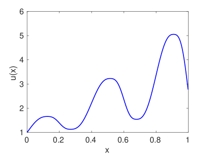
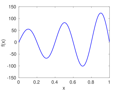
Figure 2: Solution field $u(x)$ of Forchheimer equation (left panel) and force term $f(x)$ (right panel).

We then study the convergence behavior of our different methods. Figure 3 shows how the relative error decays for the different methods and for a decomposition into 20 subdomains (left panel) and 50 subdomains (right panel). The initial guess is equal to zero for all these methods.

Figure 3: Convergence behavior for Newton’s method, NKRAS, nonlinear RAS, nonlinear SRAS, RASPEN and SRASPEN applied to Forchheimer equation. On the left, the simulation refers to a decomposition into 20 subdomains while on the right we consider 50 subdomains. The mesh size is $h=10^{-3}$ and the overlap is $8h$.

Both plots in Figure 3 show that the convergence rate of iterative nonlinear RAS and nonlinear SRAS is the same and very slow. As expected, NKRAS with line search converges better than Newton’s method. Further, RASPEN and SRASPEN converge in the same number of outer Newton iterations. Moreover, it seems that the convergence of RASPEN and SRASPEN is not affected by the number of subdomains. However, these plots do not tell the whole story, as one should focus not only on the number of iterations but also on the cost of each iteration. To compare the cost of an iteration of RASPEN and SRASPEN, we have to distinguish two cases, that is, if one solves the Jacobian system directly or with some Krylov methods, e.g., GMRES. First, suppose that we want to solve the Jacobian system with a direct method and thus we need to assemble and store the Jacobians. From the expressions in equation (32) we remark that the assembly of the Jacobian of RASPEN requires $N\times N_{v}$ subdomain solves, where $N$ is the number of subdomains and $N_{v}$ is the number of unknowns in volume. On the other hand, the assembly of the Jacobian of SRASPEN requires $N\times\overline{N}$ solves, where $\overline{N}$ is the number of unknowns on the substructures and $\overline{N}\ll N_{v}$. Thus, while the assembly of $J_{\mathcal{F}}$ is prohibitive, it can still be affordable to assemble $J_{\overline{\mathcal{F}}}$. Further, the direct solution of the Jacobian system is feasible as $J_{\overline{\mathcal{F}}}$ has size $\overline{N}\times\overline{N}$. Suppose now that we solve the Jacobian systems with GMRES. Let us indicate with $I(k)$ and $I^{S}(k)$ the number of GMRES iterations to solve the volume and substructured Jacobian systems at the $k$-th outer Newton iteration. Each GMRES iteration requires $N$ subdomain solves which can be performed in parallel. In our numerical experiment, we have observed that generally $I^{S}(k)\leq I(k)$, with $I(k)-I^{S}(k)\approx 0,1,2$, that is GMRES requires the same number of iterations or slightly less to solve the substructured Jacobian system compared to the volume one.

To better compare these two methods, we follow [15] and introduce the quantity $L(n)$ which counts the number of subdomain solves performed by these two methods till iteration $n$, taking into account the advantages of a parallel implementation. We set $L(n)=\sum_{k=1}^{n}L_{in}^{k}+I(k)$, where $L_{in}^{k}$ is the maximum over the subdomains of the number of Newton iterations required to solve the local subdomain problems at iteration $k$. The number of linear solves performed by GMRES should be $I(k)\times N$, but as the $N$ linear solves can be performed in parallel, the total cost of GMRES corresponds approximately to $I(k)$ linear solves. Figure 4 shows the error decay as a function of $L(n)$. We note that the two methods require approximately the same computational cost and SRASPEN is slightly faster.

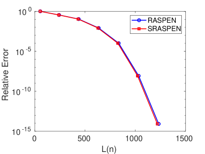
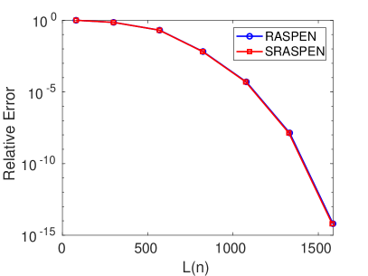
Figure 4: Relative error decay for RASPEN and SRASPEN applied to Forchheimer equation with respect to the number of linear solves. On the left, the simulation refers to a decomposition into 20 subdomains while on the right we consider 50 subdomains. The mesh size is $h=10^{-3}$.

For the decomposition into 50 subdomains, RASPEN requires on average 91.5 GMRES iterations per Newton iteration, while SRASPEN requires an average of 90.87 iterations. The size of the substructured space $\overline{V}$ is $\overline{N}=98$. For the decomposition into 20 subdomains, RASPEN requires an average of 40 GMRES iterations per Newton’s iteration, while SRASPEN needs 38 iterations. The size of $\overline{V}$ is $\overline{N}=38$, which means that GMRES reaches the given tolerance of $10^{-12}$ after exactly $\overline{N}$ steps, which is the size of the substructured Jacobian. Under these circumstances, it can be convenient to actually assemble $J_{\overline{\mathcal{F}}}$, as it requires $\overline{N}\times N$ subdomain solves which is the total cost of GMRES. Furthermore, the $\overline{N}\times N$ subdomain solves are embarrassingly parallel, while the $\overline{N}\times N$ solves of GMRES can be parallelized in the spatial direction, but not in the iterative one. As future work, we believe it will be interesting to study the convergence of a Quasi-Newton method based on SRASPEN, where one assembles the Jacobian substructured matrix after every few outer Newton iterations, reducing the overall computational cost.

As a final remark, we specify that Figure 4 has been obtained setting a zero initial guess for the nonlinear subdomain problems. However, at the iteration $k$ of RASPEN one can use the subdomain restriction of the updated volume solution, that is $R_{j}\mathbf{u}^{k-1}$, which has been obtained by solving the volume Jacobian system at iteration $k-1$, and is thus generally a better initial guess for the next iteration. On the other hand in SRASPEN, one could use the subdomain solutions computed at iteration $k-1$, i.e. $\mathbf{u}_{i}^{k-1}$, as initial guess for the nonlinear subdomain problems, as the substructured Jacobian system corrects only the substructured values. Numerical experiments showed that with this particular choice of initial guess for the nonlinear subdomain problems, SRASPEN requires generally more Newton iterations to solve the local problems. In this setting, there is not a method that is constantly faster than the other as it depends on a delicate trade-off between the better GMRES performance and the need to perform more Newton iterations for the nonlinear local problems in SRASPEN.

6.3 Nonlinear Diffusion

In this subsection we consider the nonlinear diffusion problem on a square domain $\Omega:=(0,1)^{2},$

(42) $$-\nabla\cdot\left(1+u(x)^{2}\right)\nabla u(x) =f,\quad\text{ in }\Omega,$$

$$u(x) =g(x)\quad\text{on }\partial\Omega,$$

where the right hand side $f$ is chosen such that $u(x)=\sin(\pi x)\sin(\pi y)$ is the exact solution. We start all these methods with an initial guess $u^{0}(x)=10^{5}$, so that we start far away from the exact solution, and hence Newton’s method exhibits a long plateau before quadratic convergence begins.

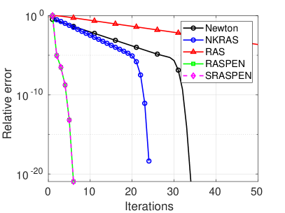
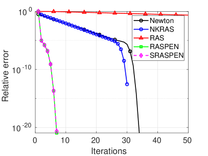
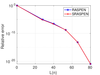
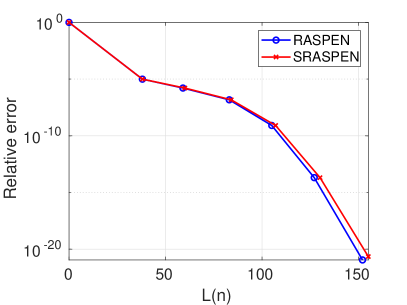
Figure 5: Relative error decay versus the number of iterations (top row) and error decay versus the number of linear solves (bottom row). The left figures refer to a decomposition into four subdomains, the right figures to a decomposition into 25 subdomains. The mesh size is $h=0.012$ and the overlap is $8h$.

Figure 5 shows the convergence behavior for the different methods as function of the number of iterations and the number of linear solves. The average number of GMRES iterations is 8.1667 for both RASPEN and SRASPEN for the four subdomain decomposition. For a decomposition into 25 subdomains, the average number of GMRES iterations is 19.14 for RASPEN and 19.57 for SRASPEN. We remark that as the number of subdomains increases, GMRES needs more iterations to solve the Jacobian system. This is consistent with the interpretation of (32) as a Jacobian matrix $J\left(\mathbf{u}^{(j)}\right)$ preconditioned by the additive operator $\sum_{j\in\mathcal{J}}\left(R_{j}J\left(\mathbf{u}^{(j)}\right)P_{j}\right)^{-1}$; We expect this preconditioner not to be scalable since it does not involve a coarse correction.

We conclude this section by showing the convergence behavior for the two-level variants of nonlinear RAS, nonlinear SRAS, RASPEN, and SRASPEN. We use a coarse grid in volume taking half of the points in $x$ and $y$, and a coarse substructured grid taking half of the unknowns as depicted in Figure 1. The interpolation and restriction operators $P_{0},R_{0},\overline{P}_{0}$ and $\overline{R}_{0}$ are the classical linear interpolation and fully weighting restriction operators defined in Section 5. From Figure 6,

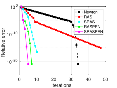
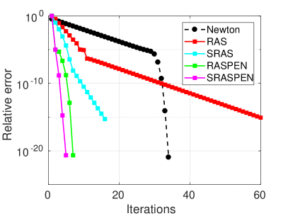
Figure 6: Relative error decay versus the number of iterations for Newton’s method, iterative two-level nonlinear RAS and SRAS, and the two-level variants of RASPEN and SRASPEN. The left figure refers to a decomposition into 4 subdomains, while the right figure refers to a decomposition into 16 subdomains. The mesh size is $h=0.012$ and the overlap is $4h$.

we note that two-level nonlinear SRAS is much faster than two-level nonlinear RAS, and this observation is in agreement with the linear case treated in [12, 11]. Since the two-level iterative methods are not equivalent, we also remark that two-level SRASPEN shows a better performance than two-level RASPEN in terms of iteration count. As the one-level smoother is the same in all methods, the better convergence of the substructured methods implies that the coarse equation involving $\overline{\mathcal{F}}_{0}$ provides a much better coarse correction than the classical volume one involving $F_{0}$.

Even though the two-level substructured methods are faster in terms of iteration count, the solution of the FAS problem involving $\overline{\mathcal{F}}_{0}=\overline{R}_{0}\overline{\mathcal{F}}(\overline{P}_{0}(\mathbf{v}_{0}))$ is rather expensive as it requires to evaluate twice the substructured function $\overline{\mathcal{F}}$ (each evaluation requires subdomain solves) to compute the right hand side, to solve a Jacobian system involving $J_{\overline{\mathcal{F}}_{0}}$, and to evaluate $\overline{\mathcal{F}}$ on the iterates, which again require the solution of subdomain problems. Unless one has a fully parallel implementation available, the coarse correction involving $\overline{\mathcal{F}}_{0}$ is doomed to represent a bottleneck.

7 Conclusions

We presented for the first time an analysis of the effects of substructuring on RAS when it is applied as an iterative solver and as a preconditioner. We proved that iterative RAS and iterative SRAS converge at the same rate, both in the linear and nonlinear case. For the nonlinear case, we showed that the preconditioned methods, namely RASPEN and SRASPEN also have the same rate of convergence as they produce the same iterates once these are restricted to the interfaces. Surprisingly, the equivalence between volume and substructured RAS breaks down when they are considered as preconditioners for Krylov methods. We showed that the Krylov spaces are equivalent, once the volume one is restricted to the substructure, however we obtained that the iterates are different by carefully deriving the least squares problems solved by GMRES. Our analysis shows that GMRES should always be applied to the substructured system as it converges similarly when applied to the volume formulation, but needs much less memory. This allows us to state that, while nonlinear RASPEN and SRASPEN produce the same iterates, SRASPEN has advantages when solving the Jacobian system, either because the use of a direct solve is feasible, or because the Krylov method can work at the substructured level. Finally, we introduced substructured two-level nonlinear SRAS and SRASPEN, and showed numerically that these methods have better convergence properties than their volume counterparts in terms of iteration count, although they are quite expensive in the present form per iteration. Future efforts will be in the direction of approximating $\overline{\mathcal{F}}_{0}$, by replacing the function $\overline{\mathcal{F}}$, which is defined on a fine mesh, with an approximation on a very coarse mesh, thus reducing the overall cost of the substructured coarse correction, or by using spectral coarse spaces.

References

- [1] A. Brandt and O. E. Livne, Multigrid Techniques, Society for Industrial and Applied Mathematics, 2011.
- [2] X.-C. Cai and M. Dryja, Domain decomposition methods for monotone nonlinear elliptic problems, Contemporary Mathematics, 180 (1994).
- [3] X.-C. Cai and D. E. Keyes, Nonlinearly preconditioned inexact Newton algorithms, SIAM Journal on Scientific Computing, 24 (2002), pp. 183–200.
- [4] X.-C. Cai, D. E. Keyes, and D. P. Young, A nonlinear additive Schwarz preconditioned inexact Newton method for shocked duct flow, in Proceedings of the 13th International Conference on Domain Decomposition Methods, Citeseer, 2001.
- [5] X.-C. Cai and X. Li, Inexact Newton methods with restricted additive Schwarz based nonlinear elimination for problems with high local nonlinearity, SIAM Journal on Scientific Computing, 33 (2011), pp. 746–762.
- [6] X.-C. Cai and M. Sarkis, A restricted additive Schwarz preconditioner for general sparse linear systems, SIAM Journal on Scientific Computing, 21 (1999), pp. 792–797.
- [7] F. Chaouqui, M. J. Gander, P. M. Kumbhar, and T. Vanzan, On the nonlinear Dirichlet-Neumann method and preconditioner for Newton’s method, arXiv:2103.12203, (2021), https://arxiv.org/abs/2103.12203.
- [8] G. Ciaramella and M. J. Gander, Iterative Methods and Preconditioners for Systems of Linear Equations, SIAM, 2021.
- [9] G. Ciaramella, M. Hassan, and B. Stamm, On the scalability of the Schwarz method, The SMAI journal of computational mathematics, 6 (2020), pp. 33–68, https://doi.org/10.5802/smai-jcm.61.
- [10] G. Ciaramella and T. Vanzan, Substructured two-level and multi-level domain decomposition methods, arXiv:1908.05537v2, (2019), https://arxiv.org/abs/1908.05537.
- [11] G. Ciaramella and T. Vanzan, Spectral substructured two-level domain decomposition methods, (submitted, 2020).
- [12] G. Ciaramella and T. Vanzan, Substructured two-grid and multi-grid domain decomposition methods, (submitted 2020).
- [13] B. Cockburn and J. Gopalakrishnan, A characterization of hybridized mixed methods for second order elliptic problems, SIAM Journal on Numerical Analysis, 42 (2004), pp. 283–301.
- [14] P. Deuflhard, Newton Methods for Nonlinear Problems: Affine Invariance and Adaptive Algorithms, Springer Series in Computational Mathematics, Springer Berlin Heidelberg, 2010.
- [15] V. Dolean, M. J. Gander, W. Kheriji, F. Kwok, and R. Masson, Nonlinear preconditioning: How to use a nonlinear Schwarz method to precondition Newton’s method, SIAM Journal on Scientific Computing, 38 (2016), pp. A3357–A3380.
- [16] C. Farhat and F.-X. Roux, A method of finite element tearing and interconnecting and its parallel solution algorithm, International journal for numerical methods in engineering, 32 (1991), pp. 1205–1227.
- [17] M. J. Gander, Optimized Schwarz methods, SIAM Journal on Numerical Analysis, 44 (2006), pp. 699–731.
- [18] M. J. Gander, Schwarz methods over the course of time, Electronic transactions on numerical analysis, 31 (2008), pp. 228–255.
- [19] M. J. Gander, On the origins of linear and non-linear preconditioning, in Domain Decomposition Methods in Science and Engineering XXIII, C.-O. Lee, X.-C. Cai, D. E. Keyes, H. H. Kim, A. Klawonn, E.-J. Park, and O. B. Widlund, eds., Cham, 2017, Springer International Publishing, pp. 153–161.
- [20] M. J. Gander and L. Halpern, Méthodes de décomposition de domaines – notions de base, Editions TI, Techniques de l’Ingénieur, France, (2012).
- [21] S. Gong and X.-C. Cai, A nonlinear elimination preconditioned Newton method with applications in arterial wall simulation, in International Conference on Domain Decomposition Methods, Springer, 2017, pp. 353–361.
- [22] S. Gong and X.-C. Cai, A nonlinear elimination preconditioned inexact Newton method for heterogeneous hyperelasticity, SIAM Journal on Scientific Computing, 41 (2019), pp. S390–S408.
- [23] W. Hackbusch, Multi-Grid Methods and Applications, Springer Series in Computational Mathematics, Springer Berlin Heidelberg, 2013.
- [24] A. Klawonn, M. Lanser, B. Niehoff, P. Radtke, and O. Rheinbach, Newton-Krylov-FETI-DP with adaptive coarse spaces, in Domain Decomposition Methods in Science and Engineering XXIII, C.-O. Lee, X.-C. Cai, D. E. Keyes, H. H. Kim, A. Klawonn, E.-J. Park, and O. B. Widlund, eds., Cham, 2017, Springer International Publishing, pp. 197–205.
- [25] A. Klawonn, M. Lanser, and O. Rheinbach, Nonlinear FETI-DP and BDDC methods, SIAM Journal on Scientific Computing, 36 (2014), pp. A737–A765.
- [26] A. Klawonn and O. Widlund, FETI and Neumann-Neumann iterative substructuring methods: connections and new results, Communications on Pure and Applied Mathematics: A Journal Issued by the Courant Institute of Mathematical Sciences, 54 (2001), pp. 57–90.
- [27] P. J. Lanzkron, D. J. Rose, and J. T. Wilkes, An analysis of approximate nonlinear elimination, SIAM Journal on Scientific Computing, 17 (1996), pp. 538–559.
- [28] S.-H. Lui, On Schwarz alternating methods for nonlinear elliptic PDEs, SIAM Journal on Scientific Computing, 21 (1999), pp. 1506–1523.
- [29] S.-H. Lui, On monotone iteration and Schwarz methods for nonlinear parabolic PDEs, Journal of computational and applied mathematics, 161 (2003), pp. 449–468.
- [30] L. Luo, X.-C. Cai, Z. Yan, L. Xu, and D. E. Keyes, A multilayer nonlinear elimination preconditioned inexact newton method for steady-state incompressible flow problems in three dimensions, SIAM Journal on Scientific Computing, 42 (2020), pp. B1404–B1428.
- [31] J. Mandel and M. Brezina, Balancing domain decomposition for problems with large jumps in coefficients, Mathematics of Computation, 65 (1996), pp. 1387–1401.
- [32] J. S. Przemieniecki, Matrix structural analysis of substructures, AIAA Journal, 1 (1963), pp. 138–147.
- [33] A. Quarteroni and A. Valli, Domain Decomposition Methods for Partial Differential Equations, Numerical Mathematics and Scientific Computation, Oxford Science Publications, 1999.
- [34] Y. Saad, Iterative methods for sparse linear systems, SIAM, 2003.
- [35] A. Toselli and O. Widlund, Domain Decomposition Methods: Algorithms and Theory, vol. 34 of Series in Computational Mathematics, Springer, New York, 2005.
- [36] U. Trottenberg, C. Oosterlee, and A. Schuller, Multigrid, Elsevier Science, 2000.