Convergence Properties of the Distributed Projected Subgradient Algorithm over General Graphs

Abstract

In this paper, we revisit a well-known distributed projected subgradient algorithm which aims to minimize a sum of cost functions with a common set constraint. In contrast to most of existing results, weight matrices of the time-varying multi-agent network are assumed to be more general, i.e., they are only required to be row stochastic instead of doubly stochastic. We focus on analyzing convergence properties of this algorithm under general graphs. We first show that there generally exists a graph sequence such that the algorithm is not convergent when the network switches freely within finitely many general graphs. Then to guarantee the convergence of this algorithm under any uniformly jointly strongly connected general graph sequence, we provide a necessary and sufficient condition, i.e., the intersection of optimal solution sets to all local optimization problems is not empty. Furthermore, we surprisingly find that the algorithm is convergent for any periodically switching general graph sequence, and the converged solution minimizes a weighted sum of local cost functions, where the weights depend on the Perron vectors of some product matrices of the underlying periodically switching graphs. Finally, we consider a slightly broader class of quasi-periodically switching graph sequences, and show that the algorithm is convergent for any quasi-periodic graph sequence if and only if the network switches between only two graphs.

I Introduction

In the past decade, distributed convex optimization has received intensive research attention, motivated by its broad applications in various areas including distributed estimation [1], resource allocation [2], and machine learning [3]. The basic idea is that in a multi-agent network, all agents cooperate to solve an optimization problem with their local cost functions, constraints and neighbors’ states. A variety of distributed algorithms have been designed for different formulations. By performing local averaging operations and taking subgradient descent steps, a distributed subgradient algorithm was proposed for unconstrained distributed optimization problems in [4]. Then a projected subgradient algorithm was developed to deal with a common set constraint in [5]. The case of nonidentical set constraints was studied in [6, 7]. Following that, by combining projected subgradient methods and primal-dual ideas, distributed primal-dual subgradient algorithms were designed to minimize a sum of local cost functions with set constraints, local inequality and equality constraints [8]. Moreover, distributed primal-dual algorithms have also been explored for coupled constraints [9, 10].

For a distributed algorithm, the communication topology of the multi-agent network has a great effect on its convergence [11]. Since the pioneering work for distributed optimization in [4], weight-balanced graphs have been widely employed to design distributed algorithms [12, 13, 10, 8]. In [10], undirected and connected graphs were adopted for distributed primal-dual algorithms. Based on saddle-point dynamics, a continuous-time algorithm was proposed under strongly connected and weight-balanced digraphs in [12]. Time-varying weight-balanced graphs have also been utilized for the distributed design [13, 8].

Plenty of results on distributed optimization were obtained under weight-balanced graphs because there usually existed a common Lyapunov function to facilitate the convergence analysis [14, 4, 15]. Furthermore, most of (sub)gradient-based algorithms could achieve an optimal solution under weight-balanced graphs because Perron vectors of weight matrices were with identical entries [6, 7, 4]. However, a weight-balanced graph requires the in-degree of each node being equal to its out-degree, and is not always practical in real applications [11]. For instance, if agents use broadcast-based communications in a wireless network, they neither know their out-neighbors nor are able to adjust their outgoing weights. Thus, the weight-balance condition is difficult to be guaranteed in this case [7]. To overcome the difficulty, some new mechanisms have been explored to design distributed algorithms under weigh-unbalanced graphs [7, 16, 17, 18]. In [18], a reweighting technique was proposed for fixed graphs with known Perron vectors. By combining the dual averaging algorithm with the push-sum consensus protocol, a distributed push-sum method was developed in [17]. Requiring a row stochastic and a column stochastic matrices, a distributed push-pull algorithm was designed in [16], where for individual agent, the gradient was pushed to its neighbors, and the decision variable was pulled from its neighbors. In [19, 7], heterogeneous stepsizes were adopted to balance the graph.

Some researches have been focused on developing distributed algorithms under weight-unbalanced graphs. However, how do unbalanced networks affect the performance of a distributed algorithm? Note that it is an important problem because it can provide us with a better understanding of existing works, and moreover, guide us to design effective distributed algorithms.

In this paper, we revisit a well-known distributed projected subgradient algorithm, proposed in [5], to minimize a sum of (nonsmooth) cost functions with a common set constraint. Compared with existing results in [20, 5], we assume the time-varying communication network being general (weight matrices of the network are row stochastic instead of doubly stochastic), and focus on analyzing convergence properties of this algorithm. Our main contributions are summarized as follows.

• We show that there generally exists a graph sequence such that the algorithm is not convergent if the time-varying network switches freely within finitely many general graphs.

• To guarantee the convergence of this algorithm for any uniformly jointly strongly connected general graph sequence, we provide a necessary and sufficient condition, namely, the intersection of optimal solution sets to all local optimization problems is not empty.

• We find that the algorithm is convergent for any periodically switching general graph sequence, and moreover, the converged solution minimizes a weighted sum of the local cost functions. In addition, we relax the periodic condition slightly, and define a broader class of quasi-periodic graph sequences. We show that the algorithm is always convergent for any quasi-periodic graph sequence if and only if the network switches between two graphs.

The remainder of this paper is organized as follows. Some preliminary knowledge related to convex analysis and graph theory is introduced in Section 2, and then the problem is formulated in Section 3. Our main results are presented Sections 4, while their rigorous proofs are provided in Section 5. Following that, illustrative examples are carried out in Section 6. Finally, concluding remarks are given in Section 7.

Notations: Let $\mathbb{R}$, $\mathbb{R}^{m}$ and $\mathbb{R}^{m\times n}$ be the set of real numbers, the set of $m$-dimensional real column vectors, and the set of $m$-by-$n$ dimensional real matrices, respectively. Let $\mathbb{N}$ be the set of nonnegative integers. Vectors are column vectors by default. $x^{\prime}$ stands for the transpose of vector $x$. $[A]_{ij}$ means the $(i,j)$-th entry of matrix $A$. The Euclidean norm of $x,y\in\mathbb{R}^{m}$ is defined by $x^{\prime}y$. Let $|\cdot|$, $|\cdot|_{1}$ be the Euclidean norm and $l_{1}$-norm of a vector, respectively. Denote ${\rm dist}(x,\Omega)$ as the distance from a point $x$ to a set $\Omega$ (that is, ${\rm dist}(x,\Omega)\triangleq\inf_{y\in\Omega}|y-x|$).

II Preliminary knowledge

In this section, we introduce some basic concepts related to convex analysis and graph theory.

II-A Convex analysis

A set $\Omega\subset\mathbb{R}^{m}$ is convex if $\lambda x+(1-\lambda)y\in\Omega$ for all $x,y\in\Omega$ and $\lambda\in[0,1]$. For a closed convex set $\Omega\subset\mathbb{R}^{m}$, we define $P_{\Omega}(\cdot):\mathbb{R}^{m}\rightarrow\Omega$ as a projection operator which maps $x\in\mathbb{R}^{m}$ to a unique point $P_{\Omega}(x)$ such that $P_{\Omega}(x)={\rm argmin}_{y\in\Omega}|x-y|$. Referring to Lemma 1 in [5], we have

$$|P_{\Omega}(x)-y|\leq|x-y|,~{}\forall x\in\mathbb{R}^{m},~{}\forall y\in\Omega,$$ (1)

and moreover,

$$|P_{\Omega}(x)-y|^{2}\leq|x-y|^{2}-|x-P_{\Omega}(x)|^{2},~{}\forall x\in\mathbb{R}^{m},~{}\forall y\in\Omega.$$ (2)

A function $f:\Omega\rightarrow\mathbb{R}$ is convex if $\Omega$ is a convex set, and

$$f(\theta x+(1-\theta)y)\leq\theta f(x)+(1-\theta)f(y),~{}\forall x,y\in\Omega,~{}\forall\theta\in[0,1].$$

Furthermore, it is strictly convex if the strict inequality holds whenever $x\not=y$ and $\theta\in(0,1)$. If $g_{f}(x)\in\mathbb{R}^{m}$ satisfies

$$f(y)-f(x)\geq(y-x)^{\prime}g_{f}(x),$$

then $g_{f}(x)$ is the subgradient of $f$ at $x$. Denoted by $\partial f(x)$ the set of all subgradients of $f$ at $x$.

II-B Graph theory

The communication topology of a multi-agent network can be modeled by a digraph $\mathcal{G}(\mathcal{V},\mathcal{E})$, where $\mathcal{V}$ is the node set, and $\mathcal{E}$ is the edge set. Then a nonnegative weight matrix $A=[a_{ij}]$ can be associated with $\mathcal{G}$, where $a_{ij}>0$ if and only if $(j,i)\in\mathcal{E}$. Conversely, a graph $\mathcal{G}$ can also be associated with a nonnegative matrix $A$. Node $j$ is a neighbor of $i$, and can send information to $i$ if $a_{ij}>0$. Suppose that there are self-loops in $\mathcal{G}$, i.e., $a_{ii}>0$ for all $i\in\mathcal{V}$. Graph $\mathcal{G}$ is said to be weight-balanced if $\sum_{j\in\mathcal{V}}a_{ij}=\sum_{j\in\mathcal{V}}a_{ji}$ for $i\in\mathcal{V}$, and is weight-unbalanced otherwise. A path from $i_{1}$ to $i_{p}$ is defined by an edge sequence $(i_{1},i_{2}),(i_{2},i_{3}),\dots,(i_{p-1},i_{p})\in\mathcal{E}$ with distinct nodes $i_{1},\dots,i_{p}$. $\mathcal{G}$ is strongly connected if there exists at least a path between every pair of nodes. If a network is time-varying, we denote $\mathcal{G}(\mathcal{V},\mathcal{E}(k))$ or $\mathcal{G}(k)$ as the graph at time slot $k$. Furthermore, the joint graph over the time interval $[k_{1},k_{2})$ is given by $\mathcal{G}([k_{1},k_{2}))\triangleq\mathcal{G}(\mathcal{V},\bigcup_{k\in[k_{1},k_{2})}\mathcal{E}(k))$.

A vector is said to be stochastic if it is with nonnegative entries and the sum of its entries is $1$. Furthermore, it is also positive if all entries of the vector are positive. A matrix is row (column) stochastic if all of its row (column) vectors are stochastic, and is doubly stochastic if it is both row and column stochastic. A row stochastic matrix is also sometimes simply called a stochastic matrix. The following result, collected from Lemma $5.3$ in [19], addresses the relationship of positive stochastic vectors and stochastic matrices.

Lemma 1.

For any positive stochastic vector $\mu\in\mathbb{R}^{n}$, there must be a stochastic matrix $A=(a_{ij})\in\mathbb{R}^{n\times n}$ such that $\mu^{\prime}A=\mu^{\prime}$, and moreover, the graph associated with $A$ is strongly connected.

Let $B\in\mathbb{R}^{n\times n}$ be a stochastic matrix, and $\mathcal{G}_{B}$ be the associated graph. It follows from the Perron-Frobenius theorem [21] that there is a unique positive stochastic left eigenvector $\mu(B)$ of $B$ associated with eigenvalue $1$ if $\mathcal{G}_{B}$ is strongly connected. We call $\mu(B)$ the Perron vector of $B$.

III Formulation and algorithm

In this section, we formulate the constrained distributed optimization problem, and then revisit a projected subgradient algorithm. Furthermore, we give the problem statement.

Consider a network of $n$ agents connected by a time-varying digraph $\mathcal{G}(\mathcal{V},\mathcal{E}(k))$ (or simply $\mathcal{G}(k)$), where $\mathcal{V}=\{1,\dots,n\}$ and $\mathcal{E}(k)\subset\mathcal{V}\times\mathcal{V}$. For each $i\in\mathcal{V}$, there is a local (nonsmooth) cost function $f_{i}:\mathbb{R}^{m}\rightarrow\mathbb{R}$ and a feasible constraint set $X\subset\mathbb{R}^{m}$. All agents cooperate to minimize the global cost function $\sum_{i\in\mathcal{V}}f_{i}(x)$ in $X$. To be strict, the problem can be formulated as

$${\rm min}~{}~{}\sum_{i\in\mathcal{V}}f_{i}(x),\quad{\rm s.t.}~{}~{}x\in X,$$ (3)

where $x$ is the decision variable.

Let $x_{i}(k)$ be the estimation for a solution to (3) by agent $i$. Then a distributed algorithm is said to achieve a solution to (3) if for any initial condition $x_{i}(0)\in\mathbb{R}^{m}$, $\lim_{k\to\infty}|x_{i}(k)-x_{j}(k)|=0$, and moreover, there exists $x^{*}\in X^{*}$ such that $\lim_{k\to\infty}|x_{i}(k)-x^{*}|=0$, where

$$X^{*}=\Big{\{}z~{}|~{}z={\rm argmin}_{x\in X}\sum_{i\in\mathcal{V}}f_{i}(x)\Big{\}}.$$

To ensure the well-posedness of (3), we make the following standard assumptions.

Assumption 1.

(Convexity) For each $i\in\mathcal{V}$, $f_{i}$ is a convex function on an open set containing $X$, and $X$ is a closed convex set.

Assumption 2.

(Boundedness of Subgradients) For each $i\in\mathcal{V}$, the subgradient set of $f_{i}$ is bounded over $X$, i.e., there exists a scalar $L>0$ such that

$$|d|\leq L,~{}\forall d\in\partial f_{i}(x),~{}\forall x\in X.$$ (4)

Assumption 3.

(Connectivity) The graph sequence $\mathcal{G}(k)$ is uniformly jointly strongly connected (UJSC), i.e., there exist an integer $B>0$ such that the joint graph $\mathcal{G}([k,k+B))$ is strongly connected for $k\in\mathbb{N}$.

Assumption 4.

(Weight Rule)

1. The weight matrix $A(k)=[a_{ij}(k)]$ associated to $\mathcal{G}(k)$ is stochastic, i.e.,
   $\sum_{j\in\mathcal{V}}a_{ij}(k)=1$ for $i\in\mathcal{V}$ and $k\in\mathbb{N}$.

2. There is a scalar $0<\eta<1$ such that $a_{ij}(k)\geq\eta$ if $a_{ij}(k)>0$, and $a_{ii}(k)\geq\eta$ for $i,j\in\mathcal{V}$ and $k\in\mathbb{N}$.

Note that (3) is a well-known constrained distributed optimization problem investigated in [22, 5, 23]. A pioneering distributed algorithm for this problem is the projected subgradient method, which combines an average step with a local projected gradient update step [5]. The specific form of this algorithm is given by

$$v_{i}(k)= \sum_{j\in\mathcal{V}}a_{ij}(k)x_{j}(k),$$ (5)

$$x_{i}(k+1)= P_{X}(v_{i}(k)-\alpha_{k}d_{i}(k)),$$

where $d_{i}(k)\in\partial f_{i}(v_{i}(k))$, and $\alpha_{k}>0$ is the stepsize. To guarantee the convergence of (5), the following assumption is made [5].

Assumption 5.

(Stepsize Rule) $\sum_{k=0}^{\infty}\alpha_{k}=\infty$, and moreover, $\sum_{k=0}^{\infty}\alpha^{2}_{k}<\infty$.

Remark 1.

In fact, Assumptions 1-5 have also been employed in [20, 19, 5, 8]. As a comparison, we only suppose that the weight matrix $A(k)$ is row stochastic instead of doubly stochastic, i.e., the communication graph may be weight-unbalanced. Thus, the considered problem is more general.

The following result, proved in [5], shows a convergence property of (5).

Proposition 1.

Let Assumptions 1-5 hold. If $A(k)$ is also column stochastic for $k\in\mathbb{N}$, then algorithm (5) achieves a solution to (3).

Proposition 1 indicates the convergence of (5) under graphs with doubly stochastic weight matrices. Following that, great efforts have been paid to develop distributed algorithms over weight-balanced graphs [12, 24, 8]. Furthermore, some new mechanisms have been proposed to replace the weight-balance assumption including the push-sum protocol [17] and the push-pull method [16]. To distinguish with weight-balanced graphs, we call a graph being general if its weight matrix is only required to be row stochastic. An interesting question is what the convergence performance of a distributed algorithm is if the underlying graph is general. In this paper, taking (5) as a starting point, we explore its convergence under general graphs. To be specific, we are interested in the following three questions.

• Is algorithm (5) convergent under general graphs?

• If it is, which solution does it converge to? If not, under what condition on the cost functions it is convergent?

• Is there any class of general graph sequences under which the algorithm (5) is convergent?

IV Main results

In this section, we present the main results on the convergence of (5) under general graph sequences. At the beginning, we show that there generally exists a graph sequence such that (5) is not convergent. Then we provide a necessary and sufficient condition to guarantee its convergence. Finally, we establish its convergence under periodic and quasi-periodic graph sequences.

IV-A Basic results

Define $y(k)=\frac{1}{n}\sum_{i\in\mathcal{V}}x_{i}(k)$ as the average of agents’ estimations. The following lemma, proved in Section V-B, shows consensus results of (5).

Lemma 2.

Consider algorithm (5). Under Assumptions 2-4, the following statements hold.

1. If the stepsize satisfies $\lim_{k\to\infty}\alpha_{k}=0$, then

   $$\lim_{k\to\infty}|x_{i}(k)-y(k)|=0,~{}\forall i\in\mathcal{V}.$$

2. If the stepsize satisfies $\sum_{k=0}^{\infty}\alpha_{k}^{2}<\infty$, then

   $$\sum_{k=0}^{\infty}\alpha_{k}|x_{i}(k)-y(k)|<\infty,~{}\forall i\in\mathcal{V}.$$

Clearly, (5) can be rewritten as

$$x_{i}(k+1)=\sum_{j\in\mathcal{V}}a_{ij}(k)x_{j}(k)+\omega_{i}(k),$$ (6)

where $\omega_{i}(k)=P_{X}(v_{i}(k)-\alpha_{k}d_{i}(k))-v_{i}(k)$. In fact, (6) is a consensus dynamics with disturbance $\omega_{i}(k)$. Combining (17) with $\lim_{k\to\infty}\alpha_{k}=0$, we obtain $\lim_{t\to\infty}\omega_{i}(k)=0$. For such a dynamics, consensus can be achieved under a UJSC graph sequence as discussed in [25, 26]. However, Lemma 2 (ii), indicating the consensus rate, has not been proved in [25, 26].

Referring to Theorem 1 in [6], we have the following result for (5) under a fixed digraph.

Lemma 3.

Consider the graph sequence given by $\mathcal{G}(k)=\mathcal{G}_{A}$ for $k\in\mathbb{N}$, where $\mathcal{G}_{A}$ is a strongly connected graph associated with weight matrix $A=[a_{ij}]$. Suppose that $\sum_{j\in\mathcal{V}}a_{ij}=1$ for all $i\in\mathcal{V}$. Under Assumptions 1, 2 and 5, algorithm (5) achieves a solution to

$$\min~{}~{}\sum_{i\in\mathcal{V}}\mu_{i}(A)f_{i}(x),\quad{\rm s.t.}~{}~{}x\in X,$$ (7)

where $\mu(A)=[\mu_{1}(A),\dots,\mu_{n}(A)]^{\prime}$ is the Perron vector of $A$ such that $\mu(A)^{\prime}A=\mu(A)^{\prime}$.

Remark 2.

Lemma 3 implies that (5) optimizes a weighted sum of the local cost functions if $\mathcal{G}(k)$ is fixed. In fact, the result can be directly extended as follows. Let $\mathcal{G}_{A_{1}},\dots,\mathcal{G}_{A_{p}}$ be strongly connected graphs with an identical Perron vector $\mu(A)$. Consider a time-varying graph sequence $\mathcal{G}(k)$, which switches within $\{\mathcal{G}_{A_{1}},\dots,\mathcal{G}_{A_{p}}\}$, i.e., $\mathcal{G}(k)\in\{\mathcal{G}_{A_{1}},\dots,\mathcal{G}_{A_{p}}\}$ for all $k\in\mathbb{N}$. If Assumptions 1, 2, 4 and 5 hold, then algorithm (5) achieves a solution to (7). The proof is similar to that of Theorem 1 in [6], and is omitted here.

IV-B Convergence analysis

In this section, we analyze whether (5) is still convergent in the absence of doubly stochastic weight matrices for the communication network.

Let $\mathcal{G}_{A_{1}},\dots,\mathcal{G}_{A_{p}}$ be strongly connected graphs with weight matrices $A_{1},\dots,A_{p}$, respectively. We define $\mu(A_{l})=[\mu_{1}(A_{l}),\dots,\mu_{n}(A_{l})]^{\prime}$ as the Perron vectors of $A_{l}$ for $l\in\{1,\dots,p\}$, and moreover,

$$X_{\mu(A_{l})}^{*}\triangleq\Big{\{}z~{}|~{}z={\rm argmin}_{x\in X}\sum_{i\in\mathcal{V}}\mu_{i}(A_{l})f_{i}(x)\Big{\}}.$$ (8)

Then we have the following result, whose proof can be found in Section V-C.

Theorem 1.

Let Assumptions 1, 2, 4 and 5 hold. Consider a time-varying graph $\mathcal{G}(k)$, which switches within $\{\mathcal{G}_{A_{1}},\dots,\mathcal{G}_{A_{p}}\}$, i.e., $\mathcal{G}(k)\in\{\mathcal{G}_{A_{1}},\dots,\mathcal{G}_{A_{p}}\}$ for all $k\in\mathbb{N}$. If $\bigcap_{l=1}^{p}X_{\mu(A_{l})}^{*}=\emptyset$, then there exists a graph sequence $\{\mathcal{G}(k)\}$ such that algorithm (5) is not convergent.

It follows from Lemma 3 that (5) converges to $X_{\mu(A_{l})}^{*}$ if $\mathcal{G}(k)=\mathcal{G}_{A_{l}}$ for all $k\in\mathbb{N}$. As a result, $x_{i}(k)$ intends to oscillate if $\mathcal{G}(k)$ switches within $\{\mathcal{G}_{A_{1}},\dots,\mathcal{G}_{A_{p}}\}$. This leads to the non-convergent result.

IV-C Condition for convergence

Inspired by the above observation, we explore a condition to guarantee the convergence of (5) here. We present the main result in the following theorem, whose proof is given in Section V-D.

Theorem 2.

Let Assumptions 1-5 hold. Then algorithm (5) always achieves a solution to (3) for any UJSC graph sequence $\{\mathcal{G}(k)\}$ if and only if $\bigcap_{i\in\mathcal{V}}X_{i}^{*}\not=\emptyset$, where

$$X_{i}^{*}=\big{\{}z~{}|~{}z={\rm argmin}_{x\in X}f_{i}(x)\big{\}}.$$ (9)

Remark 3.

Consider $\mathcal{G}(k)$ switching within $\{\mathcal{G}_{A_{1}},\dots,\mathcal{G}_{A_{p}}\}$, where $\mathcal{G}_{A_{l}}$ is a strongly connected graph for $l\in\{1,\dots,p\}$. From the proof of Theorem 2, we conclude that if weight matrix $A_{l}$ associated with $\mathcal{G}_{A_{l}}$ can be chosen freely under Assumptions 3 and 4, then $\bigcap_{l=1}^{p}X_{\mu(A_{l})}^{*}=\emptyset$ if and only if $\bigcap_{i\in\mathcal{V}}X_{i}^{*}=\emptyset$. This implies that the Assumption $\bigcap_{i\in\mathcal{V}}X_{i}^{*}=\emptyset$ in Theorem 1 can be cast into $\bigcap_{i\in\mathcal{V}}X_{i}^{*}=\emptyset$ in some sense.

Remark 4.

Note that Theorem 2 provides a necessary and sufficient condition for the convergence of (5). The necessity can be inferred from Theorem 1, while the sufficiency is also considerable. To be specific, if $\bigcap_{i\in\mathcal{V}}X_{i}^{*}\not=\emptyset$, all agents reach a consensus solution in $\bigcap_{i\in\mathcal{V}}X_{i}^{*}$ because agent $i$ intends to achieve consensus with its neighbors, and meanwhile, forces its state $x_{i}(k)$ to be in $X_{i}^{*}$.

It is worthwhile to mention that Theorem 2 is an extension of results for the convex intersection computation problem [14, 27] as follows. In a network of $n$ nodes, all agents attempt to seek a consensus point in $\bigcap_{i\in\mathcal{V}}\Omega_{i}$ distributedly, where agent $i$ only knows its local convex set $\Omega_{i}$, and $\bigcap_{i\in\mathcal{V}}\Omega_{i}\not=\emptyset$. Suppose that $\sum_{k=0}^{\infty}\alpha_{k}=\infty$. By the algorithms proposed in [14, 27], the goal is achieved under Assumptions 3 and 4. Define $f_{i}(x)={\rm dist}^{2}(x,\Omega_{i})$ and $X\in\mathbb{R}^{m}$. Then the convex intersection computation problem is a special case of (3). In fact, $\bigcap_{i\in\mathcal{V}}X_{i}^{*}\not=\emptyset$ means $\bigcap_{i\in\mathcal{V}}\Omega_{i}\not=\emptyset$. Therefore, the sufficiency in Theorem 2 is an extension for convergence results shown in [14, 27]. In addition, the necessity has not been proved in [14, 27].

IV-D Periodic graph sequences

Theorems 1 and 2 indicate that the convergence of (5) cannot be guaranteed in general if the graph sequence $\{\mathcal{G}(k)\}$ can be chosen and switched freely. However, whether is it still convergent for some special graph sequences? In this subsection, we investigate properties of (5) under periodic and quasi-periodic graph sequences.

Let $\mathcal{G}_{A_{l}}$ be a graph associated with weight matrix $A_{l}$ for $l\in\{1,\dots,p\}$, where $p\geq 2$. Consider $\mathcal{G}(k)$ switching periodically within $\{\mathcal{G}_{A_{1}},\dots,\mathcal{G}_{A_{p}}\}$. To be specific, the graph sequence is given by $\mathcal{G}(tp+l-1)=\mathcal{G}(l-1)=\mathcal{G}_{A_{l}}$ for all $t\in\mathbb{N}$. For simplification, we write the sequence as

$$\mathcal{G}_{A_{1}}\rightarrow\cdots\rightarrow\mathcal{G}_{A_{p}}\rightarrow\mathcal{G}_{A_{1}}\rightarrow\cdots\rightarrow\mathcal{G}_{A_{p}}\rightarrow\cdots.$$

Let $\mu^{1},\mu^{2},\dots,\mu^{p}$ be Perron vectors of

$$(A_{p}A_{p-1}\cdots A_{1}),~{}(A_{p-1}A_{p-2}\cdots A_{1}A_{p}),~{}\dots,~{}(A_{1}A_{p}A_{p-1}\cdots A_{2}),$$

respectively. Then we have the following result for (5), whose proof is provided in Section V-E.

Theorem 3.

Let Assumptions 1-5 hold. If the set constraint $X$ is compact and the stepsize sequence $\{\alpha_{k}\}$ is non-increasing, then algorithm (5) achieves a solution to

$$\min~{}~{}\sum_{i\in\mathcal{V}}\frac{1}{p}(\mu^{1}_{i}+\dots+\mu^{p}_{i})f_{i}(x),~{}~{}~{}~{}{\rm s.t.}~{}~{}x\in X,$$ (10)

where $\mu^{l}_{i}$ is the $i$-th entry of $\mu^{l}$.

Remark 5.

Theorem 3 indicates that (5) is convergent under a periodically switching general graph sequence $\{\mathcal{G}(k)\}$, and moreover, the converged solution minimizes a weighted sum of local cost functions, where the weights depend on the Perron vectors of some product matrices of the underlying periodically switching graphs.

Intuitively, (5) is convergent under a periodic graph sequence because at each time interval $[tp,(t+1)p)$, the joint graph $\mathcal{G}([tp,(t+1)p))$ is time-invariant. Recalling Lemma 3 gives the convergence result. However, it should be note that Theorem 3 is not so straightforward. The intuition indicates that (5) may achieve a solution to

$$\min~{}~{}\sum_{i\in\mathcal{V}}{\hat{\mu}}_{i}f_{i}(x),\quad{\rm s.t.}~{}~{}x\in X,$$ (11)

where $\hat{\mu}=[\hat{\mu}_{1},\dots,\hat{\mu}_{n}]^{\prime}$ is the Perron vector of $(A_{1}A_{2}\cdots A_{p})$. Clearly, the solution set to (11) is generally different from that of (10), which makes a contradiction. Take $p=2$ for interpretation. Consider $f_{i}(x)$ being strictly convex. Then there is a unique solution to any weighted sum of the local cost functions. If (5) achieves a solution to a weighted optimization problem, $\lim_{k\to\infty}x_{i}(k)$ is independent of the initial state. As a result, (5) reaches the same solution under both graph sequences

$$\mathcal{G}_{A_{1}}\rightarrow\mathcal{G}_{A_{2}}\rightarrow\mathcal{G}_{A_{1}}\rightarrow\mathcal{G}_{A_{2}}\rightarrow\cdots~{}~{}{\rm and}~{}~{}\mathcal{G}_{A_{2}}\rightarrow\mathcal{G}_{A_{1}}\rightarrow\mathcal{G}_{A_{2}}\rightarrow\mathcal{G}_{A_{1}}\rightarrow\cdots.$$

However, the Perron vectors of $A_{1}A_{2}$ and $A_{2}A_{1}$ are generally not identical, which leads to (11) with different solutions under the above two sequences. This implies the incorrectness of (11). By the proof of Theorem 3, we conclude that $\sum_{l=1}^{p}\mu^{l}$ is independent of the initial point of the graph sequence, which verifies the correctness of Theorem 3.

In [28], the authors considered the weight matrix $A(k)$ drawn independently from a probability space, and explored convergence properties of a distributed subgradient algorithm. It was shown that the convergence relied on the expected graph. Inspired by the result, it seem that under periodic graphs, (5) may achieve a solution to

$$\min~{}~{}\sum_{i\in\mathcal{V}}\mu^{e}_{i}f_{i}(x),\quad{\rm s.t.}~{}~{}x\in X,$$ (12)

where $\mu^{e}=[\mu^{e}_{1},\dots,\mu^{e}_{n}]^{\prime}$ is the Perron vector of $\sum_{l=1}^{p}\frac{1}{p}A_{l}$. However, Theorem 3 demonstrates that the convergence of (5) under periodic graph sequences is different from that shown in [28].

It follows from Theorem 3 that a periodic graph sequence is a sufficient condition to guarantee the convergence of (5). It is natural to consider whether the condition is also necessary. We relax the periodic condition slightly, and define a broader class of quasi-periodic graph sequences as follows. Let $\mathcal{G}_{A_{l}}$ be a graph associated with weight matrix $A_{l}$ for $l\in\{1,\dots,p\}$, where $p\geq 2$. $\{\mathcal{G}(k)\}$ is called a quasi-periodic sequence if it switches within $\{\mathcal{G}_{A_{1}},\dots,\mathcal{G}_{A_{p}}\}$ at each time interval $[tp,(t+1)p)$ for $t\in\mathbb{N}$, but the order of $\mathcal{G}_{A_{l}}$ can be changed over $t$. For instance, we consider $p=3$. Then we can take the graph sequence as $\mathcal{G}_{A_{1}}\rightarrow\mathcal{G}_{A_{2}}\rightarrow\mathcal{G}_{A_{3}}$ at the time interval $[0,3)$, and $\mathcal{G}_{A_{1}}\rightarrow\mathcal{G}_{A_{3}}\rightarrow\mathcal{G}_{A_{2}}$ at the time interval $[3,6)$. The following theorem, proved in Section V-F, addresses a property of (5) under quasi-periodic graph sequences.

Theorem 4.

Let Assumptions 1-5 hold. Suppose that the set constraint $X$ is compact, the stepsize sequence $\{\alpha_{k}\}$ is non-increasing, and moreover, $\bigcap_{i\in\mathcal{V}}X_{i}^{*}=\emptyset$. Then algorithm (5) is convergent for any quasi-periodic graph sequence if and only if $p=2$.

Remark 6.

By Theorem 3, the optimization problem (10) relies on the order of the graph sequence at each time interval $[tp,(t+1)p)$ if $p\geq 3$. With the help of Theorem 1, Theorem 4 can be inferred.

Here, we relax the periodic graph by another way. Let $\mathcal{G}_{A_{l}}$ be a graph associated with weight matrix $A_{l}$ for $l\in\{1,\dots,p\}$, where $p\geq 2$. Consider $\mathcal{G}(k)$ switching within $\{\mathcal{G}_{A_{1}},\dots,\mathcal{G}_{A_{p}}\}$ at each time interval $[tD,(t+1)D)$, where $D>p$. However, $\mathcal{G}_{A_{l}}$ may appear with different frequencies at time intervals $[tD,(t+1)D)$ for $t\in\mathbb{N}$. For instance, we consider $D=3$ and $p=2$. We can take the graph sequence as $\mathcal{G}_{A_{1}}\rightarrow\mathcal{G}_{A_{1}}\rightarrow\mathcal{G}_{A_{2}}$ at the time interval $[0,3)$, and $\mathcal{G}_{A_{1}}\rightarrow\mathcal{G}_{A_{2}}\rightarrow\mathcal{G}_{A_{2}}$ at the time interval $[3,6)$. In this case, we have the following corollary.

Corollary 1.

Let Assumptions 1-5 hold. Suppose that $\bigcap_{i\in\mathcal{V}}X_{i}^{*}=\emptyset$. If $A_{l}$ can be chosen freely, then there exists a graph sequence such that algorithm (5) is not convergent.

Proof. The main idea on the proof focuses on discussing the Perron vector at each time interval $[tD,(t+1)D)$. It is similar to that of the case of $p\geq 3$ in Theorem 4, and is omitted here.

Remark 7.

Theorem 4 and Corollary 1 indicate that (5) is not convergent in general if a periodic graph sequence is with a slight modification. Therefore, we can conclude that the periodic condition is very important to guarantee the convergence of (5) for general graph sequences.

V Proofs

In this section, we introduce several useful lemmas, and then prove the results presented in the last section.

V-A Supporting lemmas

Referring to [19, 4], we define transition matrices as

$$\Phi(k,s)=A(k)A(k-1)\cdots A(s)$$

for $s,k\in\mathbb{N}$ with $k\geq s$, where $\Phi(k,k)=A(k)$. Then $\Phi(k,s)$ is a stochastic matrix. In light of Lemma 2 in [4], we have the following result.

Lemma 4.

Under Assumptions 3 and 4, $[\Phi(s+(n-1)B-1,s)]_{ij}\geq\eta^{(n-1)B}$ for all $i,j\in\mathcal{V}$ and $s\in\mathbb{N}$.

The following lemma, found from Lemma 3 in [29], will be used for the consensus analysis.

Lemma 5.

For $\mu=[\mu_{1},\dots,\mu_{n}]^{\prime}\in\mathbb{R}^{n}$, we define $g(\mu)=\max_{1\leq i,j\leq n}|\mu_{i}-\mu_{j}|$. If $P=[p_{ij}]\in\mathbb{R}^{n\times n}$ is a stochastic matrix, then $g(P\mu)\leq\tau(P)g(\mu)$, where $\tau(P)=1-\min_{i,j}\sum_{s=1}^{n}\min\{p_{is},p_{js}\}$.

We introduce two lemmas about infinite series for the convergence analysis. The first one is a deterministic version of Lemma $11$ on page $50$ in [30], while the second one is collected from Lemma 7 in [5].

Lemma 6.

Let $\{a_{k}\},\{b_{k}\}$ and $\{c_{k}\}$ be non-negative sequences with $\sum_{k=0}^{\infty}b_{k}<\infty$. If $a_{k+1}\leq a_{k}+b_{k}-c_{k}$ holds for all $k\in\mathbb{N}$, then the limit $\lim_{k\to\infty}a_{k}$ exists and is a finite number.

Lemma 7.

Let $0<\beta<1$ and $\{\gamma_{k}\}$ be a positive scalar sequence.

1. If $\lim_{k\to\infty}\gamma_{k}=0$, then $\lim_{k\to\infty}\sum_{s=0}^{k}\beta^{k-s}\gamma_{s}=0$.

2. If $\sum_{k=0}^{\infty}\gamma_{k}<\infty$, then $\sum_{k=0}^{\infty}\sum_{s=0}^{k}\beta^{k-s}\gamma_{s}<\infty$.

Similar to Lemma 6 in [4], we have the following result for (5) under general graphs. Since it will be frequently used later, we provide a concise proof here.

Lemma 8.

Let $x_{i}(k)$ be generated by algorithm (5). Suppose that Assumptions 1, 2 and 4 (i) hold. For $z\in X$ and $k\in\mathbb{N}$, we have

$$|x_{i}(k+1)-z|^{2}\leq\sum_{j\in\mathcal{V}}a_{ij}(k)|x_{j}(k)-z|^{2}+\alpha_{k}^{2}L^{2}-2\alpha_{k}(f_{i}(v_{i}(k))-f_{i}(z)).$$ (13)

Proof. Clearly, (5) can be rewritten as

$$x_{i}(k+1)=v_{i}(k)-\alpha_{k}d_{i}(k)+\varphi_{i}(k),$$ (14)

where $\varphi_{i}(k)=P_{X}(v_{i}(k)-\alpha_{k}d_{i}(k))-(v_{i}(k)-\alpha_{k}d_{i}(k))$. Recalling (2) gives

$$|x_{i}(k+1)-z|^{2}\leq |v_{i}(k)-\alpha_{k}d_{i}(k)-z|^{2}-|\varphi_{i}(k)|^{2}$$ (15)

$$\leq |v_{i}(k)-z|^{2}+\alpha_{k}^{2}|d_{i}(k)|^{2}-2\alpha_{k}(f_{i}(v_{i}(k))-f_{i}(z))-|\varphi_{i}(k)|^{2}.$$

Because the norm square function is convex, $\sum_{j\in\mathcal{V}}a_{ij}(k)|x_{j}(k)-z|^{2}\geq|v_{i}(k)-z|^{2}$. By combining (4) and (15), the conclusion follows. $\hfill\Box$

V-B Proof of Lemma 2

Here, we consider $m=1$ to simplify the proof, and otherwise, we can use Kronecker product when necessary. By (6), we have

$$x(k+1)=A(k)x(k)+\omega(k)=\Phi(k,s)x(s)+\sum_{r=s}^{k-1}\Phi(k,r+1)\omega(r)+\omega(k),$$ (16)

where $x(k)=[x_{1}(k),\dots,x_{n}(k)]^{\prime}$, and $\omega(k)=[\omega_{1}(k),\dots,\omega_{n}(k)]^{\prime}$. Recalling (1) yields

$$|\omega_{i}(k)|\leq|v_{i}(k)-\alpha_{k}d_{i}(k)-v_{i}(k)|\leq\alpha_{k}L.$$ (17)

Take $h(k)=\max_{i,j\in\mathcal{V}}|x_{i}(k)-x_{j}(k)|$ and $T=(n-1)B$. It follows from (16), Lemma 5 and $g(\mu+\nu)\leq g(\mu)+2\max_{i}|\nu_{i}|$ that

$$h(s+(t+1)T)\leq\tau\big{(}\Phi(s+(t+1)T-1,s+tT)\big{)}h(s+tT)+\sum_{r=s+tT}^{s+(t+1)T-1}2L\alpha_{r}.$$ (18)

In light of Lemma 4, $\Phi(s+(t+1)T-1,s+tT)\geq\eta^{T}$, and then $\tau\big{(}\Phi(s+(t+1)T-1,s+tT)\big{)}\leq 1-\eta^{T}$. Define $\beta_{s,t}=\sum_{r=s+tT}^{s+(t+1)T-1}\alpha_{r}$. By (18), we obtain

$$h(s+(t+1)T)\leq (1-\eta^{T})h(s+tT)+2L\beta_{s,t}$$ (19)

$$\leq (1-\eta^{T})^{t+1}h(s)+\sum_{r=0}^{t}2L(1-\eta^{T})^{t-r}\beta_{s,r}.$$

If $\lim_{t\to\infty}\alpha_{t}=0$, then $\lim_{t\to\infty}\beta_{s,t}=0$. Due to Lemma 7 (i), $\lim_{t\to\infty}\sum_{r=0}^{t}(1-\eta^{T})^{t-r}\beta_{s,r}=0$. Clearly, $\lim_{t\to\infty}(1-\eta^{T})^{t+1}h(s)=0$. Thus, $\lim_{k\to\infty}h(k)=0$. By the definition of $y(k)$, $h(k)\geq|x_{i}(k)-y(k)|$, and then $\lim_{k\to\infty}|x_{i}(k)-y(k)|=0$.

Combining (19) with $2\alpha_{s+tT}\beta_{s,r}\leq\alpha_{s+tT}^{2}+\beta_{s,r}^{2}$, we derive

$$\sum_{k=0}^{\infty}\alpha_{k}h(k) =\sum_{t=0}^{\infty}\sum_{s=0}^{T-1}\alpha_{s+tT}h(s+tT)$$ (20)

$$\leq\sum_{s=0}^{T-1}\sum_{t=0}^{\infty}\Big{[}\alpha_{s+tT}(1-\eta^{T})^{t}h(s)+\sum_{r=0}^{t-1}(1-\eta^{T})^{(t-1)-r}\beta_{s,r}^{2}L$$

$$\qquad+\alpha_{s+tT}^{2}\sum_{r=0}^{t-1}(1-\eta^{T})^{(t-1)-r}L\Big{]}.$$

Because of $\sum_{k=0}^{\infty}\alpha_{k}^{2}<\infty$, $\alpha_{k}$ is bounded, and then $\sum_{t=0}^{\infty}\alpha_{s+tT}(1-\eta^{T})^{t}h(s)$ is also bounded. Obviously, $\beta_{s,t}^{2}\leq\sum_{r=s+tT}^{s+(t+1)T-1}2\alpha_{r}^{2}$. By $\sum_{k=0}^{\infty}\alpha_{k}^{2}<\infty$, we have $\sum_{t=0}^{\infty}\beta_{s,t}^{2}<\infty$. Recalling 7 (ii) gives $\sum_{t=0}^{\infty}\sum_{r=0}^{t-1}(1-\eta^{T})^{(t-1)-r}\beta_{s,r}^{2}L<\infty$. In addition, $\sum_{r=0}^{t-1}(1-\eta^{T})^{(t-1)-r}L\leq L/\eta^{T}$, and then $\sum_{t=0}^{\infty}\alpha_{s+tT}^{2}\sum_{r=0}^{t-1}(1-\eta^{T})^{(t-1)-r}L<\infty$. Therefore, $\sum_{k=0}^{\infty}\alpha_{k}h(k)<\infty$, and moreover, $\sum_{k=0}^{\infty}\alpha_{k}|x_{i}(k)-y(k)|<\infty$. This completes the proof. $\hfill\Box$

V-C Proof of Theorem 1

Because of the convexity of $f_{i}$ and $\mu_{i}(A_{l})>0$, $\sum_{i\in\mathcal{V}}\mu_{i}(A_{l})f_{i}(x)$ is a convex function, and as a result, $X_{\mu(A_{l})}^{*}$ is a closed convex set. Define $x(k)=[x_{1}^{\prime}(k),\dots,x_{n}^{\prime}(k)]^{\prime}$. It follows from Lemma 3 that (5) converges to a point in $X_{\mu(A_{l})}^{*}$ under the fixed graph sequence $\mathcal{G}(k)=\mathcal{G}_{A_{l}}$ for $k\in\mathbb{N}$. Thus, for any $\epsilon>0$ and initial point $x(0)\in\mathbb{R}^{mn}$, there must be $T_{l}(\epsilon,x(0))\in\mathbb{N}$ such that

$${\rm dist}(x_{i}(t),X_{\mu(A_{l})}^{*})<\epsilon,~{}\forall i\in\mathcal{V},~{}\forall t\geq T_{l}(\epsilon,x(0)).$$

Due to $\bigcap_{l=1}^{p}X_{\mu(A_{l})}^{*}=\emptyset$, there must be $i,j\in\{1,\dots,p\}$ and a scalar
$d\triangleq{\rm dist}(X_{\mu(A_{i})}^{*},X_{\mu(A_{j})}^{*})>0$. Without loss of generality, we assume $i=1$ and $j=2$. Then we construct time sequences $\{t_{k}\}$ and $\{s_{k}\}$, and a switching graph sequence $\{\mathcal{G}(k)\}$ as follows.

Let $s_{0}=0,t_{0}=s_{0}$ and $x(0)\in\mathbb{R}^{mn}$. Furthermore,

$$s_{1} =T_{1}(d/3,x(t_{0})),t_{1}=t_{0}+s_{1},{\rm and}~{}\mathcal{G}(k)=\mathcal{G}_{A_{1}}~{}{\rm for}~{}k=t_{0}+1,\dots,t_{1};$$ (21)

$$s_{2} =T_{2}(d/3,x(t_{1})),t_{2}=t_{1}+s_{2},{\rm and}~{}\mathcal{G}(k)=\mathcal{G}_{A_{2}}~{}{\rm for}~{}k=t_{1}+1,\dots,t_{2};$$

$$~{}~{}\vdots$$

$$s_{2k+1} =T_{1}(d/3,x(t_{2k})),t_{2k+1}=t_{2k}+s_{2k+1},$$

$$~{}~{}~{}~{}{\rm and}~{}\mathcal{G}(k)=\mathcal{G}_{A_{1}}~{}{\rm for}~{}k=t_{2k}+1,\dots,t_{2k+1};$$

$$s_{2k+2} =T_{2}(d/3,x(t_{2k+1})),t_{2k+2}=t_{2k+1}+s_{2k+2},$$

$$~{}~{}~{}~{}{\rm and}~{}\mathcal{G}(k)=\mathcal{G}_{A_{2}}~{}{\rm for}~{}k=t_{2k+1}+1,\dots,t_{2k+2}.$$

Then $|x(t_{2k+1})-x(t_{2k+2})|>d/3$ for all $k\in\mathbb{N}$. Therefore, $x(t)$ is not convergent, and the conclusion holds. $\hfill\Box$

V-D Proof of Theorem 2

(Necessity) The necessary is shown by contradiction. To be specific, if $\bigcap_{i\in\mathcal{V}}X_{i}^{*}=\emptyset$, there always exists a graph sequence such that (5) is not convergent.

By Lemma 1, for any positive stochastic vector $\mu\in\mathbb{R}^{n}$, there exists a stochastic matrix $A$, whose Perron vector is $\mu$. Moreover, the graph $\mathcal{G}_{A}$ associated with $A$ is strongly connected. Here, we take two positive stochastic vectors $\mu(A_{1})$ and $\mu(A_{2})$ associated with matrices $A_{1}$ and $A_{2}$, and graphs $\mathcal{G}_{A_{1}}$ and $\mathcal{G}_{A_{2}}$ as follows. Define $X_{\mu(A_{1})}^{*}$ and $X_{\mu(A_{2})}^{*}$ by (8). Take $\mu(A_{1})=[1/n,\dots,1/n]$. In light of Lemma 3, all agents converge to a point $\hat{x}$ in $X_{\mu(A_{1})}^{*}$ if $\mathcal{G}(k)=\mathcal{G}_{A_{1}}$. If $\bigcap_{i\in\mathcal{V}}X_{i}^{*}=\emptyset$, then there must be $i_{0}\in\mathcal{V}$ and $\tilde{x}\in X_{i_{0}}^{*}$ such that $f_{i_{0}}(\tilde{x})<f_{i_{0}}({\hat{x}})$. Take $\mu(A_{2})$ such that

$${\mu_{i_{0}}(A_{2})}\big{(}f_{i_{0}}(\hat{x})-f_{i_{0}}(\tilde{x})\big{)}>\sum_{i\in\mathcal{V},i\not=i_{0}}\mu_{i}(A_{2})(f_{i}(\tilde{x})-f_{i}(\hat{x})),$$

where $\mu_{i}(A_{2})$ is the $i$-th entry of $\mu(A_{2})$. Consequently, $\sum_{i\in\mathcal{V}}\mu_{i}(A_{2})f_{i}(\tilde{x})<\\ \sum_{i\in\mathcal{V}}\mu_{i}(A_{2})f_{i}(\hat{x})$. Therefore, we conclude that $X_{\mu(A_{1})}^{*}\bigcap X_{\mu(A_{2})}^{*}=\emptyset$. In view of Theorem 1, there exists a graph sequence such that (5) is not convergent.

(Sufficiency) The sufficiency is proved by the following three steps.

Step 1. In this step, we show that $\{x_{i}(k)\}$ is bounded. Define $X_{s}^{*}\triangleq\bigcap_{i\in\mathcal{V}}X_{i}^{*}\not=\emptyset$ and take $x^{*}\in X_{s}^{*}$. By setting $z=x^{*}$ in (13), we derive

$$|x_{i}(k+1)-x^{*}|^{2}\leq\sum_{j\in\mathcal{V}}a_{ij}(k)|x_{j}(k)-x^{*}|^{2}+\alpha_{k}^{2}L^{2}-2\alpha_{k}(f_{i}(v_{i}(k))-f_{i}(x^{*})).$$ (22)

Define $\xi(k)=\max_{i\in\mathcal{V}}|x_{i}(k)-x^{*}|^{2}$. Then

$$\xi(k+1)\leq\xi(k)+\alpha_{k}^{2}L^{2}-2\alpha_{k}\min\{f_{i}(v_{i}(k))-f_{i}(x^{*})\}.$$

Notice that $f_{i}(v_{i}(k))-f_{i}(x^{*})\geq 0$ and $\sum_{k=0}^{\infty}\alpha_{k}^{2}L^{2}<\infty$. It follows from Lemma 6 that there exists $\xi^{*}$ such that $\lim_{k\to\infty}\xi(k)=\xi^{*}.$ As a result, $\{x_{i}(k)\}$ is bounded.

Additionally, we have

$$\max_{i\in\mathcal{V}}|x_{i}(k)-x^{*}|-\max_{i,j\in\mathcal{V}}|x_{i}(k)-x_{j}(k)|\leq\min_{i\in\mathcal{V}}|x_{i}(k)-x^{*}|\leq\max_{i\in\mathcal{V}}|x_{i}(k)-x^{*}|.$$

Recalling $\lim_{k\to\infty}\max_{i,j\in\mathcal{V}}|x_{i}(k)-x_{j}(k)|=0$ gives

$$\lim_{k\to\infty}|x_{i}(k)-x^{*}|=\xi^{*},~{}\forall i\in\mathcal{V}.$$ (23)

Clearly, $y(k)$ is also bounded. In light of $\lim_{k\to\infty}|x_{i}(k)-y(k)|=0$, the sequence $\{|y(k)-x^{*}|\}$ is convergent for any $x^{*}\in X_{s}^{*}$.

Step 2. Define $\zeta_{i}(k)=|x_{i}(k)-x^{*}|^{2}$. Recalling (22), we obtain

$$\zeta_{i} (k+1)\leq\sum_{j\in\mathcal{V}}[\Phi(k,s)]_{ij}\zeta_{j}(s)+\sum_{r=s}^{k-1}\sum_{j\in\mathcal{V}}[\Phi(k,r+1)]_{ij}\alpha_{r}^{2}L^{2}+\alpha_{k}^{2}L^{2}$$ (24)

$$-\sum_{r=s}^{k-1}\sum_{j\in\mathcal{V}}2[\Phi(k,r+1)]_{ij}\alpha_{r}\big{(}f_{j}(v_{j}(r))-f_{j}(x^{*})\big{)}-2\alpha_{k}\big{(}f_{i}(v_{i}(k))-f_{i}(x^{*})\big{)}.$$

Clearly,

$$-\sum_{r=s}^{k-1} \sum_{j\in\mathcal{V}}[\Phi(k,r+1)]_{ij}\alpha_{r}\big{(}f_{j}(v_{j}(r))-f_{j}(x^{*})\big{)}$$ (25)

$$= -\sum_{r=s}^{k-1}\sum_{j\in\mathcal{V}}[\Phi(k,r+1)]_{ij}\alpha_{r}\big{(}f_{j}(v_{j}(r))-f_{j}(y(r))\big{)}$$

$$-\sum_{r=s}^{k-1}\sum_{j\in\mathcal{V}}[\Phi(k,r+1)]_{ij}\alpha_{r}\big{(}f_{j}(y(r))-f_{j}(x^{*})\big{)}.$$

By (4), $|f_{j}(v_{j}(r))-f_{j}(y(r))|<L|v_{j}(r)-y(r)|$. In view of Lemma 2 (ii), we obtain

$$\Big{|}\sum_{r=s}^{k-1}\sum_{j\in\mathcal{V}}[\Phi(k,r+1)]_{ij}\alpha_{r}\big{(}f_{j}(v_{j}(r))-f_{j}(y(r))\big{)}\Big{|}<\infty.$$

Step 3. Here, we show that $x_{i}(k)$ converges to a point in $X_{s}^{*}$ by contradiction. For any $x\in X$ and $\epsilon>0$ such that ${\rm dist}(x,X_{i}^{*})>\epsilon$, there must be $\delta>0$ such that $f_{i}(x)-f_{i}(x^{*})>\delta$ due to the convexity and continuity of $f_{i}$. By Lemma 4, $\Phi(k,s)\geq\eta^{(n-1)B}$ for all $k\geq s+(n-1)B-1$. For any $\epsilon>0$, we suppose ${\rm dist}(y(r),X_{j}^{*})>\epsilon$. Then for $k\geq s+(n-1)B$, we have

$$-\sum_{r=s}^{k-1} \sum_{j\in\mathcal{V}}[\Phi(k,r+1)]_{ij}\alpha_{r}\big{(}f_{j}(y(r))-f_{j}(x^{*})\big{)}$$ (26)

$$\leq -\sum_{r=s}^{k-(n-1)B}\sum_{j\in\mathcal{V}}[\Phi(k,r+1)]_{ij}\alpha_{r}\big{(}f_{j}(y(r))-f_{j}(x^{*})\big{)}$$

$$\leq -\delta\eta^{(n-1)B}\sum_{r=s}^{k-(n-1)B}\alpha_{r}.$$

Substituting (25) and (26) into (24), we obtain $\lim_{k\to\infty}\zeta(k)=-\infty$ by Assumption 5. This contradicts with the boundedness of $x_{i}(k)$ proved in Step 1. Thus,
$\lim_{k\to\infty}\inf{\rm dist}(y(k),X_{s}^{*})=0$.

Since $y(k)$ is bounded, it must have at least one limit point. In view of
$\lim_{k\to\infty}\inf{\rm dist}(y(k),X_{s}^{*})=0$, one of the limit points, denoted by $y^{*}$, must be in $X_{s}^{*}$. As shown in Step 1, the sequence $\{|y(k)-y^{*}|\}$ is convergent, and as a result, the limit point is unique, i.e. $\lim_{k\to\infty}y(k)=y^{*}$. By $\lim_{k\to\infty}|x_{i}(k)-y(k)|=0$, we conclude that for all $i\in\mathcal{V}$, $x_{i}(k)$ converges to the same $y^{*}\in X_{s}^{*}$. This completes the proof. $\hfill\Box$

V-E Proof of Theorem 3

Consider $p=2$ for simplification, and note that the idea can be directly extended to the case of $p>2$. We divide the proof into three steps as follows.

Step 1. Without loss of generality, we consider $\mathcal{G}(2k)=\mathcal{G}_{A_{1}}$ and $\mathcal{G}(2k+1)=\mathcal{G}_{A_{2}}$ for $k\in\mathbb{N}$. Recalling (13) gives

$$|x_{i}(2k+1)-z|^{2}\leq\sum_{j\in\mathcal{V}}[A_{1}]_{ij}|x_{j}(2k)-z|^{2}+\alpha_{2k}^{2}L^{2}-2\alpha_{2k}\big{(}f_{i}(v_{i}(2k))-f_{i}(z)\big{)},$$ (27)

and moreover,

$$|x_{i}(2k+2)-z|^{2}\leq\sum_{j\in\mathcal{V}}[A_{2}]_{ij}|x_{j}(2k +1)-z|^{2}+\alpha_{2k+1}^{2}L^{2}$$ (28)

$$-2\alpha_{2k+1}\big{(}f_{i}(v_{i}(2k+1))-f_{i}(z)\big{)}.$$

Notice that $\sum_{j\in\mathcal{V}}[A_{2}]_{ij}=1$. Substituting (27) into (28), we obtain

$$|x_{i}(2k +2)-z|^{2}\leq\sum_{j\in\mathcal{V}}[A_{2}A_{1}]_{ij}|x_{j}(2k)-z|^{2}+(\alpha_{2k}^{2}+\alpha_{2k+1}^{2})L^{2}$$ (29)

$$-\sum_{j\in\mathcal{V}}2\alpha_{2k}[A_{2}]_{ij}(f_{j}(v_{j}(2k))-f_{j}(z))-2\alpha_{2k+1}(f_{i}(v_{i}(2k+1))-f_{i}(z)).$$

Let $\mu^{1}=[\mu^{1}_{1},\dots,\mu^{1}_{n}]^{\prime}$, $\mu^{2}=[\mu^{2}_{1},\dots,\mu^{2}_{n}]^{\prime}$ be the Perron vectors of $A_{2}A_{1}$ and $A_{1}A_{2}$ such that $(\mu^{1})^{\prime}A_{2}A_{1}=(\mu^{1})^{\prime}$ and $(\mu^{2})^{\prime}A_{1}A_{2}=(\mu^{2})^{\prime}$, respectively. As a result, we have

$$[(\mu^{1})^{\prime}A_{2}](A_{1}A_{2})=[(\mu^{1})^{\prime}A_{2}],~{}{\rm and}~{}[(\mu^{2})^{\prime}A_{1}](A_{2}A_{1})=[(\mu^{2})^{\prime}A_{1}].$$

Therefore, $(\mu^{1})^{\prime}A_{2}$, $(\mu^{2})^{\prime}A_{1}$ are the Perron vectors of $A_{1}A_{2}$ and $A_{2}A_{1}$, respectively. Because the joint graph $\mathcal{G}_{A_{1}}\cup\mathcal{G}_{A_{2}}$ is strongly connected, the Perron vectors of both $A_{2}A_{1}$ and $A_{1}A_{2}$ are unique by the Perron-Frobenius theorem. Thus,

$$(\mu^{2})^{\prime}=(\mu^{1})^{\prime}A_{2},~{}~{}{\rm and}~{}~{}(\mu^{1})^{\prime}=(\mu^{2})^{\prime}A_{1}.$$ (30)

Define $X_{p}^{*}=\{z~{}|~{}z={\rm argmin}_{x\in X}\sum_{i\in\mathcal{V}}\frac{1}{2}(\mu^{1}_{i}+\mu^{2}_{i})f_{i}(x)\}$. Let $x^{*}\in X_{p}^{*}$ and take $z=x^{*}$. Multiplying $\mu^{1}_{i}$ to both sides of (29) and summing all $i\in\mathcal{V}$, we obtain

$$\sum_{i\in\mathcal{V}} \mu^{1}_{i}|x_{i}(2k+2)-x^{*}|^{2}\leq\sum_{i\in\mathcal{V}}\mu^{1}_{i}|x_{i}(2k)-x^{*}|^{2}+\sum_{i\in\mathcal{V}}\mu^{1}_{i}(\alpha_{2k}^{2}+\alpha_{2k+1}^{2})L^{2}$$

$$-\sum_{i\in\mathcal{V}}2\mu^{2}_{i}\alpha_{2k}\big{(}f_{i}(v_{i}(2k))-f_{i}(x^{*})\big{)}-\sum_{i\in\mathcal{V}}2\mu^{1}_{i}\alpha_{2k+1}\big{(}f_{i}(v_{i}(2k+1))-f_{i}(x^{*})\big{)}.$$

By a similar procedure for discussing $|x_{i}(2k+2)-x^{*}|$, we also have

$$\sum_{i\in\mathcal{V}}\mu^{2}_{i}|x_{i}(2k+3)-x^{*}|^{2}\leq\sum_{i\in\mathcal{V}}\mu^{2}_{i}|x_{i}(2k+1)-x^{*}|^{2}+\sum_{i\in\mathcal{V}}\mu^{2}_{i}(\alpha_{2k+1}^{2}+\alpha_{2k+2}^{2})L^{2}$$

$$-\sum_{i\in\mathcal{V}}2\mu^{1}_{i}\alpha_{2k+1}\big{(}f_{i}(v_{i}(2k+1))-f_{i}(x^{*})\big{)}-\sum_{i\in\mathcal{V}}2\mu^{2}_{i}\alpha_{2k+2}\big{(}f_{i}(v_{i}(2k+2))-f_{i}(x^{*} )\big{)}.$$

Define $\chi_{k}=\sum_{i\in\mathcal{V}}\mu^{1}_{i}|x_{i}(2k)-x^{*}|^{2}+\sum_{i\in\mathcal{V}}\mu^{2}_{i}|x_{i}(2k+1)-x^{*}|^{2}$. Notice that $\sum_{i\in\mathcal{V}}\mu^{1}_{i}=1$ and $\sum_{i\in\mathcal{V}}\mu^{2}_{i}=1$. Combining the above two inequalities, we derive

$$\chi_{k+1}\leq \chi_{k}+(\alpha_{2k}^{2}+2\alpha_{2k+1}^{2}+\alpha_{2k+2}^{2})L^{2}-\sum_{i\in\mathcal{V}}2(\mu^{1}_{i}+\mu^{2}_{i})\alpha_{2k}\big{(}f_{i}(v_{i}(2k))-f_{i}(x^{*})\big{)}$$ (31)

$$-\sum_{i\in\mathcal{V}}2(\mu^{1}_{i}+\mu^{2}_{i})\alpha_{2k+1}\big{(}f_{i}(v_{i}(2k+1))-f_{i}(x^{*})\big{)}+M_{1}(k)+M_{2}(k),$$

where

$$M_{1}(k)=\sum_{i\in\mathcal{V}}2\mu^{1}_{i}\big{[}\alpha_{2k}\big{(}f_{i}(v_{i}(2k))-f_{i}(x^{*})\big{)}-\alpha_{2k+1}\big{(}f_{i}(v_{i}(2k+1))-f_{i}(x^{*})\big{)}\big{]},$$

and moreover,

$$M_{2}(k)=\sum_{i\in\mathcal{V}}2\mu^{2}_{i}\big{[}\alpha_{2k+1}\big{(}f_{i}(v_{i}(2k+1))-f_{i}(x^{*})\big{)}-\alpha_{2k+2}\big{(}f_{i}(v_{i}(2k+2))-f_{i}(x^{*})\big{)}\big{]}.$$

Step 2. In this step, we analyze properties of $M_{1}(k)$ and $M_{2}(k)$. For all $N\in\mathbb{N}$, we have

$$\sum_{k=0}^{N}M_{1}(k)=\sum_{k=0}^{N}\sum_{i\in\mathcal{V}} 2\mu^{1}_{i}\big{[}\alpha_{2k}\big{(}f_{i}(v_{i}(2k))-f_{i}(v_{i}(2k+1))\big{)}$$ (32)

$$+(\alpha_{2k}-\alpha_{2k+1})\big{(}f_{i}(v_{i}(2k+1))-f_{i}(x^{*})\big{)}\big{]}.$$

By (4), we obtain

$$\alpha_{2k} \big{|}f_{i}(v_{i}(2k))-f_{i}(v_{i}(2k+1))\big{|}\leq\alpha_{2k}L|v_{i}(2k)-v_{i}(2k+1)|$$

$$\leq\alpha_{2k}L\big{(}|v_{i}(2k)-x_{i}(2k)|+|v_{i}(2k+1)-x_{i}(2k+1)|+|x_{i}(2k)-x_{i}(2k+1)|\big{)}.$$

It follows from Lemma 2 (ii) that

$$\lim_{N\to\infty}\sum_{k=0}^{N}\sum_{i\in\mathcal{V}}\alpha_{2k}L\big{(}|v_{i}(2k)-x_{i}(2k)|+|v_{i}(2k+1)-x_{i}(2k+1)|\big{)}<\infty.$$

According to (5) and (1), we have

$$|x_{i}(2k)-x_{i}(2k+1)|\leq|x_{i}(2k)-v_{i}(2k)|+|x_{i}(2k+1)-v_{i}(2k)|\leq|x_{i}(2k)-v_{i}(2k)|+\alpha_{2k}L.$$

In view of Assumption 5, $\lim_{N\to\infty}\sum_{k=0}^{N}\sum_{i\in\mathcal{V}}\alpha_{2k}|x_{i}(2k)-x_{i}(2k+1)|<\infty$. As a result,

$$\lim_{N\to\infty}\sum_{k=0}^{N}\sum_{i\in\mathcal{V}}\mu^{1}_{i}\alpha_{2k}\big{|}f_{i}(v_{i}(2k))-f_{i}(v_{i}(2k+1))\big{|}<\infty.$$

Revisit the last term of (32). Notice that (5) implies that both $x_{i}(k)$ and $y(k)$ are bounded because $X$ is a compact set. Due to the continuity of $f_{i}$, there must be a scalar $M_{0}$ such that $|f_{i}(v_{i}(k))-f_{i}(x^{*})|\leq M_{0}$. Because $\alpha_{k}$ is non-increasing, we have

$$\sum_{k=0}^{N}\sum_{i\in\mathcal{V}} \mu^{1}_{i}(\alpha_{2k}-\alpha_{2k+1})\big{|}f_{i}(v_{i}(2k+1))-f_{i}(x^{*})\big{|}\leq\sum_{k=0}^{N}(\alpha_{2k}-\alpha_{2k+1})M_{0}$$

$$\leq(\alpha_{0}-\alpha_{1})M_{0}+\sum_{k=1}^{N}(\alpha_{2k-1}-\alpha_{2k+1})M_{0}<\alpha_{0}M_{0}<\infty.$$

In summary, we conclude that $\lim_{N\to\infty}\sum_{k=0}^{N}M_{1}(k)$ is bounded. By a similar procedure for discussing $M_{1}(k)$, we also have $\lim_{N\to\infty}\sum_{k=0}^{N}M_{2}(k)<\infty$.

Step 3. In this step, we show that $x_{i}(k)$ converges to a point in $X_{p}^{*}$. Note that

$$f_{i}(v_{i}(k))-f_{i}(x^{*})=f_{i}(v_{i}(k))-f_{i}(y(k))+f_{i}(y(k))-f_{i}(x^{*}).$$

By re-arranging the terms of (31) and summing these relations over the time interval $k=0$ to $N$, we have

$$\chi_{N+1}\leq \chi_{0}+\sum_{k=0}^{N}(\alpha_{2k}^{2}+2\alpha_{2k+1}^{2}+\alpha_{2k+2}^{2})L^{2}+\sum_{k=0}^{N}\big{(}M_{1}(k)+M_{2}(k)\big{)}$$ (33)

$$\quad-\sum_{k=0}^{2N+1}\sum_{i\in\mathcal{V}}2(\mu^{1}_{i}+\mu^{2}_{i})\alpha_{k}\big{(}f_{i}(v_{i}(k))-f_{i}(y(k))\big{)}$$

$$\quad-\sum_{k=0}^{2N+1}\sum_{i\in\mathcal{V}}2(\mu^{1}_{i}+\mu^{2}_{i})\alpha_{k}\big{(}f_{i}(y(k))-f_{i}(x^{*})\big{)}.$$

In light of (4) and Lemma 2 (ii), we obtain

$$\lim_{N\to\infty}-\sum_{k=0}^{2N+1} \sum_{i\in\mathcal{V}}2(\mu^{1}_{i}+\mu^{2}_{i})\alpha_{k}\big{(}f_{i}(v_{i}(k))-f_{i}(y(k))\big{)}$$

$$\leq \lim_{N\to\infty}\sum_{k=0}^{2N+1}\sum_{i\in\mathcal{V}}2(\mu^{1}_{i}+\mu^{2}_{i})\alpha_{k}|v_{i}(k)-y(k)|<\infty.$$

Due to the convexity and continuity of $f_{i}$, for any $x^{*}\in X_{p}^{*}$ and $\epsilon>0$ such that ${\rm dist}(y(k),X_{p}^{*})>\epsilon$, there exists $\delta>0$ such that $\sum_{i\in\mathcal{V}}2(\mu_{1,i}+\mu_{2,i})\alpha_{k}\big{(}f_{i}(y(k))-f_{i}(x^{*})\big{)}>\delta$. Then

$$\sum_{k=0}^{2N+1}\sum_{i\in\mathcal{V}}2(\mu_{1,i}+\mu_{2,i})\alpha_{k}\big{(}f_{i}(y(k))-f_{i}(x^{*})\big{)}\geq\sum_{k=0}^{2N+1}\sum_{i\in\mathcal{V}}2\delta(\mu_{1,i}+\mu_{2,i})\alpha_{k}.$$

Under Assumption 5, if ${\rm dist}(y(k),X_{p}^{*})>\epsilon$ for any $\epsilon>0$, the right hand of (33) tends to $-\infty$ as $N$ tends to infinity. This contradicts with $\chi_{N+1}\geq 0$. Therefore, we conclude that $\lim_{k\to\infty}\inf{\rm dist}(y(k),X_{p}^{*})=0$. Since $y(k)$ is bounded, there must be at least a limit point. In view of $\lim_{k\to\infty}\inf{\rm dist}(y(k),X_{p}^{*})=0$, one of the limit points, denoted by $y^{*}$, must be in $X_{p}^{*}$.

It follows from (31) that

$$\lim_{k\to\infty}\sup\chi_{k} \leq\lim_{k\to\infty}\inf\chi_{k}.$$

As a result, the scalar sequence $\chi_{k}$ is convergent. Then the limit point $y^{*}$ is unique. Due to $\lim_{k\to\infty}|x_{i}(k)-y(k)|=0$, we conclude that the sequence $\{x_{i}(k)\}$ converges to the same point $y^{*}$ in $X_{p}^{*}$ . This completes the proof.

V-F Proof of Theorem 4

Firstly, we show that if $p=2$, (5) is convergent under quasi-periodic graph sequences. Here, notations are the same as that in the proof of Theorem 3. Consider $\mathcal{G}(k)$ switching between $\mathcal{G}_{A_{1}}$ and $\mathcal{G}_{A_{2}}$. For quasi-periodic graphs, there are two cases: $\mathcal{G}(2k)=\mathcal{G}_{A_{1}}$ and $\mathcal{G}(2k+1)=\mathcal{G}_{A_{2}}$; $\mathcal{G}(2k)=\mathcal{G}_{A_{2}}$ and $\mathcal{G}(2k+1)=\mathcal{G}_{A_{1}}$. If $\mathcal{G}(2k)=\mathcal{G}_{A_{1}}$ and $\mathcal{G}(2k+1)=\mathcal{G}_{A_{2}}$. As proved in (31), we have

$$\chi_{k+1} \leq\chi_{k}+(\alpha_{2k}^{2}+2\alpha_{2k+1}^{2}+\alpha_{2k+2}^{2})L^{2}-\sum_{i\in\mathcal{V}}2(\mu^{1}_{i}+\mu^{2}_{i})\alpha_{2k}\big{(}f_{i}(v_{i}(2k))-f_{i}(x^{*})\big{)}$$ (34)

$$\quad-\sum_{i\in\mathcal{V}}2(\mu^{1}_{i}+\mu^{2}_{i})\alpha_{2k+1}\big{(}f_{i}(v_{i}(2k+1))-f_{i}(x^{*})\big{)}+M_{1}(k)+M_{2}(k).$$

If $\mathcal{G}(2k)=\mathcal{G}_{A_{2}}$ and $\mathcal{G}(2k+1)=\mathcal{G}_{A_{1}}$, by a similar way for discussing $\chi_{k}$, we obtain

$$\tilde{\chi}_{k+1} \leq\tilde{\chi}_{k}+(\alpha_{2k}^{2}+2\alpha_{2k+1}^{2}+\alpha_{2k+2}^{2})L^{2}-\sum_{i\in\mathcal{V}}2(\mu^{1}_{i}+\mu^{2}_{i})\alpha_{2k}\big{(}f_{i}(v_{i}(2k))-f_{i}(x^{*})\big{)}$$ (35)

$$\quad-\sum_{i\in\mathcal{V}}2(\mu^{1}_{i}+\mu^{2}_{i})\alpha_{2k+1}\big{(}f_{i}(v_{i}(2k+1))-f_{i}(x^{*})\big{)}+M_{3}(k)+M_{4}(k),$$

where $\tilde{\chi}_{k}=\sum_{i\in\mathcal{V}}\mu^{2}_{i}|x_{i}(2k)-x^{*}|^{2}+\sum_{i\in\mathcal{V}}\mu^{1}_{i}|x_{i}(2k+1)-x^{*}|^{2}$,

$$M_{3}(k)=\sum_{i\in\mathcal{V}}2\mu^{2}_{i}\big{[}\alpha_{2k}\big{(}f_{i}(v_{i}(2k))-f_{i}(x^{*})\big{)}-\alpha_{2k+1}\big{(}f_{i}(v_{i}(2k+1))-f_{i}(x^{*})\big{)}\big{]},$$

and moreover,

$$M_{4}(k)=\sum_{i\in\mathcal{V}}2\mu^{1}_{i}\big{[}\alpha_{2k+1}\big{(}f_{i}(v_{i}(2k+1))-f_{i}(x^{*})\big{)}-\alpha_{2k+2}\big{(}f_{i}(v_{i}(2k+2))-f_{i}(x^{*})\big{)}\big{]}.$$

Define $\iota_{k}=\max\{\chi_{k},\tilde{\chi}_{k}\}$, $M_{5}(k)=\max\{M_{1}(k),M_{3}(k)\}$ and $M_{6}(k)=\\ \max\{M_{2}(k),M_{4}(k)\}$. Note that $M_{3}(k)$ and $M_{4}(k)$ have similar properties as $M_{1}(k)$ proved in Section V-E. Combining (34) and (35), we derive

$$\iota_{k+1} \leq\iota_{k}+(\alpha_{2k}^{2}+2\alpha_{2k+1}^{2}+\alpha_{2k+2}^{2})L^{2}-\sum_{i\in\mathcal{V}}2(\mu^{1}_{i}+\mu^{2}_{i})\alpha_{2k}\big{(}f_{i}(v_{i}(2k))-f_{i}(x^{*})\big{)}$$ (36)

$$\quad-\sum_{i\in\mathcal{V}}2(\mu^{1}_{i}+\mu^{2}_{i})\alpha_{2k+1}\big{(}f_{i}(v_{i}(2k+1))-f_{i}(x^{*})\big{)}+M_{5}(k)+M_{6}(k).$$

Clearly, $\lim_{N\to\infty}\sum_{k=0}^{\infty}\big{(}M_{5}(k)+M_{6}(k)\big{)}<\infty$. By a similar procedure for discussing $\chi_{k}$ and $x_{i}(k)$ in Section V-E, we can prove that $x_{i}(k)$ converges to a point in $X_{p}^{*}$ for all $i\in\mathcal{V}$.

In the following, we show that there exists a graph sequence such that (5) is not convergent if $p\geq 3$. We consider $p=3$ for simplification, and note that the result can be easily extended to cases of $p>3$. In view of Theorem 3, for the periodic graph sequence with the order $\mathcal{G}_{A_{1}}\rightarrow\mathcal{G}_{A_{2}}\rightarrow\mathcal{G}_{A_{3}}$, (5) converges to a point in $X^{*}_{sp}$, where $X^{*}_{sp}$ is the solution set of

$$\min~{}~{}\sum_{i\in\mathcal{V}}(\mu^{1}_{i}+\mu^{2}_{i}+\mu^{3}_{i})f_{i}(x),~{}~{}~{}~{}{\rm s.t.}~{}~{}x\in X,$$

where $\mu^{1}$, $\mu^{2}$ and $\mu^{3}$ are the Perron vectors of $A_{3}A_{2}A_{1}$, $A_{2}A_{1}A_{3}$ and $A_{1}A_{3}A_{2}$, respectively. Similarly, for the periodic graph sequence with the order $\mathcal{G}_{A_{1}}\rightarrow\mathcal{G}_{A_{3}}\rightarrow\mathcal{G}_{A_{2}}$, (5) converges to a point in $\tilde{X}^{*}_{sp}$, where $\tilde{X}^{*}_{sp}$ is the solution set of

$$\min~{}~{}\sum_{i\in\mathcal{V}}(\tilde{\mu}^{1}_{i}+\tilde{\mu}^{2}_{i}+\tilde{\mu}^{3}_{i})f_{i}(x),~{}~{}~{}~{}{\rm s.t.}~{}~{}x\in X,$$

where $\tilde{\mu}^{1}$, $\tilde{\mu}^{2}$ and $\tilde{\mu}^{3}$ are the Perron vectors of $A_{2}A_{3}A_{1}$, $A_{3}A_{1}A_{2}$, and $A_{1}A_{2}A_{3}$, respectively. If $\bigcap_{i\in\mathcal{V}}X_{i}^{*}=\emptyset$, it follows from Remark 3 that there exist $(\mu^{1}_{i}+\mu^{2}_{i}+\mu^{3}_{i})$ and $(\tilde{\mu}^{1}_{i}+\tilde{\mu}^{2}_{i}+\tilde{\mu}^{3}_{i})$ such that $X^{*}_{sp}\bigcap\tilde{X}^{*}_{sp}=\emptyset$. Because the weight matrices can be chosen freely under Assumptions 3 and 4, there will always be $A_{1}$, $A_{2}$ and $A_{3}$ such that $X^{*}_{sp}\bigcap\tilde{X}^{*}_{sp}=\emptyset$.

By a similar way as the proof of Theorem 1, we can construct time sequences $\{t_{k}\}$ and $\{s_{k}\}$, and a graph sequence $\{\mathcal{G}(k)\}$ switching between $\mathcal{G}_{A_{1}}\rightarrow\mathcal{G}_{A_{2}}\rightarrow\mathcal{G}_{A_{3}}$ and $\mathcal{G}_{A_{1}}\rightarrow\mathcal{G}_{A_{3}}\rightarrow\mathcal{G}_{A_{2}}$ at time intervals $[3t,3(t+1))$. Then (5) is not convergent under $\{\mathcal{G}(k)\}$. This completes the proof. $\hfill\Box$

VI Numerical simulations

Here, an illustrative example is carried out to verify the theoretical results presented in Section IV.

Similar to [20], we employ (5) to solve the constrained LASSO (the least absolute shrinkage and selection operator) regression problem, which is formulated as

$$\min~{}~{}\sum_{i\in\mathcal{V}}\big{(}\frac{1}{2}|x-q_{i}|^{2}+\sigma|x|_{1}\big{)},\quad{\rm s.t.}~{}~{}x^{\prime}x\leq 1,$$

where $q_{i}\in\mathbb{R}^{4}$ are known vectors, $\sigma=0.1$ is a regularization parameter, and $x\in\mathbb{R}^{4}$ is the decision variable. There are twenty agents in the multi-agent network, where agent $i$ only knows $q_{i}$. Take $\alpha_{k}=k^{-0.6}$ and each entry of $x_{i}(0)$ from $[0,0.1]$ for (5).

Firstly, we show that there generally exists a graph sequence such that (5) is not convergent. We generate each entry of $q_{i}$ by a uniform distribution over $[-2,2]$, and two strongly connected graphs $\mathcal{G}_{A_{1}}$ and $\mathcal{G}_{A_{2}}$ under Assumption 4. Then we compute $X_{\mu(A_{l})}^{*}$ under $\mathcal{G}(k)=\mathcal{G}_{A_{l}}$ for $l=\{1,2\}$. Following that, we construct a time sequence $\{t_{k}\}$, and a graph sequence $\mathcal{G}(k)$ by (21).

Figs. 1 and 2 show trajectories of $\max_{i\in\mathcal{V}}|x_{i}(k)-y(k)|$ and $y_{j}(k)$, respectively, where $y(k)=\frac{1}{n}\sum_{i\in\mathcal{V}}x_{i}(k)$ and $y_{j}(k)$ is the $j$-th entry of $y(k)$. It can be concluded that all agents achieve consensus because of $\lim_{k\to\infty}|x_{i}(k)-y(k)|=0$. Furthermore, $x_{i}(k)$ is not convergent due to the oscillation of $y(k)$.

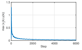
Figure 1: The consensus result of (5).

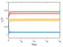
Figure 2: The trajectories of $y_{i}(k)$ by (5).

Theorem 2 is verified as follows. If the intersection of optimal solution sets to each agent is empty, then there is a graph sequence such that (5) is not convergent. The result is very similar to Fig. 2, and is omitted here. Consider all agents being with the same $q_{i}$, and then $\bigcap_{i\in\mathcal{V}}X_{i}^{*}\not=\emptyset$. Fig. 3 shows the trajectories of $y_{i}(k)$, where the network $\mathcal{G}(k)$ switches freely within four strongly connected graphs. The result indicates the convergence of (5) in this case.

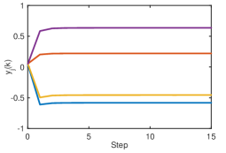
Figure 3: The trajectories of $y_{i}(k)$ with $\bigcap_{i\in\mathcal{V}}X_{i}^{*}\not=\emptyset$.

In the following, we demonstrate convergence results of (5) under periodic and quasi-periodic graph sequences. We generate each entry of $q_{i}$ by a uniform distribution over $[-2,2]$, and three graphs $\mathcal{G}_{A_{1}}$, $\mathcal{G}_{A_{2}}$ and $\mathcal{G}_{A_{3}}$, where $\mathcal{G}_{A_{1}}\cup\mathcal{G}_{A_{2}}$ is strongly connected. Consider the graph sequence given by

$$\mathcal{G}_{A_{1}}\rightarrow\mathcal{G}_{A_{2}}\rightarrow\mathcal{G}_{A_{3}}\rightarrow\mathcal{G}_{A_{1}}\rightarrow\mathcal{G}_{A_{2}}\rightarrow\mathcal{G}_{A_{3}}\rightarrow\cdots.$$

By the centralized projected gradient algorithm, we compute the optimal solution $x^{*}$ to (10). Then we employ (5) for this problem, and plot the trajectory of $\max_{i\in\mathcal{V}}|x_{i}(k)-x^{*}|$ in Fig. 4. In this case, (5) achieves a solution to (10) due to $\lim_{k\to\infty}|x_{i}(k)-x^{*}|=0$.

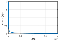
Figure 4: The convergence result of algorithm (5) under a periodic graph sequence.

We discuss the case of quasi-periodic graph sequences. To be specific, $\mathcal{G}(k)$ switches between $\mathcal{G}_{A_{1}}\rightarrow\mathcal{G}_{A_{2}}\rightarrow\mathcal{G}_{A_{3}}$ and $\mathcal{G}_{A_{3}}\rightarrow\mathcal{G}_{A_{2}}\rightarrow\mathcal{G}_{A_{1}}$ at each time interval $[3t,3(t+1))$. By (21), we construct a graph sequence such that (5) is not convergent, and show the result in Fig. 5.

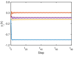
Figure 5: The convergence result of (5) under a quasi-periodic graph sequence.

Finally, we consider $\mathcal{G}(k)$ switching freely between $\mathcal{G}_{A_{1}}\rightarrow\mathcal{G}_{A_{2}}$ and $\mathcal{G}_{A_{2}}\rightarrow\mathcal{G}_{A_{1}}$ at each time interval $[2t,2(t+1))$. Fig. 6 shows the state trajectory of (5). The result indicates the convergence of (5) in this case. Figs. 5 and 6 imply the correctness of Theorem 4.

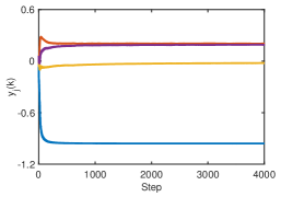
Figure 6: The convergence result of (5) under a quasi-periodic graph.

VII Conclusions

This paper aimed at investigating convergence properties of a distributed projected subgradient algorithm, where weight matrices of the time-varying communication network were only required to be row stochastic, i.e, the network might be weight-unbalanced. Firstly, it was proved that there generally existed a graph sequence such that the algorithm was not convergent if the network switched freely within finitely many general graphs. Then to guarantee the convergence of this algorithm for any uniformly strongly connected general graph sequence, it was provided a necessary and sufficient condition, i.e., the intersection of optimal solution sets to all local optimization problems was not empty. Following that, it was found that the algorithm was convergent under periodically switching general graph sequences, and optimized a weighted sum of local cost functions. Furthermore, the periodic condition was slightly relaxed by quasi-periodic graph sequences, and it was shown that the algorithm was always convergent for any quasi-periodic graph sequence if and only if the network switched between two graphs. Finally, numerical simulations were carried out for illustration.

References

- [1] S. Kar, J. M. F. Moura, and K. Ramanan, “Distributed parameter estimation in sensor networks: Nonlinear observation models and imperfect communication,” IEEE Transactions on Information Theory, vol. 58, no. 6, pp. 3575–3605, 2012.
- [2] D. K. Molzahn, F. Dörfler, H. Sandberg, S. H. Low, S. Chakrabarti, R. Baldick, and J. Lavaei, “A survey of distributed optimization and control algorithms for electric power systems,” IEEE Transactions on Smart Grid, vol. 8, no. 6, pp. 2941–2962, 2017.
- [3] S. Boyd, N. Parikh, E. Chu, B. Peleato, and J. Eckstein, “Distributed optimization and statistical learning via the alternating direction method of multipliers,” Foundations and Trends® in Machine Learning, vol. 3, no. 1, pp. 1–122, 2011.
- [4] A. Nedić and A. Ozdaglar, “Distributed subgradient methods for multi-agent optimization,” IEEE Transactions on Automatic Control, vol. 54, no. 1, pp. 48–61, 2009.
- [5] A. Nedić, A. Ozdaglar, and P. A. Parrilo, “Constrained consensus and optimization in multi-agent networks,” IEEE Transactions on Automatic Control, vol. 55, no. 4, pp. 922–938, 2010.
- [6] P. Lin, W. Ren, and Y. Song, “Distributed multi-agent optimization subject to nonidentical constraints and communication delays,” Automatica, vol. 65, pp. 120–131, 2016.
- [7] V. S. Mai and E. H. Abed, “Distributed optimization over directed graphs with row stochasticity and constraint regularity,” Automatica, vol. 102, pp. 94–104, 2019.
- [8] M. Zhu and S. Martínez, “On distributed convex optimization under inequality and equality constraints,” IEEE Transactions on Automatic Control, vol. 57, no. 1, pp. 151–164, 2011.
- [9] A. Cherukuri and J. Cortés, “Initialization-free distributed coordination for economic dispatch under varying loads and generator commitment,” Automatica, vol. 74, pp. 183–193, 2016.
- [10] X. Zeng, P. Yi, Y. Hong, and L. Xie, “Distributed continuous-time algorithms for nonsmooth extended monotropic optimization problems,” SIAM Journal on Control and Optimization, vol. 56, no. 6, pp. 3973–3993, 2018.
- [11] A. Nedić, A. Olshevsky, and M. G. Rabbat, “Network topology and communication-computation tradeoffs in decentralized optimization,” in Proceedings of the IEEE, 2018, pp. 953–976.
- [12] B. Gharesifard and J. Cortés, “Distributed continuous-time convex optimization on weight-balanced digraphs,” IEEE Transactions on Automatic Control, vol. 59, no. 3, pp. 781–786, 2013.
- [13] D. Yuan, D. W. Ho, and Y. Hong, “On convergence rate of distributed stochastic gradient algorithm for convex optimization with inequality constraints,” SIAM Journal on Control and optimization, vol. 54, no. 5, pp. 2872–2892, 2016.
- [14] Y. Lou, G. Shi, K. H. Johansson, and Y. Hong, “Approximate projected consensus for convex intersection computation: Convergence analysis and critical error angle,” IEEE Transactions on Automatic Control, vol. 59, no. 7, pp. 1722–1736, 2014.
- [15] A. Olshevsky and J. N. Tsitsiklis, “On the nonexistence of quadratic Lyapunov functions for consensus algorithms,” IEEE Transactions on Automatic Control, vol. 53, no. 11, pp. 2642–2645, 2008.
- [16] S. Pu, W. Shi, J. Xu, and A. Nedić, “Push-pull gradient methods for distributed optimization in networks,” IEEE Transactions on Automatic Control, vol. 66, no. 1, pp. 1–16, 2021.
- [17] K. I. Tsianos, S. Lawlor, and M. G. Rabbat, “Push-sum distributed dual averaging for convex optimization,” in 51st IEEE Conference on Decision and Control. Maui, HI, USA: IEEE, 2012, pp. 5453–5458.
- [18] K. I. Tsianos and M. G. Rabbat, “Distributed dual averaging for convex optimization under communication delays,” in American Control Conference. Montreal, QC, Canada: IEEE, 2012, pp. 1067–1072.
- [19] Y. Lou, Y. Hong, L. Xie, G. Shi, and K. H. Johansson, “Nash equilibrium computation in subnetwork zero-sum games with switching communications,” IEEE Transactions on Automatic Control, vol. 61, no. 10, pp. 2920–2935, 2015.
- [20] S. Liu, Z. Qiu, and L. Xie, “Convergence rate analysis of distributed optimization with projected subgradient algorithm,” Automatica, vol. 83, pp. 162–169, 2017.
- [21] R. A. Horn and C. R. Johnson, Matrix Analysis. Cambridge university press, 2012.
- [22] S. Liang, L. Wang, and G. Yin, “Dual averaging push for distributed convex optimization over time-varying directed graph,” IEEE Transactions on Automatic Control, vol. 65, no. 4, pp. 1785–1791, 2019.
- [23] Z. Qiu, S. Liu, and L. Xie, “Distributed constrained optimal consensus of multi-agent systems,” Automatica, vol. 68, pp. 209–215, 2016.
- [24] A. Nedić, A. Olshevsky, and W. Shi, “Achieving geometric convergence for distributed optimization over time-varying graphs,” SIAM Journal on Optimization, vol. 27, no. 4, pp. 2597–2633, 2017.
- [25] G. Shi and K. H. Johansson, “Robust consensus for continuous-time multiagent dynamics,” SIAM Journal on Control and Optimization, vol. 51, no. 5, pp. 3673–3691, 2013.
- [26] L. Wang and L. Guo, “Robust consensus and soft control of multi-agent systems with noises,” Journal of Systems Science and Complexity, vol. 21, no. 3, pp. 406–415, 2008.
- [27] G. Shi, K. H. Johansson, and Y. Hong, “Reaching an optimal consensus: Dynamical systems that compute intersections of convex sets,” IEEE Transactions on Automatic Control, vol. 58, no. 3, pp. 610–622, 2012.
- [28] I. Lobel and A. Ozdaglar, “Distributed subgradient methods for convex optimization over random networks,” IEEE Transactions on Automatic Control, vol. 56, no. 6, pp. 1291–1306, 2010.
- [29] J. Hajnal and M. S. Bartlett, “Weak ergodicity in non-homogeneous markov chains,” Mathematical Proceedings of the Cambridge Philosophical Society, vol. 54, no. 2, pp. 233–246, 1958.
- [30] B. T. Polyak, Introduction to Optimization. New York, NY, USA: Optimization Software, Inc., 1987.