Bidirectional group random walk based network embedding for asymmetric proximity

Abstract

Network embedding aims to represent a network into a low dimensional space where the network structural information and inherent properties are maximumly preserved. Random walk based network embedding methods such as DeepWalk and node2vec have shown outstanding performance in the aspect of preserving the network topological structure. However, these approaches either predict the distribution of a node’s neighbors in both direction together, which makes them unable to capture any asymmetric relationship in a network; or preserve asymmetric relationship in only one direction and hence lose the one in another direction. To address these limitations, we propose bidirectional group random walk based network embedding method (BiGRW), which treats the distributions of a node’s neighbors in the forward and backward direction in random walks as two different asymmetric network structural information. The basic idea of BiGRW is to learn a representation for each node that is useful to predict its distribution of neighbors in the forward and backward direction separately. Apart from that, a novel random walk sampling strategy is proposed with a parameter $\alpha$ to flexibly control the trade-off between breadth-first sampling (BFS) and depth-first sampling (DFS). To learn representations from node attributes, we design an attributed version of BiGRW (BiGRW-AT). Experimental results on several benchmark datasets demonstrate that the proposed methods significantly outperform the state-of-the-art plain and attributed network embedding methods on tasks of node classification and clustering.

1 Introduction

Networks are ubiquitous in various real-world scenarios, e.g., social networks, citation networks, biology networks. Mining useful information in networks can benefit lots of real-word applications, such as node classificationJi et al. (2011); Li et al. (2020), node clusteringSun et al. (2009) and link predictionGao et al. (2011), and thus has drawn wide attention in both academia and industry. Network embedding provides an effective and efficient way to mine information in networks. Generally, it aims to represent a network into a low dimensional vector space where the topological structure and inherent properties of the network can be preserved as much as possible.

One of the most common challenges of network embedding comes from how to define the proximity between two vertexes. The first-order and second-order proximities are two common similarities in the network embedding literatureCai et al. (2018); Goyal and Ferrara (2018). The first-order proximity indicates that nodes connected by each other should be similar and hence can be considered as a proximity to preserve local network structure. However, the observed links often only cover a small portion on real-world networks. Hence, the first-order proximity is not sufficient to preserve the network structure. The second-order proximity is an important complement, which assumes that nodes with similar distribution of neighbors should also have similar representations. How to preserve the pre-defined proximity is another challenge in network embedding. Some earlier work like LLEBelkin and Niyogi (2001) and LERoweis and Saul (2000) preserve the first-order proximity by factorizing graph Laplacian eigenmaps. However, they suffer from both computational and statistical drawbacks. Another set of studies (Ahmed et al. (2013); Cao et al. (2015); Ou et al. (2016)) try to directly factorize the node proximity matrix. But these methods are still not scalable for real-world networks due to high time complexity.

Random walk based network embedding methods such as DeepWalk Perozzi et al. (2014) and node2vec Grover and Leskovec (2016) have shown outstanding performance in the field of preserving network topological structure. In general, they adopt random walk sampling to generate neighbors for nodes in a network, which allow them to explore deeper vertices, then maximize the probability of observing the sampled neighbors for nodes conditioned on representations using SkipGramMikolov et al. (2013) model. In this way, the second-order proximity is implicitly preserved. Both of DeepWalk and Node2vec have an assumption that a source vertex and target vertex have a symmetric effect over each other. However, this assumption often doesn’t hold true in real world applications. For example, in social network like Twitter, supposing that user $A$ follows user $B$, the importance of $B$ for $A$ can’t simply equal to that of $A$ for $B$. Obviously, those who a user follows and his followers are two kinds of different asymmetric relational information. Generally, We observe that neighbors of a node can be divided into two categories: neighbors in the forward direction of random walks or neighbors in the backward direction. The former refers to vertices that can be accessed in random walks starting from that vertex, while the later refers to vertices from which can access that vertex in random walks. For directed networks, the structure of neighbors of a node in the forward and backward direction is usually different. For undirected networks, though a node have same neighbors in the forward and backward direction, they differ in the importance of each neighbor. Hence, in both directed and undirected networks, the distributions of these two kinds of neighbors are different and represent two kinds of asymmetric structural information. Figure 1 illustrates the difference between the distributions of forward and backward 1-hop neighbors in both directed and undirected networks. It can be seen that the probability of $A$ arriving at $C$ does not equal to that of $C$ arriving at $A$ due to their asymmetric local structure. However, both of DeepWalk and node2vec don’t distinguish a node’s neighbors by the forward and backward direction. Instead, they predict the distribution of neighbors in both direction together for each node conditioned on its embedding, which makes the occurrence number of vertex pair $(A,C)$ and $(C,A)$ be same. Hence, they can not capture any asymmetric relationship in a network.

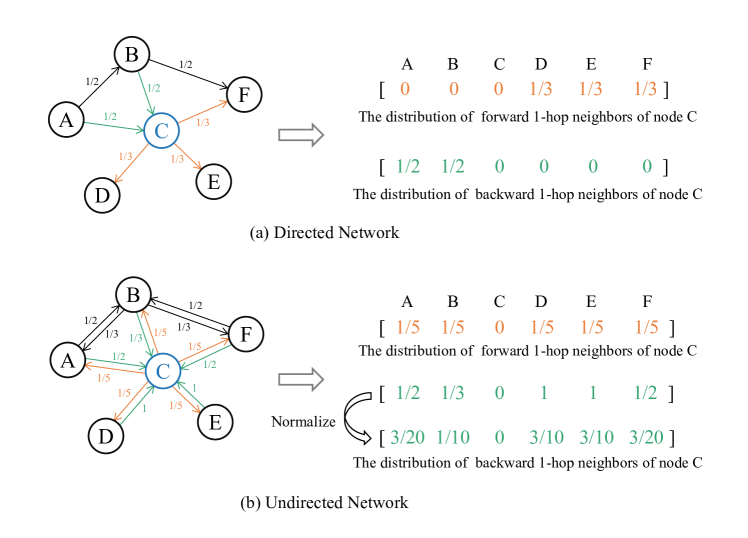
Figure 1: The distributions of neighbors in the forward and backward directions for directed and undirected networks.

Several researchers focus on preserving various asymmetric relationships in a network. For example, APPZhou et al. (2017) employs random walks on a network with restart and treats vertex pairs only in the forward direction as positive pairs, which allow it able to preserve the asymmetric relationship in the forward direction. GraRepCao et al. (2015) preserves the asymmetric relationship in the backward direction under matrix factorization framework. However, these approaches only consider asymmetric relationship in either forward or backward direction, and hence would lose the asymmetric relationship in another direction. Finding that the distributions of a node’s neighbors in the forward and backward direction are two kinds of asymmetric structural information, we propose learning a representation for each vertex to predict the distributions of its neighbors in the forward and backward direction separately. To our best knowledge, this is the first attempt to preserve asymmetric structural information in both forward and backward direction of random walks.

Observing that neighbors with different distances may have different significance, we propose weighted average of $1$-$k$ steps transitivity proximity ($k$-WAT) and give its mathematical definition in section 3. Due to the high-efficiency of random walks in terms of time and space complexityGrover and Leskovec (2016), we design a group random walk sampling strategy to implicitly preserve the proposed $k$-WAT proximity. Specifically, we divide neighbors into different groups according to the hops between two nodes. For example, given two random walk sequences: $u_{1}\rightarrow u_{4}\rightarrow u_{3}\rightarrow u_{2}$ and $u_{1}\rightarrow u_{2}$, $u_{2}$ is a 3-hop and 1-hop neighbor of $u_{1}$ in the former and later sequence respectively. At each random walk, we randomly choose the group of $l$-hop $(l\leq k)$ with the probability proportional to $\alpha^{l}$. The variation coefficient $\alpha$ actually controls a trade-off between BFS and DFS. Section 3 details the group random walk sampling strategy. Intuitively, small $\alpha$ would inspire walks to search towards nodes that are highly interconnected with the starting node and hence can benefit capturing community structure. On the contrary, large $\alpha$ would encourage walks to explore neighbors with longer distances and can help capture structural equivalence. Structural equivalence refers to that nodes having similar structural roles such as bridges or hubs in a network should have similar representations. Real-world networks often involve both of community structure and structural equivalence, though, their impact may vary with specific applications. Our method can flexibly control the trade-off between preserving community structure and structural equivalence based on specific cases.

Attributed network embedding has attracted wide attention in recent years. The idea is to learn low dimensional node representations that preserve both the network topological structure and attributes. The network attributes often contain some valuable information and can be helpful for some applications. Various approaches (e.g., TADWYang et al. (2015), GCNKipf and Welling (2016a), GraphSAGEHamilton et al. (2017)) have been proposed for attributed networks. However, since attribute information is usually associated with specific tasks, representations that preserve node attributes can not be generalized across different applications and the improvements of attributed network embedding approaches highly rely on the quality and relevance of attributes. In addition, the attribute information is often missing in real-world networks, which makes attributed network embedding methods hard to generalize. Despite these limitations, attributed network embedding approaches might have better performance for applications where high-quality and relevant attributes are available. Therefore, we design an attributed version of BiGRW (BiGRW-AT) to learn representations from node attributes. The basic idea is to obtain the target vector for each node from its attributes. The experimental results demonstrate that our method is superior to the existing attributed network embedding methods on both node classification and clustering.

To summarize, the main contributions of this paper are as follow:

• We propose a novel unsupervised network embedding model called BiGRW, which can effectively capture asymmetric structural information in both forward and backward direction of random walks. We also design an attributed version of BiGRW (BiGRW-AT) to learn representations from attribute information.

• We propose a novel proximity called $k$-WAT and design a group random walk algorithm via SkipGram model to implicitly preserve the proposed proximity with a parameter $\alpha$ to control the trade-off between BFS and DFS.

• We conduct experiments on several benchmark datasets. Experimental results demonstrate that our methods significantly outperform the existing unsupervised network embedding methods on the tasks of node classification and clustering.

The rest of this paper is organized as follow. In Section 2, we briefly introduce related work on network embedding. In Section 3, we present a mathematical definition of $k$-WAT proximity and detail the algorithm of our method. We present the experimental setting and results in Section 4 and conclude the paper in Section 5.

2 Related works

2.1 Plain network embedding

Plain network embedding focuses on learning node representations by preserving the network topological structure. Various approaches have been proposed. These approaches can be roughly divided into matrix factorization based methods and deep learning based methods.

Matrix factorization based network embedding methods aim to learn node embedding by factorizing the network property matrix(e.g., node proximity matrix). For example, Ahmed et al. (2013) propose decomposing the adjacency matrix of a network to preserve the first order proximity. HOPEOu et al. (2016) uses generalized Singular Value Decomposition(SVD) to preserve various higher order proximities such as Katz Index and Rooted Page Rank. GraRepCao et al. (2015) factorizes the $k$-step probability transition matrix by SVD to obtain embedding for different $k$ separately and concatenates them together after training.

The methods based on the deep learning framework can be further divided into two categories according to whether random walk is adopted to sample node sequences from a network. The basic idea of random walk based approaches is to generate a node’s neighbors by random walk sampling and then maximize the probability of observing the neighbors of a node conditioned on its representation. For example, DeepWalkPerozzi et al. (2014) firstly applies truncated random walks to sample node sequences and learns node representations from the sequences by using SkipGram model. Node2vecGrover and Leskovec (2016) extends DeepWalk by proposing a more flexible sampling strategy with two parameters to control the trade-off between BFS and DFS. The second class of deep learning based network embedding methods directly adopt deep learning framework to preserve network topological structure without random walks. For example, LINETang et al. (2015) treats immediately connected vertices as neighbours when defining the second order proximity. It preserves the first and second order proximities separately and concatenates them after training. SDNEWang et al. (2016) preserves the second order proximity by reconstructing the adjacency matrix under the encoder-decoder framework, and in the meantime minimize the difference between hidden representations of connected nodes. Other examples in this category include Cao et al. (2016); Chen et al. (2018); Li et al. (2016).

2.2 Attributed network embedding

Attributed network embedding aims to learn node representations from both the network topological structure and node attributes. A wide variety of attributed network embedding approaches have been proposed in recent years. Generally, they can be roughly divided into three categories. The first category is based on the matrix factorization framework. For example, TADWYang et al. (2015) employs matrix factorization to combine the network topological structure and node attributes. AANEHuang et al. (2017) decomposes the attribute affinity matrix with a penalty of embedding difference between connected nodes. Other examples in this category contain Bandyopadhyay et al. (2019); Pan et al. (2020); Yang et al. (2019).

The second category applies auto-encoder framework. For example, DANEGao and Huang (2018) uses two auto-encoders to preserve the network topological structure and node attributes respectively with a modality strategy to combine them. ANRLZhang et al. (2018) employs an auto-encoder with node attributes as input to reconstruct the attributes and in the meanwhile predicts the neighborhood. Other examples using the auto-encoder framework include Fan et al. (2021); Li et al. (2021); Liu et al. (2018, 2019).

The third category is built upon graph convolutional networks, where node attributes are propagated along network edges. For example, GCNKipf and Welling (2016a) employs the graph convolution operation among the immediate neighbors of each node to obtain the semi-supervised network embedding. GraphSAGEHamilton et al. (2017) extends GCN with several aggregators to aggregate node attributes from a sampled set of immediate neighbors. GAE and VGAEKipf and Welling (2016b) use GCN to learn node representations that are helpful to reconstruct the network adjacency matrix. Other examples in this category include Chiang et al. (2019); Pei et al. (2020); Veličković et al. (2017)

3 The proposed approach

In this section, we present the proposed approach. Table 1 lists the main symbols used in this paper.

Table 1: Terms and Notations

Symbol	Meaning
$V$	the set of vertices
$W^{(k)}$	the $k$-WAT matrix
$W_{ij}^{(k)}$	the element at i-th row and j-th column of $W^{(k)}$
$\tilde{W}_{i\cdot}^{(k)}$, $\tilde{W}_{\cdot i}^{(k)}$	the normalized i-th row and i-th column of $W^{(k)}$ respectively
$\tilde{W}_{i\cdot}^{(k)}(j)$, $\tilde{W}_{\cdot i}^{(k)}(j)$	the j-th element of $\tilde{W}_{i\cdot}^{(k)}$ and $\tilde{W}_{\cdot i}^{(k)}$ respectively
$S_{i}$	the embedding source vector for vertex $v_{i}$
$T_{i}^{(f)}$, $T_{i}^{(b)}$	the forward and backward target vector for vertex $v_{i}$ respectively
$X_{i}$	the features of vertex $v_{i}$
$H_{f}$,$H_{b}$	the forward and backward weight matrix respectively

3.1 Model overview

Figure 2 shows the overview of the proposed BiGRW and BiGRW-AT. Specifically, we first simulate group random walks on the network to obtain positive node pairs. The starting node and ending node at each walk sequence are treated as a positive node node. For per node pair, the starting node and ending node are considered as the source node and target node respectively in the forward direction. The situation is opposite in the backward direction. We then pass the positive node pairs to the SkipGram model to update the representations of the corresponding nodes. Negative sampling is adopted at this stage. For BiGRW-AT, the target vectors for each direction is modified as the product of the node feature matrix and a trainable weight matrix.

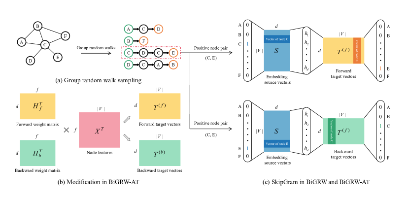
Figure 2: The overview of BiGRW and BiGRW-AT. For positive node pair $(C,E)$, the starting node $C$ and the ending node $E$ in a random walk sentence are treated as the source node and target node respectively in the forward direction, which is opposite in the backward direction. Both share the same embedding source vectors $S$. For BiGRW-AT, the target vectors for each direction is modified as the product of the node feature matrix and a trainable weight matrix.

3.2 The forward and backward $k$-WAT proximities

The second-order proximity assumes that vertices with similar distributions of neighbors are similar to each other. We find that a node’s neighbors can be divided into two categories: neighbors in the forward direction of random walks or neighbors in the backward direction. The former refers to vertices that can be accessed from that vertex in random walks, while the later refers to vertices from which can access that vertex. Apart from that, neighbors with different distances may have different significance. Based on these two observations, we define the forward and backward $k$-WAT distributions of a node’s neighbors in Definition 1.

Definition 1

($k$-WAT matrix) Let $A$ be the probability transition matrix in a random walk, $A_{ij}$ is the transition probability from vertex $i$ to vertex $j$ with one step. We observe that $A^{k}$ is the k-step probability transition matrix and $A_{ij}^{k}$ is exactly the transition probability from vertex $i$ to vertex $j$ after $k$ steps. The $k$-WAT matrix is defined as follow:

$$W^{(k)}=\alpha_{1}A^{1}+\alpha_{2}A^{2}+\cdots+\alpha_{k}A^{k}$$

where $\alpha_{k}$ is the weight for the group of k-hop , s.t., $\alpha_{1}+\alpha_{2}+\cdots+\alpha_{k}=1$. Specially, $\alpha_{l}=\frac{\alpha^{l}}{\sum_{i=1}^{k}\alpha^{i}}(l\leq k)$ in BiGRW, where $\alpha$ is the variation coefficient.

For vertex $v_{i}$, the forward $k$-WAT distribution of its neighbors in the forward direction is defined as the normalized $i$-th row of $k$-WAT matrix $W^{(k)}$; while the $k$-WAT distribution of its neighbors in the backward direction is defined as the normalized $i$-th column of $W^{(k)}$. Naturally, the forward and backward $k$-WAT proximities can be defined as follow:

Definition 2

(Forward k-WAT proximity) The forward $k$-WAT proximity between vertex $v_{i}$ and $v_{j}$ is defined as the similarity of $\tilde{W}_{i\cdot}^{(k)}$ and $\tilde{W}_{j\cdot}^{(k)}$, where $\tilde{W}_{i\cdot}^{(k)}$ and $\tilde{W}_{j\cdot}^{(k)}$ are the the normalized i-th row and j-th row of $W^{(k)}$ respectively.

Definition 3

(Backward k-WAT proximity) The backward $k$-WAT proximity of $v_{i}$ and $v_{j}$ is defined as the similarity of $\tilde{W}_{\cdot i}^{(k)}$ and $\tilde{W}_{\cdot j}^{(k)}$, where $\tilde{W}_{\cdot i}^{(k)}$ and $\tilde{W}_{\cdot j}^{(k)}$ are the normalized i-th column and j-th column of $W^{(k)}$ respectively.

Obviously, the forward and backward $k$-WAT proximities are two kinds of asymmetric structural relationships. Thus we try to learn a representation for each node that is useful to predict the $k$-WAT distribution of its neighbors in the forward and backward direction separately.

3.3 Loss functions

Formally, let $p_{i}(\cdot)=(p_{i}(1),p_{i}(2),\cdots,p_{i}(|V|))$ denote the pre-defined $k$-WAT distribution of neighbors in the forward or backward direction for vertex $v_{i}$, $q_{i}(\cdot)=(q_{i}(1),q_{i}(2),\\ \cdots,q_{i}(|V|))$ denote the predicted distribution conditioned on the representation of vertex $v_{i}$. Note that $p_{i}(\cdot)$ is exactly $\tilde{W}_{i\cdot}^{(k)}$ for the forward direction, or $\tilde{W}_{\cdot i}^{(k)}$ for the backward direction. The term $q_{i}(j)$ for the forward direction is defined as:

$$q_{i}(j)=\frac{\exp(S_{i}\cdot T_{j}^{(f)})}{\sum_{k\in V}\exp(S_{i}\cdot T_{k}^{(f)})},$$

while $q_{i}(j)$ for the backward direction is defined as:

$$q_{i}(j)=\frac{\exp(S_{i}\cdot T_{j}^{(b)})}{\sum_{k\in V}\exp(S_{i}\cdot T_{k}^{(b)})},$$

where $S_{i}$ is the embedding source vector for vertex $v_{i}$, while $T_{i}^{(f)},T_{i}^{(b)}$ are the forward and backward target vectors for vertex $v_{i}$, respectively.

To preserve the corresponding proximity, we minimize the distance between $p_{i}(\cdot)$ and $q_{i}(\cdot)$ :

$$\mathcal{L}=\sum_{i\in V}d(p_{i}(\cdot),q_{i}(\cdot)),$$

where $d(\cdot,\cdot)$ is the distance measure between two distribution. Adopting KL-divergence as the distance measure and omitting some constants, we have :

$$\mathcal{L}_{f}=-\sum_{i}\sum_{j}\tilde{W}_{i\cdot}^{(k)}(j)\log q_{i}(j),$$

$$\mathcal{L}_{b}=-\sum_{i}\sum_{j}\tilde{W}_{\cdot i}^{(k)}(j)\log q_{i}(j),$$

where $\mathcal{L}_{f}$ and $\mathcal{L}_{b}$ are the objective functions for the forward direction and backward direction respectively.

3.4 Optimization via group random walk sampling

Due to the high-efficiency of random walks in terms of both time and space complexity, we propose a group random walk sampling strategy to implicitly optimize the above objective, where the probability of visiting vertex $v_{j}$ starting from vertex $v_{i}$ within walk steps $k$ is exactly the term $W_{ij}^{(k)}$. Algorithm 1 details the group random walk sampling process. For each walk, we randomly choose the walk length $l(l\leq k)$ with the probability proportional to $\alpha^{l}$ and then simulate a walk with steps $l$ to get a starting vertex $u$ and an ending vertex $v$. Note that $u$ and $v$ are treated as the source vertex and the target vertex respectively in the forward direction, which is opposite in the backward direction, i.e., $v$ is the source vertex and $u$ is the target vertex.

Applying group random walk sampling, the forward $k$-WAT proximity in a network can be preserved in the latent representation space by maximizing the probability of observing the neighbors in the forward direction. The backward $k$-WAT proximity can be preserved likewise. The objective functions for the forward and backward directions are modified as following:

$$\mathcal{L}_{f}=-\sum_{(i,j)\in\mathcal{S}}\log q_{i}(j),$$

$$\mathcal{L}_{b}=-\sum_{(i,j)\in\mathcal{S}}\log q_{j}(i),$$

where $\mathcal{S}$ is the sampling set of positive node pair, and $(i,j)\in\mathcal{S}$ indicates that a walk path starting from vertex $v_{i}$ and ending at vertex $v_{j}$ being sampled in random walks. Since summation over all inner product with each vertex in a network is computationally expensive, we adopt negative sampling method to improve training efficiency, which distinguishes the target nearby vertices for each vertex from other vertices using logistic regression. Using negative sampling, we obtain the final objective functions:

$$\mathcal{L}_{f}=-\sum_{(i,j)\in\mathcal{S}}\Big{(}\log\sigma(S_{i}\cdot T_{j}^{(f)})+\sum_{k=1}^{Q}E_{v_{k}\sim P_{n}}[\log\sigma(-S_{i}\cdot T_{v_{k}}^{(f)})]\Big{)},$$ (1)

$$\mathcal{L}_{b}=-\sum_{(i,j)\in\mathcal{S}}\Big{(}\log\sigma(S_{i}\cdot T_{j}^{(b)})\\ +\sum_{k=1}^{Q}E_{v_{k}\sim P_{n}}[\log\sigma(-S_{i}\cdot T_{v_{k}}^{(b)})]\Big{)},$$ (2)

where $Q$ is the number of negative nodes that are sampled for each positive node pair. $P_{n}$ is the noise distribution for drawing negative samples.

Input: $G(V,E,W)$, variation coefficient $\alpha$, largest walk steps $k$, number of iterations $I$, number of negative samples $Q$

Output: the embedding source vectors $S$, the forward target vectors $T^{(f)}$, and the backward target vectors $T^{(b)}$

1 Initialize:$S$, $T^{(f)}$, $T^{(b)}$;

2

3for epoch=1 to I do

4       $\mathcal{O}$ = Shuffle($V$);

5       for each $u\in\mathcal{O}$ do

6            

7            $l$ = SampleWalkLength($k$, $\alpha$);

8             $v$ = SampleEndPoint($G,u,l$);

9             $L_{f}=-\log\sigma(S_{u}\cdot T_{v}^{(f)})$;

10             $L_{b}=-\log\sigma(S_{v}\cdot T_{u}^{(b)})$;

11             $Loss=L_{f}+L_{b}$;

12             for j=1 to Q do

13                   $neg$=RandomUniform($V$);

14                   $L_{f}=-\log\sigma(-S_{u}\cdot T_{neg}^{(f)})$;

15                   $L_{b}=-\log\sigma(-S_{v}\cdot T_{neg}^{(b)})$;

16                   $Loss+=L_{f}+L_{b}$;

17                  

18             end for

19            UpdateByAdam($Loss$, $(S,T^{(f)},T^{(b)})$);

20            

21       end for

22      

23 end for

Algorithm 1 Training Algorithm for BiGRW

3.5 Attributed version of BiGRW

In order to capture the node attributes, we design an attributed version of BiGRW. The objective function remains the same as formula 1 and 2. The only difference lies in the target vectors $T\in\mathcal{R}^{|V|\times d}$, which is modified as the product of the node feature matrix $X\in\mathcal{R}^{|V|\times f}$ and a trainable weight matrix $H\in\mathcal{R}^{f\times d}$, i.e., $T=XH$. For the forward and backward target vector of vertex $v_{i}$, $T_{i}^{(f)}=X_{i}H_{f}$, $T_{i}^{(b)}=X_{i}H_{b}$, respectively.

3.6 Complex analysis

The time complexity of the proposed BiGRW model framework consists of the random walk sampling process and the optimization via SkipGram model.

We can generate a positive node pair by simulating a random walk of length $l\leq k$. Hence, the time complexity of random walk process is $\mathcal{O}(kI|V|)$, where $k$, $I$, $|V|$ is the largest walk steps, the number of iterations and the number of nodes, respectively. For each node pair, the complexity of calculating loss objective function is $\mathcal{O}(d^{2})$ for each direction, where $d$ is the embedding dimension. Therefore, the complexity of the SkipGram part in BiGRW is $\mathcal{O}(d^{2}IQ|V|)$, where $Q$ is the number of negative samples. For BiGRW-AT, the operation of calculating the target vector from node attributes requires extra $\mathcal{O}(df^{2})$ per vertex, where $f$ is the dimension of attributes.

In summary, the overall complexity of BiGRW and BiGRW-AT is $\mathcal{O}(kI|V|+d^{2}IQ|V|)$ and $\mathcal{O}(kI|V|+d^{2}IQ|V|+df^{2}IQ|V|)$, respectively. By ignoring the parameters $d$, $k$, $f$, $I$ and $Q$ which are often small constants, the complexity of the proposed BiGRW and BiGRW-AT can be equivalent to $\mathcal{O}(|V|)$, which is scaling linearly w.r.t. the number of nodes in the network. Hence, our proposed model is computationally efficient and can be well applied on large-scale networks with millions of nodes and above.

4 Experiments

In this paper, we conduct experiments on three benchmark networks and evaluate the performance of various network embedding methods on tasks of node classification, node clustering and visualization. The experimental results demonstrate that our proposed methods performs better than the baseline methods.

4.1 Experimental setup

4.1.1 Datasets

In order to evaluate the effectiveness of network embedding methods, we collect three benchmark datasets, including two citation networks and one social network. Table 2 summarizes the description about these networks.

• Cora and CiteSeerYang et al. (2015): They are citation networks of scientific publications, where nodes indicate academic publications, and each edge represents a citation relationship between two publications.

• BlogCatalogTang and Liu (2009): It’s a social network of online users, where nodes represent bloggers on the BlogCatalog website, and each edge corresponds to a relationship between two bloggers.

Table 2: Statistics of the real-world networks

Name	Citation Network		Social Network
	Cora	CiteSeer	BlogCatalog
Nodes	2708	3327	10312
Edges	5429	4732	333983
Labels	7	6	39
Attributes	1433	3703	-

4.1.2 Baseline methods

Since BiGRW mainly focuses on preserving the network topological structure, we firstly compare it with the existing plain network embedding methods that also preserve the network topological structure. These baseline approaches are presented as follow:

• DeepWalk/node2vecGrover and Leskovec (2016); Perozzi et al. (2014): These two approaches adopt random walks to sample node sequences and use SkipGram model to learn node representations from the sampled sequences. We use $p=1$,$q=1$ in node2vec for comparison.

• LINETang et al. (2015): it preserves the first-order and second-order proximities separately and concatenates them after training.

• GraRepCao et al. (2015): it factorizes the $k$-steps ($k=1,2,3,\cdots$) probability transition matrix by SVD separately and concatenates them together after training.

• HOPEOu et al. (2016): it preserves various higher order proximities such as Katz Index and Rooted Page Rank by using generalized SVD.

• SDNEWang et al. (2016): it preserves the second order proximity by reconstructing the adjacency matrix under the encoder-decoder framework, and in the meantime minimize the difference between hidden representations of connected nodes.

For scenarios where node attributes are available, we compare the attributed version of BiGRW (BiGRW-AT) with the following unsupervised attributed network embedding approaches.

• Auto-encoder: We use an auto-encoder to preserve the node attributes only as the baseline method.

• GAE and VGAEKipf and Welling (2016b): These two approaches employ graph convolutional networks (GCNs) to propagate node features along edges on a network and learn representations to reconstruct the network adjacent matrix.

• TADWYang et al. (2015): it jointly preserves the network topological structure and node attributes under the framework of matrix factorization.

• GraphSAGEHamilton et al. (2017): it extends GCN with several aggregators to aggregate node attributes from a sampled set of immediate neighbors. We use its unsupervised version with mean-based aggregators.

• DANEGao and Huang (2018):it uses two auto-encoder to preserve the structural and attributed information respectively, and employs a cross modality strategy to combine the topological sturcture and attributes.

4.1.3 Parameters and reproducibility

All the methods are implemented in Pytorch. For all the baseline methods except Auto-encoder, we use the implementations provided by either the authors or open source projects on Github. We integrate all the implementations into an same framework where each model is evaluated using unified testing code after obtaining its embedding. For fairness, the final embedding dimension of all the models is set to 256 on Cora and Citeseer, 128 on BlogCatalog. For models that concatenate two vectors as the final embedding, each vector is set to 128 on Cora and Citeseer, 64 on BlogCatalog. For node2vec, the two important parameters are set as $p=1$ and $q=1$. For LINE, we concatenate the first-order and second-order representations to obtain the final embedding. For GraRep, the maximum step is set to 4. For GraphSAGE, we remove the rectified linear units (ReLU) in the output layer since we observe that this modification can benefit its performance in experiments. Other hyper-parameters are set as the default values provided in either the corresponding papers or open source projects. The major hyper-parameter settings for BiGRW and BiGRW-AT are summarized in Table 3.

Table 3: Major hyper-parameters in BiGRW and BiGRW-AT.

Methods	Dataset	Variation coefficient $\alpha$	Largest walk steps $k$	Embedding dimension $d$
BiGRW	Cora	1.25	5	256
	Citeseer	1.25	6	256
	BlogCatalog	0.75	5	128
BiGRW-AT	Cora	0.75	6	256
	Citeseer	0.5	6	256

4.2 Experimental results

4.2.1 Node classification

Node classification is one of the most common tasks to evaluate the effectiveness of node embedding in the literature. In the node classification setting where part of nodes in a network have already been attached one or more labels, the goal is to predict labels for the left nodes based on the representations. Specifically, we randomly sample 10 % to 90 % of the labeled nodes as training samples and the remaining nodes are used as testing samplings. We repeat this process 10 times and compute the average value of both $Micro\text{-}F_{1}$ and $Macro\text{-}F_{1}$. For all approaches, we adopt a one-vs-rest logistic regression implemented by Scikit-learn for classification.

Figure 3 shows the performance of plain network embedding methods on node classification. From the results, we can see that the proposed BiGRW has better performance than the baseline methods in all cases, which demonstrates the effectiveness of BiGRW in the aspect of preserving network topological structure. In addition, random walk based network embedding methods (DeepWalk/node2vec and BiGRW) perform relatively well on citation networks. Compared with DeepWalk/node2vec, BiGRW achieves a noticeable improvement in all cases. Our explanation is as follow. DeepWalk/node2vec predict neighbors of nodes in both direction together and hence they can’t preserve any asymmetric structural information. On the contrary, BiGRW distinguishes neighbors between the forward and backward directions. It predicts the distribution of neighbors in the forward and backward direction separately, which allow it to capture asymmetric topological structure in both direction. Apart from that, the parameter $\alpha$ in BiGRW makes it flexibly control the trade-off between capturing the community structure and structural equivalence. The poor performance of LINE on citation networks is possibly because it only treat immediately connected nodes as neighbors, which only cover a small proportion of nodes and hence are not sufficient to preserve the network structure.

We evaluate the performance of unsupervised attributed network embedding methods in node classification on Cora and Citeseer, where node attributes are available. Figure 4 shows the results. As one can see, the proposed BiGRW-AT significantly outperforms the unsupervised attributed network embedding baseline approaches on both Cora and Citeseer too. It demonstrates that the proposed bidirectional mechanism and group random walk sampling strategy remain effective when network attributes are incorporated.

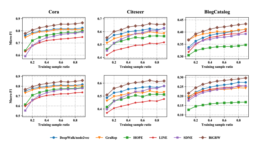
Figure 3: Node classification results of plain network embedding methods.

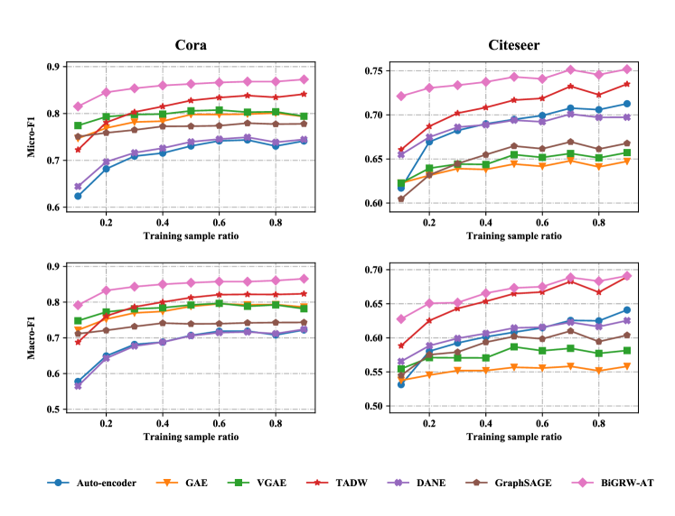
Figure 4: Node classification results of unsupervised attributed network embedding methods.

4.2.2 Node clustering

The task of node clustering aims to group similar node together. To further evaluate the effectiveness of network embedding, we conduct experiments on node clustering for each method after obtaining the node representations. Specifically, we apply the K-means clustering algorithm on the node embedding and evaluate the clustering results with the metrics of purity, normalized mutual information (NMI) and Matthews correlation coefficient (MCC). Table 4 shows the results of plain network embedding approaches. It can been seen that the proposed BiGRW is superior to the baseline approaches in all datasets. The results of unsupervised attributed network embedding approaches are shown in Table 5. As we can see, the proposed BiGRW-AT significantly outperforms all the baseline approaches in all cases. For example, in terms of NMI metric, BiGRW obtains 23.5% relative improvement compared with the best competitor (GAE) on Cora; on Citeseer, the relative improvement is 22.4% compared with the best competitor (DANE).

Table 4: Node clustering results of plain network embedding methods.

Methods	Cora			Citeseer			BlogCatalog
	Purity	NMI	MCC	Purity	NMI	MCC	Purity	NMI
DeepWalk/node2vec	0.6237	0.4414	0.3644	0.4435	0.2104	0.1263	0.4554	0.3476
LINE	0.5118	0.3092	0.1479	0.3312	0.0954	0.0346	0.4294	0.3303
GraRep	0.5679	0.3783	0.2771	0.3566	0.0940	0.0544	0.4445	0.3371
HOPE	0.3730	0.1406	0.0100	0.2585	0.0525	0.0305	0.3673	0.2936
SDNE	0.4306	0.2157	0.0720	0.3022	0.0817	0.0203	0.3663	0.2665
BiGRW	0.6680	0.4691	0.4041	0.4828	0.2609	0.1300	0.4754	0.3566

• As MCC is only applicable for binary classification, we don’t report the MCC result on BlogCatalog, where some of nodes have more than one labels.

Table 5: Node clustering results of unsupervised attributed network embedding methods.

Methods	Cora			Citeseer
	Purity	NMI	MCC	Purity	NMI	MCC
Auto-encoder	0.3951	0.1479	0.0992	0.4783	0.2276	0.1966
GAE	0.6518	0.4660	0.3556	0.5592	0.2617	0.2551
VGAE	0.6328	0.4054	0.3205	0.4094	0.1681	0.0959
DANE	0.6030	0.3580	0.2922	0.6513	0.3531	0.3560
GraphSAGE	0.5030	0.2742	0.1687	0.4837	0.2598	0.1555
TADW	0.6592	0.4591	0.3906	0.5580	0.2694	0.2268
BiGRW-AT	0.7441	0.5759	0.5469	0.7129	0.4321	0.4409

4.2.3 Parameter sensitivity

In order to evaluate the sensitivity of the three major hyper-parameters (i.e., variation coefficient $\alpha$, embedding dimension $d$ and largest walk steps $k$) in BiGRW, we conduct experiments on tasks of node classification and clustering on Cora. For variation coefficient $\alpha$, we fix $d=256$, $k=5$. For embedding dimension $d$, we fix $\alpha=1.25$, $k=5$. For largest walk steps $k$, we fix $\alpha=1.0$, $d=256$. Other hyper-parameters remain invariant.

Figure 5 and  6 show the results in node classification and clustering, respectively. As one can see, the performance of BiGRW on both tasks improves as $\alpha$ increases, and tends to saturate when $\alpha$ reaches around 1.25. The embedding dimension has relatively high impact on the performance of the method in node classification, but its influence is relatively small in node clustering. On both tasks, the trend of largest walk steps $k$ is quite similar with that of $\alpha$. Intuitively, larger $k$ allows walks to have larger search scope when defining neighbors, while $\alpha$ controls the proportion of neighbor groups of different hops, i.e., larger $\alpha$ would encourage walks to search nodes with longer distance as neighbors. Hence, larger $\alpha$ and $k$ would help BiGRW capture structure equivalence, which can be useful for node classification and clustering from the results on Cora.

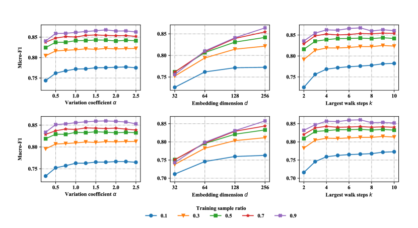
Figure 5: The parameter sensitivity results in node classification on Cora.

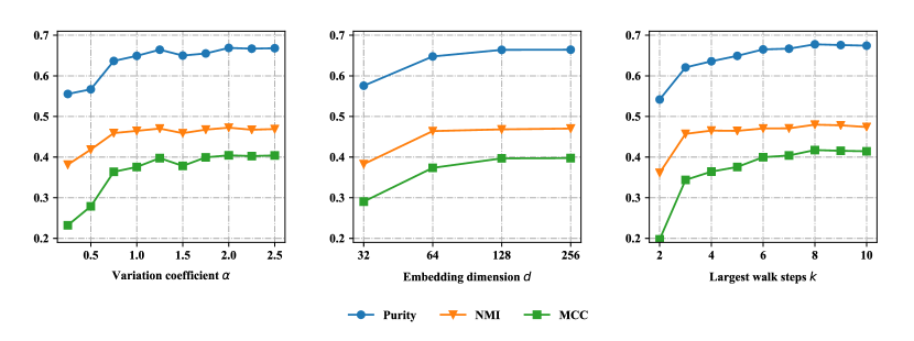
Figure 6: The parameter sensitivity results in node clustering on Cora.

4.2.4 Visualization

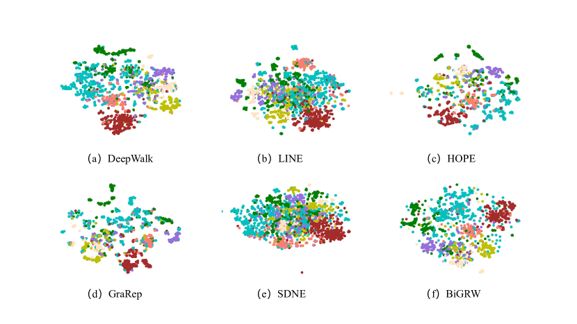
Figure 7: Visualizing results of the learned node representations on Cora. Each point indicates one paper and colors of nodes represent different publication divisions.

Finally, we visualize the learned node representations of unsupervised network embedding methods that focus on preserving network topological structure by using t-SNEVan der Maaten and Hinton (2008). Figure 7 shows the visualization results. BiGRW obtains relatively more compacted and separated clusters compared with the other baseline approaches, indicating the effectiveness of BiGRW in the aspect of preserving network structure again.

5 Conclusions

We have noticed that the distributions of a node’s neighbors in the forward and backward directions of random walks are two different asymmetric structural information. To capture asymmetric topological structure in both forward and backward directions, we proposed a novel network embedding model called BiGRW. The basic idea of BiGRW is to learn a representation for each node that is useful to predict its distribution of neighbors in the forward and backward direction separately. Apart from that, a novel random walk sampling strategy was proposed with a parameter $\alpha$ to flexibly control the trade-off between BFS and DFS. We also designed an attributed version of BiGRW to make it able to learn node representations from attributes. The experimental results demonstrate that BiGRW and its attributed version are significantly superior to the existing plain network embedding approaches and attributed network embedding approaches respectively in both node classification and clustering.

Our future research will focus on incorporating the bidirectional mechanism and group random walk sampling strategy into more complicated networks (e.g., heterogeneous networks and dynamic networks). We may also focus on designing more complex and effective mechanism to combine the network topological structure and node attributes.

References

- Ahmed et al. (2013) Ahmed A, Shervashidze N, Narayanamurthy S, Josifovski V, Smola AJ (2013) Distributed large-scale natural graph factorization. In: Proceedings of the 22nd international conference on World Wide Web, pp 37–48, DOI https://doi.org/10.1145/2488388.2488393
- Bandyopadhyay et al. (2019) Bandyopadhyay S, Lokesh N, Murty MN (2019) Outlier aware network embedding for attributed networks. In: Proceedings of the AAAI Conference on Artificial Intelligence, vol 33, pp 12–19, DOI https://doi.org/10.1609/aaai.v33i01.330112
- Belkin and Niyogi (2001) Belkin M, Niyogi P (2001) Laplacian eigenmaps and spectral techniques for embedding and clustering. Advances in neural information processing systems 14:585–591
- Cai et al. (2018) Cai H, Zheng VW, Chang KCC (2018) A comprehensive survey of graph embedding: Problems, techniques, and applications. IEEE Transactions on Knowledge and Data Engineering 30(9):1616–1637, DOI 10.1109/TKDE.2018.2807452
- Cao et al. (2015) Cao S, Lu W, Xu Q (2015) Grarep: Learning graph representations with global structural information. In: Proceedings of the 24th ACM international on conference on information and knowledge management, pp 891–900, DOI https://doi.org/10.1145/2806416.2806512
- Cao et al. (2016) Cao S, Lu W, Xu Q (2016) Deep neural networks for learning graph representations. In: Proceedings of the AAAI Conference on Artificial Intelligence, vol 30
- Chen et al. (2018) Chen H, Perozzi B, Hu Y, Skiena S (2018) Harp: Hierarchical representation learning for networks. In: Proceedings of the AAAI Conference on Artificial Intelligence, vol 32
- Chiang et al. (2019) Chiang WL, Liu X, Si S, Li Y, Bengio S, Hsieh CJ (2019) Cluster-gcn: An efficient algorithm for training deep and large graph convolutional networks. In: Proceedings of the 25th ACM SIGKDD International Conference on Knowledge Discovery & Data Mining, pp 257–266, DOI https://doi.org/10.1145/3292500.3330925
- Fan et al. (2021) Fan H, Zhong Y, Zeng G, Sun L (2021) Attributed network representation learning via improved graph attention with robust negative sampling. Applied Intelligence 51(1):416–426, DOI https://doi.org/10.1007/s10489-020-01825-x
- Gao and Huang (2018) Gao H, Huang H (2018) Deep attributed network embedding. In: Twenty-Seventh International Joint Conference on Artificial Intelligence (IJCAI))
- Gao et al. (2011) Gao S, Denoyer L, Gallinari P (2011) Temporal link prediction by integrating content and structure information. In: Proceedings of the 20th ACM international conference on Information and knowledge management, pp 1169–1174
- Goyal and Ferrara (2018) Goyal P, Ferrara E (2018) Graph embedding techniques, applications, and performance: A survey. Knowledge-Based Systems 151:78–94, DOI https://doi.org/10.1016/j.knosys.2018.03.022
- Grover and Leskovec (2016) Grover A, Leskovec J (2016) node2vec: Scalable feature learning for networks. In: Proceedings of the 22nd ACM SIGKDD international conference on Knowledge discovery and data mining, pp 855–864, DOI https://doi.org/10.1145/2939672.2939754
- Hamilton et al. (2017) Hamilton WL, Ying R, Leskovec J (2017) Inductive representation learning on large graphs. arXiv preprint arXiv:170602216
- Huang et al. (2017) Huang X, Li J, Hu X (2017) Accelerated attributed network embedding. In: Proceedings of the 2017 SIAM international conference on data mining, SIAM, pp 633–641
- Ji et al. (2011) Ji M, Han J, Danilevsky M (2011) Ranking-based classification of heterogeneous information networks. In: Proceedings of the 17th ACM SIGKDD international conference on Knowledge discovery and data mining, pp 1298–1306, DOI https://doi.org/10.1145/2020408.2020603
- Kipf and Welling (2016a) Kipf TN, Welling M (2016a) Semi-supervised classification with graph convolutional networks. arXiv preprint arXiv:160902907
- Kipf and Welling (2016b) Kipf TN, Welling M (2016b) Variational graph auto-encoders. arXiv preprint arXiv:161107308
- Li et al. (2016) Li J, Zhu J, Zhang B (2016) Discriminative deep random walk for network classification. In: Proceedings of the 54th Annual Meeting of the Association for Computational Linguistics (Volume 1: Long Papers), pp 1004–1013
- Li et al. (2020) Li K, Feng Y, Gao Y, Qiu J (2020) Hierarchical graph attention networks for semi-supervised node classification. Applied Intelligence 50(10):3441–3451, DOI https://doi.org/10.1007/s10489-020-01729-w
- Li et al. (2021) Li Z, Wang X, Li J, Zhang Q (2021) Deep attributed network representation learning of complex coupling and interaction. Knowledge-Based Systems 212:106618, DOI https://doi.org/10.1016/j.knosys.2020.106618
- Liu et al. (2018) Liu J, He Z, Wei L, Huang Y (2018) Content to node: Self-translation network embedding. In: Proceedings of the 24th ACM SIGKDD International Conference on Knowledge Discovery & Data Mining, pp 1794–1802, DOI https://doi.org/10.1145/3219819.3219988
- Liu et al. (2019) Liu J, Li N, He Z (2019) Network embedding with dual generation tasks. In: IJCAI, pp 5102–5108
- Van der Maaten and Hinton (2008) Van der Maaten L, Hinton G (2008) Visualizing data using t-sne. Journal of machine learning research 9(11)
- Mikolov et al. (2013) Mikolov T, Chen K, Corrado G, Dean J (2013) Efficient estimation of word representations in vector space. arXiv preprint arXiv:13013781
- Ou et al. (2016) Ou M, Cui P, Pei J, Zhang Z, Zhu W (2016) Asymmetric transitivity preserving graph embedding. In: Proceedings of the 22nd ACM SIGKDD international conference on Knowledge discovery and data mining, pp 1105–1114, DOI https://doi.org/10.1145/2939672.2939751
- Pan et al. (2020) Pan Y, Hu G, Qiu J, Zhang Y, Wang S, Shao D, Pan Z (2020) Flgai: a unified network embedding framework integrating multi-scale network structures and node attribute information. Applied Intelligence 50(11):3976–3989, DOI https://doi.org/10.1007/s10489-020-01780-7
- Pei et al. (2020) Pei H, Wei B, Chang KCC, Lei Y, Yang B (2020) Geom-gcn: Geometric graph convolutional networks. arXiv preprint arXiv:200205287
- Perozzi et al. (2014) Perozzi B, Al-Rfou R, Skiena S (2014) Deepwalk: Online learning of social representations. In: Proceedings of the 20th ACM SIGKDD international conference on Knowledge discovery and data mining, pp 701–710, DOI https://doi.org/10.1145/2623330.2623732
- Roweis and Saul (2000) Roweis ST, Saul LK (2000) Nonlinear dimensionality reduction by locally linear embedding. science 290(5500):2323–2326, DOI 10.1126/science.290.5500.2323
- Sun et al. (2009) Sun Y, Yu Y, Han J (2009) Ranking-based clustering of heterogeneous information networks with star network schema. In: Proceedings of the 15th ACM SIGKDD international conference on Knowledge discovery and data mining, pp 797–806, DOI https://doi.org/10.1145/1557019.1557107
- Tang et al. (2015) Tang J, Qu M, Wang M, Zhang M, Yan J, Mei Q (2015) Line: Large-scale information network embedding. In: Proceedings of the 24th international conference on world wide web, pp 1067–1077, DOI https://doi.org/10.1145/2736277.2741093
- Tang and Liu (2009) Tang L, Liu H (2009) Relational learning via latent social dimensions. In: Proceedings of the 15th ACM SIGKDD international conference on Knowledge discovery and data mining, pp 817–826, DOI https://doi.org/10.1145/1557019.1557109
- Veličković et al. (2017) Veličković P, Cucurull G, Casanova A, Romero A, Lio P, Bengio Y (2017) Graph attention networks. arXiv preprint arXiv:171010903
- Wang et al. (2016) Wang D, Cui P, Zhu W (2016) Structural deep network embedding. In: Proceedings of the 22nd ACM SIGKDD international conference on Knowledge discovery and data mining, pp 1225–1234, DOI https://doi.org/10.1145/2939672.2939753
- Yang et al. (2015) Yang C, Liu Z, Zhao D, Sun M, Chang EY (2015) Network representation learning with rich text information. In: IJCAI, vol 2015, pp 2111–2117
- Yang et al. (2019) Yang H, Pan S, Chen L, Zhou C, Zhang P (2019) Low-bit quantization for attributed network representation learning. In: IJCAI International Joint Conference on Artificial Intelligence
- Zhang et al. (2018) Zhang Z, Yang H, Bu J, Zhou S, Yu P, Zhang J, Ester M, Wang C (2018) Anrl: Attributed network representation learning via deep neural networks. In: IJCAI, vol 18, pp 3155–3161
- Zhou et al. (2017) Zhou C, Liu Y, Liu X, Liu Z, Gao J (2017) Scalable graph embedding for asymmetric proximity. In: Proceedings of the Thirty-First AAAI Conference on Artificial Intelligence, pp 2942–2948