A concise introduction to molecular dynamics simulation: Theory and programming

Abstract

We provided a concise and self-contained introduction to molecular dynamics (MD) simulation, which involves a body of fundamentals needed for all MD users. The associated computer code, simulating a gas of classical particles interacting via the Lennard-Jones pairwise potential, was also written in Python programming language in both top-down and function-based designs.

Keywords Molecular dynamics simulation $\cdot$ Classical particles $\cdot$ Lennard-Jones potential $\cdot$ Python programming language

Developed originally by Alder and Wainwright in the 1950s [1], and began to gain extensive attention in the mid-1970s concurrent with the advent of powerful computers, molecular dynamics (MD) methods have long been considered as orthodox means for simulating matter at molecular scales, continuing to excite the ardor of researchers with new problems, also from students new to molecular theory as well [2]. The very essence of MD, simply, is to solve numerically the $N$-body problem of classical mechanics—indeed, solving differential equations is what happens in all physics: Einstein field equations [3] in general relativity [4]; Schrödinger equation in quantum mechanics [5]; and Newton’s equations of motion in classical mechanics. At present, the importance of such a many-body problem arises from attempts to relate collective behaviors of many-body systems to the associated single-particle dynamics. MD simulation is indeed the modern realization of an old, deterministic, and mechanical interpretation of Nature in the sense that the behavior of the system could be exactly computed if initial conditions, namely positions, velocities, and accelerations of the constituent particles of that system are known [6]. It has also contributed to much of our understanding of systems out of equilibrium for which, theory, particularly statistical mechanics [7], has little to say [8].

Not only as a capable scientific method deployed to do research in applied areas of science and technology, such as drug discovery [9], biochemistry of diseases [10], etc., MD has also been exploited as an educational tool in a number of university courses including computational physics, chemistry, materials science, and biology.

The present work has been devoted to providing a brief, comprehensive, and self-contained overview of MD simulation. Indeed, compared to other topics such as numerical integration or solving differential equations, along with which MD is taught during one semester, the latter requires a dramatically larger amount of educational time due to being inherently more sophisticated and time-consuming. Here, we present a core of fundamentals that should be common to all users of MD. This introduction has been restricted to the simulation of a many-body system, in thermodynamic equilibrium, and composed of Lennard-Jones [11] atoms as hard spheres. The related computer code was also written in Python language in top-down as well as function-based programming styles. Quantum effects (as in ab initio MD [12, 13, 14]), multibody interactions (such as Axilrod-Teller three-body potential [15]), and simulating nonequilibrium processes [16] have not been discussed here. Previous exposure to classical and statistical mechanics, as well as programming in Python [17], C [18], or Fortran [19], could also be very useful.

1 Primitive concepts

System is defined as the portion (or subset) of the physical universe on which we concentrate. To investigate the behavior of the system, one needs ways to assign numerical values either to the state or to functions of that state. This assignment is called an observable. As an illustration, the ideal gas law, $PV=Nk_{B}T$, is a relation among the observables pressure $P$, volume $V$, number of particles $N$, and equilibrium temperature $T$ ($k_{B}$ being the Boltzmann constant). The state of the system can be manipulated or changed via interactions with its environment. The system and its immediate environment are separated via system’s boundary, which constrains system-environment interactions. Here, by system, we solely mean isolated system the boundary of which does not allow the exchange (entry or exit) of matter and energy with the surroundings.

1.1 MD is not a model

To establish connection between measurable outputs and controlled inputs is the goal of theoretical works. In theory, complicated interactions among state variables are entirely or partially decoupled in order for observable outputs to be computed. A model is indeed a scheme to decouple and eliminate interactions with negligible or no impact on the observables of interest. As a result, a model is simpler than the original system, having then access to fewer states, and vice versa, a model has access to some states which are not available to the system it imitates. A simulation, in contrast, is more complicated than the original system and can accordingly reach more states. However, the original system should not be considered as a model of the simulation at all.

1.2 MD simulations are computer experiments

Controversial arguments have so far arisen over the query of whether computer simulations like MD are theories or experiments. The theory side believe that simulations are not experiments, because they are as such pure calculations and no measurement is done on real systems during a computer simulation. The experiment side, on the other hand, argue that simulations are experiments because their results (i) are used to test theories, (ii) are reproducible, and (iii) are statistically error-prone. Indeed, the latter interpretation is widely accepted and pervaded the literature, and we likewise believe that MD simulations are computer experiments.

2 Fundamentals

2.1 Ergodic theorem

MD is a widespread class of computer simulations used in many areas of science particularly statistical mechanics, and involves two general forms including systems at equilibrium, as well as those away from equilibrium. The reliability of MD as such stems from the ergodic theorem introduced by Boltzmann. One, in fact, needs to be assured that the system to be simulated is ergodic, namely the associated time average and ensemble average are nearly the same, mainly based on the fact that an MD simulation produces a time evolution of that system. Most systems with realistic pairwise potentials fortunately seem to behave ergodically in two or more dimensions—one-dimensional systems should probably be viewed as suspects—in spite of the fact that only a few systems are indeed ergodic. Geometrically, a system is ergodic (or more realistically, quasiergodic) if the trajectory of its representative point (i.e., phase point) crosses any neighborhood of any point of the system’s phase space in the course of time. And Mathematically,

$$\langle A\rangle_{ens}=\frac{\int_{0}^{t_{tot}}dq{\hskip 1.42262pt}A(q){\hskip 1.42262pt}p(q)}{\int_{0}^{t_{tot}}dq{\hskip 1.42262pt}p(q)}\cong\lim_{t_{tot}\longrightarrow\infty}\frac{1}{t_{tot}}\int_{0}^{t_{tot}}dtA(q(t))=\langle A\rangle_{time},$$

meaning that if we wait long enough (i.e., $t_{tot}\longrightarrow\infty$), the ensemble average $\langle A\rangle_{ens}$ and the time average $\langle A\rangle_{time}$ of the thermodynamic observable $A$ of the system would be the same. Here $q$ is a microstate of the system, and might represent the positions and momenta of the constituent particles, and $p(q)$ is the associated probability distribution function. This is indeed based on this theorem that MD simulations are not reliable at very low temperatures due to lack of adequate vibrancy of the phase point—in this so-called low-temperature limit, we have in fact to deploy other methods such a phonon-dispersion calculations to derive the thermodynamics of the system.

In Monte Carlo (MC) methods [20], the other vast category of simulations in statistical mechanics, similar averaging is done, but on the phase space of the system, not on the created time-dependent trajectories as in MD. An inevitable error could therefore be assigned to either method: in MC, averaging should be done over the entire phase space, but we are only able to average over a limited number of samples; and in MD, we must wait infinitely, but it is not possible and averaging is practically done over limited durations of time. However, one could minimize such a kind of inherent error via optimally sampling the phase space (in MC), or by accurately estimating the characteristic timestep of the system (in MD).

2.2 Standard ensemble for MD

MC is based fundamentally on the Boltzmann weight factor $e^{-\beta\epsilon}$, where $\epsilon$ is the energy of a state of the system, and $\beta=1\big{/}k_{B}T$ is the inverse temperature of the surroundings. Accordingly, the standard ensemble for MC is the canonical ensemble due to the natural appearance of temperature in the Boltzmann factor, in which the total number $N$ of particles, the volume $V$, and the equilibrium temperature $T$ of the system are held fixed. Here, standard means only to pursue the relations existing in theory, and without applying any computational trick to obtain the desired result. By a similar reasoning, the standard ensemble for MD is however the microcanonical ensemble, in which, $N$, $V$, and the total energy $E$ are held fixed. In other words, by solely writing down the classical equations of motion in a computer language, a fixed total energy for the system of interest is then yielded. However, to simulate more realistic situations, one has to keep temperature or pressure of the system fixed, for which other statistical ensembles (say the canonical ensemble) must accordingly be used.

2.3 Interparticle interaction

One of the well-known interparticle potentials used in MD simulations is the Lennard-Jones (L-J) pair interaction, which is the most prevalent among other types of pairwise potentials (e.g., Morse [21], Yukawa [22], Coulomb, gravitational, and Buckingham [23]), and is considered as the archetype model for simple, yet-realistic interacting systems. In the L-J potential, the pairwise interaction is indeed of the van der Waals form, namely $r^{-6}$ with $r$ the interparticle distance, which describes attraction at long distances. This term could in fact be derived solely by using quantum mechanics. Adding repulsion at short distances via $r^{-12}$—according to the Pauli repulsion—then results in the L-J potential:

$$U_{LJ}(r)=-4\epsilon\bigg{[}\left(\frac{\sigma}{r}\right)^{6}-\left(\frac{\sigma}{r}\right)^{12}\bigg{]},$$ (1)

where $r=|{\bf{r}}_{1}-{\bf{r}}_{2}|$, ${\bf{r}}_{1}$ and ${\bf{r}}_{2}$ denote respectively the position vectors of particles 1 and 2, $\epsilon$ is the depth of the potential well (also referred to as the dispersion energy), and $\sigma$—often referred to as the particle size—is the distance at which $U_{LJ}$ vanishes (bold characters denote vectors). $r_{min}=2^{1/6}\sigma$ also corresponds with the minimum of the potential, as illustrated in Fig. 1

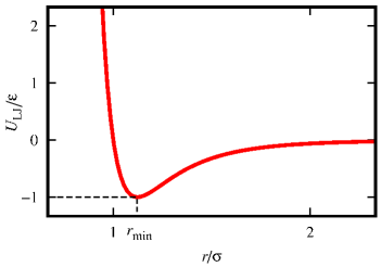
Figure 1: The Lennard-Jones pairwise potential ($U_{LJ}$) as a function of the distance $r$ between two interacting particles—rendered in Gnuplot (version 5.2) [24]. $r_{min}$, corresponding with the minimum value of the potential, takes place at $2^{1/6}\sigma$.

2.4 Long- and short-range interactions: The cutoff radius

Assume a universe of particles with a uniform distribution (Fig. 2) interacting via the pairwise potential $U$, which is proportional to $r^{-\alpha}$ ($\alpha>0$).

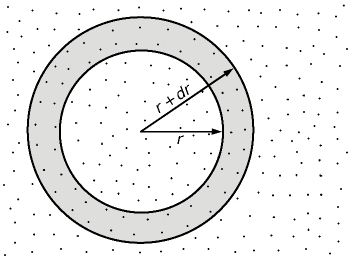
Figure 2: A universe of particles with a uniform distribution, and the two spheres with radii $r$ and $r+dr$ encompassing parts of the particles—rendered in GIMP (version 2.8.22) [25].

The question is that could it be reliable ignoring the collective effect of particles outside the sphere of radius $r_{c}$ on every point inside that sphere, and taking into account only the interactions of particles within that sphere, in order to merely reduce the computational cost?

The answer fundamentally depends on the value of $\alpha$. Assuming $\rho$ to be the particle density in the universe of Fig. 2, then

$$\Delta U(r)=\frac{\rho\hskip 2.84526pt4\pi r^{2}dr}{r^{\alpha}}\propto r^{2-\alpha}.$$

Now, if $\alpha<2$, then $\lim_{r\longrightarrow\infty}\Delta U=\infty$, and the interaction [i.e., $U(r)$] is said to be long-range. A clear illustration of this kind is the gravitational force for which $\alpha=1$, and therefore, $\Delta U(r)\propto r$ meaning that the farther the planet is from say Earth, the larger its potential energy effect on Earth. Accordingly, gravitational potential energy contributions of very distant celestial objects say at the edge of the galaxy, to our planet are considerably larger than that of the Sun, while the net contribution of their forces could be zero due to vector summation. Therefore, it is not reasonable to ignore particles outside the sphere if the pair interaction is gravitational.

In contrast, if $\alpha>2$, then $\lim_{r\longrightarrow\infty}\Delta U=0$, and the interaction is said to be short-range, such as the L-J potential. As a result, we can eliminate the particles outside a so-called cutoff radius ($r_{c}$), without loss of generality or reliability of calculations, in order to reduce the computational cost.

2.5 Choosing appropriate system of units: Making physical observables dimensionless

A given system of units, as such, is not more advantageous than other ones, and we, in theory, use a specific system of units only to speak in the same scientific language. However, in computer simulations particularly MD, choosing appropriate systems of units is of foremost importance. We, for example, cannot use the meter length scale in simulating nanoscale systems, or, it is not feasible using electron Volt energy scale when the process of interest is nuclear fusion in the Sun. In either case, one would get very large or very small numbers, and it is accordingly needed a huge amount of memory to save them, regardless of the rise of round-off errors.

Consider the simulation of a system composed of argon atoms interacting via the L-J potential. The mass $m_{A}$ of an argon atom, and the related L-J parameters, namely $\epsilon_{A}$ and $\sigma_{A}$, are tabulated in Table 1.

Table 1: The mass ($m_{A}$) of an argon atom, as well as the L-J parameters $\epsilon_{A}$, and $\sigma_{A}$ associated with a pair of argon atoms [26].

$m_{A}$ (kg)	$\epsilon_{A}$ (J)	$\sigma_{A}$ (m)
$6.7\times 10^{-26}$	$1.6\times 10^{-21}$	$3.4\times 10^{-10}$

As a result, $m^{*}\equiv m\big{/}m_{A}$, $E^{*}\equiv E\big{/}\epsilon_{A}$, and $r^{*}\equiv r\big{/}\sigma_{A}$ are respectively the dimensionless mass, energy, and distance, which form the reduced units. These dimensionless quantities, in fact, keep the MD simulation from generating very large or very small quantity values. Since the dimensions of mass, energy, and length are respectively M, ML²T^-2, and L, the characteristic time for simulating a system of argon atoms, using values of Table 1, is then obtained as

$$\sqrt{\mathrm{\frac{ML^{2}}{ML^{2}T^{-2}}}}={\mathrm{T}}\hskip 8.53581pt\Longrightarrow\hskip 8.53581pt\tau_{A}=\sigma_{A}\sqrt{\frac{m_{A}}{\epsilon_{A}}}\cong 10^{-12}\hskip 2.84526pt{\mathrm{s}}=1\hskip 2.84526pt{\mathrm{ps}}.$$

The dimensionless time is also then $t^{*}\equiv t\big{/}\tau_{A}$. This specific value, namely $\tau_{A}$, is indeed the characteristic timestep of a gas of argon atoms for which a logical relationship between any two consecutive events holds according to the principle of causality. For timesteps considerably larger than $\tau_{A}$, the simulation crashes because of loss of causality, while values much smaller than $\tau_{A}$ increase the computational cost and make accordingly the simulation dramatically slow. Timesteps of about $10^{-3,-4}\tau_{A}=10^{-15,-16}\hskip 2.84526pt{\mathrm{s}}$ are optimal for simulating systems at the scales of atoms and molecules.

The characteristic velocity is also $v_{A}=\sigma_{A}\big{/}\tau_{A}\cong 340\hskip 2.84526pt{\mathrm{m\big{/}s}}$, which is nearly the same velocity of sound. This, in fact, is reasonable because sound is nothing but the collisions of particles which propagate through a transmission medium. The dimensionless velocity is accordingly $v^{*}\equiv v\big{/}v_{A}$. The characters indicated by asterisks are called derived quantities due to being derived by fundamental quantities tabulated in Table 1.

As a consequence, property values generated by the computer code (i.e., outputs) are also evidently dimensionless, and one can re-attribute physical meanings to them by pursuing the reverse procedure. If, for example, the final time of the simulation is reported $10^{7}$, it means that

$$t^{*}=\frac{t}{\tau_{A}}=10^{7}\hskip 8.53581pt\Longrightarrow\hskip 8.53581ptt=10^{7}\hskip 2.84526pt\tau_{A}=10^{7}\times 10^{-16}\hskip 2.84526pt{\mathrm{s}}=1\hskip 2.84526pt{\mathrm{ns}}$$

3 Simulation preliminaries

3.1 Initialization

The first step in MD simulations at the level of programming is to assign initial values to each Cartesian component of atomic positions, velocities, and accelerations. One, also, has to set the total number $N$ of particles and the size $L$ of the simulation box within which particles move. Assume there exists a three-dimensional, uniform lattice at each point of which an argon atom is located, with a total number of 1000 atoms. As a result, $L$ must be $10\hskip 1.42262pt\sigma_{A}$ according to the preceding discussions. Simulating a gas of argon atoms, this value must accordingly be multiplied by the factor 2 or 3, and then $L=30\hskip 1.42262pt\sigma_{A}$.

The easiest way to generate initial positions is to use random generators, which, in most cases, does not cause a problem. A serious drawback of this method, however, is that the positions of two atoms could be very close to each other. That being so, the repulsive force between them becomes very strong, which, in turn, throws them to infinitely large distances, and the simulation would accordingly crash as well. Using random number generators with uniform distributions, however, could prevent this issue to a large extent.

The randomness of initial velocities and accelerations also is not problematic, and we simply could set them to zero. Although random initial velocities means that the velocity distribution of particles at $t=0$ is not of the Maxwell–Boltzmann form at all, the system corrects itself after a number of timesteps.

3.2 The center-of-mass reference frame

We know that the temperature $T$ of a $d$-dimensional system is given by the equipartition theorem as

$$T=\frac{1}{Nk_{B}d}\Bigg{\langle}\sum_{i=1}^{N}m_{i}v_{i}^{2}\Bigg{\rangle}.$$ (2)

where the $v_{i}$ values are calculated with respect to the center-of-mass (COM) reference frame. Indeed, the average temperature of say a metal rod in my hand should not, at all, be dependent on the velocity at which I walk. In other words, calculating temperature using Eq. 2 is valid only in the COM reference frame, therefore, a computer routine must be written which resets the COM velocity to zero, or equivalently, subtracts the COM velocity from the atomic velocities, every once in a while.

3.3 Solving differential equations of motion

If $n$ denotes the timestep index, $h$ the timestep, $v$ the velocity, $a$ the acceleration, and $\beta$ the jerk, expanding position $x$ in $h$ results in

$$x_{n+1}=x_{n}+v_{n}h+\frac{1}{2!}a_{n}h^{2}+\frac{1}{3!}\beta_{n}h^{3}+\mathcal{O}(h^{4}),$$

$$x_{n-1}=x_{n}-v_{n}h+\frac{1}{2!}a_{n}h^{2}-\frac{1}{3!}\beta_{n}h^{3}+\mathcal{O}(h^{4}).$$

Adding and subtracting these two equations accordingly lead to

$$x_{n+1}=-x_{n-1}+2x_{n}+a_{n}h^{2}+\mathcal{O}(h^{4}),$$ (3)

$$x_{n+1}-x_{n-1}=2v_{n}h+\mathcal{O}(h^{3})\hskip 8.53581pt\Longrightarrow\hskip 8.53581ptv_{n}=\frac{1}{2h}\left(x_{n+1}-x_{n-1}\right).$$ (4)

The major drawback of Eq. 4 is that it brings about a large round-off error according to the fact that $x_{n+1}$ and $x_{n-1}$ are of the same order, and computer may accordingly round them to very close values, or to the same value. This is called the Verlet algorithm [27]. To overcome this issue, another one called the velocity Verlet algorithm [28] is used, which updates the atomic positions and velocities as

$$x_{n+1}=x_{n}+v_{n}h+\frac{1}{2}a_{n}h^{2},$$ (5)

$$v_{n+1}=v_{n}+\frac{1}{2}(a_{n}+a_{n+1})h.$$ (6)

The equivalence between these two algorithms is shown in Appendix A. The Beeman’s method [29] is also another alternative, in which positions and velocities are updated according to

$$x_{n+1}=x_{n}+v_{n}h+\frac{1}{6}(4a_{n}-a_{n-1})h^{2},\\$$

$$v_{n+1}=v_{n}+\frac{1}{6}(2a_{n+1}+5a_{n}-a_{n-1})h.$$

Almost all MD codes apply one of these two algorithms (velocity Verlet or Beeman). Here, we exploit the former to solve Newton’s equations of motion. The key point, at this stage, is that the accelerations must be updated right after updating the positions and before computing the velocities. This is based on the fact that the index $n+1$ appears in both sides of Eq. 6, while we have not yet the acceleration of the next step, namely $a_{n+1}$, in hand. Accordingly, (i) we first calculate positions using Eq. 5; (ii) then, $v^{\prime}=v_{n}+\frac{1}{2}a_{n}h$; (iii) then accelerations are calculated—because the acceleration due to the L-J potential is a function of position, calculating it after $x_{n+1}$ yields $a_{n+1}$; and finally (iv) $v_{n+1}=v^{\prime}+\frac{1}{2}a_{n+1}h$.

3.4 Calculating the forces

From the L-J potential (i.e., Eq. 1), the pairwise force along the $x$ direction is obtained as follows:

$$U_{ij}=4\Bigg{(}\frac{1}{r_{ij}^{12}}-\frac{1}{r_{ij}^{6}}\Bigg{)}\hskip 8.53581pt\Longrightarrow\hskip 8.53581pt(f_{ij})_{x}=-\frac{\partial U_{ij}}{\partial r_{ij}}\frac{\partial r_{ij}}{\partial x}=4\Bigg{(}\frac{12}{r_{ij}^{12}}-\frac{6}{r_{ij}^{6}}\Bigg{)}\frac{x_{ij}}{r_{ij}^{2}},$$

where $\sigma$ and $\epsilon$ has been set to unity. That we factored out $r_{ij}^{-2}$ in the right-hand side is of foremost importance. By this seemingly frivolous simplification, $r_{ij}^{-6}$ and $r_{ij}^{-12}$ are calculated once for both the potential energy and the force; otherwise, one has to compute $r_{ij}^{-6}$ and $r_{ij}^{-12}$ for the potential, and $r_{ij}^{-8}$ and $r_{ij}^{-14}$ for the force, which dramatically increases the computational cost. Nearly all the computational cost arises from force calculation because of being inherently pairwise, in contrast to the Verlet algorithm which is essentially single-particle. More precisely, the Verlet routine is of order $N$ while the force (acceleration) routine is of order $N^{2}$. Therefore, for a large number $N$ of particles, the cost of the Verlet routine is dominated by that of the force. A way to speed up the simulation is then calculating the potential and the force simultaneously, as mentioned before. This cost reduction or speed up could further be increased using Newton’s third law, which reduces the order $N^{2}$ to $N(N-1)\big{/}2$. In other words, instead of calculating the entire force matrix, only an upper triangular (without the diagonal elements) is calculated, and it is therefore evident that ${\bf{F}}_{ij}=-{\bf{F}}_{ji}$ gives the full matrix of interest.

3.5 Periodic boundary conditions

In MD simulations, periodic boundary conditions (PBC) are used for two purposes: (I) to keep fixed the number of particles within the simulation box (the primary cell) of the system; and (II) to eliminate particles out of the cutoff radius in order to reduce the computational cost.

3.5.1 Purpose I

Keeping fixed the total number of particles is done simply in a way that once a particle leaves the box, a same one enters from the opposite side [Fig. 3]. This is as though the related computer routine only shifts the position of the outgoing particle so as to enter it from the opposite side of the box.

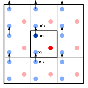
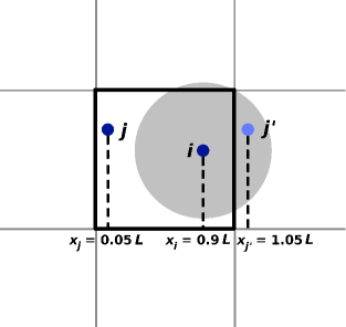
Figure 3: Schematic of PBC in two dimensions. (a) The simulation box at the center (i.e., the main system, or the primary cell) contains two particles shown in dark red and dark blue. The neighboring boxes, however, indicate the image systems composed of image particles shown in light red and light blue. As the blue particle leaves the box by moving from ${\mathrm{{\bf{X}}_{1}}}$ to ${\mathrm{{\bf{X^{\prime}}}_{1}}}$, its image simultaneously enters from the opposite side from ${\mathrm{{\bf{X^{\prime}}}_{2}}}$ to ${\mathrm{{\bf{X}}_{2}}}$, and this happens for all image cells. (b) The simulation box with size $L$ and the cutoff sphere of radius $r_{c}=L\big{/}2$ shown by the gray area. The system is composed of two particles i and j, however, i only interacts with the image of j, namely j’.

3.5.2 Purpose II

PBC are also necessary when we use short-range potentials, and are going to eliminate particles outside the cutoff radius. We know that because of PBC, particle $i$ within the primary cell interacts not only with other particles within the primary cell, but also with those within image cells. Assume the box size to be $L$ and the cutoff radius $r_{c}=L\big{/}2$. Therefore, as seen in Fig. 3, particle $i$ only interacts with the image of $j$, namely $j^{\prime}$, because

$$R_{ij}=x_{i}-x_{j}=0.9\hskip 2.84526ptL-0.05\hskip 2.84526ptL=0.85\hskip 2.84526ptL>r_{c},$$

while

$$R_{ij^{\prime}}=x_{j^{\prime}}-x_{i}=1.05\hskip 2.84526ptL-0.9\hskip 2.84526ptL=0.15\hskip 2.84526ptL<r_{c}.$$

In such a case, $R_{ij}$ must be replaced by $R_{ij^{\prime}}$. This replacement, at the programming level, corresponds with the assignment statement Rij=Rij-sign(1.,Rij), where sign is the sign function.

For the L-J potential, $r_{c}$ is usually set to $2.50\hskip 2.84526pt\sigma$. The issue associated with the cutoff radius is that $U_{LJ}$ is not differentiable at $r=r_{c}$ (Fig. 4), therefore, the force at this point cannot be calculated.

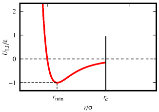
Figure 4: The L-J potential (Eq. 1) truncated at $r_{c}=2.50\hskip 1.42262pt\sigma$. That $U_{LJ}(r_{c})\neq 0$ brings about an issue in a way that the interaction force exerted on a particle suddenly vanishes at the instance it is leaving the cutoff radius.

As is seen, $U_{LJ}(r_{c})\neq 0$, and this, in turn, poses a problem in a way that the particle experiences an abrupt freedom at the instance it is leaving the cutoff sphere. The simplest way to overcome such a discontinuity is to so-called bend the potential, which is done by shifting $U_{LJ}$, namely $U_{LJ}\longrightarrow U_{LJ}-U_{LJ}(r_{c})$.

However, there still exist a couple of issues related to such a modification, which are (1) fluctuation in energy of the particle, which decreases [$E=mv^{2}/2+U_{LJ}-U_{LJ}(r_{c})$] when entering the cutoff radius and increases ($E=mv^{2}/2+U_{LJ}$) when leaving it; and (2) $U_{LJ}$ is not still differentiable at $r_{c}$. The transformation $U_{LJ}\longrightarrow U_{tot}=U_{LJ}-U_{LJ}(r_{c})-rU_{LJ}^{\prime}(r_{c})$ indeed fixes the problems. As an illustration, for the $x$ component of the force at $r_{c}$, we have

$$f_{x}(r_{c})=\frac{dU_{tot}}{dx}\Bigg{|}_{r_{c}}=\frac{dU_{tot}}{dr}\Bigg{|}_{r_{c}}\frac{dr}{dx}=\frac{dU_{LJ}}{dr}\Bigg{|}_{r_{c}}-0-U_{LJ}^{\prime}(r_{c})=0,$$

where we have used

$$\frac{dU_{tot}}{dr}=24\epsilon\bigg{(}-2\frac{\sigma^{12}}{r^{13}}+\frac{\sigma^{6}}{r^{7}}\bigg{)}-U_{LJ}^{\prime}(r_{c}),$$

and, $U_{LJ}^{\prime}=dU_{LJ}\big{/}dr$.

3.6 Thermodynamic equilibrium

From when on, is the simulation reliable for calculating statistical averages? The answer is that when the system approaches some state of thermodynamic equilibrium. Indeed, starting from random initial conditions (random positions, and velocities) definitely means the system is initially far from equilibrium, and this is while all thermodynamic properties (say temperature) are defined only at equilibrium. One way to check if the system has approached a state of thermodynamic equilibrium is to plot the time dependence of its total energy, as illustrated in Fig. 5 for an MD simulation.

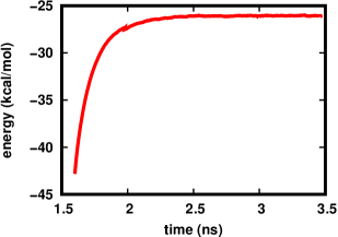
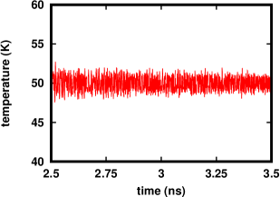
Figure 5: (a) Time dependence of the total energy of a system during an MD simulation. Over 2.5 to 3.5 ns, the energy converges meaning that the system approaches equilibrium from 2.5 ns on. In contrast, the system is entirely out of equilibrium over 1.5 to 2 ns due to a sharp variation. (b) Time dependence of the instantaneous temperature of the system discussed in (a), showing a perfect converging pattern over 2.5 to 3.5 ns of the simulation, with the equilibrium temperature of 50 K.

As is seen, the system is out of equilibrium over the first 2.5 ns because of a sharp variation and lack of convergence, in contrast to the last 1 ns with a perfect convergence, meaning that the system has reached a state of equilibrium. Time dependence of the instantaneous temperature is also very useful for checking if the system is in equilibrium. Fig. 5 illustrates such a diagram associated with the last 1 ns of Fig. 5, showing that the system is in thermodynamic equilibrium, with an average temperature of 50 K.

3.7 Degrees of freedom

In MD simulations, a $d$-dimensional system composed of $N$ particles has $(N-1)d$ degrees of freedom (DOF) instead of $Nd$. Indeed, based on the constraint that the COM velocity ($v_{cm}$) must be zero, there then exist $(N-1)$ DOF for each Cartesian component of atomic velocities, according to which there is at least one velocity being dependent on the rest:

$$v_{cm}=\sum_{i=1}^{N}v_{i}=0\hskip 8.53581pt\Longrightarrow\hskip 8.53581ptv_{1}+v_{2}+...+v_{N}=0\hskip 8.53581pt\Longrightarrow\hskip 8.53581ptv_{1}=-(v_{2}+...+v_{N}).$$

In the thermodynamic limit, $N-1\simeq N$, however, for limited numbers of particles as in all MD simulations, say $N=100$, the associated error would then be 1%, which is not negligible at all.

It is also possible to have further DOF, such as simulating water molecules with rotational and vibrational DOF, each of which gives $k_{B}T\big{/}2$ according to the equipartition theorem. One can use this theorem only in say $x$ direction to estimate the temperature of the system, without the need to know all components of the velocities. One way to test the reliability of MD simulations, in fact, is that the temperature values obtained from different DOF, or along different spatial directions, must be the same.

3.8 Velocity autocorrelation function

Using the velocity autocorrelation function [$C_{v}(\tau)$], one could have an estimation of the equilibrium time of the system. Indeed, $C_{v}(\tau)$ measures how velocity at $t+\tau$ is correlated with its value at $t$, giving therefore an estimation of the time during which the system loses its memory of previous atomic velocities. By definition,

$$C_{v}(\tau)=\frac{\langle v_{i}(t)v_{i}(t+\tau)\rangle-\langle v_{i}(t)v_{i}(t-\tau)\rangle}{\sum_{i=1}^{N}\frac{1}{t_{0}}\int_{0}^{t_{0}}v_{i}^{2}(t)dt},$$ (7)

where the denominator is equal to $(N-1)dT$ for a $d$-dimensional system of $N$ particles at the equilibrium temperature $T$. $\langle v(t)\rangle$ is always zero based on the following reasoning. If the system is large enough, after an infinite time, and within a uniform and isotropic universe, the particles would accordingly move along all directions and the average velocity is then zero. However, the simulation time is very limited, but $\langle v(t)\rangle$ is still zero because

$$\langle v(t)\rangle=\sum_{i=1}^{N}\int v_{i}(t)dt=\int\sum_{i=1}^{N}v_{i}(t)dt=\int v_{cm}dt=0.$$

As a result, the second term in the numerator of Eq. 7 vanishes, and then

$$C_{v}(\tau)=\frac{\langle v_{i}(t)v_{i}(t+\tau)\rangle}{(N-1)dT}.$$

Fig. 6 illustrates a typical $C_{v}(\tau)$ for an MD simulation.

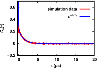
Figure 6: Velocity autocorrelation function for an MD simulation. Fitting the exponential function $e^{-\tau/\tau_{0}}$ (blue) to the obtained curve (red) gives $\tau_{0}$ as the equilibrium time of the system.

As is seen, fitting an exponential function of the form $e^{-\tau/\tau_{0}}$ to the obtained simulation data results in the value of $\tau_{0}$ as an estimation of the equilibrium time of the system.

3.9 Calculating the pressure

There are three ways to compute the pressure $P$ of the system in MD simulations, which are explained as follows.

3.9.1 Method 1

Define a plane with area $A$; compute the total number (say $N_{0}$) of particles crossing the plane during the time interval $\Delta t$; compute their associated linear momenta; and then

$$\Delta p=\sum_{i=1}^{N_{0}}2m_{i}v_{i}=F\Delta t\hskip 8.53581pt\Longrightarrow\hskip 8.53581ptF=\frac{\sum_{i=1}^{N_{0}}2m_{i}v_{i}}{\Delta t}\hskip 8.53581pt\Longrightarrow\hskip 8.53581ptP=\frac{F}{A}=\frac{\sum_{i=1}^{N_{0}}2m_{i}v_{i}}{A\Delta t},$$

where $\Delta p$ is the total momentum transferred to the plane, $F$ is the associated total force, and $m_{i}$ and $v_{i}$ are respectively the mass and velocity of particle $i$.

3.9.2 Method 2

Import one particle with the opposite velocity for each one leaving the simulation box. Therefore

$$\Delta p=F\Delta t=p_{out}-p_{in}\hskip 8.53581pt\Longrightarrow\hskip 8.53581ptF=\frac{\sum_{i}(mv_{i,\hskip 2.84526ptout}-mv_{i,\hskip 2.84526ptin})}{\Delta t}\hskip 8.53581pt\Longrightarrow\hskip 8.53581ptP=\frac{F}{A}=\frac{\sum_{i}(mv_{i,\hskip 2.84526ptout}-mv_{i,\hskip 2.84526ptin})}{A\Delta t},$$

where $p_{in}$ ($p_{out}$) is the linear momentum of the particle entering (leaving) the simulation box. It should be noted that $\Delta t$ must be large enough here to have a relatively fair approximation of the pressure.

3.9.3 Method 3

Use the kinetic theory of gases. For an ideal gas [30], $P=(N/V)k_{B}T$. However, in a more general case, if the van der Waals pair interaction is added to that ideal, $d$-dimensional system, then

$$P=\frac{N}{V}k_{B}T+\frac{1}{Vd}\Bigg{\langle}\sum_{i<j}\mathrm{\bf{F}}(\mathrm{\bf{r}}_{ij}).\mathrm{\bf{r}}_{ij}\Bigg{\rangle}=\frac{N}{V}k_{B}T-\frac{1}{Vd}\Bigg{\langle}\sum_{i<j}\frac{\partial U_{ij}}{\partial r_{ij}}r_{ij}\Bigg{\rangle},$$ (8)

which is the virial equation of state. The superiority of this method, compared to the previous, is that Eq. 8 uses all the particles to compute the pressure, also gives the instantaneous pressure of the system, without any need to wait by $\Delta t$.

The virial of the system, namely $\sum_{i}q_{i}{\dot{p}_{i}}=\sum_{i}{\mathrm{\bf{F}}}_{i}.{\mathrm{\bf{r}}}_{i}$, could have also been used to compute the pressure according to

$$P=\frac{N}{V}k_{B}T+\frac{1}{Vd}\Bigg{\langle}\sum_{i}\mathrm{\bf{F}}_{i}.\mathrm{\bf{r}}_{i}\Bigg{\rangle}.$$ (9)

However, due to PBC, for a particle leaving the box, and for its image entering from the opposite side, the two single-particle forces may be very similar, while a large jump in the single-particle position definitely takes place, leading as well to an abrupt change in the virial and then in the estimated pressure of the system. Indeed, it was this issue that led us to use double-particle forces and positions, as implemented in Eq. 8. However, one could show the equivalence between Eqs. 8 and 9 (see Appendix B).

3.10 Thermostat: Controlling the temperature

As mentioned before, the standard ensemble for MD is the microcanonical, in that the macrostate of the system is defined through the fixed numbers $N,V$, and $E$ [or, more realistically, a fixed energy range ($E,E+\Delta$)]. The basic problem is then to determine the total number $\Omega(N,V,E)$ [or, $\Omega(N,V,E;\Delta)$] of distinct, accessible microstates, from which complete thermodynamics of the system could be derived straightforwardly. For most physical systems, however, determining $\Omega$ is quite formidable if not intractable. More importantly, the concept of a fixed energy, or even a fixed energy range, for a real-world system is not satisfactory at all, based on the fact that the total energy $E$ of a system is hardly ever measured; and therefore, it is not possible to keep its value fixed in the lab.

An alternative to fixed energy is fixed temperature, which not only is measured directly in the lab using thermometers, but also is controllable and could be kept fixed by keeping the system in contact with an appropriate thermal bath. Such a so-called generalization is referred to as the canonical ensemble, in that the macrostate of the system is defined by the fixed numbers $N,V$, and $T$. This is indeed one of the most prevalent ensembles used for MD simulations.

However, keeping fixed the temperature of the system in MD simulations needs applying an extra, merely-computational trick, according to the fact that temperature, in MD simulations, becomes very quickly out of control, and takes very large values far from the defined target equilibrium temperature. This trick, at the programming level, is called thermostat, and makes the instantaneous temperature of the system to fluctuate around the target one. Although this routine works according to the equipartition theorem (Eq. 2), its presence in MD codes has no theoretical basis and is merely a matter of technique. From Eq. 2, the temperature $T$ of the system is directly correlated with atomic velocities—it is of foremost importance to mention that Eq. 2, in fact, gives the instantaneous temperature, or equivalently, the average temperature of the system at one timestep. As a result, to control the instantaneous temperature, one has to place constraint on atomic velocities. To do so, assume that the target temperature is $T_{0}$, which is not equal to instantaneous temperature $T$. Therefore, it is natural to assume that the atomic velocity $v_{i}$ times a dimensionless factor (say $\beta$) eventually leads exactly to $T_{0}$:

$$\frac{1}{Nk_{B}d}\Bigg{\langle}\sum_{i=1}^{N}m_{i}(\beta v_{i})^{2}\Bigg{\rangle}=T_{0}\hskip 5.69054pt\Longrightarrow\hskip 5.69054pt\beta^{2}T=T_{0}\hskip 5.69054pt\Longrightarrow\hskip 5.69054pt\beta=\Bigg{(}\frac{T_{0}}{T}\Bigg{)}^{1/2}.$$

As a result, the assignment statement $v_{i}=\beta v_{i}$ at the programming level, makes the average of $T$ to be very close to $T_{0}$. This kind of controlling the temperature is called rescaling. This is indeed due to rescaling the instantaneous atomic velocities that the time dependence of the thermodynamic quantities of interest (say energy, or temperature) show fluctuating patterns: every decrease after an increase in say the diagrams of Fig. 5 is accordingly the effect of multiplying the atomic velocities by $\beta$.

This method is excellent in terms of computational cost, however, it may disrupt the Maxwell–Boltzmann velocity distribution of particles. To minimize such an adverse effect, one has accordingly to apply velocity rescaling at every timestep.

4 Programming

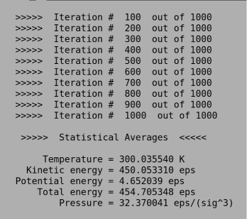
Figure 7: A typical true output of code1.py. The first ten lines are solely to inform the user that the code is being run. eps and sig respectively stand for $\epsilon$ and $\sigma$ in Eq. 1.

We have written the MD code—simulating a gas of classical, Lennard-Jones particles—in two forms in Python language (version 3.6.7). code1.py was written using top-down design, in which one starts with a large task and breaks it down to smaller pieces of program or subtasks. This is the same usual programming style used by beginners. code2.py, on the other hand, was written in a more advanced way by making use of external procedures that code each subtask as a function, each of which can be tested independently as well. It should also be noted that because the random generators applied here generate different sets of random numbers every time they are called, the outputs of any two independent runs are not exactly the same, and there is always a negligible difference. In contrast, if the difference is colossal, it then means that the issue described in Sec. 3.1 regarding very close random initial positions of one or more pairs of atoms is encountered. Therefore, it is highly recommended to run each code several times to obtain the true set of output values (see Fig. 7 for a typical true output). The notation used in these codes is also as follows.

4.1 Notation

Symbol	Description
__d__	Dimension of the simulation box (the primary cell)
NS	Total number of timesteps
N	Number of particles
dt	Time step
T_0	Target temperature
sig	$\sigma$
eps	$\epsilon$
r_ctf	Cutoff radius
u_at_ctf	Value of the potential at the cutoff
du_at_ctf	Value of the derivation of the potential at the cutoff
bs	Box size
vol	Box volume
rho	Particle density
ign	The first "ign" number of steps to be ignored for reliable statistical averaging, during which the system approaches a state of thermal equilibrium starting from an entirely out-of-equilibrium initial state due to random initial conditions
pos	Atomic positions
vel	Atomic velocities
acc	Atomic accelerations
com	Center of mass position
P_S	Sum of pressures
k_S	Sum of kinetic energies
p_S	Sum of potential energies
T_S	Sum of temperatures
f_tpz	Opens the file containing temperature, pressure, and compressiblility factor (tpz.out)
f_kpe	Opens the file containing kinetic, potential, and total energies (kpe.out)
f_xyz	Opens the file containing position coordinates (pos.xyz)
f_AVG	Opens the file containing statistical averages (means.out)
sign	Sign function
R	$r_{ij}$ scaled to box size
r	$r_{ij}$ in real units
vrl	Virial
pot	Potential energy
r_ctf	cutoff radius ($r_{c}$)
U	Lennard-Jones potential function
kin	Kinetic energy
v2	$v^{2}$
k_AVG	Average kinetic energy
p_AVG	Average potential energy
etot_AVG	Average total energy
T_i	Instantaneous temperature
B	$\beta=\sqrt{T_{0}/T}$

P	Pressure
Z	Compressibility factor, $PV\Big{/}Nk_{B}T$
step	Timestep counter

To run the codes, say code1.py, simply write in terminal (i.e., Linux command-line interface, CLI):     python3 code1.py.

4.2 MD codes in Python

4.2.1 code1.py

⬇

1#!/usr/bin/pyhon3

2import numpy as np

3from math import *

4import random

5__d__ = 3

6NS = 1000

7N = 100

8dt = 1.E-4

9T_0 = 300.

10sig = 1.

11eps = 1.

12r_ctf = 2.5*sig

13u_at_ctf = 4.*eps*((sig/r_ctf)**12 - (sig/r_ctf)**6)

14du_at_ctf = 24.*eps*(-2.*sig**12/r_ctf**13 \

15 + sig**6/r_ctf**7)

16bs = 10.*sig

17vol = bs**3

18rho = N/vol

19ign = 20

20#-------------------------------------------------

21# Initiate positions, velocities, & accelerations

22pos = np.zeros([__d__, N])

23vel = np.zeros([__d__, N])

24acc = np.zeros([__d__, N])

25for j in range (N):

26 for i in range (__d__):

27 pos[i,j] = random.uniform(0, bs)

28 vel[i,j] = random.uniform(0, 1)

29#--------------------------------------

30# Scale positions to the box size.

31pos = pos/bs

32#----------------------------

33# Translate positions to the

34# center-of-mass (com) reference frame.

35com = np.zeros ([__d__])

36for i in range(__d__):

37 for j in range(N):

38 com[i] += pos[i, j]

39 com[i] = com[i]/N

40for i in range(__d__):

41 pos[i, :] -= com[i]

42#---------------------

43P_S = 0.

44k_S = 0.

45p_S = 0.

46T_S = 0.

47f_tpz = open(’tpz.out’, ’w’)

48f_kpe = open(’kpe.out’, ’w’)

49f_xyz = open(’pos.xyz’, ’w’)

50R = np.zeros([__d__, N, N])

51r = np.zeros([__d__, N, N])

52#--------------------------

53def sign(a, b):

54 """

55 The sign function

56 """

57 if b > 0:

58 return a

59 elif b < 0:

60 return -a

61 elif b == 0:

62 return a

63#------------------------------------

64# The time evolution loop (main loop)

65for step in range(1, NS + 1):

66 #-----------------------------

67 # Periodic boundary conditions

68 pos[np.where(pos > 0.5)] -= 1

69 pos[np.where(pos < -0.5)] += 1

70 #-----------------------------

71 # Loop for computing forces

72 acc = np.zeros([__d__, N])

73 pot = np.zeros([N])

74 vrl = 0.

75 for i in range(N):

76 for j in range(i + 1, N):

77 if j != i:

78 r2 = np.zeros([N, N])

79 for k in range(__d__):

80 R[k, i, j] = pos[k, i] - pos[k, j]

81 if abs(R[k, i, j]) > 0.5:

82 R[k, i, j] -= sign(1., R[k, i, j])

83 r[k, i, j] = bs*R[k, i, j]

84 r2[i, j] += r[k, i, j]*r[k, i, j]

85 if r2[i, j] < r_ctf*r_ctf:

86 r1 = sqrt(r2[i, j])

87 ri2 = 1./r2[i, j]

88 ri6 = ri2*ri2*ri2

89 ri12 = ri6*ri6

90 sig6 = sig**6

91 sig12 = sig**12

92 u = 4.*eps*(sig12*ri12 - sig6*ri6) \

93 - u_at_ctf - r1*du_at_ctf

94 du = 24.*eps*ri2*(2.*sig12*ri12 - sig6*ri6) \

95 + du_at_ctf*sqrt(ri2)

96 pot[j] += u

97 vrl -= du*r2[i, j]

98 for k in range(__d__):

99 acc[k, i] += du*R[k, i, j]

100 acc[k, j] -= du*R[k, i, j]

101 vrl = -vrl/__d__

102 #------------------

103 # Update positions

104 pos += dt*vel + 0.5*acc*dt*dt

105 #----------------------------

106 # Compute temperature

107 kin = np.zeros([N])

108 v2 = np.zeros([N])

109 for j in range(N):

110 for i in range(__d__):

111 v2[j] += vel[i, j]*vel[i, j]*bs*bs

112 kin[j] = 0.5*v2[j]

113 k_AVG = sum(kin)/N

114 T_i = 2.*k_AVG/__d__

115 B = sqrt(T_0/T_i)

116 #--------------------------------

117 # Rescale & update the velocities

118 # according to velocity Verlet algorithm

119 vel = B*vel + 0.5*dt*acc

120 vel += 0.5*dt*acc

121 #---------------------

122 # Compute temperature

123 kin = np.zeros([N])

124 v2 = np.zeros([N])

125 for j in range(N):

126 for i in range(__d__):

127 v2[j] += vel[i, j]*vel[i, j]*bs*bs

128 kin[j] = 0.5*v2[j]

129 k_AVG = sum(kin)/N

130 T_i = 2.*k_AVG/__d__

131 B = sqrt(T_0/T_i)

132 #------------------

133 p_AVG = sum(pot)/N

134 etot_AVG = k_AVG + p_AVG

135 P = rho*T_i + vrl/vol

136 Z = P*vol/(N*T_i)

137 f_tpz.write("%e %e %e %e\n" \

138 %(step*dt, T_i, P, Z))

139 f_kpe.write("%e %e %e %e\n" \

140 %(step*dt, k_AVG, p_AVG, etot_AVG))

141 #----------------------------------

142 # Write position components

143 f_xyz.write("%d\n\n" %(step))

144 for i in range(N):

145 f_xyz.write("%e %e %e\n" %(pos[0, i]*bs, \

146 pos[1, i]*bs, pos[2, i]*bs))

147 #--------------------------------

148 if step > ign:

149 P_S += P

150 k_S += k_AVG

151 p_S += p_AVG

152 T_S += T_i

153#------------------------

154 if step%(NS*0.1) == 0: # To inform that the code is being run

155 print(">>>>> Iteration # %d out of %d" %(step, NS))

156print(’\n >>>>> Statistical Averages <<<<<\n’)

157print(’ Temperature = %f K’ %(T_S/(NS - ign)))

158print(’ Kinetic energy = %f eps’ %(k_S/(NS - ign)))

159print(’Potential energy = %f eps’ %(p_S/(NS - ign)))

160print(’ Total energy = %f eps’ %((k_S + p_S)/(NS - ign)))

161print(’ Pressure = %f eps/(sig^3)\n’ %(P_S/(NS - ign)))

4.2.2 code2.py

⬇

1#!/usr/bin/pyhon3

2import random, numpy as np

3from math import *

4#

5def PAR():

6 """

7 Simulation parameters

8 """

9 __d__ = 3

10 NS = 1000

11 N = 100

12 dt = 1.0E-4

13 T_0 = 300.

14 sig = 1.

15 eps = 1.

16 r_ctf = 2.5*sig

17 u_at_ctf = 4.*eps*((sig/r_ctf)**12 - (sig/r_ctf)**6)

18 du_at_ctf = 24.*eps*(-2.*sig**12/r_ctf**13 \

19 + sig**6/r_ctf**7)

20 bs = 10.*sig

21 vol = bs**3

22 rho = N/vol

23 ign = 20

24 return __d__, NS, N, dt, T_0, sig, \

25 eps, r_ctf, u_at_ctf, du_at_ctf, bs, vol, rho, ign

26#------------------------------------------------------

27def INIT(__d__, N, bs):

28 """

29 Initialize positions,

30 velocities,

31 and accelerations

32 """

33 pos = np.zeros([__d__, N])

34 vel = np.zeros([__d__, N])

35 acc = np.zeros([__d__, N])

36 for j in range (N):

37 for i in range (__d__):

38 pos[i, j] = random.uniform(0, bs)

39 vel[i, j] = random.normalvariate(0, 1)

40 return pos, vel, acc

41#------------------------

42def SCL(bs, pos):

43 """

44 Scale positions,

45 velocities,

46 and accelerations

47 to the box size

48 """

49 pos = pos/bs

50 return pos

51#-------------------------

52def COMREF(__d__, N, pos):

53 """

54 Translate positions

55 to the center-of-mass

56 (com) reference frame

57 """

58 com = np.zeros ([__d__])

59 for i in range(__d__):

60 for j in range(N):

61 com[i] += pos[i, j]

62 com[i] = com[i]/N

63 for i in range(__d__):

64 pos[i, :] -= com[i]

65 return pos

66#--------------

67def sign(a, b):

68 """

69 The sign function:

70 sign(a, b) returns ’a’

71 with the sign of ’b’

72 """

73 if b > 0:

74 return a

75 elif b < 0:

76 return -a

77 elif b == 0:

78 return a

79#--------------------------------------------

80def FRC(pos, N, __d__, bs, sig, eps, r_ctf, \

81 u_at_ctf, du_at_ctf):

82 """

83 Compute forces,

84 potential energy,

85 and virial

86 """

87 acc = np.zeros([__d__, N])

88 pot = np.zeros([N])

89 vrl = 0.

90 for i in range(N - 1):

91 for j in range(i + 1, N):

92 R = [pos[0, i] - pos[0, j], pos[1, i] - pos[1, j], \

93 pos[2, i] - pos[2, j]]

94 if abs(R[0]) > 0.5:

95 R[0] -= sign(1., R[0])

96 if abs(R[1]) > 0.5:

97 R[1] -= sign(1., R[1])

98 if abs(R[2]) > 0.5:

99 R[2] -= sign(1., R[2])

100 r2 = bs*bs*np.dot(R, R)

101 if r2 < r_ctf*r_ctf:

102 r1 = sqrt(r2)

103 ri2 = 1./r2

104 ri6 = ri2*ri2*ri2

105 ri12 = ri6*ri6

106 sig6 = sig*sig*sig*sig*sig*sig

107 sig12 = sig6*sig6

108 u = 4.*eps*(sig12*ri12 - sig6*ri6) \

109 - u_at_ctf - r1*du_at_ctf

110 du = 24.*eps*ri2*(2.*sig12*ri12 - sig6*ri6) \

111 + du_at_ctf/r1

112 pot[j] += u

113 vrl -= du*r2

114 for k in range(__d__):

115 acc[k, i] += du*R[k]

116 acc[k, j] -= du*R[k]

117 return acc, pot, vrl

118#--------------------------------

119def TEMP(vel, N, __d__, bs, T_0):

120 """

121 Compute instantaneous temperature

122 """

123 kin = np.zeros([N])

124 v2 = np.zeros([N])

125 for j in range(N):

126 for i in range(__d__):

127 v2[j] += vel[i, j]*vel[i, j]*bs*bs

128 kin[j] = 0.5*v2[j]

129 k_AVG = np.mean(kin)

130 T_i = 2.*k_AVG/__d__

131 B = sqrt(T_0/T_i)

132 return T_i, B, k_AVG

133#----------------------------------------------

134def EVOL(N, __d__, NS, pos, vel, acc, dt, bs, \

135 sig, eps, r_ctf, u_at_ctf, \

136 du_at_ctf, T_0, rho, vol, ign):

137 P_S = 0.

138 k_S = 0.

139 p_S = 0.

140 T_S = 0.

141 f_tpz = open(’tpz.out’, ’w’)

142 f_kpe = open(’kpe.out’, ’w’)

143 f_xyz = open(’pos.xyz’, ’w’)

144 for step in range(1, NS + 1):

145 #----------------------------

146 pos[np.where(pos > 0.5)] -= 1

147 pos[np.where(pos < -0.5)] += 1

148 #-----------------------------------

149 acc, pot, vrl = FRC(pos, N, __d__, \

150 bs, sig, eps, r_ctf, u_at_ctf, du_at_ctf)

151 vrl = -vrl/__d__

152 #---------------

153 """

154 Updating positions

155 """

156 pos += dt*vel + 0.5*acc*dt*dt

157 T_i, B, k_AVG = TEMP(vel, N, __d__, bs, T_0)

158 """

159 Update velocities

160 """

161 vel = B*vel + 0.5*dt*acc

162 acc, pot, vrl = FRC(pos, N, __d__, \

163 bs, sig, eps, r_ctf, u_at_ctf, du_at_ctf)

164 vel += 0.5*dt*acc

165 T_i, B, k_AVG = TEMP(vel, N, __d__, bs, T_0)

166 p_AVG = np.mean(pot)

167 etot_AVG = k_AVG + p_AVG

168 P = rho*T_i + vrl/vol

169 Z = P*vol/(N*T_i)

170 f_tpz.write("%d %e %e %e %e\n" \

171 %(step, step*dt, T_i, P, Z))

172 f_kpe.write("%d %e %e %e %e\n" \

173 %(step, step*dt, k_AVG, p_AVG, etot_AVG))

174 f_xyz.write("%d\n\n" %(step))

175 for i in range(N):

176 f_xyz.write("%e %e %e\n" \

177 %(pos[0, i]*bs, pos[1, i]*bs, pos[2, i]*bs))

178 if step > ign:

179 """

180 A condition for ignoring

181 the first "ign" steps

182 in order for reliable

183 statistical averaging.

184 """

185 P_S += P

186 k_S += k_AVG

187 p_S += p_AVG

188 T_S += T_i

189 if step%(NS*0.1) == 0: # To inform that the code is being run

190 print(">>>>> Iteration # %d out of %d" %(step, NS))

191 return P_S, k_S, p_S, T_S, \

192 f_tpz, f_kpe, f_xyz

193#------------------------------

194def STAVG(NS, ign, P_S, k_S, \

195 p_S, T_S, f_tpz, f_kpe, f_xyz):

196 """

197 Write statistical averages

198 """

199 f_AVG = open(’means.out’, ’w’)

200 f_AVG.write(’>>>>> Statistical Averages <<<<<\n\n’)

201 f_AVG.write(’ Temperature = %f K\n’ %(T_S/(NS - ign)))

202 f_AVG.write(’ Kinetic energy = %f eps\n’ %(k_S/(NS - ign)))

203 f_AVG.write(’Potential energy = %f eps\n’ %(p_S/(NS - ign)))

204 f_AVG.write(’ Total energy = %f eps\n’ %((k_S + p_S)/(NS - ign)))

205 f_AVG.write(’ Pressure = %f eps/(sig^3)\n’ %(P_S/(NS - ign)))

206 f_AVG.close()

207 f_tpz.close()

208 f_kpe.close()

209 f_xyz.close()

210 print(’\n>>>>> Statistical Averages <<<<<\n’)

211 print(’ Temperature = %f K’ %(T_S/(NS - ign)))

212 print(’ Kinetic energy = %f eps’ %(k_S/(NS - ign)))

213 print(’Potential energy = %f eps’ %(p_S/(NS - ign)))

214 print(’ Total energy = %f eps’ %((k_S + p_S)/(NS - ign)))

215 print(’ Pressure = %f eps/(sig^3)\n’ %(P_S/(NS - ign)))

216 return f_AVG

217#----------------------------

218__d__, NS, N, dt, T_0, sig, \

219eps, r_ctf, u_at_ctf, du_at_ctf, bs, \

220vol, rho, ign = PAR()

221#---------------------------------

222pos, vel, acc = INIT(__d__, N, bs)

223pos = SCL(bs, pos)

224pos = COMREF(__d__, N, pos)

225#--------------------------

226P_S, k_S, p_S, T_S, \

227f_tpz, f_kpe, f_xyz = EVOL(N, \

228__d__, NS, pos, vel, acc, dt, bs, sig, eps, \

229r_ctf, u_at_ctf, du_at_ctf, T_0, \

230rho, vol, ign)

231#----------------------

232f_AVG = STAVG(NS, ign, \

233P_S, k_S, p_S, T_S, \

234f_tpz, f_kpe, f_xyz)

5 Conclusions

A brief, comprehensive overview of MD simulation was provided which encompasses all the required fundamentals making this introduction self-contained. The associated computer code, simulating a gaseous system composed of classical Lennard-Jones particles was also written in Python programming language.

Appendix A Equivalence between Verlet and velocity Verlet algorithms

From Eq. 3, we have

$$x_{n+1}=2x_{n}-x_{n-1}+a_{n}h^{2}=x_{n}+\frac{1}{2}(x_{n+1}-x_{n-1})-\frac{1}{2}x_{n-1}-\frac{1}{2}x_{n+1}+x_{n}+a_{n}h^{2}$$

$$=x_{n}+v_{n}h-\frac{1}{2}a_{n}h^{2}+a_{n}h^{2}=x_{n}+v_{n}h+\frac{1}{2}a_{n}h^{2}.$$

Also, in Eq. 6, the last term is indeed the area of a trapezoid in trapezoidal integration method, which is a more better approximation compared to the rectangular analogue. This term could also be viewed as the time average of the acceleration.

Appendix B Equivalence between single- and double-particle virial terms

We have

$$\sum_{i}\mathrm{\bf{F}}_{i}.\mathrm{\bf{r}}_{i}=\sum_{i}\Bigg{(}\sum_{j}\mathrm{\bf{F}}_{ij}\Bigg{)}.\mathrm{\bf{r}}_{i}=\sum_{i}\Bigg{(}\frac{1}{2}\sum_{j}(\mathrm{\bf{F}}_{ij}-\mathrm{\bf{F}}_{ji})\Bigg{)}.\mathrm{\bf{r}}_{i}=\frac{1}{2}\sum_{i}\sum_{j}\mathrm{\bf{F}}_{ij}.\mathrm{\bf{r}}_{i}-\frac{1}{2}\sum_{i}\sum_{j}\mathrm{\bf{F}}_{ji}.\mathrm{\bf{r}}_{i}$$

$$=\frac{1}{2}\sum_{i}\sum_{j}\mathrm{\bf{F}}_{ij}.\mathrm{\bf{r}}_{i}-\frac{1}{2}\sum_{j}\sum_{i}\mathrm{\bf{F}}_{ij}.\mathrm{\bf{r}}_{j}=\frac{1}{2}\sum_{i}\sum_{j}\mathrm{\bf{F}}_{ij}.\mathrm{\bf{r}}_{i}-\frac{1}{2}\sum_{i}\sum_{j}\mathrm{\bf{F}}_{ij}.\mathrm{\bf{r}}_{j}=\frac{1}{2}\sum_{i}\sum_{j}\mathrm{\bf{F}}_{ij}.(\mathrm{\bf{r}}_{i}-\mathrm{\bf{r}}_{j})$$

$$=\sum_{i<j}\mathrm{\bf{F}}_{ij}.\mathrm{\bf{r}}_{ij}.$$

Nevertheless, PBC has a considerably less impact on $\mathrm{\bf{r}}_{ij}$ compared to the single-particle position $\mathrm{\bf{r}}_{i}$, as illustrated in Fig. 8.

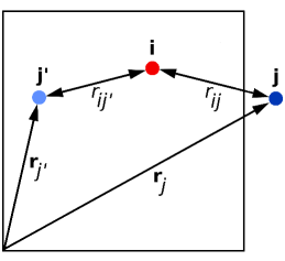
Figure 8: The simulation box (primary cell) containing the two particles i and j. As the latter leaves the box, its image, j’, simultaneously enters from the opposite side. The important point is that while single-particle positions ${\mathrm{\bf{r}}}_{j}$ and ${\mathrm{\bf{r}}}_{j^{\prime}}$ are very different compared to each other, the double-particle ones, namely $r_{ij}$ and $r_{ij^{\prime}}$, are nearly the same.

As seen in Fig. 8, there is a marked difference between single-particle positions ${\mathrm{\bf{r}}}_{j}$ and ${\mathrm{\bf{r}}}_{j^{\prime}}$, in contrast to the double-particle ones $r_{ij}$ and $r_{ij^{\prime}}$, which are nearly the same.

References

- [1] B.J. Alder, T.E. Wainwright, Studies in Molecular Dynamics. I. General Method, J. Chem. Phys. 31 (1959) 459–466.
- [2] J.M. Haile, Molecular Dynamics Simulation: Elementary Methods, John Wiley & Sons, Inc., New York, 1992.
- [3] H. Stephani, D. Kramer, M. MacCallum, C. Hoenselaers, E. Herlt, Exact Solutions of Einstein’s Field Equations, Cambridge University Press, 2003.
- [4] A. Einstein, The Foundation of the General Theory of Relativity, Ann. Phys. (Berl.) 354 (1916) 769.
- [5] D.J. Griffiths, Introduction to Quantum Mechanics, Prentice Hall, Inc., Upper Saddle River, 1995.
- [6] I.B. Cohen, Revolution in Science, Harvard University Press, Cambridge, MA, 1985.
- [7] R.K. Pathria, P.D. Beale, Statistical Mechanics, third ed., Butterworth-Heinemann, Oxford, 2011.
- [8] D.C. Rapaport, The Art of Molecular Dynamics Simulation, second ed., Cambridge University Press, Cambridge, 2004.
- [9] M. De Vivo, M. Masetti, G. Bottegoni, A. Cavalli, Role of Molecular Dynamics and Related Methods in Drug Discovery, J. Med. Chem. 59 (2016) 4035–4061.
- [10] S. Ciudad, E. Puig, T. Botzanowski, M. Meigooni, A.S. Arango, J. Do, M. Mayzel, M. Bayoumi, S. Chaignepain, G. Maglia, S. Cianferani, V. Orekhov, E. Tajkhorshid, B. Bardiaux, N. Carulla, A(1-42) tetramer and octamer structures reveal edge conductivity pores as a mechanism for membrane damage, Nat. Commun. 11 (2020) 3014.
- [11] J.E. Lennard-Jones, Cohesion, Proc. Phys. Soc. 43 (1931) 461–482.
- [12] D. Marx, J. Hutter, Ab Initio Molecular Dynamics: Basic Theory and Advanced Methods, first ed., Cambridge University Press, Cambridge, 2009.
- [13] F. Tassone, F. Mauri, R. Car, Acceleration schemes for ab initio moleculardynamics simulations and electronic-structure calculations, Phys. Rev. B 50 (1994) 10561.
- [14] J. Kohanoff, Electronic Structure Calculations for Solids and Molecules: Theory and Computational Methods, first ed., Cambridge University Press, Cambridge, 2006.
- [15] B.M. Axilrod, E. Teller, Interaction of the van der Waals type between three atoms, J. Chem. Phys. 11 (1943) 299.
- [16] A. Shekaari, M. Jafari, Non-equilibrium thermodynamic properties and internal dynamics of 32–residue beta amyloid fibrils, Physica A, 557 (2020) 124873.
- [17] M. Lutz, Learning Python, fifth ed., O’Reilly Media, 2013.
- [18] S.B. Lippman, J. Lajoie, B.E. Moo, C++ Primer, fifth ed., Addison-Wesley Professional, 2012.
- [19] S.J. Chapman, Fortran 95/2003 for Scientists and Engineers, third Ed., McGraw-Hill Education, 2007.
- [20] N. Metropolis, A.W. Rosenbluth, M.N. Rosenbluth, A.H. Teller, E. Teller, Edward, Equation of State Calculations by Fast Computing Machines, J. Chem. Phys. 21 (1953) 1087–1092.
- [21] P.M. Morse, Diatomic molecules according to the wave mechanics. II. Vibrational levels, Phys. Rev. 34 (1929) 57–64.
- [22] H. Yukawa, On the interaction of elementary particles, Proc. Phys. Math. Soc. Japan. 17 (1935) 48.
- [23] R.A. Buckingham, The Classical Equation of State of Gaseous Helium, Neon and Argon, Proc. R. Soc. A. 168 (1938) 264–283.
- [24] www.gnuplot.info.
- [25] www.gimp.org.
- [26] J.A. White, Lennard-Jones as a model for argon and test of extended renormalization group calculations, J. Chem. Phys. 111 (1999) 9352.
- [27] L. Verlet, Computer experiments on classical fluids. I. Thermodynamical properties of Lennard-Jones molecules, Phys. Rev. 159 (1967) 98.
- [28] W.C. Swope, H.C. Andersen, P.H. Berens, K.R. Wilson, A computer simulation method for the calculation of equilibrium constants for the formation of physical clusters of molecules: Application to small water clusters, J. Chem. Phys. 76 (1982) 648.
- [29] D. Beeman, Some multistep methods for use in molecular dynamics calculations, J. Comput. Phys. 20 (1976) 130–139.
- [30] A. Shekaari, M. Jafari, Effect of pairwise additivity on finite-temperature behavior of classical ideal gas, Physica A, 497 (2018) 101–108.