Transmission Line Circuit and Equation for an Electrolyte-Filled Pore of Finite Length

Abstract

I discuss the strong link between the transmission line (TL) equation and the TL circuit model for the charging of an electrolyte-filled pore of finite length. In particular, I show how Robin and Neumann boundary conditions to the TL equation, proposed by others on physical grounds, also emerge in the TL circuit subject to a stepwise potential. The pore relaxes with a timescale $\tau$, an expression for which consistently follows from the TL circuit, TL equation, and from the pore’s known impedance. An approximation to $\tau$ explains the numerically determined relaxation time of the stack-electrode model of Lian et al. [Phys. Rev. Lett. 124, 076001 (2020)].

In the early 1960s, de Levie wrote two seminal papers on electric double layer formation in porous electrodes [1, 2]. Both papers start with the transmission line (TL) circuit for an electrolyte-filled pore (Fig. 1), whose resistance $R$ and capacitance $C$ are distributed over many infinitesimally small resistors and capacitors. From this circuit, de Levie argued that $\psi(z,t)$—the electrostatic potential difference between the pore’s surface and center line at time $t$ and location $z$—follows the TL equation,

$$RC\partial_{t}\psi=\ell^{2}\partial_{z}^{2}\psi\,,$$ (1)

where, for dimensional reasons, I introduced a length scale $\ell$, which is absent in Refs. [1, 2]. Both the TL circuit and TL equation found countless applications, particularly for the interpretation for electrochemical impedance spectroscopy experiments [3, 4, 5, 6, 7]. With the ongoing interest in electrolyte-filled nanopores in general [8, 9, 10, 11, 12] and in nanoporous supercapacitors in particular [13, 14, 15], de Levie’s work is as relevant today as it was six decades ago. Yet, while Refs. [1, 2] considered Eq. 1 on a semi-infinite interval $z=[0,\infty)$, more relevant for the dc response of supercapacitors is the TL equation on a finite interval, which was studied by Biesheuvel and Bazant [13] and more recently by Gupta, Zuk, and Stone [11]. Here, I discuss the intimate relation between the TL circuit and the TL equation on a finite interval, by considering a finite-difference scheme of the latter. In particular, the Robin and Neumann boundary conditions of Refs. [13, 11], proposed there on physical grounds, also emerge in the TL circuit itself.

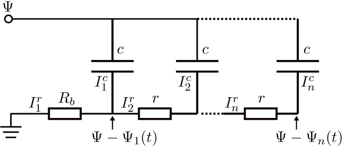
Figure 1: TL circuit with $n$ capacitors of capacitance $c$, $n-1$ resistors of resistance $r$, and one resistor of resistance $R_{b}$.

The TL circuit in Fig. 1 distributes $R$ and $C$ over $n-1$ resistors of resistance $r$ and $n$ capacitors of capacitance $c$, so that $R=r(n-1)$ and $C=cn$ . A bulk electrolyte reservoir is represented in the circuit by a resistor of resistance $R_{b}$. Now, the current from the $i$th capacitor reads $I^{c}_{i}(t)=c\dot{\Psi}_{i}(t)$ for $i=1,\ldots,n$, where $\dot{\Psi}_{i}(t)$ is the time derivative of the voltage $\Psi_{i}(t)$ across this capacitor. Kirchoff’s junction rule gives $I^{c}_{i}(t)=I^{r}_{i}(t)-I^{r}_{i+1}(t)$ for $i=1,\ldots,n-1$ and $I^{c}_{n}(t)=I^{r}_{n}(t)$, with $I^{r}_{i}(t)$ the current through the $i$th resistor; Ohm’s law states that $I^{r}_{i}(t)r=\Psi_{i-1}(t)-\Psi_{i}(t)$ for $i=2,\ldots,n$ and that $I^{r}_{1}(t)R_{b}=\Psi-\Psi_{1}(t)$, with $\Psi$ the potential of an external voltage source, suddenly applied at $t=0$. Writing $\mathbf{\Psi}(t)=\left[\Psi_{1}(t),\ldots,\Psi_{n}(t)\right]^{\intercal}$, $\mathbf{e}_{1}=\left[1,0,\ldots\right]^{\intercal}$, $\xi\equiv R/R_{b}$, and $\zeta\equiv r/R_{b}$ [hence, $\zeta=\xi/(n-1)$], I find

$$RC\dot{\mathbf{\Psi}}(t) =n\xi\Psi\mathbf{e}_{1}+n(n-1)M\mathbf{\Psi}(t)\,,$$ (2a)

$$M =\begin{bmatrix}-1-\zeta&1&&&\\ 1&-2&1&&\\ &\ddots&\ddots&\ddots&\\ &&1&-2&1\\ &&&1&-1\\ \end{bmatrix}\,,$$ (2b)

with $M\in\mathbb{R}^{n\times n}$ (cf. Ref. [14]). For initially uncharged capacitors [$\mathbf{\Psi}(0)=\mathbf{0}$], Eq. 2 is solved by

$$\frac{\mathbf{\Psi}(t)}{\Psi}=\zeta U\left[\exp{\!\left(\frac{Dn(n-1)t}{RC}\right)}-1\right]D^{-1}U^{-1}\mathbf{e}_{1}\,,$$ (3)

where $D={\rm diag}(\lambda_{1},\ldots,\lambda_{n})$ contains the eigenvalues $\lambda_{i}$ of $M=UDU^{-1}$, which are all negative.

Consider now a cylindrical pore of length $\ell$ and radius $a$ with the same resistance $R$ and capacitance $C$ as the TL circuit above, subject to the same instantaneous potential $\Psi$. The pore is closed at $z=\ell$ and in contact with a bulk reservoir of resistance $R_{b}$ at $z=0$. I study $\psi(z,t)$ in this pore through the TL equation (1) subject to Robin and Neumann boundary conditions,

$$\psi(z,0) =0\,, z\in[0,\ell]\,,$$ (4a)

$$\ell\partial_{z}\psi(0,t) =\xi[\psi(0,t)-\Psi], \partial_{z}\psi(\ell,t)=0\,.$$ (4b)

Reference [13] proposed a similar Robin condition at $z=0$ on the basis of $\psi(z)$ being linear in the reservoir ($z<0$); Ref. [11] refined the same argument for a pore with overlapping electric double layers, that is, when the Debye length is comparable to the pore’s radius $\lambda_{D}\approx a$. For that case, $\psi(z,t)$ should not reach $\Psi$ at late times, and the TL circuit must be adopted accordingly [11].

The solution to Eqs. 1 and 4 reads [17]

$$\frac{\psi(z,t)}{\Psi} =1-\sum_{j\geq 1}\frac{4\sin\beta_{j}\cos\left[\beta_{j}\left(1-z/\ell\right)\right]}{2\beta_{j}+\sin 2\beta_{j}}\exp{\!\left[-\frac{\beta_{j}^{2}t}{RC}\right]}\,,$$ (5a)

where $$\beta_{j} j=1,2,\ldots$$ with are the solutions of the transcendental equation

$$\beta_{j}\tan\beta_{j}=\xi\,.$$ (5b)

For comparison, I also mention the solution to Eq. 1 on a semi-infinite slab $z\in[0,\infty)$ subject to the same Robin condition at $z=0$ [18],

$$\frac{\psi(z,t)}{\Psi} =-\exp\left[\xi\frac{z}{\ell}+\xi^{2}\frac{t}{RC}\right]\mathrm{erfc}\left[\sqrt{\frac{z^{2}}{\ell^{2}}\frac{RC}{4t}}+\xi\sqrt{\frac{t}{RC}}\right]$$

$$\quad+\mathrm{erfc}\sqrt{\frac{z^{2}}{\ell^{2}}\frac{RC}{4t}}\,.$$ (6)

Note that $R_{b}$ entered the TL equation through the Robin condition Eq. 4b. For $\xi=R/R_{b}\to\infty$, this Robin condition simplifies to de Levie’s Dirichlet condition [1]. In this limit, Eq. 5b simplifies to $\cos\beta_{j}=0$—solved by $\beta_{j}=(j-1/2)\pi$—and $\psi(z,t)$ simplifies accordingly. Meanwhile, only the last term of Transmission Line Circuit and Equation for an Electrolyte-Filled Pore of Finite Length remains for $\xi\to\infty$ and $\psi(z,t)$ reduces to Eq. 9 of Ref. [1].

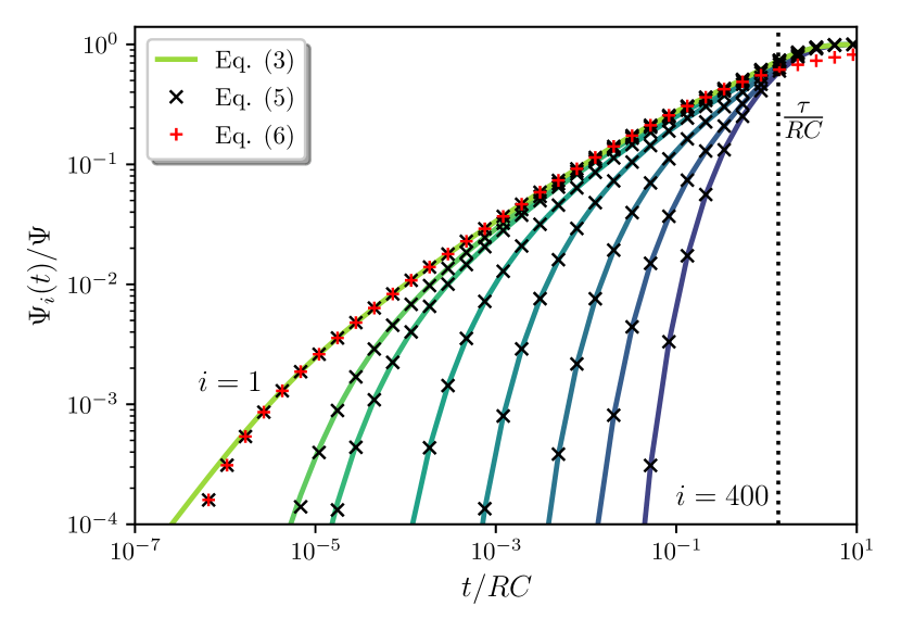
Figure 2: TL-circuit potential drops $\Psi_{i}(t)$ [Eq. 3, lines] and TL-equation solutions $\psi\bm{(}z/\ell=(i-1/2)/n,t\bm{)}$ [Eq. 5, crosses] and $\psi\bm{(}z=\ell/(2n),t\bm{)}$ [Transmission Line Circuit and Equation for an Electrolyte-Filled Pore of Finite Length, pluses], all divided by $\Psi$, for $i=(1,3,5,15,40,100,200,400)$, $n=400$, and $\xi=R/R_{b}=1$. The sum in Eq. 5a is truncated after ${\rm max}(j)=1000$. The dotted line indicates the late-time relaxation time $\tau=RC/\beta_{1}^{2}$.

Figure 2 shows $\Psi_{i}$ [Eq. 3, lines] and $\psi\bm{(}z=(i-1/2)\ell/n,t\bm{)}$ [Eq. 5, crosses] for $R_{b}=R$, $n=400$, and $i=(1,3,5,15,40,100,200,400)$. As $\Psi_{i}$ describes the potential drop between the pore’s surface and centerline along the pore from $z=(i-1)\ell/n$ to $z=i\ell/n$, I evaluate $\psi$ at the center of this interval. Figure 2 shows that predictions from Eqs. 3 and 5 agree well, except for $i=1$ and $t/RC<10^{-6}$. For comparison, Fig. 2 also shows $\psi\bm{(}z=\ell/(2n),t\bm{)}$ from Transmission Line Circuit and Equation for an Electrolyte-Filled Pore of Finite Length (pluses). Predictions from Eqs. 5 and Transmission Line Circuit and Equation for an Electrolyte-Filled Pore of Finite Length coincide up to $t\approx RC$, when the potential perturbations reach $z=\ell$ and, hence, the Neumann condition in Eq. 4b becomes important.

To better understand why Eqs. 3 and 5 agree so well, I turn to a finite-difference description of Eqs. 1 and 4. Following Ref. [19], I discretise $z$, but not $t$. Partitioning $[0,\ell]$ into $m-1$ intervals of width $h=\ell/(m-1)$ yields a uniform grid of $m$ grid points, at $z_{k}=kh$ with $k\in\{0,\ldots,m-1\}$. On these grid points, the continuous electrostatic potential is approximately $\psi_{k}=\psi(z_{k})$. A central difference approximation now gives $\partial_{z}^{2}\psi(z_{k})\simeq(\psi_{k-1}-2\psi_{k}+\psi_{k+1})/h^{2}$. To implement the Robin boundary condition at $z=0$, I introduce a ghost grid point at $z=-h$ and corresponding $\psi_{-1}$. Now, approximating the $z$ derivative through a backward difference $\partial_{z}\psi(0)\simeq(\psi_{0}-\psi_{-1})/h$, the Robin boundary condition yields $\psi_{-1}=\psi_{0}+\xi(\Psi-\psi_{0})/(m-1)$. Similar reasoning and a forward difference yields for the Neumann condition that $\psi_{m}=\psi_{m-1}$ [19]. After grouping the above expressions and writing $\bm{\psi}(t)=\left[\psi_{1}(t),\ldots,\psi_{m-1}(t)\right]^{\intercal}$, Eqs. 1 and 4 are approximated by

$$RC\dot{\bm{\psi}}(t)=(m-1)\xi\Psi\mathbf{e}_{1}+(m-1)^{2}M\bm{\psi}(t)\,,$$ (7)

with $M\in\mathbb{R}^{m\times m}$ as in Eq. 2b. Setting $m=n$, Eqs. 7 and 2 are very similar: the prefactors on their right-hand sides contain differences that are of subleading order in $n$. Indeed, replotting Fig. 2 for smaller $n$, I observed that differences between Eqs. 3 and 5 became larger, while for $n>500$, both methods were practically indistinguishable (not shown). Note, first, that the differences between Eqs. 3 and 5 are unrelated to the truncation of Eq. 5 at finite $j$: my numerical observation that this sum was converged is reinforced by the overlap of Eqs. 5 and Transmission Line Circuit and Equation for an Electrolyte-Filled Pore of Finite Length at early times. Second, note that differences between Eqs. 7 and 2 of subleading order in $n$ could not be circumvented altogether, for instance, by changing the TL circuit or the above finite-difference scheme: the order of $M$ in Eq. 2a is equal to the number of capacitors in the circuit, which also sets the factor $n$ in $n(n-1)M$. Conversely, in Eq. 7, the order of $M$ is given by the number of grid points, while the prefactor of $M$ is set by the number of intervals, which is always one smaller. Lastly, differences between Eqs. 7 and 2 being of subleading order in $n$ means that those equations are equal in the limit $n\to\infty$. Thus, different from the physical arguments of Refs. [11, 13], both the Robin and the Neumann boundary condition in Eq. 4b also emerge naturally in the TL circuit and Eq. 2, which governs its relaxation.

Important for applications of porous electrodes, Fig. 2 suggests that $\psi(z,t)$ relaxes with a single late-time relaxation time, denoted $\tau$, throughout the pore. This observation stands in contrast to de Levie’s solution to the TL equation on a semi-infinite interval—the last term of Transmission Line Circuit and Equation for an Electrolyte-Filled Pore of Finite Length—which relaxes with a position-dependent relaxation time $(z/\ell)^{2}RC/4$ [1]. From Eq. 5 it follows that $\tau=RC/\beta_{1}^{2}$, with $\beta_{1}$ the smallest solution to Eq. 5b. For example, $\xi=1$ yields $\tau/RC\approx 1.35$, shown with a dotted line in Fig. 2. Conversely, by the above-mentioned simplification of Eq. 5b, $\xi\to\infty$ yields $\tau/RC=4/\pi^{2}$ [8, 12].

The same relaxation behavior follows from the TL circuit: as all eigenvalues $\lambda_{i}$ of $M$ are negative, it follows from Eq. 3 that $\mathbf{\Psi}(t)$ relaxes at late times with the timescale

$$\tau=-\frac{RC}{n(n-1)\lambda_{+}}\,,$$ (8)

with $\lambda_{+}=\max\{\lambda_{1},\ldots,\lambda_{n}\}$ the least negative eigenvalue of $M$. For matrices of $M$’s form, the different $\lambda_{i}$ satisfy

$$U_{n}\left(\frac{\lambda_{i}}{2}+1\right)-U_{n-1}\left(\frac{\lambda_{i}}{2}+1\right)=$$

$$\quad\quad\left(1-\zeta\right)\left[U_{n-1}\left(\frac{\lambda_{i}}{2}+1\right)-U_{n-2}\left(\frac{\lambda_{i}}{2}+1\right)\right]\,,$$ (9)

where $U_{n}$ are $n$th degree Chebyshev polynomials of the second kind . With $U_{n}\left(\cos\vartheta\right)=\sin\bm{(}\left(n+1\right)\vartheta\bm{)}/\sin\vartheta$, inserting $\lambda_{i}=2\left[\cos(\vartheta_{i})-1\right]$ into Transmission Line Circuit and Equation for an Electrolyte-Filled Pore of Finite Length yields,

$$\frac{\sin\bm{(}\left(n+1\right)\vartheta_{i}\bm{)}-\sin\left(n\vartheta_{i}\right)}{1-\zeta}=\sin\left(n\vartheta_{i}\right)-\sin\bm{(}\left(n-1\right)\vartheta_{i}\bm{)}\,.$$ (10)

Using $\sin(\alpha\pm\beta)=\sin(\alpha)\cos(\beta)\pm\sin(\beta)\cos(\alpha)$ and dividing both sides of Eq. 10 by $\sin(n\vartheta_{i})\sin\vartheta_{i}$ yields

$$\frac{2-\zeta}{\zeta}\tan\left(n\vartheta_{i}\right)=\frac{\sin\vartheta_{i}}{1-\cos\vartheta_{i}}\,.$$ (11)

The smallest solution $\vartheta_{-}$ to Eq. 11, required to find $\lambda_{+}=2\left[\cos(\vartheta_{-})-1\right]$, lies in the interval $\vartheta_{-}\in[0,\pi/(2n)]$. Thus, for $n\gg 1$, one has $\vartheta_{-}\ll 1$ and thus $\lambda_{+}=-\vartheta_{-}^{2}+O(\vartheta_{-}^{4})$. Now, for $n\gg 1$ and provided that $\xi/n\ll 1$, Eq. 11 reduces to

$$n\vartheta_{-}\tan\left(n\vartheta_{-}\right)=\xi+O\left(n^{-1}\right)\,.$$ (12)

Hence, for $n\gg 1$, the late-time relaxation times of the TL circuit and the TL equation are governed by the same transcendental equation [Eqs. 5b and 12].

A Padé approximation of order $[1/2]$ of the $\tan(n\vartheta_{-})$ term in Eq. 12 yields the approximate solution [22]

$$n\vartheta_{-}\approx\sqrt{\frac{3\xi}{3+\xi}}\,.$$ (13)

From Eq. 8 now follows the late-time response of the TL circuit as

$$\tau\approx\frac{1}{3}RC+R_{b}C\,.$$ (14)

This expression is inaccurate for small $R_{b}$: in the limit $\xi\to\infty$, the TL circuit expression Eq. 12 simplifies to $\cos\left(n\vartheta_{-}\right)=0$. As anticipated, its solution $\vartheta_{-}=\pi/(2n)$ yields $\tau=4RC/\pi^{2}$, suggesting that the factor $1/3$ in Eq. 14 should be replaced by $4/\pi^{2}\approx 0.41$,

$$\tau\approx\frac{4}{\pi^{2}}RC+R_{b}C\,.$$ (15)

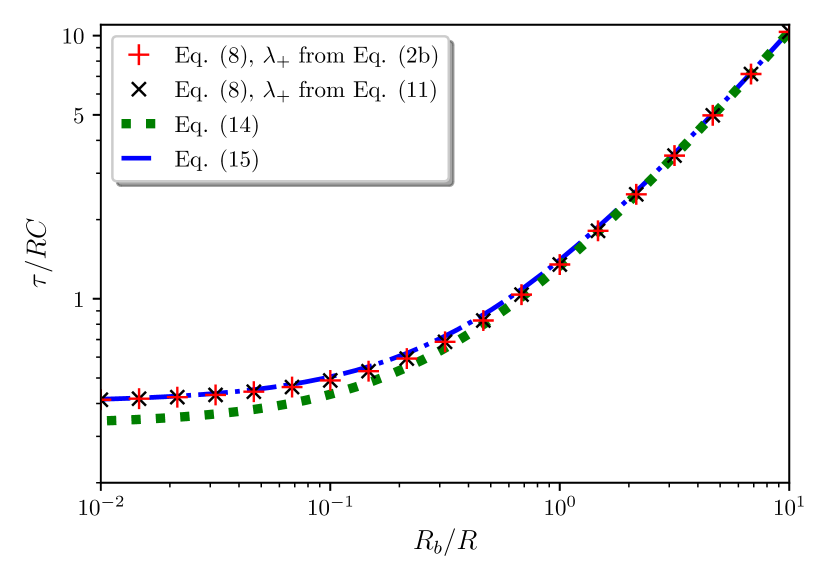
Figure 3: Late-time relaxation time $\tau$ [Eq. 8] for $n=100$, with $\lambda_{+}$ determined numerically from $M$ (pluses) and Eq. 11 (crosses). Also shown are the approximate solutions Eq. 14 (dotted line) and Eq. 15 (dash-dotted line).

Figure 3 shows $\tau$ [Eq. 8] with $\lambda_{+}$ determined from $M$ directly (red pluses) and from Eq. 11 (black crosses) as well as the approximations Eq. 14 (dotted line) and Eq. 15 (dash-dotted line). Since crosses and pluses overlap, Eq. 11 successfully captures $\lambda_{+}$. As expected, Eq. 14 accurately approximates $\tau$ for $R_{b}/R\gg 1$ but not for $R_{b}/R\lessapprox 1$. Conversely, Eq. 15 is in excellent agreement with Eq. 8 at both $R_{b}/R\ll 1$ and $R_{b}/R\gg 1$ but slightly less so around $R_{b}/R\approx 1$.

There is yet another route to the timescale $\tau$ with which a finite-length pore relaxes in response to a stepwise potential: through its known impedance $Z(\mathrm{i}\hskip 0.56905pt\omega)=\sqrt{R/(\mathrm{i}\hskip 0.56905pt\omega C)}\coth\sqrt{\mathrm{i}\hskip 0.56905pt\omega RC}$ [3]. Here, $\mathrm{i}=\sqrt{-1}$ and $\omega$ is the angular frequency of a sinusoidal potential applied to the pore. At low frequencies $\hat{Z}(s\approx 0)\approx\hat{Z}_{l}(s)=R/3+1/(Cs)$, where the complex frequency $s$ appears instead of $\mathrm{i}\hskip 0.56905pt\omega$ [4, 5]. The same $\hat{Z}_{l}(s)$ applies to a series connection of a resistor of resistance $R/3$ and a capacitor of capacitance $C$. To account for the bulk with which the pore is in contact, I add a resistor of resistance $R_{b}$ in series with these two elements. Subjecting this circuit to a step potential $V(t)=V_{0}\Theta(t)$, with $\Theta(t)$ the Heaviside function, drives a current $I(t)=\mathcal{L}^{-1}\{\hat{V}(s)/[\hat{Z}_{l}(s)+R_{b}]\}\propto\exp[-t/\tau]$, with $\mathcal{L}^{-1}$ the inverse Laplace transform, $\hat{V}(s)=\mathcal{L}\{V(t)\}=V_{0}/s$, and $\tau$ precisely as in Eq. 14. Yet, inverse Laplace transformations of approximate expressions yield wrong relaxation times if the original function has different poles than its approximation [23]. Such is the case for $1/\hat{Z}_{l}(s)$. The exact current $I(t)=\mathcal{L}^{-1}\{\hat{V}(s)/[\hat{Z}(s)+R_{b}]\}$ relaxes at late times with $\tau=-1/s^{*}$, with $s^{*}$ the first solution to $\sqrt{R/(sC)}\coth\sqrt{sRC}+R_{b}=0$ on the negative $s$ axis. Substituting $sRC=-\beta_{j}^{2}$, we recover Eq. 5b; hence, $I(t)$ relaxes precisely as $\psi(z,t)$ in Eq. 5a.

While several papers included a bulk resistance in the TL circuit [2, 13, 11], the influence of $R_{b}$ on the relaxation of the TL circuit is not generally recognized, Ref. [24] being a notable exception. The often-used TL timescale $\lambda_{D}\ell^{2}/(Da)$ [13, 8, 9, 11], with $D$ the ionic diffusivity, does not account for $R_{b}C$, nor for $RC$’s prefactors in Eqs. 14 and 15. Hence, depending on the geometry of interest, particularly on the distance of the pore to a counter electrode, a pore’s relaxation time can deviate significantly from $\lambda_{D}\ell^{2}/(Da)$. Still, in electrodes with ultranarrow pores—much beyond the validity of the TL equation—attenuation of the in-pore diffusivity probably yields $R\gg R_{b}$, making pore entrance the rate-limiting step of electrode charging [15].

As a corollary, I show how Eq. 14 sheds light on the recently proposed stack-electrode model for supercapacitor charging [14]. In this model, a porous electrode of thickness $H$ was represented by a stack of $n$ flat, metallic yet permeable sheets of area $A$, with a constant spacing $h$, so that $r=h\lambda_{D}^{2}/(\varepsilon DA)$ and $c=2\varepsilon A/\lambda_{D}$. Two such electrodes were in contact with a bulk of length $2L$; hence, $R_{b}/R=L/H$. Equation 14 now yields $\tau=(2+2H/3L)n\lambda_{D}L/D$, which, for large $n$, is in reasonable agreement with the fitted timescale $\tau_{n}=[\left(2+0.75H/L\right)n-1-0.91H/L]\lambda_{D}L/D$ of Ref. [14]. While both $\tau_{n}$ and $\tau$ from Eq. 14 are based on approximations, differences between them must also stem from the different $n$th sheet in the stack-electrode model, which had half the capacitance of the other sheets. As $\tau_{n}$ captured the short timescale of the biexponential current decay in the experiments of Ref. [25], $\tau$ as calculated here accurately describes the same timescale as well . The stack-electrode model also captured the second, larger timescale of the transient current measured in Ref. [25] and ascribed it to the $0.1\text{\,}\mathrm{V}$ applied there—large, compared to the thermal voltage of $24\text{\,}\mathrm{mV}$. Such potentials fall outside the region of validity of the TL equation [13].

Concluding, I have exposed the intimate relation between the TL circuit model for a pore in contact with an electrolyte reservoir and the TL equation subject to Robin and Neumann boundary conditions. The pore relaxes with a $R_{b}/R$-dependent relaxation time that explains one of the two dominant relaxation timescales of Refs. [14, 25].

I thank Carlos da Fonseca and Cheng Lian for inspiring discussions, Christian Pedersen and Stephane Poulain for useful comments on this work, and an anonymous referee for pointing out $\hat{Z}_{l}(s)=R/3+1/(Cs)$ to me. The research leading to these results has received funding from the European Union’s Horizon 2020 research and innovation programme under the Marie Skłodowska-Curie grant agreement No 801133.

References

- de Levie [1963] R. de Levie, Electrochim. Acta 8, 751 (1963).
- de Levie [1964] R. de Levie, Electrochim. Acta 9, 1231 (1964).
- de Levie [1967] R. de Levie, in Advances in Electrochemistry and Electrochemical Engineering (Wiley-Interscience, New York, 1967), Vol. 6, pp. 329–397, Eq. (98).
- Bisquert [2002] J. Bisquert, J. Phys. Chem. B 106, 325 (2002).
- Barsoukov and Macdonald [2005] E. Barsoukov and J. R. Macdonald, Impedance Spectroscopy Theory, Experiment, and Applications (John Wiley & Sons, Hoboken, 2018).
- Newman and Thomas-Alyea [2012] J. Newman and K. E. Thomas-Alyea, Electrochemical Systems (John Wiley & Sons, New York, 2004).
- Conway [2013] B. E. Conway, Electrochemical Supercapacitors: Scientific Fundamentals and Technological Applications (Academic/Plenum Publishers, New York, 1999).
- Mirzadeh et al. [2014] M. Mirzadeh, F. Gibou, and T. M. Squires, Phys. Rev. Lett. 113, 097701 (2014).
- Tivony et al. [2018] R. Tivony, S. Safran, P. Pincus, G. Silbert, and J. Klein, Nat. Commun. 9, 1 (2018).
- Perez-Martinez and Perkin [2019] C. S. Perez-Martinez and S. Perkin, Soft Matter 15, 4255 (2019).
- Gupta et al. [2020] A. Gupta, P. J. Zuk, and H. A. Stone, Phys. Rev. Lett. 125, 076001 (2020).
- Timur et al. [2020] A. Timur, K. Sinkov, and I. Akhatov, arXiv:2011.04575v2.
- Biesheuvel and Bazant [2010] P. M. Biesheuvel and M. Z. Bazant, Phys. Rev. E 81, 031502 (2010).
- Lian et al. [2020] C. Lian, M. Janssen, H. Liu, and R. van Roij, Phys. Rev. Lett. 124, 076001 (2020), Eqs. (4) and (S15).
- Breitsprecher et al. [2020] K. Breitsprecher, M. Janssen, P. Srimuk, B. L. Mehdi, V. Presser, C. Holm, and S. Kondrat, Nat. Commun. 11, 6085 (2020).
- Note [1] The circuit in Fig. 1 does not account for Faradaic reactions on the electrode surface, typically modeled through a Faradaic impedance parallel to the capacitors [7].
- Beck et al. [1992] J. V. Beck, K. D. Cole, A. Haji-Sheikh, and B. Litkouhl, Heat Conduction using Green’s Functions, 2nd ed. (Taylor & Francis, London, 2011), p. 208-211.
- Carslaw and Jaeger [1959] H. S. Carslaw and J. C. Jaeger, Conduction of heat in solids, 2nd ed. (Clarendon Press, Oxford, 1959), p. 72.
- Strang and MacNamara [2014] G. Strang and S. MacNamara, SIAM Rev. 56, 525 (2014).
- Note [2] in Eq. (1.1) of Ref. [21] equals [Eq. 2b]. Notably, Eq. (2.1) of Ref. [21] yields not the spectrum of , as stated there, but of .
- da Fonseca [2007] C. da Fonseca, J. Comput. Appl. Math. 200, 283 (2007).
- Wu et al. [2018] B. Wu, W. Liu, Z. Yang, and X. Chen, J. Phys. Commun. 2, 055009 (2018), Eq. (9).
- Janssen and Bier [2018] M. Janssen and M. Bier, Phys. Rev. E 97, 052616 (2018).
- Kroupa et al. [2016] M. Kroupa, G. J. Offer, and J. Kosek, J. Electrochem. Soc. 163, A2475 (2016).
- Janssen et al. [2017] M. Janssen, E. Griffioen, P. M. Biesheuvel, R. van Roij, and B. Erné, Phys. Rev. Lett. 119, 166002 (2017).
- Note [3] A stagnant diffusion layer is sometimes introduced in lieu of the bulk reservoir length [13, 11]. This choice would yield in worse agreement with Ref. [25].