Dimension reduction of open-high-low-close data in candlestick chart based on pseudo-PCA

Abstract

The (open-high-low-close) OHLC data is the most common data form in the field of finance and the investigate object of various technical analysis. With increasing features of OHLC data being collected, the issue of extracting their useful information in a comprehensible way for visualization and easy interpretation must be resolved. The inherent constraints of OHLC data also pose a challenge for this issue. This paper proposes a novel approach to characterize the features of OHLC data in a dataset and then performs dimension reduction, which integrates the feature information extraction method and principal component analysis. We refer to it as the pseudo-PCA method. Specifically, we first propose a new way to represent the OHLC data, which will free the inherent constraints and provide convenience for further analysis. Moreover, there is a one-to-one match between the original OHLC data and its feature-based representations, which means that the analysis of the feature-based data can be reversed to the original OHLC data. Next, we develop the pseudo-PCA procedure for OHLC data, which can effectively identify important information and perform dimension reduction. Finally, the effectiveness and interpretability of the proposed method are investigated through finite simulations and the spot data of China’s agricultural product market.

Key Words: OHLC data; pseudo-PCA; dimension reduction; feature information extraction

1 Introduction

As one of the most classic technical analysis tools, the candlestick chart is used to document the prices of almost all financial products, including spots, stocks, futures, options, etc (Romeo et al., 2015; Chmielewski et al., 2015). Investors can judge the long and short trading conditions and roughly predict future price trends by analyzing candlestick chart (Tsai and Quan, 2014).

Intuitively, Figure.1 shows a daily candlestick chart, which not only records the open price, high price, low price, and close price of certain object on that day, but also reflects the difference between any two prices. According to American convention, a green real body refers to a bull market (the close price $\textgreater$ the open price, see Figure.1(a)), while a red real body refers to a bear market (the open price $\textgreater$ the close price, see Figure.1(b)), respectively.

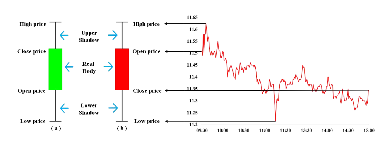
Fig. 1: An example of daily candlestick chart

Mathematically, the essence of the candlestick chart is a $4$-dimensional vector, consisting of the open price, high price, low price, and close price, which are collectively called the OHLC data (Kazemilari and Djauhari, 2015). However, unlike ordinary $4$-dimensional vectors, the OHLC data have some important inherent constraints. Specifically,

Definition 1.

A $4$-dimensional vector $\bm{x}=(x^{(o)},x^{(h)},x^{(l)},x^{(c)})^{\prime}$ is considered the OHLC data if $\bm{x}$ satisfies the following three constraints:

(1) $x^{(l)}>0$;

(2) $x^{(l)}<x^{(h)}$;

(3) $x^{(o)},x^{(c)}\in[x^{(l)},x^{(h)}]$.

where $x^{(o)},x^{(h)},x^{(l)}$ and $x^{(c)}$ represent the open price, high price, low price, and close price of the subject during a certain time period (which can vary from seconds to months), respectively.

The OHLC data $\bm{x}$ in Definition.1 can be defined as a generalized interval-valued data from the perspective of symbolic data analysis (Diday, 1988). Namely, the OHLC data takes $x^{(h)}$ and $x^{(l)}$ as the upper and lower boundaries of the interval, while $x^{(o)}$ and $x^{(c)}$ lie within the interval. Compared to the interval-valued data, the OHLC data contains more information, resulting in more complicated properties than interval-valued data. The common methods for interval-valued data, such as the Max $\&$ Min method (Arroyo et al., 2011) and Center $\&$ Range (Brito and Duarte Silva, 2012; Giordani, 2015) method are mimicked by various works on the OHLC data. For example, Yang et al. (2012), Xiong et al. (2017), and Sun et al. (2018) have investigated the OHLC data via the above methods used for interval-valued data without incorporating information on the open price and close price.

Owing to the ignorance of the open price and close price, these two widely-used methods cannot completely use the OHLC data information, yielding possible inefficient results. As indicated by Cheung (2007), the open price and close price have an explanatory power for the fluctuation of the OHLC data and should be carefully incorporated into statistical modeling.

Through decades of development, scholars have completed multi-angle studies on the candlestick chart and its data (i.e., OHLC data). Initially, scholars are committed to performing pattern recognition on the candlestick chart (Kamijo and Tanigawa, 1990; Juang and Katagiri, 1992; Lo et al., 2000; Cervelló-Royo et al., 2015), giving priority to finding a candlestick chart pattern that could obtain stable profits. At the same time, traditional statistical methods such as the clustering analysis (Harris, 1991; Brown et al., 2002; Tao et al., 2017) and discriminant analysis (Hopkins, 1996; Leung et al., 2000; Cohen et al., 2019) have also been gradually applied to the study of the candlestick chart. In addition, other popular researches include predicting the future changes of OHLC data, such as econometric forecasting models (Fiess and MacDonald, 2002; Pai and Lin, 2005; De Nard et al., 2020) and machine learning models (Cao and Tay, 2003; Liu and Wang, 2012; Mann and Gorse, 2017; Mallqui and Fernandes, 2019).

With technological advances in many scientific areas, a considerable amount of OHLC data is available. It is crucial to develop a dimension reduction technique to extract the informative features contained in the multivariate OHLC data. Among the dimension reduction methods, the principal component analysis (PCA) has always been a key technique to extract the comprehensive features using the linear combination of the original variables, which are called principal components (PCs). These PCs represent the major mode of data variation and are the characterizing features of typical variables in a dataset (Wang et al., 2015; M’ng and Mehralizadeh, 2016). Furthermore, the scores on PCs have been used for visualization to help researchers better understand the correlation between the original variables (Jolliffe, 2002).

Nonetheless, the aforementioned PCA method is not applicable when handling dimension reduction for the OHLC data due to its inherent constraints, which poses new challenges. For example, imposing the classical PCA on the OHLC dataset will destroy its structure, rendering the corresponding PCs meaningless. Furthermore, as a special type of data, the OHLC data is characterized as a $4$-dimensional vector data with constraints defined in Definition.1 as a whole, which is completely different from the classical scalar data or the vector data in the Euclidean space. All of these concerns are motivations to propose a new approach.

As a reminder, the OHLC data can be used as generalized interval-valued data. Fortunately, various PCA techniques have been extended from classical scalar data to the interval-valued data, such as the vertices principal component analysis (VPCA; Cazes et al. (1997)) , centers principal component analysis (CPCA; Chouakria et al. (2000)), symbolic object principal component analysis (SPCA; Lauro and Palumbo (2000)), midpoints radii principal component analysis (MRPCA; Palumbo and Lauro (2003)), interval principal component analysis (IPCA; Gioia and Lauro (2006)), and complete-information-based principal component analysis (CIPCA; Wang et al. (2012)). After revisiting the aforementioned PCA methods for interval-valued data, we find that the key point is to extract feature-based representation of interval-valued data, such as vertices, midpoint, radii, etc. Nonetheless, these existing approaches are only designed for interval-valued data, and they could not be directly applied to the OHLC data. Apart from the two boundaries contained in the interval-valued data, the OHLC data includes more information and constraints. Consequently, this requires more feature-based representations.

Therefore, this paper aims to explore dimension reduction for the OHLC data based on the PCA method with the idea of feature-based representations, constructing a novel approach to characterize features of OHLC data. First, we propose a new way to represent the OHLC data, which can eliminate the inherent constraints and make further analysis easier. Furthermore, there is a one-to-one match between the original OHLC data and its feature-based representations, which allows the analysis of the feature-based representations to be reversed to the original data. Next, we develop the pseudo-PCA procedure for OHLC data, which can effectively identify important information and perform dimension reduction. Finally, the effectiveness and interpretability of the proposed method are investigated through finite simulations and the spot data of China’s agricultural product market.

This paper has two main contributions. First, a novel feature-based representation method is proposed for the OHLC data, which provides a new perspective and facilitates further statistical analysis of the OHLC data. Second, we introduce a pseudo-PCA procedure to achieve dimension reduction for multivariate OHLC data, which enhances existing literature on PCA methods.

The rest of the paper is organized as follows: Section 2 presents the feature extraction method for the OHLC data and related algebraic space of the feature-based representations. In Section 3, we describe the proposed pseudo-PCA procedure. Then we examine the effectiveness, robustness and interpretability of the pseudo-PCA by simulations in Section.4 and empirical experiment in Section 5. Finally, we conclude with a brief summary and insights, as well as several possible further research topics in Section 6.

2 Feature-based representations and its algebraic space

2.1 Feature-based representations of OHLC data

Inspired by the feature extraction method for interval-valued data, we propose a novel feature-based representation approach for the OHLC data in Definition.2. This satisfies the following merits: First, each component of feature-based representations has a unique and meaningful interpretation of the OHLC data. Second, it eliminates the inherent constraints and provides convenience for further analysis. Third, there is a one-to-one match between the original OHLC data and its feature-based representations, which allows the analysis of the feature-based representations to be reversed to the original data.

Definition 2.

(Feature-based representations of OHLC data). For the OHLC data $\bm{x}=(x^{(o)},x^{(h)},x^{(l)},x^{(c)})^{\prime}$, assume that $x^{(o)},x^{(h)},x^{(l)}$, and $x^{(c)}$ are not equal to each other $(\text{except for}\;x^{(o)}\equiv x^{(c)})$, then the feature-based representation of $\bm{x}$ is formulated as $\bm{y}=(y^{(1)},y^{(2)},y^{(3)},y^{(4)})^{\prime}$, where

$$\left\{\begin{array}[]{l}y^{(1)}=\ln x^{(l)}\\ y^{(2)}=\ln(x^{(h)}-x^{(l)})\\ y^{(3)}=\ln\Big{(}\frac{\lambda^{(o)}}{1-\lambda^{(o)}}\Big{)}\\ y^{(4)}=\ln\Big{(}\frac{\lambda^{(c)}}{1-\lambda^{(c)}}\Big{)}\\ \end{array}\right.,$$ (1)

with

$$\lambda^{(o)}=\frac{x^{(o)}-x^{(l)}}{x^{(h)}-x^{(l)}}\ \ \ \mbox{and}\ \ \ \lambda^{(c)}=\frac{x^{(c)}-x^{(l)}}{x^{(h)}-x^{(l)}}.$$ (2)

From Definition.2, each component of the feature-based representation for the OHLC $\bm{x}$ is significant. Specifically, $y^{(1)}$ corresponds to the natural logarithmic value of the low price, reflecting the magnitude of the original OHLC data. $y^{(2)}$ is the natural logarithmic value of the range between the high price and the low price, which can note the fluctuation of raw OHLC data. Obviously, $y^{(1)}$ and $y^{(2)}$ can take their values freely in $[-\infty,+\infty]$. Furthermore, in order to ensure that the constraint $x^{(o)},x^{(c)}\in[x^{(l)},x^{(h)}]$ always holds, we introduce two convex combination coefficients $\lambda^{(o)}$ and $\lambda^{(c)}$, which link $\lambda^{(o)}$ and $x^{(o)}$ as well as $\lambda^{(c)}$ and $x^{(c)}$ together with $x^{(l)}$ and $x^{(h)}$. That is,

$$x^{(o)}=\lambda^{(o)}x^{(h)}+(1-\lambda^{(o)})x^{(l)}\ \ \ \mbox{and}\ \ \ x^{(c)}=\lambda^{(c)}x^{(h)}+(1-\lambda^{(c)})x^{(l)}.$$ (3)

$\lambda^{(o)},\lambda^{(c)}\in(0,1)$ implies $x^{(o)},x^{(c)}\in[x^{(l)},x^{(h)}]$. Besides, the implication of $\lambda^{(o)}$ and $\lambda^{(c)}$ is very clear. Specifically, when $\lambda^{(o)}\textgreater 0.5$, it implies that $x^{(o)}$ is closer to $x^{(h)}$; and if $\lambda^{(o)}\textless 0.5$, it indicates that $x^{(o)}$ is closer to $x^{(l)}$. The interpretation of $\lambda^{(c)}$ is similar. Note that $\lambda^{(o)}$ and $\lambda^{(c)}$ are limited to $(0,1)$, which mimic the proportion or probability of $x^{(o)}$ and $x^{(c)}$, respectively, which measures the relative distance from $x^{(l)}$. Thus, similar to the idea of logistic regression, we utilize the “log odds ratio” to yield $y^{(3)}$ and $y^{(4)}$, which also removes the finite support $(0,1)$ constraint and free $y^{(3)}$ and $y^{(4)}$ to $[-\infty,+\infty]$.

Furthermore, a one-to-one correspondence between the original OHLC data $\bm{x}$ and its feature-based representations $\bm{y}$ exists, as specified in Proposition.1.

Proposition 1.

For any two OHLC data $\bm{x}$ and $\tilde{\bm{x}}$ with their corresponding feature-based representations $\bm{y}$ and $\tilde{\bm{y}}$, then it holds $\bm{x}=\tilde{\bm{x}}$ only if $\bm{y}=\tilde{\bm{y}}$ holds.

Note that through feature information extraction, the feature-based representation $\bm{y}$ maps the original OHLC data $\bm{x}$ from the constricted $\mathbb{R}^{4}$ space with constraints in Definition.1 into the full $\mathbb{R}^{4}$ space, i.e.,

$$\mathbb{R}^{4}=\left\{\bm{y}=\left(y^{(1)},y^{(2)},y^{(3)},y^{(4)}\right)^{\prime},-\infty<y^{(j)}<+\infty,j=1,2,3,4\right\}.$$

Here, we can directly perform vector linear and inner product operations based on classic linear algebra principles. Furthermore, from Proposition.1 and Definition.2, we can easily formulate the inverse transformation from the feature-based representations $\bm{y}$ to the original OHLC data $\bm{x}$ according to Equation (4):

$$\left\{\begin{array}[]{l}x^{(l)}=\exp\left\{y^{(1)}\right\}\\ x^{(h)}=\exp\left\{y^{(1)}\right\}+\exp\left\{y^{(2)}\right\}\\ x^{(o)}=\frac{1}{1+\exp\left\{y^{(3)}\right\}}x^{(l)}+\frac{\exp\left\{y^{(3)}\right\}}{1+\exp\left\{y^{(3)}\right\}}x^{(h)}\\ x^{(c)}=\frac{1}{1+\exp\left\{y^{(4)}\right\}}x^{(l)}+\frac{\exp\left\{y^{(4)}\right\}}{1+\exp\left\{y^{(4)}\right\}}x^{(h)}\\ \end{array}\right..$$ (4)

In summary, the novel feature-based representations not only eliminate the inherent constraints, providing convenience for further analysis but also are a one-to-one match with explicit inverse transformation in Equation (4), which means that any analysis of the feature-based representations can be reversed to the original data. From this perspective, the proposed method may cast a new insight to investigate the OHLC data.

Finally, we show additional remarks on the assumption in Definition.2. Note that assumptions $x^{(o)},x^{(h)},x^{(l)}$, and $x^{(c)}$ are not equal to each other $(\text{except for}\;x^{(o)}\equiv x^{(c)})$ implies that $x^{(h)}\neq x^{(l)}\neq 0$ and $\lambda^{(o)},\lambda^{(c)}\notin\left\{0,1\right\}$. These assumptions always hold under normal circumstances. However, when these assumptions are occasionally invalid, we recommend the following preprocessing procedure. (1) When the subject is on trade suspension and all prices equal to $0$, namely, $x^{(o)}=x^{(h)}=x^{(l)}=x^{(c)}=0$, we exclude these extreme cases in the raw data. (2) When $\lambda^{(o)}$ or $\lambda^{(c)}$ is equal to $0$, it corresponds to $x^{(o)}=x^{(l)}$ or $x^{(c)}=x^{(l)}$, respectively. We add a random term to $x^{(o)}$ or $x^{(c)}$ and make $\lambda^{(o)}$ or $\lambda^{(c)}$ slightly greater than 0. (3) When $\lambda^{(o)}$ or $\lambda^{(c)}$ is equal to $1$, it indicates that $x^{(o)}=x^{(h)}$ or $x^{(c)}=x^{(h)}$, respectively. We subtract a random term from $x^{(o)}$ or $x^{(c)}$ to make $\lambda^{(o)}$ or $\lambda^{(c)}$ slightly less than $1$. (4) When certain subject reaches limit-up or limit-down as soon as the opening quotation, that is, $x^{(o)}=x^{(h)}=x^{(l)}=x^{(c)}\neq 0$. If limit-up (or limit-down) happens, we firstly multiply $x^{(c)}$ (or $x^{(o)})$ and $x^{(h)}$ by 1.1 to make a relatively large interval. And then conduct measurements given in circumstances (2) and (3).

2.2 The sample version of Feature-based representations

Let $\{\textbf{{x}}_{i}\}_{i=1}^{n}$ be independent and identically distributed (iid) samples with size $n$ from the $p$-dimensional vector of OHLC data $\textbf{{x}}=(\bm{x}_{1},\cdots,\bm{x}_{p})^{\prime}$, where $\bm{x}_{j}$ is the $j$th feature of OHLC data in Definition.1. Denote X as the $n\times p$ matrix of OHLC data with elements of the $i$th row being $\textbf{{x}}^{\prime}_{i}$ (i.e., $\textbf{{X}}=(\textbf{{x}}_{1},\cdots,\textbf{{x}}_{n})^{\prime}$). Rewrite X in the form of column (i.e., $\textbf{{X}}=(\bm{X}_{1},\cdots,\bm{X}_{p})$), where the $j$th column $\bm{X}_{j}=(\bm{x}_{1j},\cdots,\bm{x}_{nj})^{\prime}$ is the $j$th sample feature of OHLC data.

Applying the proposed procedure in Definition.2 to each OHLC data $\bm{x}_{ij}$ yields the corresponding feature-based representation $\bm{y}_{ij}$. Correspondingly, let Y be the $n\times p$ matrix of feature-based representation for OHLC data with elements of the $i$th row being $\textbf{{y}}^{\prime}_{i}$ (i.e., $\textbf{{Y}}=(\textbf{{y}}_{1},\cdots,\textbf{{y}}_{n})^{\prime}$). Rewrite Y in the form of column (i.e., $\textbf{{Y}}=(\bm{Y}_{1},\cdots,\bm{Y}_{p})$), where the $j$th column $\bm{Y}_{j}=(\bm{y}_{1j},\cdots,\bm{y}_{nj})^{\prime}$ is the $j$th sample feature-based representations.

Next, we describe the vector space structure formed by the sample feature-based representations with size $n$, denoted by $\mathbb{R}^{4}_{n}$, together with its basic operations.

Definition 3.

(Vector space structure of the sample feature-based representations with size $n$ and its basic operations). Suppose that $\textbf{Y}=(\bm{y}_{1},\cdots,\bm{y}_{n})^{\prime}$ are derived from the iid sample feature of OHLC data matrix $\textbf{X}=(\bm{x}_{1},\cdots,\bm{x}_{n})^{\prime}$, we call the vector space formed by Y as the space of sample feature-based representations with size $n$, that is:

$$\mathbb{R}_{n}^{4}=\left\{\bm{Y}=\left(\bm{y}_{1},\bm{y}_{2},\ldots,\bm{y}_{n}\right)^{\prime};\bm{y}_{i}\in\mathbb{R}^{4}\;(i=1,2,\ldots,n)\right\}.$$

For $\bm{Y}_{j}$, $\bm{Y}_{k}\in\mathbb{R}_{n}^{4}$ and $\beta\in\mathbb{R}$, we define the corresponding operators:

• (1) Addition operator $\oplus$:

  $$\bm{Y}_{j}\oplus\bm{Y}_{k}=\left(\bm{y}_{1j}+\bm{y}_{1k},\bm{y}_{2j}+\bm{y}_{2k},\ldots,\bm{y}_{nj}+\bm{y}_{nk}\right)^{\prime}\in\mathbb{R}_{n}^{4},\vspace*{-0.5cm}$$ (5)

  where $\forall i=1,2,\ldots,n$, $\bm{y}_{ij}+\bm{y}_{ik}=\left(y_{ij}^{(1)}+y_{ik}^{(1)},y_{ij}^{(2)}+y_{ik}^{(2)},y_{ij}^{(3)}+y_{ik}^{(3)},y_{ij}^{(4)}+y_{ik}^{(4)}\right)^{\prime}\in\mathbb{R}^{4}$.

• (2) Scalar multiplication operator $\otimes$:

  $$\beta\otimes\bm{Y}_{j}=\left(\beta\bm{y}_{1j},\beta\bm{y}_{2j},\ldots,\beta\bm{y}_{nj}\right)^{\prime}\in\mathbb{R}_{n}^{4},\vspace*{-0.5cm}$$ (6)

  where $\forall i=1,2,\ldots,n$, $\beta\bm{y}_{ij}=\left(\beta y_{ij}^{(1)},\beta y_{ij}^{(2)},\beta y_{ij}^{(3)},\beta y_{ij}^{(4)}\right)^{\prime}\in\mathbb{R}^{4}$.

• (3) Inner product operator $(\cdot,\cdot)_{\mathbb{R}_{n}^{4}}$:

  $$\left(\bm{Y}_{j},\bm{Y}_{k}\right)_{\mathbb{R}_{n}^{4}}=\sum_{i=1}^{n}\left\langle\bm{y}_{ij},\bm{y}_{ik}\right\rangle_{\mathbb{R}^{4}},\vspace*{-0.5cm}$$ (7)

  where $<\cdot,\cdot>_{\mathbb{R}^{4}}$ represents for the inner product operator in $\mathbb{R}^{4}$, which is defined as $\left\langle\bm{y}_{ij},\bm{y}_{ik}\right\rangle_{\mathbb{R}^{4}}=\sum_{d=1}^{4}y_{ij}^{(d)}y_{ik}^{(d)}$.

Furthermore, we can deduce the subtraction operator in $\mathbb{R}_{n}^{4}$ according to the definitions of addition and scalar multiplication operators, that is:

$$\bm{Y}_{j}\ominus\bm{Y}_{k}=\bm{Y}_{j}\oplus(-1)\otimes\bm{Y}_{k}=\left(\bm{y}_{1j}-\bm{y}_{1k},\bm{y}_{2j}-\bm{y}_{2k},\ldots,\bm{y}_{nj}-\bm{y}_{nk}\right)^{\prime},\vspace*{-0.5cm}$$ (8)

for $\forall i=1,2,\ldots,n$, $\bm{y}_{ij}-\bm{y}_{ik}=\left(y_{ij}^{(1)}-y_{ik}^{(1)},y_{ij}^{(2)}-y_{ik}^{(2)},y_{ij}^{(3)}-y_{ik}^{(3)},y_{ij}^{(4)}-y_{ik}^{(4)}\right)^{\prime}$. The element zero $\bm{0}^{(0)}$ in $\mathbb{R}_{n}^{4}$ is: $\mathbf{0}^{(0)}=(\mathbf{0},\mathbf{0},\ldots,\mathbf{0})^{\prime}\in\mathbb{R}_{n}^{4}$, where $\mathbf{0}=(0,0,0,0)^{\prime}\in\mathbb{R}^{4}$.

The following standard properties hold, making them analogous to translation and scalar multiplication in real space.

Proposition 2.

For any $\bm{Y}_{j},\bm{Y}_{k},\bm{Y}_{l}\in\mathbb{R}_{n}^{4}$ and $\beta\in\mathbb{R}$, the inner product operation in $\mathbb{R}_{n}^{4}$ satisfies:

• (1) Non-negative property: $\left(\bm{Y}_{j},\bm{Y}_{j}\right)_{\mathbb{R}_{n}^{4}}\geq 0$, and $``="$ holds if and only if $\bm{Y}_{j}=\bm{0}^{(0)}$;

• (2) Commutative property: $\left(\bm{Y}_{j},\bm{Y}_{k}\right)_{\mathbb{R}_{n}^{4}}=\left(\bm{Y}_{k},\bm{Y}_{j}\right)_{\mathbb{R}_{n}^{4}};$

• (3) Associative property: $\left(\bm{Y}_{j},\bm{Y}_{k}\oplus\bm{Y}_{l}\right)_{\mathbb{R}_{n}^{4}}=\left(\bm{Y}_{j},\bm{Y}_{k}\right)_{\mathbb{R}_{n}^{4}}+\left(\bm{Y}_{j},\bm{Y}_{l}\right)_{\mathbb{R}_{n}^{4}};$

• (4) Linear property: $\left(\beta\otimes\bm{Y}_{j},\bm{Y}_{k}\right)_{\mathbb{R}_{n}^{4}}=\beta\left(\bm{Y}_{j},\bm{Y}_{k}\right)_{\mathbb{R}_{n}^{4}}.$

Conclusions (3) and (4) in Proposition.2 will play an important role in the derivation of the subsequent pseudo-PCA approach. Before we present the main procedure, we will give some basic summary statistics based on the sample feature-based representations $\textbf{{Y}}=\{\bm{y}_{ij}\}_{i=1,\cdots,n;\;j=1,\cdots,p}$.

Definition 4.

(Sample mean, variance and correlation coefficient for feature-based representations). For any $\bm{Y}_{j}$, $\bm{Y}_{k}\in\mathbb{R}_{n}^{4}$ and $\beta\in\mathbb{R}$:

• (1) Sample mean for the $j$th feature-based representation is:

  $$\overline{\bm{Y}}_{j}=\frac{1}{n}\left(\bm{y}_{1j}+\bm{y}_{2j}+\cdots+\bm{y}_{nj}\right)\in\mathbb{R}^{4}.\vspace*{-0.7cm}$$ (9)

• (2) Sample covariance for the $j$th and $k$th feature-based representations is:

  $$S_{jk}=\frac{1}{4n}\sum_{i=1}^{n}\left\langle\bm{y}_{ij}-\overline{\bm{Y}}_{j},\;\bm{y}_{ik}-\overline{\bm{Y}}_{k}\right\rangle_{\mathbb{R}^{4}}\in\mathbb{R}.\vspace*{-0.5cm}$$ (10)

  $j=k$ yields the sample variance for the $j$th feature-based representation:

  $$S_{j}^{2}=\frac{1}{4n}\sum_{i=1}^{n}\left\langle\bm{y}_{ij}-\overline{\bm{Y}}_{j},\;\bm{y}_{ij}-\overline{\bm{Y}}_{j}\right\rangle_{\mathbb{R}^{4}}\in\mathbb{R}.\vspace*{-0.5cm}$$ (11)

• (4) Sample correlation coefficient for the $j$th and $k$th feature-based representations is:

  $$r_{jk}=\frac{S_{jk}}{S_{j}S_{k}}\in\mathbb{R}.\vspace*{-0.5cm}$$ (12)

The sample variance-covariance matrix $\bm{\Sigma}$ and correlation coefficient matrix $\bm{W}$ for the feature-based representation matrix Y are:

$$\bm{\Sigma}=\left(\begin{array}[]{ccc}S_{1}^{2}&\cdots&S_{1p}\\ \vdots&\ddots&\vdots\\ S_{p1}&\cdots&S_{p}^{2}\end{array}\right)\in\mathbb{R}^{p\times p},\ \ \bm{W}=\left(\begin{array}[]{ccc}1&\cdots&r_{1p}\\ \vdots&\ddots&\vdots\\ r_{p1}&\cdots&1\end{array}\right)\in\mathbb{R}^{p\times p}.$$ (13)

It is important to note that although each element in the feature information matrix $\textbf{{Y}}=\{\bm{y}_{ij}\}_{i=1,\cdots,n;\;j=1,\cdots,p}$ belongs to $\mathbb{R}^{4}$ space, its variance-covariance matrix $\bm{\Sigma}$ and correlation coefficient matrix $\bm{W}$ are $p\times p$ dimensional matrices in the real space. This conclusion will make it convenient to derive the pseudo-PCA for OHLC data in $\mathbb{R}_{n}^{4}$ space. In addition, we can also standardize the elements in matrix Y according to

$$\bm{y}_{ij}^{*}=\frac{1}{S_{j}}\left(\bm{y}_{ij}-\overline{\bm{Y}}_{j}\right)\in\mathbb{R}^{4}.\vspace*{-0.5cm}$$ (14)

3 Pseudo-PCA procedure

In multivariate statistics, PCA is a widely used method of dimension reduction. Like the objective of the classic PCA, for the feature information variables $\left\{\bm{Y}_{j}\in\mathbb{R}_{n}^{4},\;j=1,2,\ldots,p\right\}$ of OHLC data in $\mathbb{R}_{n}^{4}$ space, the aim of pseudo-PCA is also to reduce the $p$-dimensional space to $m$-dimensional $\left(m\leq p\right)$ under the premise of minimal the loss of the variance information. To clarify, it uses the maximum variation direction of the feature information to find a set of so-called ¡°pseudo-PCs¡±, denoted as $\bm{F}_{h}=\left(\bm{f}_{1h},\bm{f}_{2h},\ldots,\bm{f}_{nh}\right)^{\prime}\in\mathbb{R}_{n}^{4}\;(h=1,\ldots,m,m\leq p)$, where each pseudo-PC $\bm{F}_{h}$ is a linear combination of $\bm{Y}_{1},\bm{Y}_{2},\ldots,\bm{Y}_{p}$ with the loading coefficients being $\bm{u}_{h}=(u_{h1},\cdots,u_{hp})^{\prime}$, namely:

$$\bm{F}_{h}=u_{h1}\otimes\bm{Y}_{1}\oplus u_{h2}\otimes\bm{Y}_{2}\oplus\cdots\oplus u_{hp}\otimes\bm{Y}_{p}.\vspace*{-0.5cm}$$ (15)

The pseudo-PCA of OHLC data expects $\sum_{h=1}^{m}\operatorname{Var}\left(\bm{F}_{h}\right)$ to get the maximum value, and $\operatorname{Var}\left(\bm{F}_{1}\right)\geq\operatorname{Var}\left(\bm{F}_{2}\right)\geq\cdots\geq\operatorname{Var}\left(\bm{F}_{m}\right)$. In addition, the combination coefficients $\bm{u}_{h}=\left(u_{h1},u_{h2},\ldots,u_{hp}\right)^{\prime}\in\mathbb{R}^{p}\;(h=1,2,\ldots,m)$ should be orthonormal and normalized.

Assuming that $\bm{Y}_{1},\bm{Y}_{2},\ldots,\bm{Y}_{p}$ have been standardized, there is $\overline{\bm{Y}}_{j}=\mathbf{0}\in\mathbb{R}^{4}\;(j=1,2,\ldots,p)$, and $\overline{\bm{F}}_{h}=\mathbf{0}\in\mathbb{R}^{4}$. Therefore, using the Proposition.2 and the Definition.4, the sample variance of $\bm{F}_{h}$ is:

$$\operatorname{Var}\left(\bm{F}_{h}\right)=\frac{1}{n}\left(\bm{F}_{h},\bm{F}_{h}\right)_{\mathbb{R}_{n}^{4}}=\frac{1}{n}\left(u_{h1}\otimes\bm{Y}_{1}\oplus\cdots\oplus u_{hp}\otimes\bm{Y}_{p},u_{h1}\otimes\bm{Y}_{1}\oplus\cdots\oplus u_{hp}\otimes\bm{Y}_{p}\right)_{\mathbb{R}_{n}^{4}}=\bm{u}_{h}^{\prime}\bm{Wu}_{h}.$$ (16)

In Equation (16), $\bm{W}$ is the correlation coefficient matrix of the feature information variable set $\{\bm{Y}_{1},\bm{Y}_{2},\ldots,\bm{Y}_{p}\}$, which is a $p\times p$ dimension matrix in the real number domain. Thus, we get Theorem.1.

Theorem 1.

If $\bm{W}$ is the correlation coefficient matrix of the feature information variable set $\{\bm{Y}_{1},\bm{Y}_{2},\ldots,\bm{Y}_{p}\;|\;\bm{Y}_{j}\in\mathbb{R}_{n}^{4},\;j=1,2,\ldots,p\}$, and $\bm{u}_{h}=\left(u_{h1},u_{h2},\ldots,u_{hp}\right)^{\prime}\in\mathbb{R}^{p}\;(h=1,2,\ldots,m,\;m\leq p)$, remark the pseudo-principle component as $\bm{F}_{h}=u_{h1}\otimes\bm{Y}_{1}\oplus u_{h2}\otimes\bm{Y}_{2}\oplus\cdots\oplus u_{hp}\otimes\bm{Y}_{p}$. Under the condition of $\bm{u}_{h}$ is orthonormal and normalized, deriving the first $m$ pseudo-PCs is equivalent to solving the following optimization problem:

$\max\sum_{h=1}^{m}\bm{u}_{h}^{\prime}\bm{Wu}_{h}$

$$\emph{\text{s.t.}}\begin{cases}\bm{u}_{h}^{\prime}\bm{u}_{k}=\begin{cases}\begin{array}[]{ll}1&h=k\\ 0&h\neq k\end{array},\quad h,k=1,2,\ldots,m,\;m\leq p\end{cases}\\ \bm{u}_{1}^{\prime}\bm{W}\bm{u}_{1}\geq\bm{u}_{2}^{\prime}\bm{W}\bm{u}_{2}\geq\cdots\geq\bm{u}_{m}^{\prime}\bm{W}\bm{u}_{m},\;m\leq p\end{cases}$$

According to linear algebra theory, conducting eigen-decomposition of matrix $\bm{W}$ and deriving the first $m$ eigenvalues $\lambda_{1}\geq\lambda_{2}\geq\cdots\geq\lambda_{m}>0$, the corresponding eigenvectors $\bm{u}_{1},\bm{u}_{2},...,\bm{u}_{m}$ are the solutions of the optimization problem in Theorem 1 (Abdi and Williams, 2010). Then, the first $m$ pseudo-principle components $\bm{F}_{1},\bm{F}_{2},...,\bm{F}_{m}$ can be directly obtained by Equation (15).

In addition, it is not difficult to prove that after the pseudo-PCA, the following important properties are established. The corresponding proof can refer to Appendix B.

Proposition 3.

If the feature information variables $\bm{Y}_{1},\bm{Y}_{2},\ldots,\bm{Y}_{p}$ are standardized, the first $m\;(m\leq p)$ pseudo-principle components $\bm{F}_{h}\in\mathbb{R}_{n}^{4}\;(1\leq h\leq m)$ derived from the pseudo-PCA satisfy the following properties:
(1)  The sample mean of $\bm{F}_{h}$ is equal to $0$, that is, $\overline{\bm{F}}_{h}=\mathbf{0}\in\mathbb{R}^{4}$;
(2)  The sample variance of $\bm{F}_{h}$ is equal to $\lambda_{h}$, namely, $\operatorname{Var}\left(\bm{F}_{h}\right)=\lambda_{h}$;
(3)  For any $\bm{F}_{j},\bm{F}_{k}\in\mathbb{R}_{n}^{4}(1\leq j,k\leq p)$, if $j\neq k$, their sample covariance $Cov(\bm{F}_{j},\bm{F}_{k})=0$;
(4)  $\sum_{h=1}^{p}Var(\bm{F}_{h})=p.$

Like the classical PCA, we can define the cumulative contribution rate $Q_{m}$ based on the conclusions (2) and (4) in Proposition.2 as follows:

$$Q_{m}=\frac{1}{p}\sum_{h=1}^{m}\lambda_{h}.\vspace*{-0.5cm}$$ (17)

There is $0<Q_{m}\leq 1$. A larger $Q_{m}$ indicates that the pseudo-principle components retain more variance information after conducting pseudo-PCA, and the analysis accuracy is higher.

To summarize, a pseudo-PCA modeling framework is illustrated by Figure.2 and the specific implementation process is summarized as Algorithm.1.

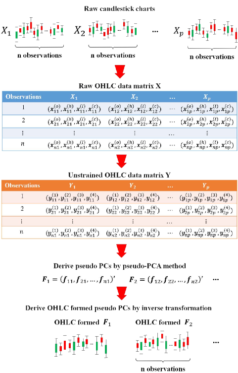
Fig. 2: The pseudo-PCA modelling framework for OHLC data

Algorithm 1   Pseudo-PCA procedure for OHLC data

1:$\textrm{{X}}=(\bm{X}_{1},\cdots,\bm{X}_{p})$ $\triangleright$ $n$ samples from the $p$-dimensional vector of OHLC data

2:$\textrm{{F}}=(\bm{F}_{1},\cdots,\bm{F}_{p})$ $\triangleright$ $\bm{F}_{j}$ is the $j$th pseudo-PC

3:Calculate the matrix of feature-based representations Y according to Equation (1) and (2).

4:Derive standardized Y according to Equation (14). For the sake of convenience, still record the standardized matrix as Y.

5:Calculate the correlation coefficient matrix $\bm{W}\in\mathbb{R}^{p\times p}$ of the standardized matrix Y. For the matrix $\bm{W}$, derive its first $m$ eigenvalues $\lambda_{1}\geq\lambda_{2}\geq\cdots\geq\lambda_{m}>0$, and the corresponding eigenvectors $\bm{u}_{1},\bm{u}_{2},...,\bm{u}_{m}$. According to Equation (15), the first $m$ pseudo-PCs $\bm{F}_{1},\bm{F}_{2},...,\bm{F}_{m}$ can be calculated.

6:After obtaining $\bm{F}_{h}=\left(\bm{f}_{1h},\bm{f}_{2h},\ldots,\bm{f}_{nh}\right)^{\prime}\in\mathbb{R}_{n}^{4}\;(h=1,2,\ldots,m)$, since each element$\bm{f}_{ih}=\left(f_{ih}^{(1)},f_{ih}^{(2)},f_{ih}^{(3)},f_{ih}^{(4)}\right)^{\prime}\in\mathbb{R}^{4}\;(1\leq i\leq n)$, the corresponding OHLC formed pseudo-principle components F can be obtained through Equation (4).

Finally, we realize the pseudo-PCA for OHLC data by extracting its feature information and successfully reduce the dimensionality of an OHLC data set with $n$ observations and $p$ variables to a new OHLC data set with $n$ observations and $m$ new components (pseudo-PCs), and $m\leq p$. In this process, the variance loss of the feature information matrix is minimal.

4 Simulations

The performance of pseudo-PCA is evaluated via finite sample simulation studies in term of the following two aspects: (1) the ability to remove redundant variables and reduce the dimensionality of raw data, and (2) the consistency of the estimated loadings of pseudo-PCs.

Here we assume that $p=6$ and the unconstrained OHLC data variable vector $\textrm{{Y}}=(\bm{Y}_{1},\bm{Y}_{2},\bm{Y}_{3},\bm{Y}_{4},\bm{Y}_{5},\bm{Y}_{6})$ satisfy that (1) each the unconstrained OHLC data variable $\bm{Y}_{j}$ is mean zero for $j=1,2,\cdots,6$; and (2) the correlation coefficient matrix $\bm{W_{\mathrm{Y}}}$ is set as following:

$$\bm{W_{\mathrm{Y}}}=\left(\begin{array}[]{cccccc}1&\frac{0.5^{2}}{2}&\frac{0.5^{2}}{3}&\frac{0.5^{2}}{4}&\frac{1.25}{\sqrt{5.5}}&\frac{0.5}{\sqrt{25.5}}\\ \frac{0.5^{2}}{2}&1&\frac{0.5^{2}}{6}&\frac{0.5^{2}}{8}&\frac{4.25}{2\sqrt{5.5}}&\frac{0.5}{2\sqrt{25.5}}\\ \frac{0.5^{2}}{3}&\frac{0.5^{2}}{6}&1&\frac{0.5^{2}}{12}&\frac{0.5}{3\sqrt{5.5}}&\frac{9.25}{3\sqrt{25.5}}\\ \frac{0.5^{2}}{4}&\frac{0.5^{2}}{8}&\frac{0.5^{2}}{12}&1&\frac{0.5}{4\sqrt{5.5}}&\frac{16.25}{4\sqrt{25.5}}\\ \frac{1.25}{\sqrt{5.5}}&\frac{4.25}{2\sqrt{5.5}}&\frac{0.5}{3\sqrt{5.5}}&\frac{0.5}{4\sqrt{5.5}}&1&\frac{2}{\sqrt{140.25}}\\ \frac{0.5}{\sqrt{25.5}}&\frac{0.5}{2\sqrt{25.5}}&\frac{9.25}{3\sqrt{25.5}}&\frac{16.25}{4\sqrt{25.5}}&\frac{2}{\sqrt{140.25}}&1\end{array}\right).\vspace*{-0.1cm}$$ (18)

Actually, from Equation (18), there are two redundant variables $\bm{Y}_{5}$ and $\bm{Y}_{6}$, i.e. $\bm{Y}_{5}=\bm{Y}_{1}+\bm{Y}_{2}$ and $\bm{Y}_{6}=\bm{Y}_{3}+\bm{Y}_{4}$. The sample sizes are $n=50,100,150,200$ with each case $300$ repeats, and we summary the performance of proposed procedure in term of two measurements: (1) the cumulative variance contribution rate of the first four pseudo-PCs; and (2) the mean absolute percentage error (MAPE) of the eigenvectors, i.e., $\operatorname{MAPE}_{j}=\frac{\left\|\widehat{\bm{u}}_{j}-\bm{u}_{j}\right\|}{\left\|\bm{u}_{j}\right\|}\times 100\%$ $(1\leq j\leq 6)$. For each criteria, we also report the empirical standard derivations.

The cumulative variance contribution rate of the first four pseudo-PCs is very stable with the change of sample size and always reaches 100.0%. Take $n=200$ as an example, Figure.3 shows the 100.0% explanatory capability of the first four pseudo-PCs. This verified the extraordinary ability of pseudo-PCA to remove redundant variables. Further, Table.1 shows the results of MAPE and its empirical standard derivations with different sample size. The estimation accuracy of PC5 and PC6 is relatively high and that of PC3 and PC4 is relatively low. The mean values of MAPE range from 13.2% to 27.9%, and its empirical standard derivations varies from 0.136 to 0.269, which are both within the acceptable range. Meanwhile, with the increase of sample size, MAPE and its empirical standard derivations show a decreasing trend, indicating that the estimated eigenvectors gradually converges to the theoretical values. These results identified the consistency between the estimated loadings of pseudo-PCs derived from the sample data and the theoretical values.

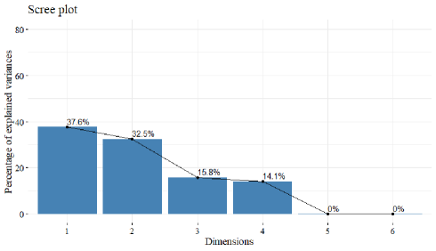
Fig. 3: Cumulative variance contribution plot of simulation with $n=200$

Table 1: Average of MAPE and its empirical standard deviation based on 300 repetitions

Sample size	PC1	PC2	PC3	PC4	PC5	PC6	Mean
$\mathrm{n}=50$	26.5%	28.5%	46.9%	47.1%	8.9%	9.3%	27.9%
	(0.308)	(0.301)	(0.320)	(0.318)	(0.185)	(0.184)	(0.269)
$\mathrm{n}=100$	14.1%	15.2%	34.8%	34.6%	8.2%	8.4%	19.2%
	(0.162)	(0.159)	(0.259)	(0.260)	(0.197)	(0.196)	(0.206)
$\mathrm{n}=150$	11.3%	12.6%	31.5%	31.6%	6.2%	6.4%	16.6%
	(0.141)	(0.139)	(0.226)	(0.225)	(0.163)	(0.162)	(0.176)
$\mathrm{n}=200$	8.9%	9.8%	25.3%	25.2%	5.0%	5.1%	13.2%
	(0.067)	(0.066)	(0.204)	(0.205)	(0.138)	(0.137)	(0.136)

5 Empirical analysis

In order to illustrate the effectiveness of the proposed pseudo-PCA, this paper extracts the OHLC data of he spot prices of $6$ common foods of $20$ important agricultural product markets in China from Wind (https://www.wind.com.cn/). The $6$ OHLC data variables include: beef $(CNY/kg)$, lamb $(CNY/kg)$, pork $(CNY/kg)$, cucumber $(CNY/kg)$, potato $(CNY/kg)$, and onion $(CNY/kg)$. The observed dates range from $1/1/2019$ to $31/12/2019$, and we use the first price recorded in the time period as the open price, last price recorded as the close price, and highest/lowest price that appears during the time period as the high/low price.

The original OHLC data matrix X can be referred to Table.4 in Appendix.B. First, the standardized feature information matrix Y is derived and shown in Table.5 in Appendix.B. Conduct pseudo-PCA modelling on the standardized feature information matrix Y, the corresponding eigenvalues (EV), variance contribution rate (VCR), and cumulative contribution to the variance (CVCR) of the $6$ extracted pseudo-PCs are shown in Table.2. The cumulative contribution rate to the variance of the first two pseudo-PCs reaches 57.4$\%$, and that of the first three pseudo-PCs reaches 73.2$\%$. This implies that the pseudo-principle components represent the information of the original data matrix well. The corresponding variance cumulative contribution plot is shown in Figure.4.

Table 2: The EV, VCR and CVCR of the 6 pseudo-PCs

pseudo-PCs	EV	VCR	CVCR
PC1	2.065	0.344	0.344
PC2	1.376	0.229	0.574
PC3	0.950	0.158	0.732
PC4	0.705	0.118	0.849
PC5	0.619	0.103	0.953
PC6	0.285	0.048	1.000

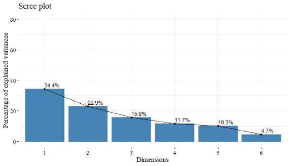
Fig. 4: Cumulative variance contribution plot

Furthermore, the loading matrix of the first two pseudo-PCs is shown in Table.3. The expressions of these two pseudo-PCs are:

PC1 $$= 0.222\otimes\bm{Y}_{1}\oplus 0.115\otimes\bm{Y}_{2}\oplus 0.248\otimes\bm{Y}_{3}\oplus 0.543\otimes\bm{Y}_{4}\oplus 0.599\otimes\bm{Y}_{5}\oplus 0.471\otimes\bm{Y}_{6}$$

PC2 $$= 0.563\otimes\bm{Y}_{1}\oplus 0.687\otimes\bm{Y}_{2}\oplus 0.330\otimes\bm{Y}_{3}\ominus 0.199\otimes\bm{Y}_{4}\ominus 0.129\otimes\bm{Y}_{5}\ominus 0.213\otimes\bm{Y}_{6}$$

Table 3: The loading matrix of the first two pseudo-PCs

Feature information variables	PC1	PC2
Beef   ($\bm{Y}_{1}$)	0.222	0.563
Lamb   ($\bm{Y}_{2}$)	0.115	0.687
Pork   ($\bm{Y}_{3}$)	0.248	0.330
Cucumber   ($\bm{Y}_{4}$)	0.543	-0.199
Potato   ($\bm{Y}_{5}$)	0.599	-0.129
Onion   ($\bm{Y}_{6}$)	0.471	-0.213

The correlation between the first two pseudo-principle components and feature information variables are clearly visualized through Figure.5. In Figure.5, positively related variables are close to each other, while negatively related variables are divergent. The lengths of the arrows represent the information quality of different variables. It is observed that the loading factors’ absolute values of the PC1 on cucumbers, potatoes, and onions are relatively large, which can be called a ‘Vegetable’ factor. The loading factors’ absolute values of the PC2 on beef, lamb, and pork are comparatively large, and it can be called a ‘Meat’ factor.

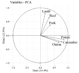
Fig. 5: Correlation of the first two pseudo-PCs and the feature information variables

According to Equation (15), the scores of the first two pseudo-PCs can be calculated, and the corresponding OHLC formed data can be derived by using Equation (4). The results are shown in Figure.6 and Figure.7, where the abbreviations of the 20 markets are used (the corresponding full name can be referred to Table.6 in Abbreviation.C).

Based on the OHLC formed pseudo-PC scores, we can observe the size and fluctuation of the original data during the observation period. For instance, (1) For the OHLC data converted from the first pseudo-PC scores (‘Vegetable’ factor), it is observed that the open, high, low, and open prices of Zhangjiajie and Xinyu have always been at a high level. This means that the prices of cucumbers, potatoes, and onions in these two cities maintained a high level through 2019. At the same time, the difference between the low price and high price of Zhangjiajie is relatively large, indicating that the prices of cucumbers, potatoes, and onions in Zhangjiajie experienced great fluctuations in 2019. While the difference between the upper and lower bounds of Xinyang is very small, corresponding to the prices of ‘Vegetable’ in Xinyang were very stable in 2019. Markets with green-body OHLC data had a relatively low comprehensive price for cucumbers, potatoes, and onions at the beginning of 2019 and relatively high comprehensive price at the end of 2019. While the comprehensive price for cucumbers, potatoes, and onions of the red-body markets tended to open higher, and finish lower. (2) For the OHLC data transformed by the second pseudo-PC scores (‘Meat’ factor), we see that the open price of Zhangjiajie is at the medium level. This indicates that at the beginning of 2019, the prices of beef, lamb, and pork in Zhangjiajie were not high. However, its candlestick stretches to the highest and lowest among all the markets, suggesting that the ‘Meat’ price in Zhangjiajie experienced great fluctuations in 2019, resulting in the prices appearing extremely high and extremely low. On the other hand, the four-dimensional data of Jiangsu are very small, indicating that its price of ‘Meat’ remained stable in 2019, which corresponds to the original lamb price of Jiangsu remained at $58\;CNY/kg$ throughout the year.

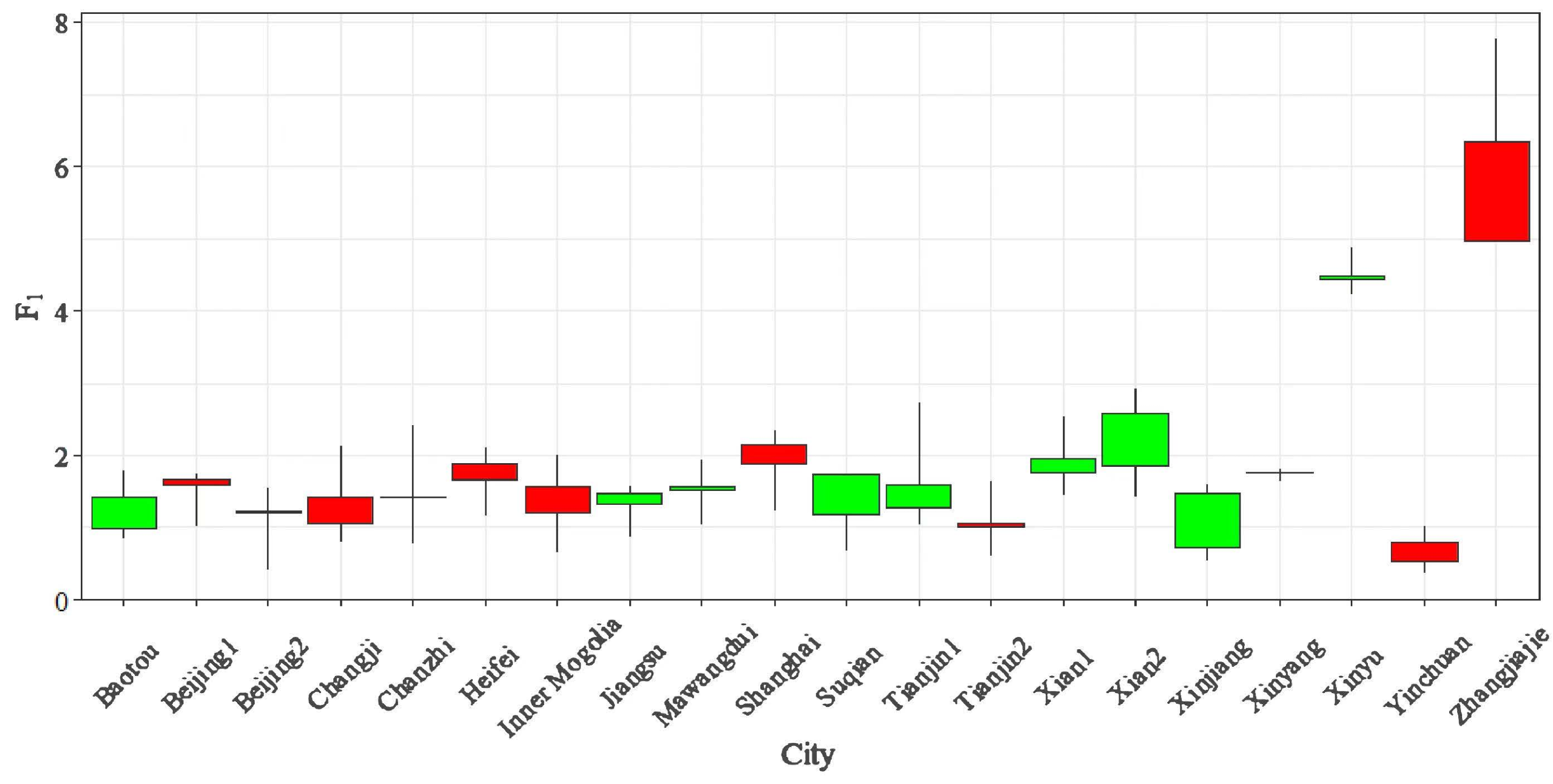
Fig. 6: The first OHLC formed pseudo-PC scores

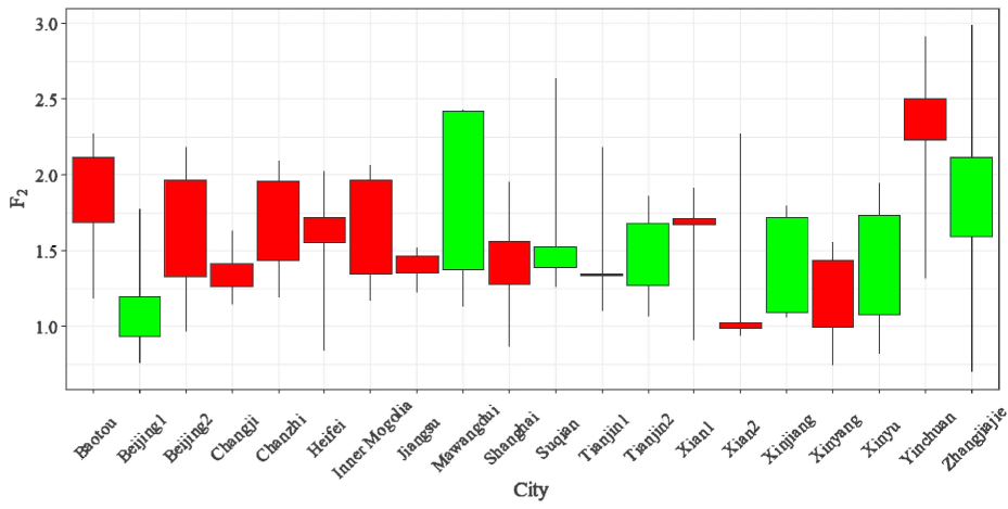
Fig. 7: The second OHLC formed pseudo-PC scores

It is important to mention that an eigenvector uniquely corresponds to one pseudo-PC and one transformed OHLC data. However, for each eigenvalue of the standardized feature information matrix Y, there are two corresponding eigenvectors, which are mutually opposite vectors. The difference in sign does not affect the orthogonal and normalized requirements in Theorem.1, they are both feasible solutions. Paradoxically, the pseudo-PCs corresponding to these two eigenvectors are different, and the restored OHLC formed pseudo-principle component scores are also different. In order to enhance the interpretability of the pseudo-PCA for OHLC data, it is recommended that the eigenvector is selected by the following rule. If the eigenvector has the largest absolute loading values on the feature information variables, such as $\bm{Y}_{1},\bm{Y}_{2}$ and $\bm{Y}_{3}$, then select the eigenvector that has positive loading values on $\bm{Y}_{1},\bm{Y}_{2}$ and $\bm{Y}_{3}$. This way, a relationship is established. The original data size, feature information size, pseudo-PC scores, and OHLC formed pseudo-PC scores are all positively related to each other. The advantage of this practice lies in the original data size and can be easily analyzed through the final comprehensive OHLC formed pseudo-principle component scores. For instance, in this article, we see that the loading values of the ‘Vegetable’ factor for cucumbers, potatoes, and onions are all positive; the loading values of the ‘Meat’ factor for beef, lamb, and pork are also all positive.

6 Conclusions

As more OHLC data is collected, the demand for dimension reduction of the OHLC data emerges. Inspired by the various PCA methods applied for interval data, this paper proposed a novel modus for characterizing features of OHLC data and built a unique $\mathbb{R}_{n}^{4}$ space containing the feature-based representations accordingly. The new method of representing the OHLC data can eliminate the inherent constraints of OHLC data and transition between the original OHLC data and its feature-based representations freely. In the unique $\mathbb{R}_{n}^{4}$ space, we defined the linear operations and inner product operation and deduced the pseudo-PCA method for OHLC data under this new algebraic framework. The pseudo-PCA has high visibility and high interpretability, which can effectively identify important information and perform dimension reduction. Therefore, reducing the dimensionality of an OHLC data set with $n$ observations and $p$ variables to a new OHLC data set with $n$ observations and $m$ components is achieved, and $m\leq p$. The effectiveness, robustness and interpretability of the pseudo-PCA is examined by finite simulations and empirical experiment.

The OHLC formed pseudo-PCs derived from pseudo-PCA still hold the constraints of OHLC data, which maintains the original format of the raw data and provides significant convenience for the subsequent establishment of econometric or machine learning models. Through the OHLC formed pseudo-PCs, one can observe the size and the fluctuation of certain original data variables during the observation period. Furthermore, the OHLC formed pseudo-PCs can be presented in the format of the candlestick chart, which helps people obtain information easily. Overall, this paper provides a novel feature-based representation method for OHLC data and enriches the existing literature on PCA methods.

For scalar data, the Singular Spectrum Analysis (SSA) is applied instead of PCA when performing dimension reduction of panel data. Similarly, we may further propose the new pseudo-SSA approach to address the time-series OHLC data set, which can be an interesting research direction in the future. Besides, exploring new feature extraction methods for more generalized interval-valued data is significant. For instance, many types of data (i.e., daily temperatures, companies’ profits, and stock returns) hold intervals and own values between the upper and lower boundaries (low value may be negative) while not belonging to OHLC data.

Declarations

Funding

This study was funded by the National Natural Science Foundation of China (grant numbers. $71420107025$, $11701023$).

Conflicts of interest

Author Wenyang Huang declares that he has no conflict of interest. Author Huiwen Wang declares that she has no conflict of interest. Author Shanshan Wang declares that she has no conflict of interest.

Ethical approval

This article does not contain any studies with human participants or animals performed by any of the authors.

Availability of data and material

The spot data is downloaded form a financial server called Wind. The data can be uploaded as required.

Code availability

This paper applies custom R code and can be uploaded as required.

Appendix A A Proof of Proposition.1

Proposition 1. For any two OHLC data $\bm{x}$ and $\tilde{\bm{x}}$ with their corresponding feature-based representations $\bm{y}$ and $\tilde{\bm{y}}$, then it holds $\bm{x}=\tilde{\bm{x}}$ if and only if $\bm{y}=\tilde{\bm{y}}$ holds.

$\bm{Proof:}$

Obviously, $\bm{x}=\tilde{\bm{x}}$ implies $\bm{y}=\tilde{\bm{y}}$ from Definition.2. It suffices to prove that if $\bm{y}=\tilde{\bm{y}}$, then $\bm{x}=\tilde{\bm{x}}$. In fact, since $\bm{y}=\left(y^{(1)},y^{(2)},y^{(3)},y^{(4)}\right)^{\prime}$ and $\tilde{\bm{y}}=\left(\tilde{y}^{(1)},\tilde{y}^{(2)},\tilde{y}^{(3)},\tilde{y}^{(4)}\right)^{\prime}$, $\bm{y}=\tilde{\bm{y}}$ implies that $y^{(j)}=\tilde{y}^{(j)},\;j=1,2,3,4$.

First, $y^{(1)}=\text{ln}x^{(l)}$, $\tilde{y}^{(1)}=\text{ln}\tilde{x}^{(l)}$ $\Rightarrow$ $y^{(1)}=\tilde{y}^{(1)}$ implies $x^{(l)}=\tilde{x}^{(l)}$ (1).

Second, $y^{(2)}=\text{ln}(x^{(h)}-x^{(l)})$, then $y^{(2)}=\tilde{y}^{(2)}$ together with $x^{(l)}=\tilde{x}^{(l)}$ implies that $\tilde{y}^{(2)}=\text{ln}(\tilde{x}^{(h)}-\tilde{x}^{(l)})$, $x^{(h)}=\tilde{x}^{(h)}$ (2).

Third, $y^{(3)}=\tilde{y}^{(3)}$ and $y^{(4)}=\tilde{y}^{(4)}$ yield $\lambda^{(o)}=\tilde{\lambda}^{(o)}$ and $\lambda^{(c)}=\tilde{\lambda}^{(c)}$.

Thus, $x^{(o)}=\lambda^{(o)}x^{(h)}+(1-\lambda^{(o)})x^{(l)}=\tilde{\lambda}^{(o)}\tilde{x}^{(h)}+(1-\tilde{\lambda}^{(o)})\tilde{x}^{(l)}=\tilde{x}^{(o)}$ (3); $x^{(c)}=\lambda^{(c)}x^{(h)}+(1-\lambda^{(c)})x^{(l)}=\tilde{\lambda}^{(c)}\tilde{x}^{(h)}+(1-\tilde{\lambda}^{(c)})\tilde{x}^{(l)}=\tilde{x}^{(c)}$ (4).

Therefore, $\bm{y}=\tilde{\bm{y}}$ $\Rightarrow$ $\bm{x}=\tilde{\bm{x}}$. As desired.

$\bm{Proof\;up}$

Appendix B B Proof of Proposition.2

Proposition 2. If the feature information variables $\bm{Y}_{1},\bm{Y}_{2},\ldots,\bm{Y}_{p}$ are standardized, the first $m$ pseudo-principle components $\bm{F}_{h}\in\mathbb{R}_{n}^{4}\;(1\leq h\leq m,m\leq p)$ derived from the pseudo-PCA satisfy the following properties:
(1)  The sample mean of $\bm{F}_{m}$ is equal to $0$, that is, $\overline{\bm{F}}_{h}=\mathbf{0}\in\mathbb{R}^{4}$;
(2)  The sample variance of $\bm{F}_{m}$ is equal to $\lambda_{h}$, namely, $\operatorname{Var}\left(\bm{F}_{h}\right)=\lambda_{h}$;
(3)  For any $\bm{F}_{h},\bm{F}_{k}\in\mathbb{R}_{n}^{4}$, if $h\neq k$, their sample covariance $Cov(\bm{F}_{h},\bm{F}_{k})=0$;
(4)  $\max\sum_{h=1}^{m}Var(\bm{F}_{h})=p.$

$\bm{Proof:}$

In regard to conclusion (1), because it is assumed that $\bm{Y}_{1},\bm{Y}_{2},\ldots,\bm{Y}_{p}$ have been standardized, there is $\overline{\bm{Y}}_{j}=\mathbf{0},\;j=1,2,\ldots,p$. Since $\bm{F}_{h}$ is a linear combination of $\bm{Y}_{1},\bm{Y}_{2},\ldots,\bm{Y}_{p}$, it is easy to deduce:

$$\overline{\bm{F}}_{h}=E(\bm{F}_{h})=E(u_{h1}\otimes\bm{Y}_{1}\oplus u_{h2}\otimes\bm{Y}_{2}\oplus\cdots\oplus u_{hp}\otimes\bm{Y}_{p})$$

$$=u_{h1}\times E(\bm{Y}_{1})+u_{h2}\times E(\bm{Y}_{2})+\cdots+u_{hp}\times E(\bm{Y}_{p})$$

$$=u_{h1}\times(0,0,0,0)^{\prime}+u_{h2}\times(0,0,0,0)^{\prime}+\cdots+u_{hp}\times(0,0,0,0)^{\prime}$$

$$=(0,0,0,0)^{\prime}+(0,0,0,0)^{\prime}+\cdots+(0,0,0,0)^{\prime}$$

$$=(0,0,0,0)^{\prime}$$

As for conclusion (2), since $\bm{u}_{h}^{\prime}\bm{u}_{h}=1$, there is:

$\operatorname{Var}\left(\bm{F}_{h}\right)=\frac{1}{n}\left(\bm{F}_{h},\bm{F}_{h}\right)_{\mathbb{R}_{n}^{4}}=\bm{u}_{h}^{\prime}\bm{W}\bm{u}_{h}=\bm{u}_{h}^{\prime}\lambda_{h}\bm{u}_{h}=\lambda_{h}$

The proof of conclusion (3) is similar. For $h\neq k$, because of $\bm{u}_{h}$ and $\bm{u}_{k}$ are orthogonal, so:

$\operatorname{Cov}\left(\bm{F}_{h},\bm{F}_{k}\right)=\frac{1}{n}\left(\bm{F}_{h},\bm{F}_{k}\right)_{\mathbb{R}_{n}^{4}}=\bm{u}_{h}^{\prime}\bm{W}\bm{u}_{k}=\bm{u}_{h}^{\prime}\lambda_{k}\bm{u}_{k}=0$

When it comes to conclusion (4), record matrix $\bm{U}=(\bm{u}_{1},\bm{u}_{2},\ldots,\bm{u}_{p})$, which is an orthogonal matrix, and mark the diagonal matrix as $\bm{\Lambda}=\operatorname{diag}\left(\lambda_{1},\lambda_{2},\ldots,\lambda_{p}\right)$, because there is:

$\bm{U}^{\prime}\bm{W}\bm{U}=\bm{\Lambda}$

The correlation coefficient matrix $\bm{W}$ and $\bm{\Lambda}$ are two similar square matrices. The traces of these two matrices are:

$\operatorname{tr}(\bm{W})=p,\quad\operatorname{tr}(\bm{\Lambda})=\sum_{h=1}^{p}\lambda_{h}$

Because the traces of similar square matrices are equal, and $Var(\bm{F}_{h})=\lambda_{h}\;(h=1,2,\ldots,p)$, we can derive the conclusion (4): $\sum_{h=1}^{p}Var(\bm{F}_{h})=p$.

$\bm{Proof\;up}$

Appendix C C Data used in this paper

Table 4: Raw OHLC data

Markets	Beef	Lamb	Pork	Cucumber	Potato	Onion
Baotou Youyi market vegetable wholesale market	(62, 72, 58, 72)’	(57, 64, 52, 60)’	(22, 56, 20, 44)’	(5, 9, 1.4, 5)’	(1.6, 3, 1.5, 2)’	(1.4, 3, 1.4, 3)’
Beijing Dayanglu Agricultural and Sideline Products Market Co., Ltd	(53.5, 66.5, 52, 66)’	(47, 54.5, 46.98, 54)’	(15.8, 49.75, 11.5, 39)’	(6.4, 9, 2, 6.6)’	(2.6, 2.8, 1.8, 2.4)’	(1.9, 3.3, 1.3, 3.2)’
Beijing Xinfadi Agricultural Products Co., Ltd	(54.25, 67.5, 51.6, 65.75)’	(52.8, 56.9, 42.8, 54.8)’	(15.65, 50.25, 11.5, 40.5)’	(4, 9, 1.2, 4.3)’	(1.95, 3, 0.9, 2.3)’	(1.3, 2.3, 0.95, 2.3)’
Changji Yuanfeng Agricultural and Sideline Products Trading Market Co., Ltd	(60, 60.5, 56, 59)’	(53, 61.5, 53, 60)’	(19, 48.5, 18, 37)’	(6, 12, 1.5, 7.5)’	(1.8, 4, 1.5, 2)’	(1.8, 3, 1, 2)’
Hefei Zhougudui Agricultural Products Wholesale Market Co., Ltd	(62, 74.5, 58, 74.5)’	(61, 70, 54, 64)’	(14.9, 43.14, 12.12, 36)’	(5.5, 10, 2, 7)’	(2.9, 3.7, 2.2, 2.7)’	(1.8, 2.8, 1.2, 2.1)’
Jiangsu Lingjiatang Market Development Co., Ltd	(70, 80, 58, 80)’	(58, 58, 58, 58)’	(22, 56.5, 19.8, 45)’	(5.6, 6.6, 1.4, 4.5)’	(1.8, 3.4, 1.6, 2.2)’	(1.4, 3.6, 1.4, 3.6)’
Mawangdui Agricultural Products Co., Ltd	(66, 86, 66, 86)’	(62, 73, 61, 73)’	(18.8, 54, 16.9, 46)’	(4, 7, 1.8, 3)’	(2.6, 3.2, 1.6 2.6)’	(1.8, 4.2, 1.3, 3.3)’
Inner Mongolia Dongwayao Agricultural and Sideline Products Wholesale Market Co., Ltd	(62, 66.2, 56, 64)’	(54, 60.5, 50, 56)’	(24, 60, 18, 48)’	(5, 10, 1.2, 5.6)’	(2.2, 3.6, 1.2, 2.2)’	(1.6, 3.1, 1.5, 2.8)’
Shanghai Jiangyang Agricultural Products Logistics Co., Ltd	(63, 80.4, 60, 79.2)’	(56.1, 62.8, 54.4, 61.5)’	(19.39, 52.87, 13.14, 43.07)’	(7.2, 9.8, 2, 6.2)’	(2.5, 3.4, 2, 2.4)’	(2.2, 4.1, 1.6, 4.1)’
Tianjin Hanjiashu Haijixing Agricultural Products Logistics Co., Ltd	(57, 72, 55, 70)’	(74, 82, 70, 78)’	(17.3, 60, 17.3, 41)’	(4.8, 10.2, 2, 5.7)’	(2.3, 4, 1.4, 2.4)’	(1.6, 4, 1.3, 3.5)’
Tianjin Jinyuanbao Binhai Agricultural Products Trading Market	(52, 58, 50, 58)’	(48, 55, 48, 55)’	(17.5, 61, 16, 43)’	(4.3, 8.3, 1.2, 4.8)’	(2.3, 3.6, 1.3, 2)’	(1.3, 2.7, 1.2, 2.1)’
Xian Xinbeicheng Agricultural and Sideline Products Trading Market Management Co., Ltd	(58.2, 68.2, 55, 68)’	(58, 64.2, 51, 64)’	(19.4, 52, 18, 42)’	(5.2, 11, 2.2, 6)’	(2.2, 3.6, 2, 2.6)’	(1.8, 3.4, 1.6, 3)’
Xian Zhuque Agricultural Products Market Co., Ltd	(60, 76.01, 56, 70)’	(60, 76, 60, 62)’	(17, 56, 17, 42)’	(6, 11, 2, 9)’	(2.6, 5, 2, 3)’	(2.61, 3, 2, 3)’
Xinjiang Xibulvzhu Fruit and Vegetable Co., Ltd.	(55, 63, 55, 63)’	(52, 62, 52, 62)’	(15.5, 47, 12.5, 39)’	(5.5, 11, 1, 7.5)’	(1.8, 3, 1.5, 2.2)’	(1.3, 3, 1.2, 3)’
Xinyu Youzhi Agricultural Products Wholesale Market	(63.7, 80.1, 63.7, 80)’	(63.9, 68, 60, 66)’	(23.4, 58.5, 22.4, 56)’	(4.8, 10, 3.4, 6)’	(4.2, 5, 3.8, 4.1)’	(4.5, 4.8, 3.6, 4.2)’
Xinyang Yunong Agricultural Products Sales Co., Ltd	(45, 48, 42, 47)’	(55, 57, 52, 56)’	(19, 44, 16.5, 39)’	(4.3, 6.1, 3.1, 5.5)’	(2, 2.6, 2, 2.3)’	(2.1, 2.2, 1.3, 1.6)’
Suqian Nancaishi Agricultural and Sideline Products Wholesale Market Management Co., Ltd	(60.95, 75, 60, 74)’	(56.05, 78, 56, 77)’	(17.68, 54, 17.02, 44)’	(4.31, 7.95, 1.02, 7.5)’	(2.7, 3.85, 2, 3.7)’	(1.58, 2.82, 1.02, 2.8)’
Yinchuan Beihuan Vegetables and Fruits Comprehensive Wholesale Market Management Co., Ltd	(54.6, 69, 51, 68)’	(57.4, 66, 50, 64)’	(19.2, 56, 16, 46)’	(3.7, 9.04, 0.76, 5.8)’	(1.52, 2.16, 1.2, 1.5)’	(1.2, 1.6, 0.86, 0.92)’
Zhangjiajie Yongding District Market Management Service Center	(56, 98, 54, 80)’	(56, 94, 54, 74)’	(27, 70, 23, 46)’	(6, 10, 4, 4.2)’	(5, 8, 4, 4)’	(7, 10, 4, 4)’
Changzhi Zifang Agricultural Products Comprehensive Trading Market Co., Ltd	(64, 74, 60, 72)’	(72, 74, 66, 72)’	(18, 64, 16, 50)’	(4.8, 12, 1.6, 5.4)’	(1.8, 3.2, 1.4, 1.8)’	(1.4, 3.6, 1, 3.6)’

Table 5: Feature-based representations

Markets	Beef	Lamb	Pork	Cucumber	Potato	Onion
Baotou Youyi market vegetable wholesale market	(0.03, 0, 0.63, 1.2)’	(-0.02, 0.13, 0.89, -0.71)’	(0.27, -0.06, 0.36, -0.34)’	(-0.27, 0.05, 0.22, -0.29)’	(-0.13, -0.13, -1.67, -0.02)’	(0, -0.05, -2.58, 1.21)’
Beijing Dayanglu Agricultural and Sideline Products Market Co., Ltd	(-0.05, 0.02, -0.2, 0.03)’	(-0.07, -0.11, -1.92, 0.27)’	(-0.47, 0.02, 1.39, -0.01)’	(0.25, -0.07, 1.14, 0.81)’	(0.04, -0.52, 2.22, 1.05)’	(-0.05, 0.07, 0.27, 0.8)’
Beijing Xinfadi Agricultural Products Co., Ltd	(-0.05, 0.08, 0.17, -0.81)’	(-0.12, 0.21, 1.51, -0.18)’	(-0.47, 0.04, 1.32, 0.2)’	(-0.49, 0.09, -0.48, -0.74)’	(-0.63, 0.2, 0.88, 1.32)’	(-0.24, -0.17, 0.13, 1.42)’
Changji Yuanfeng Agricultural and Sideline Products Trading Market Co., Ltd	(0, -0.77, 2.65, -1.75)’	(-0.01, -0.04, -1.67, -0.28)’	(0.13, -0.28, -0.38, -0.59)’	(-0.17, 0.52, -0.05, 0.29)’	(-0.13, 0.36, -1.05, -0.69)’	(-0.21, 0.07, 0.55, -1.07)’
Hefei Zhougudui Agricultural Products Wholesale Market Co., Ltd	(0.03, 0.11, 0.48, 1.4)’	(0, 0.27, 0.93, -0.8)’	(-0.4, -0.26, 1.05, 0.36)’	(0.25, 0.12, 0, 0.61)’	(0.24, -0.13, 0.75, -0.02)’	(-0.1, -0.07, 0.49, -0.91)’
Jiangsu Lingjiatang Market Development Co., Ltd	(0.03, 0.3, 1.37, 2.27)’	(0.03, -2.08, 1.09, -1.03)’	(0.26, -0.04, 0.47, -0.21)’	(-0.27, -0.5, 2.46, 0.43)’	(-0.07, 0.05, -1.13, -0.02)’	(-0.04, 0.15, -1.21, 2.6)’
Mawangdui Agricultural Products Co., Ltd	(0.11, 0.24, -2.34, 1.78)’	(0.06, 0.13, -0.15, 4.49)’	(0.05, -0.02, 0.24, 0.47)’	(0.1, -0.5, -0.08, -1.89)’	(-0.07, -0.07, 1.38, 1.15)’	(-0.05, 0.3, -0.18, -0.56)’
Inner Mongolia Dongwayao Agricultural and Sideline Products Wholesale Market Co., Ltd	(0, -0.22, 1.49, -1.34)’	(-0.04, 0.06, 0.82, -0.91)’	(0.13, 0.15, 1.76, -0.04)’	(-0.49, 0.26, -0.03, -0.13)’	(-0.35, 0.32, 0.56, 0.33)’	(0.04, -0.07, -0.9, -0.14)’
Shanghai Jiangyang Agricultural Products Logistics Co., Ltd	(0.05, 0.24, 0.07, -0.35)’	(0, -0.05, 0.37, -0.2)’	(-0.29, 0.07, 1.91, 0.23)’	(0.25, 0.09, 1.38, 0.09)’	(0.14, -0.2, 0.31, -0.23)’	(0.09, 0.23, 0.05, 0.97)’
Tianjin Hanjiashu Haijixing Agricultural Products Logistics Co., Ltd	(-0.01, 0.12, -0.1, -0.86)’	(0.13, 0.13, 0.71, -0.71)’	(0.08, 0.17, -5.64, -0.97)’	(0.25, 0.16, -0.59, -0.42)’	(-0.2, 0.4, 0.27, 0.2)’	(-0.05, 0.26, -0.51, -0.13)’
Tianjin Jinyuanbao Binhai Agricultural Products Trading Market	(-0.07, -0.38, 0.5, 0.75)’	(-0.06, -0.13, -1.91, 1.23)’	(-0.03, 0.24, -0.36, -0.72)’	(-0.49, -0.05, 0, -0.09)’	(-0.27, 0.28, 0.63, -0.15)’	(-0.1, -0.12, -0.86, -0.81)’
Xian Xinbeicheng Agricultural and Sideline Products Trading Market Management Co., Ltd	(-0.01, -0.05, 0.49, 0.6)’	(-0.03, 0.18, 1.12, 1.04)’	(0.13, -0.14, -0.06, -0.09)’	(0.39, 0.26, -0.59, -0.53)’	(0.14, -0.07, -1, 0.16)’	(0.09, 0, -0.51, -0.27)’
Xian Zhuque Agricultural Products Market Co., Ltd	(0, 0.23, 0.32, -1.64)’	(0.05, 0.28, -1.89, -2.02)’	(0.05, 0.05, -4.12, -0.48)’	(0.25, 0.3, 0.04, 1.69)’	(0.14, 0.54, -0.46, -0.02)’	(0.23, -0.37, 1.08, 2.13)’
Xinjiang Xibulvzhu Fruit and Vegetable Co., Ltd.	(-0.01, -0.38, -3.48, 2.35)’	(-0.02, 0.04, -2.37, 1.83)’	(-0.36, -0.12, 1.01, 0.34)’	(-0.76, 0.45, 0.08, 0.77)’	(-0.13, -0.13, -0.46, 0.52)’	(-0.1, 0.02, -1.01, 1.01)’
Xinyu Youzhi Agricultural Products Wholesale Market	(0.09, 0.1, -2.93, 1.22)’	(0.05, -0.07, 1.03, -0.5)’	(0.43, -0.06, -0.61, 2.23)’	(1.02, -0.16, -1.54, -0.76)’	(0.77, -0.35, 0.21, -0.41)’	(0.6, -0.26, 1.51, -1.07)’
Xinyang Yunong Agricultural Products Sales Co., Ltd	(-0.19, -0.58, 1.25, -1.13)’	(-0.02, -0.31, 1.26, -0.36)’	(0.02, -0.42, 1.07, 0.75)’	(0.89, -1.31, -0.22, 1.89)’	(0.12, -0.94, -1.54, 0.8)’	(-0.05, -0.44, 2.13, -1.51)’
Suqian Nancaishi Agricultural and Sideline Products Wholesale Market Management Co., Ltd	(0.05, 0.04, -0.56, -0.44)’	(0.02, 0.43, -2, 0.47)’	(0.06, -0.03, -1.22, 0.07)’	(-0.73, -0.09, 0.22, 3.75)’	(0.14, 0.07, 0.4, 3)’	(-0.2, 0, 0.31, 1.77)’
Yinchuan Beihuan Vegetables and Fruits Comprehensive Wholesale Market Management Co., Ltd	(-0.06, 0.16, 0.32, -0.31)’	(-0.04, 0.27, 0.98, -0.08)’	(-0.03, 0.08, 0.89, 0.21)’	(-1.16, 0.17, -0.5, 0.51)’	(-0.35, -0.56, 0.21, -0.11)’	(-0.31, -0.56, 0.71, -2.6)’
Zhangjiajie Yongding District Market Management Service Center	(-0.02, 0.76, -0.79, -1.96)’	(0, 0.73, -0.42, -1.06)’	(0.46, 0.3, 0.98, -1.33)’	(1.26, -0.3, -0.64, -5.04)’	(0.81, 0.82, -0.18, -6.31)’	(0.66, 0.77, 0.82, -4.36)’
Changzhi Zifang Agricultural Products Comprehensive Trading Market Co., Ltd	(0.05, -0.01, 0.64, -1.01)’	(0.1, -0.07, 1.61, -0.5)’	(-0.03, 0.33, -0.05, -0.08)’	(-0.07, 0.51, -0.81, -0.94)’	(-0.2, 0.05, -0.33, -0.56)’	(-0.21, 0.24, -0.28, 1.5)’

Appendix D D Abbreviations

Table 6: Markets’ full name-abbreviated comparison table

Markets	Abbreviations
Baotou Youyi market vegetable wholesale market	Baotou
Beijing Dayanglu Agricultural and Sideline Products Market Co., Ltd	Beijing1
Beijing Xinfadi Agricultural Products Co., Ltd	Beijing2
Changji Yuanfeng Agricultural and Sideline Products Trading Market Co., Ltd	Changji
Hefei Zhougudui Agricultural Products Wholesale Market Co., Ltd	Hefei
Jiangsu Lingjiatang Market Development Co., Ltd	Jiangsu
Mawangdui Agricultural Products Co., Ltd	Mawangdui
Inner Mongolia Dongwayao Agricultural and Sideline Products Wholesale Market Co., Ltd	Inner Mongolia
Shanghai Jiangyang Agricultural Products Logistics Co., Ltd	Shanghai
Tianjin Hanjiashu Haijixing Agricultural Products Logistics Co., Ltd	Tianjin1
Tianjin Jinyuanbao Binhai Agricultural Products Trading Market	Tianjin2
Xian Xinbeicheng Agricultural and Sideline Products Trading Market Management Co., Ltd	Xian1
Xian Zhuque Agricultural Products Market Co., Ltd	Xian2
Xinjiang Xibulvzhu Fruit and Vegetable Co., Ltd.	Xinjiang
Xinyu Youzhi Agricultural Products Wholesale Market	Xinyu
Xinyang Yunong Agricultural Products Sales Co., Ltd	Xinyang
Suqian Nancaishi Agricultural and Sideline Products Wholesale Market Management Co., Ltd	Suqian
Yinchuan Beihuan Vegetables and Fruits Comprehensive Wholesale Market Management Co., Ltd	Yinchuan
Zhangjiajie Yongding District Market Management Service Center	Zhangjiajie
Changzhi Zifang Agricultural Products Comprehensive Trading Market Co., Ltd	Changzhi

References

- Abdi and Williams (2010) Hervé Abdi and Lynne Williams. Principal component analysis. Wiley Interdisciplinary Reviews: Computational Statistics, 2:433 – 459, 2010.
- Arroyo et al. (2011) Javier Arroyo, Rosa Espínola, and Carlos Maté. Different approaches to forecast interval time series: a comparison in finance. Computational Economics, 37(2):169–191, 2011.
- Brito and Duarte Silva (2012) Paula Brito and A Pedro Duarte Silva. Modelling interval data with normal and skew-normal distributions. Journal of Applied Statistics, 39(1):3–20, 2012.
- Brown et al. (2002) Philip Brown, Angeline Chua, and Jason Mitchell. The influence of cultural factors on price clustering: Evidence from asia–pacific stock markets. Pacific-Basin Finance Journal, 10(3):307–332, 2002.
- Cao and Tay (2003) Li-Juan Cao and Francis Eng Hock Tay. Support vector machine with adaptive parameters in financial time series forecasting. IEEE Transactions on neural networks, 14(6):1506–1518, 2003.
- Cazes et al. (1997) Pierre Cazes, Ahlame Chouakria, Edwin Diday, and Yves Schektman. Extension de l’analyse en composantes principales à des données de type intervalle. Revue de Statistique appliquée, 45(3):5–24, 1997.
- Cervelló-Royo et al. (2015) Roberto Cervelló-Royo, Francisco Guijarro, and Karolina Michniuk. Stock market trading rule based on pattern recognition and technical analysis: Forecasting the djia index with intraday data. Expert systems with Applications, 42(14):5963–5975, 2015.
- Cheung (2007) Yin-Wong Cheung. An empirical model of daily highs and lows. International Journal of Finance & Economics, 12(1):1–20, 2007.
- Chmielewski et al. (2015) Leszek Chmielewski, Maciej Janowicz, Joanna Kaleta, and Arkadiusz Orłowski. Pattern recognition in the japanese candlesticks. In Soft computing in computer and information science, pages 227–234. Springer, 2015.
- Chouakria et al. (2000) A Chouakria, P Cazes, E Diday, and HH Bock. Symbolic principal component analysis. Analysis of Symbolic Data, ed. HH Bock, and E. Diday, pages 200–212, 2000.
- Cohen et al. (2019) Naftali Cohen, Tucker Balch, and Manuela Veloso. Trading via image classification. arXiv preprint arXiv:1907.10046, 2019.
- De Nard et al. (2020) Gianluca De Nard, Robert F Engle, Olivier Ledoit, and Michael Wolf. Large dynamic covariance matrices: enhancements based on intraday data. University of Zurich, Department of Economics, Working Paper, (356), 2020.
- Diday (1988) Edwin Diday. The symbolic approach in clustering. Classification and Related Methods of Data Analysis, pages 673–684, 01 1988.
- Fiess and MacDonald (2002) Norbert M Fiess and Ronald MacDonald. Towards the fundamentals of technical analysis: analysing the information content of high, low and close prices. Economic Modelling, 19(3):353–374, 2002.
- Gioia and Lauro (2006) Federica Gioia and Carlo N Lauro. Principal component analysis on interval data. Computational Statistics, 21(2):343–363, 2006.
- Giordani (2015) Paolo Giordani. Lasso-constrained regression analysis for interval-valued data. Advances in Data Analysis and Classification, 9(1):5–19, 2015.
- Harris (1991) Lawrence Harris. Stock price clustering and discreteness. The Review of Financial Studies, 4(3):389–415, 1991.
- Hopkins (1996) Patrick E Hopkins. The effect of financial statement classification of hybrid financial instruments on financial analysts’ stock price judgments. Journal of Accounting research, 34:33–50, 1996.
- Jolliffe (2002) Ian T Jolliffe. Principal components in regression analysis. Principal component analysis, pages 167–198, 2002.
- Juang and Katagiri (1992) B-H Juang and Shigeru Katagiri. Discriminative learning for minimum error classification (pattern recognition). IEEE Transactions on signal processing, 40(12):3043–3054, 1992.
- Kamijo and Tanigawa (1990) Ken-ichi Kamijo and Tetsuji Tanigawa. Stock price pattern recognition-a recurrent neural network approach. In 1990 IJCNN International Joint Conference on Neural Networks, pages 215–221. IEEE, 1990.
- Kazemilari and Djauhari (2015) Mansooreh Kazemilari and Maman Abdurachman Djauhari. Correlation network analysis for multi-dimensional data in stocks market. Physica A: Statistical Mechanics and its Applications, 429:62–75, 2015.
- Lauro and Palumbo (2000) Carlo N Lauro and Francesco Palumbo. Principal component analysis of interval data: a symbolic data analysis approach. Computational statistics, 15(1):73–87, 2000.
- Leung et al. (2000) Mark T Leung, Hazem Daouk, and An-Sing Chen. Forecasting stock indices: a comparison of classification and level estimation models. International Journal of Forecasting, 16(2):173–190, 2000.
- Liu and Wang (2012) Fajiang Liu and Jun Wang. Fluctuation prediction of stock market index by Legendre neural network with random time strength function. Neurocomputing, 83:12–21, 2012.
- Lo et al. (2000) Andrew W Lo, Harry Mamaysky, and Jiang Wang. Foundations of technical analysis: Computational algorithms, statistical inference, and empirical implementation. The journal of finance, 55(4):1705–1765, 2000.
- Mallqui and Fernandes (2019) Dennys CA Mallqui and Ricardo AS Fernandes. Predicting the direction, maximum, minimum and closing prices of daily bitcoin exchange rate using machine learning techniques. Applied Soft Computing, 75:596–606, 2019.
- Mann and Gorse (2017) Andrew D Mann and Denise Gorse. A new methodology to exploit predictive power in (open, high, low, close) data. In International Conference on Artificial Neural Networks, pages 495–502. Springer, 2017.
- M’ng and Mehralizadeh (2016) Jacinta Chan Phooi M’ng and Mohammadali Mehralizadeh. Forecasting east asian indices futures via a novel hybrid of wavelet-pca denoising and artificial neural network models. PloS one, 11(6), 2016.
- Pai and Lin (2005) Ping-Feng Pai and Chih-Sheng Lin. A hybrid ARIMA and support vector machines model in stock price forecasting. Omega, 33(6):497–505, 2005.
- Palumbo and Lauro (2003) Francesco Palumbo and Carlo N Lauro. A pca for interval-valued data based on midpoints and radii. In New developments in Psychometrics, pages 641–648. Springer, 2003.
- Romeo et al. (2015) Amrudha Romeo, George Joseph, and Daly Treesa Elizabeth. A study on the formation of candlestick patterns with reference to Nifty index for the past five years. International Journal of Management Research and Reviews, 5(2):67, 2015.
- Sun et al. (2018) Yuying Sun, Ai Han, Yongmiao Hong, and Shouyang Wang. Threshold autoregressive models for interval-valued time series data. Journal of Econometrics, 206(2):414–446, 2018.
- Tao et al. (2017) Lv Tao, Yongtao Hao, Hao Yijie, and Shen Chunfeng. K-line patterns’ predictive power analysis using the methods of similarity match and clustering. Mathematical Problems in Engineering, 2017, 2017.
- Tsai and Quan (2014) Chih Fong Tsai and Zen-Yu Quan. Stock prediction by searching for similarities in candlestick charts. Acm Transactions on Management Information Systems, 5(2):1–21, 2014.
- Wang et al. (2012) Huiwen Wang, Rong Guan, and Junjie Wu. Cipca: Complete-information-based principal component analysis for interval-valued data. Neurocomputing, 86:158–169, 2012.
- Wang et al. (2015) Huiwen Wang, Liying Shangguan, Rong Guan, and Lynne Billard. Principal component analysis for compositional data vectors. Computational Statistics, 30(4):1079–1096, 2015.
- Xiong et al. (2017) Tao Xiong, Chongguang Li, and Yukun Bao. Interval-valued time series forecasting using a novel hybrid holti and msvr model. Economic Modelling, 60:11–23, 2017.
- Yang et al. (2012) Wei Yang, Ai Han, Kuo Cai, and Shouyang Wang. Acix model with interval dummy variables and its application in forecasting interval-valued crude oil prices. Procedia Computer Science, 9:1273–1282, 2012.