Lowest order stabilization free Virtual Element Method for the 2D Poisson equation

Abstract

We introduce and analyse the first order Enlarged Enhancement Virtual Element Method (E²VEM) for the Poisson problem. The method allows the definition of bilinear forms that do not require a stabilization term, thanks to the exploitation of higher order polynomial projections that are made computable by suitably enlarging the enhancement (from which comes the prefix of the name E²) property of local virtual spaces. The polynomial degree of local projections is chosen based on the number of vertices of each polygon. We provide a proof of well-posedness and optimal order a priori error estimates. Numerical tests on convex and non-convex polygonal meshes confirm the criterium for well-posedness and the theoretical convergence rates.

1 Introduction

In recent years, the study of polygonal methods for solving partial differential equations has received a huge attention. The main reason for this great interest relies in the flexibility of polygonal meshes to discretize domains with high geometrical complexity. A large number of families of polygonal/polyhedral methods has been developed, among them we can list Discontinuous Galerkin Methods [30, 41, 37], Polygonal Finite Elements (PFEM) [45], Mimetic Finite Difference Methods (MFD) [8, 24, 46], Hybrid High Order Methods (HHO) [31, 32, 33], Gradient Discretisation Methods [35, 34], CutFEM [26], other methods that help in circumventing geometrical complexities are Extended FEMs (XFEM) [39], Generalised FEMs (GFEM) [42, 44, 43] as well as Ficticious Domain Methods [36, 4], Immersed Boundary Methods [40], PDE-constrained Optimization Methods [20, 19, 21] and many others. One of the most recent developments in this field is the family of the Virtual Element Methods (VEM). These methods were first introduced in primal conforming form in [5] and were later on applied to most of the relevant problems of interest in applications, such as advection-diffusion-reaction equations [6, 14, 17], elastic and inelastic problems [9], plate bending problems [25], parabolic and hyperbolic problems [48, 47], simulations on unbounded domains [29], simulations in fractured media [15, 13, 12].

Standard VEM discrete bilinear forms are the sum of a singular part maintaining consistency on polynomials and a stabilizing form enforcing coercivity. In the literature, the stabilization term has been extensively studied, for instance in [10], and remains a somehow arbitrarily chosen component of the method with several possible effects on the stability and conditioning of the method. Moreover, the stabilization term causes issues in many theoretical contexts. The first one that we mention is the derivation of a posteriori error estimates [27, 16], where the stabilization term is always at the right-hand side when bounding the error in terms of the error estimator, both from above and from below. Moreover, the isotropic nature of the stabilization term becomes an issue when devising SUPG stabilizations [14, 17], in problems with anisotropic coefficients, or in the derivation of anisotropic a posteriori error estimates [2]. Finally, other contexts in which the stabilization may induce problems are multigrid analysis [3] and complex non-linear problems [38].

In this work, we introduce a new family of VEM, that we call Enlarged Enhancement Virtual Element Methods (E²VEM), designed to allow the definition of a coercive bilinear form that involves only polynomial projections. In this framework, it is not required to add an arbitrary stabilizing bilinear form accounting for the non polynomial part of VEM functions. The method is based on the use of higher order polynomial projections in the discrete bilinear form with respect to the standard one [6] and on a modification of the VEM space to allow the computation of such projections. In particular, we extend the enhancement property that is used in the definition of the VEM space ([1], [6]). Indeed, the name of the method comes from this enlarged enhancement property. The degree of polynomial enrichment is chosen locally on each polygon, such that the discrete bilinear form is coercive, and depends on the number of vertices of the polygon. The resulting discrete functional space has the same set of degrees of freedom of the one defined in [6].

The proof of well-posedness is quite elaborate, thus in this paper we choose to deal only with the lowest order formulation and, for the sake of simplicity, we focus on the two dimensional Poisson’s problem with homogenous Dirichlet boundary conditions, the extension to general boundary conditions being analogous to what is done for classical VEM. Moreover, the formulation and proofs presented in this work can also be easily extended to the case of a non constant anisotropic diffusion tensor. The extension to a higher order formulation will be the focus of an upcoming work, while in [18] a comparison between the proposed method and standard Virtual Elements from [6] has been done, showing that the new formulation can speed up convergence in the case of anisotropic diffusion tensors. Indeed, since the stabilization term is isotropic by nature, its presence can induce larger errors.

The outline of the paper is as follows. In Section 2 we state our model problem. In Section 3 we introduce the approximation functional spaces and projection operators and we state the discrete problem. Section 4 contains the discussion about the well-posedness of the discrete problem under suitable sufficient conditions on the local projections. In Section 5 we prove optimal order $\mathrm{H}^{1}$ a priori error estimates and in the supplementary materials the $\mathrm{L}^{2}$ case. In Remark 9 we briefly discuss the extension of our approach to a diffusion-reaction model problem. Finally, Section 6 contains some numerical results assessing the rates of convergence of the method.

Throughout the work, $(\cdot,\cdot)_{\omega}$ denotes the standard $\mathrm{L}^{2}$ scalar product defined on a generic $\omega\subset\mathbb{R}^{2}$, $\gamma^{\partial\omega}$ denotes the trace operator, that restricts on the boundary $\partial\omega$ an element of a space defined over $\omega\subset\mathbb{R}^{2}$. Inside the proofs, we decide to use a single character $C$ for constants, independent of the mesh size, that appear in the inequalities, which means that we suppose to take at each step the maximum of the constants involved.

2 Model Problem

Let $\Omega\subset\mathbb{R}^{2}$ be a bounded open set. We are interested in solving the following problem:

$$\begin{cases}-\Delta U=f&\text{in $\Omega$,}\\ U=0&\text{on $\partial\Omega$.}\end{cases}$$ (1)

Defining ${a}\colon\mathrm{H}^{1}_{0}\!(\Omega)\times\mathrm{H}^{1}_{0}\!(\Omega)\to\mathbb{R}$ such that,

$${a}\left(U,W\right):=\left(\nabla U,\nabla W\right)_{\Omega}\quad\forall U,W\in\mathrm{H}^{1}_{0}\!(\Omega),$$ (2)

then, given $f\in\mathrm{L}^{2}\!(\Omega)$, the variational formulation of 1 is given by: find $U\in\mathrm{H}^{1}_{0}\!(\Omega)$ such that,

$${a}\left(U,W\right)=\left(f,W\right)_{\Omega}\quad\forall W\in\mathrm{H}^{1}_{0}\!(\Omega)\,.$$ (3)

3 Discrete formulation

In order to define the discrete form of 3, $\mathcal{M}_{h}$ denotes a conforming polygonal tessellation of $\Omega$ and $E$ denotes a generic polygon of $\mathcal{M}_{h}$. $\#\mathcal{M}_{h}$ denotes the number of polygons of $\mathcal{M}_{h}$ and the maximum diameter of all the polygons in $\mathcal{M}_{h}$ is denoted by $h$. Let $\{x_{i}\}_{i=1}^{N^{V}_{E}}$ be the $N^{V}_{E}$ vertices of $E$, ${\mathcal{E}_{E}}$ the set of its edges and $\boldsymbol{n}^{e}=(n^{e}_{x},n^{e}_{y})$ the outward-pointing unit normal vector to the edge $e$ of $E$. We assume that $\mathcal{M}_{h}$ satifies the standard mesh assumptions for VEM (see for instance [10, 23]), i.e. $\exists\kappa>0$ such that

1. for all $E\in\mathcal{M}_{h}$, $E$ is star-shaped with respect to a ball of radius $\rho\geq\kappa h_{E}$, where $h_{E}$ is the diameter of $E$;

2. for all edges $e\subset\partial E$, $\left\lvert{e}\right\rvert\geq\kappa h_{E}$.

Notice that the above conditions imply that, denoting by $N^{V}_{E}$ the number of vertices of $E$, it holds

$$\exists N^{V}_{\mathrm{max}}>0\colon\forall E\in\mathcal{M}_{h},\,N^{V}_{E}\leq N^{V}_{\mathrm{max}}\,.$$ (4)

For any given $E\in\mathcal{M}_{h}$, let $\mathbb{P}_{k}\!\left(E\right)$ be the space of polynomials of degree $k$ defined on $E$. Let $\Pi^{\nabla}_{1,E}:\mathrm{H}^{1}\!(E)\rightarrow\mathbb{P}_{1}\!\left(E\right)$ be the $\mathrm{H}^{1}\!(E)$-orthogonal operator, defined up to a constant by the orthogonality condition: $\forall\,u\in\mathrm{H}^{1}\!(E)$,

$$\left(\nabla\left(\Pi^{\nabla}_{1,E}u-u\right),\nabla p\right)_{E}=0\;\;\forall\,p\in\mathbb{P}_{1}\!\left(E\right).$$ (5)

In order to define $\Pi^{\nabla}_{1,E}$ uniquely, we choose any continuous and linear projection operator $\mathrm{P}_{0}:\mathrm{H}^{1}\!(E)\rightarrow\mathbb{P}_{0}\!\left(E\right)$, whose continuity constant in $\mathrm{H}^{1}$-norm is independent of $h_{E}$ and continuous with respect to deformations of the geometry, and we impose $\forall\,u\in\mathrm{H}^{1}\!(E)$,

$$\mathrm{P}_{0}(\Pi^{\nabla}_{1,E}u-u)=0.$$ (6)

Remark 1.

Under the current mesh assumptions, a suitable choice for $\mathrm{P}_{0}$ is the integral mean on the boundary of $E$, i.e.

$$\mathrm{P}_{0}(u):=\frac{1}{\left\lvert{\partial E}\right\rvert}\int_{\partial E}\limits\gamma^{\partial E}_{\,}\!\left(u\right)ds\quad\forall u\in\mathrm{H}^{1}\!(E).$$

Notice that this is a common choice, see for instance [6].

For any given $E\in\mathcal{M}_{h}$, let $l\in\mathbb{N}$ be given, as detailed in the next section, where we will choose $l$ depending on $N^{V}_{E}$ (see Theorem 1). Let $\mathcal{EN}_{1,l}^{E}$ be the set of functions $v\in\mathrm{H}^{1}\!(E)$ satisfying

$$\left(v,p\right)_{E}=\left(\Pi^{\nabla}_{1,E}v,p\right)_{E}\;\forall p\in\mathbb{P}_{l+1}\!\left(E\right)\,.$$ (7)

We define the Enlarged Enhancement Virtual Space of order $1$ as

$$\mathcal{V}_{1,l}^{E}:=\{v\in\mathcal{EN}_{1,l}^{E}:\Delta v\in\mathbb{P}_{l+1}\!\left(E\right),\;\;\gamma^{e}\!\left(v\right)\in\mathbb{P}_{1}\!\left(e\right)\;\forall e\in{\mathcal{E}_{E}},\;\;v\in C^{0}\!\left(\partial E\right)\}\,.$$

We define as degrees of freedom of this space the values of functions at the vertices of $E$ (see [5, 6]).

Moreover, let $\boldsymbol{\ell}\in\mathbb{N}^{\#\mathcal{M}_{h}}$ be a vector and $\boldsymbol{\ell}(E)$ denote the element corresponding to the polygon $E$, we define the global discrete space as

$$\mathcal{V}_{1,\boldsymbol{\ell}}:=\{v\in\mathrm{H}^{1}_{0}\!(\Omega)\colon v_{|E}\in\mathcal{V}_{1,l}^{E},\,\text{where $l=\boldsymbol{\ell}(E)$}\}\,.$$

Note that $v\in\mathcal{V}_{1,\boldsymbol{\ell}}$ is a continuous function that is a polynomial of degree $1$ on each edge of the mesh.

To define our discrete bilinear form, let $\Pi^{0}_{l,E}\nabla:\mathrm{H}^{1}\!(E)\rightarrow\left[\mathbb{P}_{l}\!\left(E\right)\right]^{2}$ be the $\mathrm{L}^{2}\!(E)$-projection operator of the gradient of functions in $\mathrm{H}^{1}\!(E)$, defined, $\forall u\in\mathrm{H}^{1}\!(E)$, by the orthogonality condition

$$\left(\Pi^{0}_{l,E}\nabla u,\boldsymbol{p}\right)_{E}=\left(\nabla u,\boldsymbol{p}\right)_{E}\;\;\forall\boldsymbol{p}\in\left[\mathbb{P}_{l}\!\left(E\right)\right]^{2}\,.$$ (8)

Remark 2.

For each function $u\in\mathcal{V}_{1,l}^{E}$, the above projection is computable given the degrees of freedom of $u$, applying the Gauss-Green formula and exploiting 7.

Let ${a}^{E}_{h}\colon\mathcal{V}_{1,l}^{E}\times\mathcal{V}_{1,l}^{E}\to\mathbb{R}$ be defined as

$${a}^{E}_{h}\left(u,v\right):=\left(\Pi^{0}_{l,E}\nabla u,\Pi^{0}_{l,E}\nabla v\right)_{E}\quad\forall u,v\in\mathcal{V}_{1,l}^{E}\,,$$ (9)

and ${a}_{h}\colon\mathcal{V}_{1,\boldsymbol{\ell}}\times\mathcal{V}_{1,\boldsymbol{\ell}}\to\mathbb{R}$ as

$${a}_{h}\left(u,v\right):=\sum_{E\in\mathcal{M}_{h}}{a}^{E}_{h}\left(u,v\right)\quad\forall u,v\in\mathcal{V}_{1,\boldsymbol{\ell}}\,.$$ (10)

We can state the discrete problem as: find $u\in\mathcal{V}_{1,\boldsymbol{\ell}}$ such that

$${a}_{h}\left(u,v\right)=\sum_{E\in\mathcal{M}_{h}}\left(f,\Pi^{0}_{0,E}v\right)_{E}\quad\forall v\in\mathcal{V}_{1,\boldsymbol{\ell}}\,,$$ (11)

where, $\forall E\in\mathcal{M}_{h}$, $\Pi^{0}_{0,E}\colon\mathrm{L}^{2}\!(E)\to\mathbb{R}$ is the $\mathrm{L}^{2}\!(E)$-projection, defined by

$$\Pi^{0}_{0,E}v:=\frac{1}{\left\lvert{E}\right\rvert}\left(v,1\right)_{E}\quad\forall v\in\mathrm{L}^{2}\!(E)\,.$$ (12)

The above projection is computable for any given $v\in\mathcal{V}_{1,l}^{E}$ exploiting 7.

4 Well-posedness

This section is devoted to prove the well-posedness of the discrete problem stated by 11, under suitable sufficient conditions on $\boldsymbol{\ell}$. The main result is given by Theorem 1, that induces the existence of an equivalent norm on $\mathcal{V}_{1,\boldsymbol{\ell}}$, which implies the well-posedness of 11.

First, we define, for any given $l\in\mathbb{N}$,

$$\mathcal{P}^{\ker}_{l}\!\left(E\right)=\left\{\boldsymbol{p}\in\left[\mathbb{P}_{l}\!\left(E\right)\right]^{2}\colon\int_{\partial E}\boldsymbol{p}\cdot\boldsymbol{n}^{\partial E}\gamma^{\partial E}\!\left(v-\mathrm{P}_{0}(v)\right)=0\quad\forall v\in\mathcal{V}_{1,l}^{E}\right\}\,.$$ (13)

Notice that the dimension of $\mathcal{P}^{\ker}_{l}\!\left(E\right)$ generally depends on the geometry of the polygon and the definition of $\mathrm{P}_{0}$, but in Theorem 2 we provide an upper bound for $\dim\mathcal{P}^{\ker}_{l}\!\left(E\right)$.

Then, the following result holds.

Theorem 1.

Let $E\in\mathcal{M}_{h}$, $u\in\mathcal{V}_{1,l}^{E}$ and $l\in\mathbb{N}$ such that the following condition is satisfied:

$$(l+1)(l+2)-\dim\mathcal{P}^{\ker}_{l}\!\left(E\right)\geq N^{V}_{E}-1,$$ (14)

then

$$\Pi^{0}_{l,E}\nabla u=0\;\Longrightarrow\;{\nabla u}_{|_{E}}=0.$$ (15)

We omit in the following the proof of the case of triangles ($N^{V}_{E}=3$ and $l=0$), indeed if $E$ is a triangle, $\mathcal{V}_{1,l}^{E}=\mathbb{P}_{1}\!\left(E\right)$ $\forall l\geq 0$, and then $\Pi^{0}_{l,E}\nabla u=\nabla u$ $\forall l\geq 0$. Moreover, an explicit computation yields $\dim\mathcal{P}^{\ker}_{0}\!\left(E\right)=0$ if $E$ is a triangle. Then, for technical reasons, the proof of Theorem 1 for a general polygon is split into two results, described in Section 4.1 and in Section 4.2, respectively. The proof relies on an auxiliary inf-sup condition that is proved by constructing a suitable Fortin operator, whose existence is guaranteed under condition 14.

4.1 Auxiliary inf-sup condition

In this section, after some auxiliary results, we prove through Proposition 1 that LABEL:relation_of_injectivity_toprove is satisfied if the auxiliary inf-sup condition LABEL:inf-supcondition_on_b holds true.

Lemma 1.

Let $u\in\mathcal{V}_{1,l}^{E}$, with $l\geq 0$. Then

$$\Pi^{0}_{l,E}\nabla u=0\;\Longrightarrow\;\Pi^{\nabla}_{1,E}u\in\mathbb{P}_{0}\!\left(E\right).$$

Proof.

Applying 8, we have

$$\Pi^{0}_{l,E}\nabla u=0\;\Longrightarrow\;\left(\nabla u,\boldsymbol{p}\right)_{E}=0\;\;\forall\boldsymbol{p}\in\left[\mathbb{P}_{l}\!\left(E\right)\right]^{2},$$

that implies

$$\left(\nabla u,\nabla p\right)_{E}=0\;\;\forall p\in\mathbb{P}_{1}\!\left(E\right),$$ (16)

thanks to the relation $\nabla\mathbb{P}_{1}\!\left(E\right)\subseteq\nabla\mathbb{P}_{l+1}\!\left(E\right)\subseteq\left[\mathbb{P}_{l}\!\left(E\right)\right]^{2}$. Given 16 and 5,

$$\left(\nabla\Pi^{\nabla}_{1,E}u,\nabla p\right)_{E}=0\;\;\forall p\in\mathbb{P}_{1}\!\left(E\right) \;\Longrightarrow\;\nabla\Pi^{\nabla}_{1,E}u=0$$

$$\;\Longrightarrow\;\Pi^{\nabla}_{1,E}u\in\mathbb{P}_{0}\!\left(E\right).$$

∎

Lemma 2.

Let $u\in\mathcal{V}_{1,l}^{E}$. If $\Pi^{0}_{l,E}\nabla u=0$, then LABEL:enhancementdefinition can be rewritten as

$$\left(u,p\right)_{E}=\mathrm{P}_{0}\left(u\right)\cdot\left(1,p\right)_{E}\;\forall p\in\mathbb{P}_{l+1}\!\left(E\right),$$ (17)

where $\mathrm{P}_{0}$ is the projection operator chosen in Section 3.

Proof.

Applying Lemma 1 and 6,

$$\Pi^{0}_{l,E}\nabla u=0\;\Longrightarrow\;\Pi^{\nabla}_{1,E}u=\mathrm{P}_{0}\left(u\right).$$

Then, 7 provides LABEL:eq:enhancementrewrittening. ∎

We now need to introduce some notation and definitions. First, let $\mathcal{T}_{E}$ denote the sub-triangulation of $E$ obtained linking each vertex of $E$ to the centre of the ball with respect to which $E$ is star-shaped, denoted by $x_{C}$. Let us define the set of internal edges of the triangulation $\mathcal{T}_{E}$ as $\mathcal{I}_{\mathcal{E}_{E}}$. For any $i=1,\ldots,N^{V}_{E}$, let $\tau_{i}\in\mathcal{T}_{E}$ be the triangle whose vertices are $x_{i}$, $x_{i+1}$ and $x_{C}$. Let $e_{i}$ denote the edge $\overrightarrow{x_{C}x_{i}}\in\mathcal{I}_{\mathcal{E}_{E}}$ and by $\boldsymbol{n}^{e_{i}}$ the outward-pointing unit normal vector to the edge $e_{i}$ of $\tau_{i}$. Then, for each polygon $E$, we can define the reference polygon $\hat{E}$, such that the mapping $F:\hat{E}\rightarrow E$ is given by

$$x=h_{E}\hat{x}+x_{C}.$$ (18)

Let $\Sigma$ be the set of all admissible reference polygons, i.e. satisfying the mesh assumptions with the same regularity parameter as the polygons in the mesh.

Lemma 3 ([28, Proof of Lemma 4.9]).

$\Sigma$ is compact.

Definition 1.

Let $\mathrm{H}^{1}_{\mathcal{T}}\!(E)$ be the broken Sobolev space

$$\mathrm{H}^{1}_{\mathcal{T}}\!(E):=\left\{v\colon{v}_{|\tau}\in\mathrm{H}^{1}\!(\tau)\;\forall\tau\in\mathcal{T}_{E}\right\}.$$

Let $u\in\mathrm{H}^{1}_{\mathcal{T}}\!(E)$, we define $\forall e_{i}\in\mathcal{I}_{\mathcal{E}_{E}}$ the jump function $\left\llbracket{\cdot}\right\rrbracket_{e_{i}}:\mathrm{H}^{1}_{\mathcal{T}}\!(E)\rightarrow\mathrm{L}^{2}\!(e_{i})$ such that

$$\left\llbracket{u}\right\rrbracket_{e_{i}}:=\gamma^{e_{i}}\!\left(u_{|_{\tau_{i}}}\right)-\gamma^{e_{i}}\!\left(u_{|_{\tau_{i-1}}}\right).$$

Moreover, $\left\llbracket{u}\right\rrbracket_{\mathcal{I}_{\mathcal{E}_{E}}}$ denotes the vector containing the jumps of $u$ on each $e_{i}\in\mathcal{I}_{\mathcal{E}_{E}}$. We endow $\mathrm{H}^{1}_{\mathcal{T}}\!(E)$ with the following seminorm and norm : $\forall u\in\mathrm{H}^{1}_{\mathcal{T}}\!(E),$

$$\left\lvert{u}\right\rvert_{\mathrm{H}^{1}_{\mathcal{T}}\!(E)}^{2}:=\sum_{\tau\in\mathcal{T}_{E}}\left\lVert{\nabla u}\right\rVert_{\left[\mathrm{L}^{2}\!\left(\tau\right)\right]^{2}}^{2}+\sum_{i=1}^{N^{V}_{E}}\limits\left\lVert{\left\llbracket{u}\right\rrbracket_{e_{i}}}\right\rVert_{\mathrm{L}^{2}\!(e_{i})}^{2},$$ (19)

$$\left\lVert{u}\right\rVert_{\mathrm{H}^{1}_{\mathcal{T}}\!(E)}^{2}:=\left\lvert{u}\right\rvert_{\mathrm{H}^{1}_{\mathcal{T}}\!(E)}^{2}+\sum_{\tau\in\mathcal{T}_{E}}\left\lVert{u}\right\rVert_{\mathrm{L}^{2}\!(\tau)}^{2}\,.$$ (20)

Definition 2.

Let $V\left(E\right)$ be given by

$$V\left(E\right):=\{\boldsymbol{v}\in\mathrm{H}^{\mathrm{div}}\!(\tau)\;\forall\tau\in\mathcal{T}_{E}:\forall e_{i}\in\mathcal{I}_{\mathcal{E}_{E}},\,\left\llbracket{\boldsymbol{v}}\right\rrbracket_{e_{i}}\in\mathrm{L}^{\infty}\!(e_{i})\}.$$ (21)

Then $\forall\boldsymbol{v}\in V\left(E\right)$, we define its seminorm and its norm:

$$\left\lvert{\boldsymbol{v}}\right\rvert_{V\left(E\right)}^{2}:=\sum_{\tau\in\mathcal{T}_{E}}\left\lVert{\nabla\cdot{\boldsymbol{v}}}\right\rVert_{\mathrm{L}^{2}\!(\tau)}^{2}+h_{E}^{2}\left\lVert{\left\llbracket{\boldsymbol{v}}\right\rrbracket_{\mathcal{I}_{\mathcal{E}_{E}}}}\right\rVert_{\mathrm{L}^{\infty}\left({\mathcal{I}_{\mathcal{E}_{E}}}\right)}^{2},$$

$$\left\lVert{\boldsymbol{v}}\right\rVert_{V\left(E\right)}^{2}:=\left\lvert{\boldsymbol{v}}\right\rvert_{V\left(E\right)}^{2}+\sum_{\tau\in\mathcal{T}_{E}}\left\lVert{\boldsymbol{v}}\right\rVert_{\left[\mathrm{L}^{2}\!\left(\tau\right)\right]^{2}}^{2}$$

where

$$\left\lVert{\left\llbracket{\boldsymbol{v}}\right\rrbracket_{\mathcal{I}_{\mathcal{E}_{E}}}}\right\rVert_{\mathrm{L}^{\infty}\left({\mathcal{I}_{\mathcal{E}_{E}}}\right)}:=\max_{i=1,\ldots,N^{V}_{E}}\limits\left\lVert{\left\llbracket{\boldsymbol{v}}\right\rrbracket_{e_{i}}}\right\rVert_{\mathrm{L}^{\infty}\!(e_{i})}.$$

Remark 3.

Let us observe that $\left[\mathbb{P}_{l}\!\left(E\right)\right]^{2}\subset V\left(E\right)$. Hence, we can use $\left\lVert{\cdot}\right\rVert_{V\left(E\right)}$ as a norm for $\left[\mathbb{P}_{l}\!\left(E\right)\right]^{2}$. Notice that, since $\left[\mathbb{P}_{l}\!\left(E\right)\right]^{2}\subset[C^{0}\!\left(E\right)]^{2}$, $\left\lVert{\left\llbracket{\boldsymbol{p}}\right\rrbracket_{\mathcal{I}_{\mathcal{E}_{E}}}}\right\rVert_{\mathrm{L}^{\infty}\left({\mathcal{I}_{\mathcal{E}_{E}}}\right)}=0,\;\forall\boldsymbol{p}\in\left[\mathbb{P}_{l}\!\left(E\right)\right]^{2}$ .

Definition 3.

Let $\mathcal{V}_{1,l}^{E,\mathrm{P}_{0}}$ be the space

$$\mathcal{V}_{1,l}^{E,\mathrm{P}_{0}}:=\left\{v\in\mathcal{V}_{1,l}^{E}:\mathrm{P}_{0}(v)=0\right\}.$$ (22)

Definition 4.

Denoting by $\{\psi_{i}\}_{i=1}^{N^{V}_{E}}$ the set of Lagrangian basis functions of $\mathcal{V}_{1,l}^{E}$, let $\mathcal{Q}(\partial E)$ be the vector space

$$\mathcal{Q}(\partial E):=\mathrm{span}\left\{\gamma^{\partial E}\!\left(\psi_{i}-\mathrm{P}_{0}(\psi_{i})\right)\right\},\quad\forall i=1,\ldots,N^{V}_{E}-1.$$ (23)

We remark that the above space is made up of continuous piecewise linear polynomials on each edge. Notice that $\forall q\in\mathcal{Q}(\partial E)$, $\exists!v\in\mathcal{V}_{1,l}^{E,\mathrm{P}_{0}}$ such that $q=\gamma^{\partial E}\!\left(v\right)$.

Definition 5.

Let $\mathcal{R_{Q}}(E)$ be the vector space, lifting of $\mathcal{Q}(\partial E)$ on $E$, given by:

$$\mathcal{R_{Q}}(E):=\left\{\bar{q}_{|\tau}\in\mathbb{P}_{1}\!\left(\tau\right)\,\forall\tau\in\mathcal{T}_{E},\,\gamma^{\partial E}\!\left(\bar{q}\right)\in\mathcal{Q}(\partial E),\,\bar{q}(x_{C})=0\right\}.$$ (24)

We note that $\mathcal{R_{Q}}(E)\subset\mathrm{H}^{1}_{\mathcal{T}}\!(E)\cap C^{0}\!\left(E\right)$. Hence, we use the norm $\left\lVert{\cdot}\right\rVert_{\mathrm{H}^{1}_{\mathcal{T}}\!(E)}$ defined in 20 as a norm for $\mathcal{R_{Q}}(E)$. Notice that $\sum_{i=1}^{N^{V}_{E}}\limits\left\lVert{\left\llbracket{\bar{q}}\right\rrbracket_{e_{i}}}\right\rVert_{\mathrm{L}^{2}\!(e_{i})}=0$. Let $\{r_{j}\}_{j=1}^{N^{V}_{E}-1}$ denote a basis of $\mathcal{R_{Q}}(E)$.

Now, we can introduce the bilinear form $b$ which is used in Proposition 1.

Definition 6.

Let $b:\mathcal{R_{Q}}(E)\times V\left(E\right)\rightarrow\mathbb{R}$, such that $\forall\bar{q}\in\mathcal{R_{Q}}(E),\,\forall\,\boldsymbol{v}\in V\left(E\right)$

$$b(\bar{q},\boldsymbol{v}):=\int_{\partial E}\limits\bar{q}\,\boldsymbol{v}\cdot n^{\partial E}\,ds.$$ (25)

Applying the divergence theorem, we can rewrite the form $b$:

$$b(\bar{q},\boldsymbol{v})=\sum_{\tau\in\mathcal{T}_{E}}\limits\int_{\tau}\left[\nabla\bar{q}\,\boldsymbol{v}+\bar{q}\,\nabla\cdot\boldsymbol{v}\right]\,dx-\,\sum_{i=1}^{N^{V}_{E}}\int_{e_{i}}\limits\gamma^{e_{i}}\!\left(\bar{q}\right)\left\llbracket{\boldsymbol{v}}\right\rrbracket_{e_{i}}\cdot\boldsymbol{n}^{e_{i}}ds.$$ (26)

The following lemma gives the continuity of the bilinear form $b$.

Lemma 4.

Let $b$ be given by 25. Then $b$ is a bilinear form and $\exists C_{b}>0$ independent of $h_{E}$ such that

$$b(\bar{q},\boldsymbol{v})\leq C_{b}\left\lVert{\bar{q}}\right\rVert_{\mathrm{H}^{1}_{\mathcal{T}}\!(E)}\left\lVert{\boldsymbol{v}}\right\rVert_{V\left(E\right)}\;\;\forall\bar{q}\in\mathcal{R_{Q}}(E),\,\forall\,\boldsymbol{v}\in V\left(E\right)\,.$$

Proof.

The proof of this lemma can be found in the supplementary materials of this paper. ∎

The following proposition is the first step towards the proof of Theorem 1.

Proposition 1.

Let $b$ the continuous bilinear form defined by 25. If $\exists\beta>0$, independent of $h_{E}$, such that

$$\forall\bar{q}\in\mathcal{R_{Q}}(E),\quad\sup_{\boldsymbol{p}\in\left[\mathbb{P}_{l}\!\left(E\right)\right]^{2}}\limits\frac{b(\bar{q},\boldsymbol{p})}{\left\lVert{\boldsymbol{p}}\right\rVert_{V\left(E\right)}}\geq\beta\left\lVert{\bar{q}}\right\rVert_{\mathrm{H}^{1}_{\mathcal{T}}\!(E)}\,,$$ (27)

then 15 holds true.

Proof.

Let $u\in\mathcal{V}_{1,l}^{E}$, given 8,

$$\Pi^{0}_{l,E}\nabla u=0\;\Longrightarrow\;\left(\nabla u,\boldsymbol{p}\right)_{E}=0\;\;\forall\boldsymbol{p}\in\left[\mathbb{P}_{l}\!\left(E\right)\right]^{2}.$$

Applying Gauss-Green formula, the previous relation becomes

$$\left(\nabla u,\boldsymbol{p}\right)_{E}=\left(\gamma^{\partial E}\!\left(u\right),\boldsymbol{p}\cdot n^{\partial E}\right)_{\partial E}-\left(u,\nabla\cdot\boldsymbol{p}\right)_{E}=0\;\;\forall\boldsymbol{p}\in\left[\mathbb{P}_{l}\!\left(E\right)\right]^{2}.$$

Since $\nabla\cdot\boldsymbol{p}\in\mathbb{P}_{l-1}\!\left(E\right)$ we apply 17 and we obtain

$$\left(\gamma^{\partial E}\!\left(u\right),\boldsymbol{p}\cdot n^{\partial E}\right)_{\partial E}-\mathrm{P}_{0}\left(u\right)\cdot\left(1,\nabla\cdot\boldsymbol{p}\right)_{E}=0\;\;\forall\boldsymbol{p}\in\left[\mathbb{P}_{l}\!\left(E\right)\right]^{2}.$$

Then we can apply the divergence theorem and find the relation

$$\left(\gamma^{\partial E}\!\left(u-\mathrm{P}_{0}\left(u\right)\right),\boldsymbol{p}\cdot n^{\partial E}\right)_{\partial E}=0\;\;\forall\boldsymbol{p}\in\left[\mathbb{P}_{l}\!\left(E\right)\right]^{2}.$$ (28)

We have $q=\gamma^{\partial E}\!\left(u-\mathrm{P}_{0}\left(u\right)\right)\in\mathcal{Q}(\partial E)$ ($\mathcal{Q}(\partial E)$ defined in 23). Let $\bar{q}\in\mathcal{R_{Q}}(E)$ be the lifting of $q$ ($\mathcal{R_{Q}}(E)$ defined in 24), then the relation 28 is

$$b(\bar{q},\boldsymbol{p})=0\;\;\forall\boldsymbol{p}\in\left[\mathbb{P}_{l}\!\left(E\right)\right]^{2}.$$

Then, since $b$ is a continuous bilinear form, 27 implies $q\equiv 0$. Finally, since $u\in\mathcal{V}_{1,l}^{E}$, then $u=\mathrm{P}_{0}\left(u\right)$. ∎

4.2 Proof of the inf-sup condition

In this section we show that 27 holds with $\beta$ independent of $h_{E}$. The proof relies on the technique known as Fortin trick [22], that consists in the following classical result.

Proposition 2 ([22, Proposition 5.4.2]).

Assume that there exists an operator $\Pi_{E}:V\left(E\right)\rightarrow\left[\mathbb{P}_{l}\!\left(E\right)\right]^{2}$ that satisfies, $\forall\boldsymbol{v}\in V\left(E\right)$,

$$b(\bar{q},\Pi_{E}\boldsymbol{v}-\boldsymbol{v})=0\;\;\forall\bar{q}\in\mathcal{R_{Q}}(E)\,,$$ (29)

and assume that there exists a constant $C_{\Pi}>0$, independent of $h_{E}$, such that

$$\left\lVert{\Pi_{E}\boldsymbol{v}}\right\rVert_{V\left(E\right)}\leq C_{\Pi}\left\lVert{\boldsymbol{v}}\right\rVert_{V\left(E\right)}\;\;\forall\boldsymbol{v}\in V\left(E\right).$$ (30)

Assume moreover that $\exists\eta>0$, independent of $h_{E}$ such that

$$\inf_{q\in\mathcal{R_{Q}}(E)}\sup_{\boldsymbol{v}\in V\left(E\right)}\frac{b(q,\boldsymbol{v})}{\left\lVert{q}\right\rVert_{\mathrm{H}^{1}_{\mathcal{T}}\!(E)}\left\lVert{\boldsymbol{v}}\right\rVert_{V\left(E\right)}}\geq\eta\,.$$ (31)

Then the discrete inf-sup condition 27 is satisfied, with $\beta=\frac{\eta}{C_{\Pi}}$.

Remark 4.

The inf-sup constant $\beta$ in 27 has to be independent of the mesh size in order to guarantee that the constant in 48, involved in the coercivity of the bilinear form of 11, is independent of the mesh size.

Remark 5.

The operator $\Pi_{E}$ defined in the following is such that the constant $C_{\Pi}$ depends on $N^{V}_{\mathrm{max}}$ and on the continuity constant of $\mathrm{P}_{0}$, both are bounded independently of $h_{E}$ by assumption.

Following the above results, we have to prove 31 and to show the existence of the operator $\Pi_{E}$ satisfying 29 and 30. In the following proposition we achieve the first task.

Proposition 3.

Let $b\colon\mathcal{R_{Q}}(E)\times V\left(E\right)\rightarrow\mathbb{R}$ be defined by 25. Then the inf-sup condition 31 holds true.

Proof.

Let $q\in\mathcal{R_{Q}}(E)$ be given arbitrarily. For any $\tau_{i}\in\mathcal{T}_{E}$, we recall that the vertices of $\tau_{i}$ are $x_{C}$, $x_{i}=\left(\begin{smallmatrix}x_{i,1}\\ x_{i,2}\end{smallmatrix}\right)$ and $x_{i+1}=\left(\begin{smallmatrix}x_{i+1,1}\\ x_{i+1,2}\end{smallmatrix}\right)$. Let $e^{\partial}_{i}$ and $\boldsymbol{n}^{e^{\partial}_{i}}$ denote the edge $\overrightarrow{x_{i}x_{i+1}}$ and the outward-pointing unit normal vector to the edge $e^{\partial}_{i}$, respectively. Let $\boldsymbol{\varphi}^{1}_{i},$ $\boldsymbol{\varphi}^{2}_{i}\in\left[\mathbb{P}_{1}\!\left(\tau_{i}\right)\right]^{2}$ be given such that

$$\boldsymbol{\varphi}^{1}_{i}(x_{1},x_{2})=\begin{pmatrix}x_{2}-x_{i,\,2}\\ -(x_{1}-x_{i,\,1})\end{pmatrix}\,,\boldsymbol{\varphi}^{2}_{i}(x_{1},x_{2})=\left\lvert{e^{\partial}_{i}}\right\rvert\boldsymbol{n}^{e^{\partial}_{i}}=\begin{pmatrix}x_{i+1,2}-x_{i,2}\\ -(x_{i+1,1}-x_{i,1})\end{pmatrix}\,.$$ (32)

Let $\mathrm{B}^{\partial}(\tau_{i}):=\mathrm{span}\{\boldsymbol{\varphi}^{1}_{i},\boldsymbol{\varphi}^{2}_{i}\}\subset\left[\mathbb{P}_{1}\!\left(\tau_{i}\right)\right]^{2}$. Notice that $\forall\boldsymbol{v}\in\mathrm{B}^{\partial}(\tau_{i})$ $\nabla\cdot\boldsymbol{v}=0$ and $\left\lVert{\boldsymbol{v}\cdot\boldsymbol{n}^{e^{\partial}_{i}}}\right\rVert_{\mathrm{L}^{2}\!(e^{\partial}_{i})}$ is a norm on $\mathrm{B}^{\partial}(\tau_{i})$. Indeed, if $\boldsymbol{v}\in\mathrm{B}^{\partial}(\tau_{i})$ and $\left\lVert{\boldsymbol{v}\cdot\boldsymbol{n}^{e^{\partial}_{i}}}\right\rVert_{\mathrm{L}^{2}\!(e^{\partial}_{i})}=0$, then an explicit computation yields $\boldsymbol{v}\equiv\boldsymbol{0}$ on $\tau_{i}$. Moreover, let $\mathrm{B}^{\partial}(\mathcal{T}_{E}):=\{\boldsymbol{v}:\boldsymbol{v}_{|_{\tau}}\in\mathrm{B}^{\partial}(\tau)\;\forall\tau\in\mathcal{T}_{E}\}\subset V\left(E\right)$. Notice that $\forall\boldsymbol{v}\in\mathrm{B}^{\partial}(\mathcal{T}_{E})$ $\sum_{\tau\in\mathcal{T}_{E}}\left\lVert{\nabla\cdot\boldsymbol{v}}\right\rVert_{\mathrm{L}^{2}\!(\tau)}^{2}=0$ and $\left\lVert{\boldsymbol{v}\cdot\boldsymbol{n}^{\partial E}}\right\rVert_{\mathrm{L}^{2}\!(\partial E)}$ is a norm on $\mathrm{B}^{\partial}(\mathcal{T}_{E})$. We define $\boldsymbol{v}^{\star}\in\mathrm{B}^{\partial}(\mathcal{T}_{E})$ such that ${\boldsymbol{v}^{\star}}_{|\partial E}\cdot\boldsymbol{n}^{\partial E}=\gamma^{\partial E}\!\left(q\right)$ . In particular, $\forall\tau_{i}\in\mathcal{T}_{E}$ ${\boldsymbol{v}^{\star}}_{|\tau_{i}}=\frac{q(x_{i+1})-q(x_{i})}{\left\lvert{e^{\partial}_{i}}\right\rvert}\boldsymbol{\varphi}^{1}_{i}+\frac{q(x_{i})}{\left\lvert{e^{\partial}_{i}}\right\rvert}\boldsymbol{\varphi}^{2}_{i}$. Notice that $\left\lVert{q}\right\rVert_{\mathrm{L}^{2}\!(\partial E)}=\left\lVert{\boldsymbol{v}^{\star}\cdot\boldsymbol{n}^{\partial E}}\right\rVert_{\mathrm{L}^{2}\!(\partial E)}$.Then,

$$\sup_{\boldsymbol{v}\in V\left(E\right)}\frac{b(q,\boldsymbol{v})}{\left\lVert{q}\right\rVert_{\mathrm{H}^{1}_{\mathcal{T}}\!(E)}\left\lVert{\boldsymbol{v}}\right\rVert_{V\left(E\right)}}\geq\frac{b(q,\boldsymbol{v}^{\star})}{\left\lVert{q}\right\rVert_{\mathrm{H}^{1}_{\mathcal{T}}\!(E)}\left\lVert{\boldsymbol{v}^{\star}}\right\rVert_{V\left(E\right)}}=\frac{\left\lVert{q}\right\rVert_{\mathrm{L}^{2}\!(\partial E)}}{\left\lVert{q}\right\rVert_{\mathrm{H}^{1}_{\mathcal{T}}\!(E)}}\frac{\left\lVert{\boldsymbol{v}^{\star}\cdot\boldsymbol{n}^{\partial E}}\right\rVert_{\mathrm{L}^{2}\!(\partial E)}}{\left\lVert{\boldsymbol{v}^{\star}}\right\rVert_{V\left(E\right)}}\,.$$ (33)

We have to estimate from below the last two factors. We notice that $\left\lVert{q}\right\rVert_{\mathrm{L}^{2}\!(\partial E)}$ is a norm on $\mathcal{R_{Q}}(E)$, since $q\in\mathbb{P}_{1}\!\left(\mathcal{T}_{E}\right)$ and $q(x_{C})=0$. Thus, we can exploit the equivalence of norms on finite dimensional spaces. Hence, regarding the first norm, we get, by a scaling argument,

$$\begin{split}\left\lVert{q}\right\rVert_{\mathrm{L}^{2}\!(\partial E)}^{2}&=\sum_{e\in\partial E}\left\lVert{q}\right\rVert_{\mathrm{L}^{2}\!(e)}^{2}=h_{E}\sum_{\hat{e}\in\partial\hat{E}}\left\lVert{\hat{q}}\right\rVert_{\mathrm{L}^{2}\!(\hat{e})}^{2}\geq Ch_{E}\left(\sum_{\hat{\tau}\in\mathcal{T}_{\hat{E}}}\limits\left\lVert{\hat{q}}\right\rVert_{\mathrm{L}^{2}\!(\hat{\tau})}^{2}+\left\lVert{\hat{\nabla}\hat{q}}\right\rVert_{\left[\mathrm{L}^{2}\!\left(\hat{\tau}\right)\right]^{2}}^{2}\right)\\ &=Ch_{E}\left(\sum_{\tau\in\mathcal{T}_{E}}h_{E}^{-2}\left\lVert{q}\right\rVert_{\mathrm{L}^{2}\!(\tau)}^{2}+\left\lVert{\nabla q}\right\rVert_{\left[\mathrm{L}^{2}\!\left(\tau\right)\right]^{2}}^{2}\right)\geq Ch_{E}\min\{1,h_{E}^{-2}\}\left\lVert{q}\right\rVert_{\mathrm{H}^{1}_{\mathcal{T}}\!(E)}^{2}\\ &\geq Ch_{E}\left\lVert{q}\right\rVert_{\mathrm{H}^{1}_{\mathcal{T}}\!(E)}^{2}\,.\end{split}$$ (34)

Notice that the constant above is independent of the choice of reference element by Lemma 3. The second norm is estimated using the definition of dual norm and the trace inequality

$$\left\lVert{\gamma^{\partial E}\!\left(w\right)}\right\rVert_{\mathrm{L}^{2}\!(\partial E)}\leq Ch_{E}^{\frac{1}{2}}\left(h_{E}^{-2}\left\lVert{w}\right\rVert_{\mathrm{L}^{2}\!(E)}^{2}+\left\lVert{\nabla w}\right\rVert_{\left[\mathrm{L}^{2}\!\left(E\right)\right]^{2}}^{2}\right)^{\frac{1}{2}}\quad\forall w\in\mathrm{H}^{1}\!(E)\,,$$

as follows:

$$\begin{split}\left\lVert{\boldsymbol{v}^{\star}\cdot\boldsymbol{n}^{\partial E}}\right\rVert_{\mathrm{L}^{2}\!(\partial E)}&=\sup_{\chi\in\mathrm{L}^{2}\!(\partial E)}\frac{\left(\boldsymbol{v}^{\star}\cdot\boldsymbol{n}^{\partial E},\chi\right)_{\partial E}}{\left\lVert{\chi}\right\rVert_{\mathrm{L}^{2}\!(\partial E)}}\geq\sup_{w\in\mathrm{H}^{1}\!(E)}\frac{\left(\boldsymbol{v}^{\star}\cdot\boldsymbol{n}^{\partial E},\gamma^{\partial E}\!\left(w\right)\right)_{\partial E}}{\left\lVert{\gamma^{\partial E}\!\left(w\right)}\right\rVert_{\mathrm{L}^{2}\!(\partial E)}}\\ &\geq Ch_{E}^{-\frac{1}{2}}h_{E}\sup_{w\in\mathrm{H}^{1}\!(E)}\frac{h_{E}^{-1}\left(\boldsymbol{v}^{\star}\cdot\boldsymbol{n}^{\partial E},\gamma^{\partial E}\!\left(w\right)\right)_{\partial E}}{\left(h_{E}^{-2}\left\lVert{w}\right\rVert_{\mathrm{L}^{2}\!(E)}^{2}+\left\lVert{\nabla w}\right\rVert_{\left[\mathrm{L}^{2}\!\left(E\right)\right]^{2}}\right)^{\frac{1}{2}}}\,.\end{split}$$ (35)

Let $w^{\star}\in\mathrm{H}^{1}\!(E)$ be such that

$$\left(\nabla w^{\star},\nabla\varphi\right)_{E}+h_{E}^{-2}\left(w^{\star},\varphi\right)_{E}=h_{E}^{-1}\left(\boldsymbol{v}^{\star}\cdot\boldsymbol{n}^{\partial E},\gamma^{\partial E}\!\left(w\right)\right)_{\partial E}\,.$$

Notice that $\hat{w}^{\star}=w^{\star}\circ F$ ($F$ being the mapping defined by 18) is the solution of

$$\left(\hat{\nabla}\hat{w}^{\star},\hat{\nabla}\hat{\varphi}\right)_{\hat{E}}+\left(\hat{w}^{\star},\hat{\varphi}\right)_{\hat{E}}=\left(\hat{\boldsymbol{v}}^{\star}\cdot\boldsymbol{n}^{\partial\hat{E}},\gamma^{\partial\hat{E}}\!\left(\hat{\varphi}\right)\right)_{\partial\hat{E}}\quad\forall\hat{\varphi}\in\mathrm{H}^{1}\!(\hat{E})\,.$$

Notice that

$$\sup_{\hat{w}\in\mathrm{H}^{1}\!(\hat{E})}\frac{\left(\hat{\boldsymbol{v}}^{\star}\cdot\boldsymbol{n}^{\partial\hat{E}},\gamma^{\partial\hat{E}}\!\left(\hat{w}\right)\right)_{\partial\hat{E}}}{\left\lVert{\hat{w}}\right\rVert_{\mathrm{H}^{1}\!(\hat{E})}}=\frac{\left(\hat{\boldsymbol{v}}^{\star}\cdot\boldsymbol{n}^{\partial\hat{E}},\gamma^{\partial\hat{E}}\!\left(\hat{w}^{\star}\right)\right)_{\partial\hat{E}}}{\left\lVert{\hat{w}^{\star}}\right\rVert_{\mathrm{H}^{1}\!(\hat{E})}}\,.$$

This relation holds true since the greater than inequality is trivial using the definition of $\sup$ and the less than inequality can be proved applying the property of inner products $\left\lvert{\left(x,y\right)}\right\rvert^{2}\leq\left(x,x\right)\left(y,y\right)$, indeed

$$\sup_{\hat{w}\in\mathrm{H}^{1}\!(\hat{E})}\frac{\left(\hat{\boldsymbol{v}}^{\star}\cdot\boldsymbol{n}^{\partial\hat{E}},\gamma^{\partial\hat{E}}\!\left(\hat{w}\right)\right)_{\partial\hat{E}}}{\left\lVert{\hat{w}}\right\rVert_{\mathrm{H}^{1}\!(\hat{E})}} =\sup_{\hat{w}\in\mathrm{H}^{1}\!(\hat{E})}\frac{\left(\hat{\nabla}\hat{w}^{\star},\hat{\nabla}\hat{w}\right)_{\hat{E}}+\left(\hat{w}^{\star},\hat{w}\right)_{\hat{E}}}{\left\lVert{\hat{w}}\right\rVert_{\mathrm{H}^{1}\!(\hat{E})}}$$

$$\leq\sup_{\hat{w}\in\mathrm{H}^{1}\!(\hat{E})}\frac{\left\lVert{\hat{w}^{\star}}\right\rVert_{\mathrm{H}^{1}\!(\hat{E})}\left\lVert{\hat{w}}\right\rVert_{\mathrm{H}^{1}\!(\hat{E})}}{\left\lVert{\hat{w}}\right\rVert_{\mathrm{H}^{1}\!(\hat{E})}}$$

$$=\frac{\left\lVert{\hat{w}^{\star}}\right\rVert_{\mathrm{H}^{1}\!(\hat{E})}^{2}}{\left\lVert{\hat{w}^{\star}}\right\rVert_{\mathrm{H}^{1}\!(\hat{E})}}=\frac{\left(\hat{\boldsymbol{v}}^{\star}\cdot\boldsymbol{n}^{\partial\hat{E}},\gamma^{\partial\hat{E}}\!\left(\hat{w}^{\star}\right)\right)_{\partial\hat{E}}}{\left\lVert{\hat{w}^{\star}}\right\rVert_{\mathrm{H}^{1}\!(\hat{E})}}\,.$$

Then, by choosing $\varphi=w^{\star}$ and $\hat{\varphi}=\hat{w}^{\star}$ in the equations above we get

$$\begin{split}\sup_{w\in\mathrm{H}^{1}\!(E)}\frac{h_{E}^{-1}\left(\boldsymbol{v}^{\star}\cdot\boldsymbol{n}^{\partial E},\gamma^{\partial E}\!\left(w\right)\right)_{\partial E}}{\left(h_{E}^{-2}\left\lVert{w}\right\rVert_{\mathrm{L}^{2}\!(E)}^{2}+\left\lVert{\nabla w}\right\rVert_{\left[\mathrm{L}^{2}\!\left(E\right)\right]^{2}}\right)^{\frac{1}{2}}}&\geq\frac{h_{E}^{-2}\left\lVert{w^{\star}}\right\rVert_{\mathrm{L}^{2}\!(E)}^{2}+\left\lVert{\nabla w^{\star}}\right\rVert_{\left[\mathrm{L}^{2}\!\left(E\right)\right]^{2}}^{2}}{\left(h_{E}^{-2}\left\lVert{w^{\star}}\right\rVert_{\mathrm{L}^{2}\!(E)}^{2}+\left\lVert{\nabla w^{\star}}\right\rVert_{\left[\mathrm{L}^{2}\!\left(E\right)\right]^{2}}\right)^{\frac{1}{2}}}\\ &=\left(h_{E}^{-2}\left\lVert{w^{\star}}\right\rVert_{\mathrm{L}^{2}\!(E)}^{2}+\left\lVert{\nabla w^{\star}}\right\rVert_{\left[\mathrm{L}^{2}\!\left(E\right)\right]^{2}}^{2}\right)^{\frac{1}{2}}\\ &=\left(\left\lVert{\hat{w}^{\star}}\right\rVert_{\mathrm{L}^{2}\!(\hat{E})}^{2}+\left\lVert{\hat{\nabla}\hat{w}^{\star}}\right\rVert_{\left[\mathrm{L}^{2}\!\left(\hat{E}\right)\right]^{2}}^{2}\right)^{\frac{1}{2}}\\ &=\frac{\left(\hat{\boldsymbol{v}}^{\star}\cdot\boldsymbol{n}^{\partial\hat{E}},\gamma^{\partial\hat{E}}\!\left(\hat{w}^{\star}\right)\right)_{\partial\hat{E}}}{\left\lVert{\hat{w}^{\star}}\right\rVert_{\mathrm{H}^{1}\!(\hat{E})}}\\ &=\sup_{\hat{w}\in\mathrm{H}^{1}\!(\hat{E})}\frac{\left(\hat{\boldsymbol{v}}^{\star}\cdot\boldsymbol{n}^{\partial\hat{E}},\gamma^{\partial\hat{E}}\!\left(\hat{w}\right)\right)_{\partial\hat{E}}}{\left\lVert{\hat{w}}\right\rVert_{\mathrm{H}^{1}\!(\hat{E})}}\,.\end{split}$$

Moreover, notice that the term $\sup_{\hat{w}\in\mathrm{H}^{1}\!(\hat{E})}\limits\frac{\left(\hat{\boldsymbol{v}}\cdot\boldsymbol{n}^{\partial\hat{E}},\gamma^{\partial\hat{E}}\!\left(\hat{w}\right)\right)_{\partial\hat{E}}}{\left\lVert{\hat{w}}\right\rVert_{\mathrm{H}^{1}\!(\hat{E})}}$ is a norm on $B^{\partial}(\mathcal{T}_{E})$. Indeed, if $\sup_{\hat{w}\in\mathrm{H}^{1}\!(\hat{E})}\limits\frac{\left(\hat{\boldsymbol{v}}\cdot\boldsymbol{n}^{\partial\hat{E}},\gamma^{\partial\hat{E}}\!\left(\hat{w}\right)\right)_{\partial\hat{E}}}{\left\lVert{\hat{w}}\right\rVert_{\mathrm{H}^{1}\!(\hat{E})}}=0$ then $\hat{\boldsymbol{v}}\cdot\boldsymbol{n}^{\partial\hat{E}}=0$ and $\hat{\boldsymbol{v}}=0$. Then, applying the above results to 35, recalling that $\sum_{\tau\in\mathcal{T}_{E}}\left\lVert{\nabla\cdot\boldsymbol{v}}\right\rVert_{\mathrm{L}^{2}\!(\tau)}^{2}=0$ $\forall\boldsymbol{v}\in\mathrm{B}^{\partial}(\mathcal{T}_{E})$, using the equivalence of norms on finite dimensional spaces and a scaling argument, we get

$$\begin{split}\left\lVert{\boldsymbol{v}^{\star}\cdot\boldsymbol{n}^{\partial E}}\right\rVert_{\mathrm{L}^{2}\!(\partial E)}&\geq Ch_{E}^{-\frac{1}{2}}h_{E}\sup_{\hat{w}\in\mathrm{H}^{1}\!(\hat{E})}\frac{\left(\hat{\boldsymbol{v}}^{\star}\cdot\boldsymbol{n}^{\partial\hat{E}},\gamma^{\partial\hat{E}}\!\left(\hat{w}\right)\right)_{\partial\hat{E}}}{\left\lVert{\hat{w}}\right\rVert_{\mathrm{H}^{1}\!(\hat{E})}}\geq Ch_{E}^{-\frac{1}{2}}h_{E}\left\lVert{\hat{\boldsymbol{v}}^{\star}}\right\rVert_{V\left(\hat{E}\right)}\\ &=Ch_{E}^{-\frac{1}{2}}\left(\sum_{\tau\in\mathcal{T}_{E}}\left\lVert{\boldsymbol{v}^{\star}}\right\rVert_{\left[\mathrm{L}^{2}\!\left(\tau\right)\right]^{2}}^{2}+h^{2}_{E}\left\lVert{\left\llbracket{\boldsymbol{v}^{\star}}\right\rrbracket_{\mathcal{I}_{\mathcal{E}_{E}}}}\right\rVert_{\mathrm{L}^{\infty}\left({\mathcal{I}_{\mathcal{E}_{E}}}\right)}^{2}\right)^{\frac{1}{2}}\\ &=Ch_{E}^{-\frac{1}{2}}\left\lVert{\boldsymbol{v}^{\star}}\right\rVert_{V\left(E\right)}\,,\end{split}$$ (36)

where $C$ is independent of $h_{E}$ and of the choice of reference element by Lemma 3. The proof is thus concluded by applying the estimates 34 and 36 to 33. ∎

In the following, assuming 14, we prove the existence of an operator $\Pi_{E}$ satisfying 29 and 30. First, we need some auxiliary results.

Definition 7.

Let $\left\{r_{i}\right\}_{i=1}^{N^{V}_{E}-1}$ be a basis of $\mathcal{R_{Q}}(E)$. Let us define the set of linear operators $D_{i}:V\left(E\right)\rightarrow\mathbb{R}$ such that $\forall\boldsymbol{v}\in V\left(E\right)$

$$D_{i}(\boldsymbol{v}):=\int_{\partial E}\limits\left(\boldsymbol{v}\cdot\boldsymbol{n}^{\partial E}\right)\gamma^{\partial E}\!\left(r_{i}\right)\,ds,\;\;\;\forall i=1,\ldots,N^{V}_{E}-1\,.$$

Lemma 5.

If $(l+1)(l+2)-\dim\mathcal{P}^{\ker}_{l}\!\left(E\right)\geq N^{V}_{E}-1$, there exists a set of functions $\boldsymbol{\pi}_{j}\in\left[\mathbb{P}_{l}\!\left(E\right)\right]^{2}$ defined by

$$D_{i}(\boldsymbol{\pi}_{j})=\delta_{ij}\;\;\forall i,j=1,\ldots,N^{V}_{E}-1.$$ (37)

Proof.

Let $V^{M}_{l}(E)$ be the local mixed virtual element space of order $l$, defined in [7], i.e.

$$\begin{gathered}V^{M}_{l}(E):=\{\boldsymbol{v}\in\mathrm{H}(\mathrm{div};E)\cap\mathrm{H}(\mathrm{rot};E):\gamma^{e}\!\left(\boldsymbol{v}\cdot\boldsymbol{n}^{e}\right)\in\mathbb{P}_{l}\!\left(e\right)\forall e\in{\mathcal{E}_{E}},\\ \mathrm{div}\boldsymbol{v}\in\mathbb{P}_{l}\!\left(E\right)\mbox{ and }\mathrm{rot}\boldsymbol{v}\in\mathbb{P}_{l-1}\!\left(E\right)\}.\end{gathered}$$

Notice that $\left[\mathbb{P}_{l}\!\left(E\right)\right]^{2}\subset V^{M}_{l}(E)$. For each $\boldsymbol{v}\in V^{M}_{l}(E)$, the degrees of freedom of $\boldsymbol{v}$ are defined [7] by

1. $\int_{e}\boldsymbol{v}\cdot\boldsymbol{n}^{e}\,q\,\mbox{ds},\;\forall e\in{\mathcal{E}_{E}},\,\forall q\in\mathbb{P}_{l}\!\left(e\right)$,

2. $\int_{E}\boldsymbol{v}\cdot\nabla p_{l}\,\mbox{dx},\;\forall p_{l}\in\mathbb{P}_{l}\!\left(E\right)$,

3. $\int_{E}\boldsymbol{v}\cdot\boldsymbol{p_{l}^{\perp}}\mbox{dx},\;\forall\boldsymbol{p_{l}^{\perp}}\in\{\boldsymbol{p_{l}^{\perp}}\in\left[\mathbb{P}_{l}\!\left(E\right)\right]^{2}:\int_{E}\boldsymbol{p_{l}^{\perp}}\cdot\nabla q\mbox{ dx}=0\,\forall q\in\mathbb{P}_{l+1}\!\left(E\right)\}$.

The number of degrees of freedom defined by the first, the second and the third condition is, respectively, $(l+1)N^{V}_{E}$, $\frac{(l+1)(l+2)}{2}-1$ and $\frac{(l-1)(l+2)}{2}+1$. Globally, $\mathrm{dim}\,V^{M}_{l}(E)=(l+1)N^{V}_{E}+l(l+2)$.

Notice that a possible choice for the basis of $\mathcal{P}_{l}({\partial E}):=\{p\in\mathbb{P}_{l}\!\left(e\right),\forall e\in{\mathcal{E}_{E}}\}$ is composed by the $N^{V}_{E}-1$ basis functions $\{\gamma^{\partial E}\!\left(r_{i}\right)\}_{i=1}^{N^{V}_{E}-1}\subset\mathcal{Q}(\partial E)\subset\mathcal{P}_{l}({\partial E})$, completed by a choice of linearly independent functions $\{q^{C}_{i}\}_{i=N^{V}_{E}}^{(l+1)N^{V}_{E}}\subset\mathcal{P}_{l}({\partial E})$. Hence, the first set of degrees of freedom can be split into two groups, i.e.

• $D_{i}(\boldsymbol{v})=\int_{\partial E}\boldsymbol{v}\cdot\boldsymbol{n}^{\partial E}\,\gamma^{\partial E}\!\left(r_{i}\right)\,ds,\;\forall i=1,\ldots,N^{V}_{E}-1$,

• $\int_{\partial E}\boldsymbol{v}\cdot\boldsymbol{n}^{\partial E}\,q^{C}_{i}\,\mbox{ds},\;\forall i=N^{V}_{E},\ldots,(l+1)N^{V}_{E}$.

Let $j\in\{1,\ldots,N^{V}_{E}-1\}$ and let $V^{R}(E;j)\subset V^{M}_{l}(E)$ be

$$V^{R}(E;j):=\{\boldsymbol{v}\in V^{M}_{l}(E):D_{i}(\boldsymbol{v})=0\;\forall i=1,\ldots,N^{V}_{E}-1,\,i\neq j\}.$$ (38)

Notice that $\mathrm{dim}\,V^{R}(E;j)=\mathrm{dim}\,V^{M}_{l}(E)-(N^{V}_{E}-1)+1$. Moreover, we define $V^{\perp\mathbb{P}_{l}}(E)$ $\subset V^{M}_{l}(E)$, given by

$$V^{\perp\mathbb{P}_{l}}(E):=\{\boldsymbol{v}\in V^{M}_{l}(E)\colon\mathrm{dof}(\boldsymbol{v})\cdot\mathrm{dof}(\boldsymbol{p})=0\,\forall\boldsymbol{p}\in\left[\mathbb{P}_{l}\!\left(E\right)\right]^{2}\setminus\mathcal{P}^{\ker}_{l}\!\left(E\right)\}$$ (39)

where $\mathrm{dof}(\boldsymbol{v})$ denotes the vector of degrees of freedom of $\boldsymbol{v}\in V^{M}_{l}(E)$. Notice that $\mathrm{dim}\,V^{\perp\mathbb{P}_{l}}(E)=\mathrm{dim}\,V^{M}_{l}(E)-\left((l+1)(l+2)-\dim\mathcal{P}^{\ker}_{l}\!\left(E\right)\right)$. Since $(l+1)(l+2)-\dim\mathcal{P}^{\ker}_{l}\!\left(E\right)\geq N^{V}_{E}-1$, then $\mathrm{dim}\,V^{R}(E;j)>\mathrm{dim}\,V^{\perp\mathbb{P}_{l}}(E)$ and thus

$$\exists\boldsymbol{w}_{j}\in V^{R}(E;j)\cap\left(\left[\mathbb{P}_{l}\!\left(E\right)\right]^{2}\setminus\mathcal{P}^{\ker}_{l}\!\left(E\right)\right),\,\boldsymbol{w}_{j}\neq\boldsymbol{0}\,.$$

Then we can choose $\boldsymbol{\pi}_{j}=\boldsymbol{w}_{j}$ such that $D_{j}(\boldsymbol{w}_{j})=1$, this is possible since $D_{j}(\boldsymbol{w}_{j})$ cannot be zero. Indeed, by contradiction let us suppose that $D_{j}(\boldsymbol{w}_{j})=0$, then, by definition of $\mathcal{P}^{\ker}_{\ell}\!\left(E\right)$ 13, $\boldsymbol{w}_{j}\in\mathcal{P}^{\ker}_{\ell}\!\left(E\right)$. This is a contradiction since $\boldsymbol{w}_{j}\in\left[\mathbb{P}_{\ell}\!\left(E\right)\right]^{2}\setminus\mathcal{P}^{\ker}_{\ell}\!\left(E\right)$ and $\boldsymbol{w}_{j}\neq\boldsymbol{0}$. ∎

In the following proposition we provide a definition of $\Pi_{E}$ and prove 29 and 30.

Proposition 4.

Under the hypothesis of Theorem 1, let us define $\Pi_{E}:V\left(E\right)\rightarrow\left[\mathbb{P}_{l}\!\left(E\right)\right]^{2}$ such that $\forall\boldsymbol{v}\in V\left(E\right)$

$$\Pi_{E}\boldsymbol{v}:=\sum_{i=1}^{N^{V}_{E}-1}D_{i}(\boldsymbol{v})\boldsymbol{\pi}_{i}\,,$$

where $\boldsymbol{\pi}_{i}$ satisfy 37. Then $\Pi_{E}$ satisfies 29 and 30.

Proof.

Since

$$\forall\boldsymbol{v}\in V\left(E\right),\;\;D_{i}(\Pi_{E}\boldsymbol{v})=D_{i}(\boldsymbol{v})\;\;\forall i=1,\ldots,N^{V}_{E}-1,$$ (40)

let us check that $\Pi_{E}$ satisfies 29, indeed by construction $\forall r_{i}\in\mathcal{R_{Q}}(E),\,i=1,\ldots,N^{V}_{E}-1,\,\forall\boldsymbol{v}\in V\left(E\right)$:

$$b(r_{i},\Pi_{E}\boldsymbol{v}-\boldsymbol{v}) =\int_{\partial E}\limits r_{i}\,\left(\Pi_{E}\boldsymbol{v}-\boldsymbol{v}\right)\cdot n^{\partial E}\,dx=D_{i}(\Pi_{E}\boldsymbol{v}-\boldsymbol{v})=0.$$

Furthermore, let us consider $\widehat{\Pi_{E}\boldsymbol{v}}=\Pi_{E}\boldsymbol{v}\circ F$ defined on the reference polygon $\hat{E}$. Applying the linearity of the definition of the mapping $F:\hat{E}\rightarrow E$, presented in 18, we have

$$\widehat{\Pi_{E}\boldsymbol{v}}=\left(\sum_{i=1}^{N^{V}_{E}-1}\limits D_{i}\left(\boldsymbol{v}\right)\boldsymbol{\pi}_{i}\right)\circ F=\sum_{i=1}^{N^{V}_{E}-1}\limits D_{i}\left(\boldsymbol{v}\right)\left(\boldsymbol{\pi}_{i}\circ F\right)=\sum_{i=1}^{N^{V}_{E}-1}\limits D_{i}\left(\boldsymbol{v}\right)\hat{\boldsymbol{\pi}}_{i}\,.$$ (41)

Then, applying Lemma 4, we have $\forall i=1,\ldots,N^{V}_{E}-1$

$$\left\lvert{D_{i}(\boldsymbol{v})}\right\rvert=\left\lvert{\int_{\partial E}\limits\left(\boldsymbol{v}\cdot\boldsymbol{n}^{\partial E}\right)\gamma^{\partial E}\!\left(r_{i}\right)\,ds}\right\rvert=h_{E}\left\lvert{b(\hat{r}_{i},\hat{\boldsymbol{v}})}\right\rvert\leq C_{b}h_{E}\left\lVert{\hat{r}_{i}}\right\rVert_{\mathrm{H}^{1}_{\mathcal{T}}\!(\hat{E})}\left\lVert{\hat{\boldsymbol{v}}}\right\rVert_{V\left(\hat{E}\right)}.$$ (42)

Then, we want to prove the continuity of $\Pi_{E}\boldsymbol{v}$. Since

$$\Pi_{E}\boldsymbol{v}\in[\mathbb{P}_{\ell}\!\left(E\right)]^{2}\;\Longrightarrow\;\Pi_{E}\boldsymbol{v}\in C^{0}\!\left(E\right)\;\Longrightarrow\;\left\lVert{\left\llbracket{\Pi_{E}\boldsymbol{v}}\right\rrbracket_{\mathcal{I}_{\mathcal{E}_{E}}}}\right\rVert_{\mathrm{L}^{\infty}\left({\mathcal{I}_{\mathcal{E}_{E}}}\right)}=0,$$

applying 41 and 42, we have

$$\left\lVert{\Pi_{E}\boldsymbol{v}}\right\rVert_{V\left(E\right)}^{2} =\left\lVert{\Pi_{E}\boldsymbol{v}}\right\rVert_{\left[\mathrm{L}^{2}\!\left(E\right)\right]^{2}}^{2}+\left\lVert{\nabla\cdot\Pi_{E}\boldsymbol{v}}\right\rVert_{\mathrm{L}^{2}\!(E)}^{2}$$ (43)

$$=h^{2}_{E}\left\lVert{\sum_{i=1}^{N^{V}_{E}-1}\limits D_{i}\left(\boldsymbol{v}\right)\hat{\boldsymbol{\pi}}_{i}}\right\rVert_{\mathrm{L}^{2}\!(\hat{E})}^{2}+\left\lVert{\hat{\nabla}\cdot\left(\sum_{i=1}^{N^{V}_{E}-1}\limits D_{i}\left(\boldsymbol{v}\right)\hat{\boldsymbol{\pi}}_{i}\right)}\right\rVert_{\mathrm{L}^{2}\!(\hat{E})}^{2}$$

$$\leq C\sum_{i=1}^{N^{V}_{E}-1}\limits\left\lvert{D_{i}\left(\boldsymbol{v}\right)}\right\rvert^{2}\left(h^{2}_{E}\left\lVert{\hat{\boldsymbol{\pi}}_{i}}\right\rVert_{\left[\mathrm{L}^{2}\!\left(\hat{E}\right)\right]^{2}}^{2}+\left\lVert{\hat{\nabla}\cdot\hat{\boldsymbol{\pi}}_{i}}\right\rVert_{\mathrm{L}^{2}\!(\hat{E})}^{2}\right)$$

$$\leq CN^{V}_{\mathrm{max}}\max_{i=1,\ldots,N^{V}_{E}-1}\limits\left\{\left\lVert{\hat{r}_{i}}\right\rVert_{\mathrm{H}^{1}_{\mathcal{T}}\!(\hat{E})}^{2}\left\lVert{\hat{\boldsymbol{\pi}}_{i}}\right\rVert_{V\left(\hat{E}\right)}^{2}\right\}h_{E}^{2}\left\lVert{\hat{\boldsymbol{v}}}\right\rVert_{V\left(\hat{E}\right)}\,.$$

We set $C(\hat{E}):=\max_{i}\limits\left\lVert{\hat{r}_{i}}\right\rVert_{\mathrm{H}^{1}_{\mathcal{T}}\!(\hat{E})}\max_{i}\limits\left\lVert{\widehat{\boldsymbol{\pi}}_{i}}\right\rVert_{V\left(\hat{E}\right)}$. This is a continuous function on the set of admissible reference elements $\Sigma$, which is a compact set by Lemma 3. Indeed, $\left\lVert{\hat{r}_{i}}\right\rVert_{\mathrm{H}^{1}_{\mathcal{T}}\!(\hat{E})}$ is a continuous function $\forall i=1,\ldots,N^{V}_{E}-1$ on $\Sigma$. Moreover, by definition, $\widehat{\boldsymbol{\pi}}_{i}$ depends continuously on the set $\{\hat{r}_{i}\}_{i=1}^{N^{V}_{E}-1}$. Then there exists $M=\max_{\hat{E}\in\Sigma}C(\hat{E})>0$. Finally, starting from 43, it results $\exists C>0$ such that

$$\left\lVert{\Pi_{E}\boldsymbol{v}}\right\rVert_{V\left(E\right)}^{2} \leq Ch_{E}^{2}\left\lVert{\hat{\boldsymbol{v}}}\right\rVert_{V\left(\hat{E}\right)}$$ (44)

$$\leq C\left(h_{E}^{2}\sum_{\hat{\tau}\in\mathcal{T}_{\hat{E}}}\left\lVert{\hat{\boldsymbol{v}}}\right\rVert_{\left[\mathrm{L}^{2}\!\left(\hat{\tau}\right)\right]^{2}}^{2}+\sum_{\hat{\tau}\in\mathcal{T}_{\hat{E}}}\left\lVert{\hat{\nabla}\cdot\hat{\boldsymbol{v}}}\right\rVert_{\mathrm{L}^{2}\!(\hat{\tau})}^{2}+h^{2}_{E}\left\lVert{\left\llbracket{\hat{\boldsymbol{v}}}\right\rrbracket_{\mathcal{I}_{\mathcal{E}_{\hat{E}}}}}\right\rVert_{\mathrm{L}^{\infty}\left({\mathcal{I}_{\mathcal{E}_{\hat{E}}}}\right)}^{2}\right)$$

$$=C\left\lVert{\boldsymbol{v}}\right\rVert_{V\left(E\right)}^{2}\,.$$

∎

4.3 Upper bound on the dimension of $\mathcal{P}^{\ker}_{l}\!\left(E\right)$

Theorem 2.

Let $E\in\mathcal{M}_{h}$ and $l\in\mathbb{N}$. Then,

$$\dim\mathcal{P}^{\ker}_{l}\!\left(E\right)\leq l(l+1)\,.$$ (45)

Proof.

Consider the following space of harmonic polynomials:

$$\mathbb{H}_{l+1}\!\left(E\right)=\{p\in\mathbb{P}_{l+1}\!\left(E\right)\colon\Delta p=0\}\,.$$

It is known that $\dim\mathbb{H}_{l+1}\!\left(E\right)=2l+3$, thus the space of its gradients $\nabla\mathbb{H}_{l+1}\!\left(E\right)$ satisfies $\dim\nabla\mathbb{H}_{l+1}\!\left(E\right)=2l+2$. We prove the thesis by showing that $\nabla\mathbb{H}_{l+1}\left(E\right)\cap\mathcal{P}^{\ker}_{l}\!\left(E\right)=\{\mathbf{0}\}$. The result will follow by difference, since

$$\dim\left[\mathbb{P}_{l}\!\left(E\right)\right]^{2}-\dim\nabla\mathbb{H}_{l+1}\left(E\right)=l(l+1)\,.$$

Then, let $q_{l+1}\in\mathbb{H}_{l+1}\!\left(E\right)$ and suppose $\nabla q_{l+1}\in\mathcal{P}^{\ker}_{l}\!\left(E\right)$. Then, $\forall\varphi\in\mathrm{H}^{1}\!(E)$ such that $\gamma^{\partial E}\!\left(\varphi\right)\in\mathcal{Q}(\partial E)$ it holds

$$0=\left(-\Delta q_{l+1},\varphi\right)_{E}=\left(\nabla q_{l+1},\nabla\varphi\right)_{E}-\int_{\partial E}\nabla q_{l+1}\cdot\boldsymbol{n}^{\partial E}\gamma^{\partial E}\!\left(\varphi\right)=\left(\nabla q_{l+1},\nabla\varphi\right)_{E}\,.$$ (46)

Then, let $\omega\subset E$ be any open subset of $E$ such that $\partial\omega\cap\partial E=\emptyset$ and let $c=\frac{1}{\left\lvert{E}\right\rvert}\int_{E}q_{l+1}$. Let $b_{\omega}\in\mathrm{H}^{1}\!(E)$ be the bubble function defined as:

$$\begin{cases}-\Delta b_{\omega}=q_{l+1}-c&\text{in $\omega$}\,,\\ b_{\omega}=0&\text{on $E\setminus\omega$}\,.\end{cases}$$

For any $\chi\in\mathcal{Q}(\partial E)$, let $\varphi_{1},\,\varphi_{2}\in\mathrm{H}^{1}\!(E)$ be two functions such that $\gamma^{\partial E}\!\left(\varphi_{1}\right)=\gamma^{\partial E}\!\left(\varphi_{2}\right)=\chi$ and ${(\varphi_{1}-\varphi_{2})}_{|E}=b_{\omega}$. Then, by 46,

$$\left(\nabla q_{l+1},\nabla b_{\omega}\right)_{E}=\left(\nabla q_{l+1},\nabla(\varphi_{1}-\varphi_{2})\right)_{E}=0\,.$$

By the definition of $b_{\omega}$, we get

$$\left\lVert{q_{l+1}-c}\right\rVert_{\mathrm{L}^{2}\!(\omega)}^{2}=\left(q_{l+1}-c,q_{l+1}-c\right)_{\omega}=-\left(q_{l+1}-c,\Delta b_{\omega}\right)_{\omega}=\left(\nabla q_{l+1},\nabla b_{\omega}\right)_{E}=0\,.$$

which means that ${q_{l+1}}_{|\omega}=c$. In particular, $q_{l+1}=c$ in at least $\frac{1}{2}(l+2)(l+3)=\dim\mathbb{P}_{l+1}\!\left(E\right)$ distinct points in the interior of $E$. Thus, $q_{l+1}=c$ and $\nabla q_{l+1}=\mathbf{0}$. ∎

Remark 6.

If we consider $E^{\star}$ to be the hexagon having vertices

$$x_{i}=\begin{pmatrix}\cos\left(\frac{(i-1)\pi}{6}\right)&\sin\left(\frac{(i-1)\pi}{6}\right)\end{pmatrix}\quad,i\in\{1,\ldots,6\}\,,$$

an explicit computation yields

$$\mathcal{P}^{\ker}_{1}\!\left(E^{\star}\right)=\mathrm{span}\left\{\begin{pmatrix}x\\ y\end{pmatrix},\begin{pmatrix}y\\ -x\end{pmatrix}\right\}\,,$$

which implies that the estimate provided by Theorem 2 is optimal for $l=1$.

Remark 7.

Notice that the upper bound on the dimension of $\mathcal{P}^{\ker}_{l}\!\left(E\right)$ given by $l(l+1)$ in 45 is independent of the geometry of the polygon. Then, it allows us to obtain the sufficient condition $2l+2\geq N^{V}_{E}-1$ for Theorem 1, which is robust with respect to the element shape.

4.4 Coercivity of the discrete bilinear form

In this section we prove the coercivity of the discrete problem defined by 11 with respect to the standard $\mathrm{H}^{1}_{0}\!(\Omega)$ norm, denoted by

$$\left\lVert{V}\right\rVert_{\mathrm{H}^{1}_{0}\!(\Omega)}=\left\lVert{\nabla V}\right\rVert_{\left[\mathrm{L}^{2}\!\left(\Omega\right)\right]^{2}}\quad\forall V\in\mathrm{H}^{1}_{0}\!(\Omega)\,.$$

Let

$$\left\lVert{v}\right\rVert_{\boldsymbol{\ell}}:=\left(\sum_{E\in\mathcal{M}_{h}}\left\lVert{\Pi^{0}_{\boldsymbol{\ell}(E),E}\nabla v}\right\rVert_{\left[\mathrm{L}^{2}\!\left(E\right)\right]^{2}}^{2}\right)^{\frac{1}{2}}\quad\forall v\in\mathcal{V}_{1,\boldsymbol{\ell}}\,.$$

We have the following result.

Proposition 5.

Suppose $\boldsymbol{\ell}$ satisfies 14 $\forall E\in\mathcal{M}_{h}$. Then, $\left\lVert{\cdot}\right\rVert_{\boldsymbol{\ell}}$ is a norm on $\mathcal{V}_{1,\boldsymbol{\ell}}$.

Proof.

Let $v\in\mathcal{V}_{1,\boldsymbol{\ell}}$ be given. It is clear from its definition that $\left\lVert{v}\right\rVert_{\boldsymbol{\ell}}$ is a semi-norm. Applying Theorem 1 and since $v\in\mathrm{H}^{1}_{0}\!(\Omega)$, we have that

$$\left\lVert{v}\right\rVert_{\boldsymbol{\ell}}=0\;\Longrightarrow\;\left\lVert{v}\right\rVert_{\mathrm{H}^{1}_{0}\!(\Omega)}=0\;\Longrightarrow\;v=0\,.$$

∎

Lemma 6.

We have that

$$\left\lVert{v}\right\rVert_{\boldsymbol{\ell}}\leq\left\lVert{v}\right\rVert_{\mathrm{H}^{1}_{0}\!(\Omega)}\quad\forall v\in\mathcal{V}_{1,\boldsymbol{\ell}}\,.$$ (47)

Moreover, if $\boldsymbol{\ell}(E)$ satisfies 14 $\forall E\in\mathcal{M}_{h}$, then

$$\exists c_{\ast}>0\colon\left\lVert{v}\right\rVert_{\boldsymbol{\ell}}\geq c_{\ast}\left\lVert{v}\right\rVert_{\mathrm{H}^{1}_{0}\!(\Omega)}\quad\forall v\in\mathcal{V}_{1,\boldsymbol{\ell}}\,,$$ (48)

where $c_{\ast}$ does not depend on $h$.

Proof.

Relation 47 follows immediately by the definition of $\Pi^{0}_{l,E}$ and an application of the Cauchy-Schwarz inequality. Indeed, let $E\in\mathcal{M}_{h}$, then

$$\left\lVert{\Pi^{0}_{l,E}\nabla v}\right\rVert_{E}^{2}\!=\!\left(\Pi^{0}_{l,E}\nabla v,\Pi^{0}_{l,E}\nabla v\right)_{E}\!=\!\left(\nabla v,\Pi^{0}_{l,E}\nabla v\right)_{E}\leq\left\lVert{\nabla v}\right\rVert_{\left[\mathrm{L}^{2}\!\left(E\right)\right]^{2}}\left\lVert{\Pi^{0}_{l,E}\nabla v}\right\rVert_{\left[\mathrm{L}^{2}\!\left(E\right)\right]^{2}}\,.$$

On the other hand, by standard scaling arguments we have

$$\left\lVert{v}\right\rVert_{\boldsymbol{\ell}}^{2}=\sum_{E\in\mathcal{M}_{h}}\left\lVert{\Pi^{0}_{l,E}\nabla v}\right\rVert_{\left[\mathrm{L}^{2}\!\left(E\right)\right]^{2}}^{2}=\sum_{E\in\mathcal{M}_{h}}\left\lVert{\hat{\Pi}^{0}_{l,\hat{E}}\hat{\nabla}\left(\hat{v}-P_{0}(\hat{v})\right)}\right\rVert_{\left[\mathrm{L}^{2}\!\left(\hat{E}\right)\right]^{2}}^{2}.$$

Notice that $\forall\hat{E}\in\Sigma$, where $\Sigma$ is the set of admissible reference elements, $\hat{v}-\mathrm{P}_{0}(\hat{v})\in\mathcal{V}_{1,l}^{\hat{E},\mathrm{P}_{0}}$. Moreover, $\forall\hat{w}\in\mathcal{V}_{1,l}^{\hat{E},\mathrm{P}_{0}}$ both $\left\lVert{\hat{\Pi}^{0}_{l,\hat{E}}\hat{\nabla}\hat{w}}\right\rVert_{\left[\mathrm{L}^{2}\!\left(\hat{E}\right)\right]^{2}}$ and $\left\lVert{\hat{\nabla}\hat{w}}\right\rVert_{\left[\mathrm{L}^{2}\!\left(\hat{E}\right)\right]^{2}}$ are norms. Then we can apply, by standard arguments about the equivalence of norms on finite dimensional spaces, we obtain $\forall\hat{E}\in\Sigma$

$$\left\lVert{\hat{\Pi}^{0}_{l,\hat{E}}\hat{\nabla}\hat{w}}\right\rVert_{\left[\mathrm{L}^{2}\!\left(\hat{E}\right)\right]^{2}}\geq C(\hat{E})\left\lVert{\hat{\nabla}\hat{w}}\right\rVert_{\left[\mathrm{L}^{2}\!\left(\hat{E}\right)\right]^{2}}$$ (49)

where

$$C(\hat{E})=\frac{\min_{\hat{z}\in\mathcal{V}_{1,l}^{\hat{E},\mathrm{P}_{0}}:\left\lVert{\mathrm{dof}\left(\hat{z}\right)}\right\rVert_{l^{2}}=1}\left\lVert{\hat{\Pi}^{0}_{l,\hat{E}}\hat{\nabla}\hat{z}}\right\rVert_{\left[\mathrm{L}^{2}\!\left(\hat{E}\right)\right]^{2}}}{\sqrt{N^{V}_{E}-1}\max_{i=1,\ldots,N^{V}_{E}-1}\left\lVert{\hat{\nabla}\hat{\psi}_{i}}\right\rVert_{\left[\mathrm{L}^{2}\!\left(\hat{E}\right)\right]^{2}}}\,.$$ (50)

$C(\hat{E})$ is a continuous function on $\Sigma$, which is a compact set by Lemma 3. Indeed, $\hat{\Pi}^{0}_{l,\hat{E}}$ is continuous on $\Sigma$, as well as functions in $\mathcal{V}_{1,l}^{\hat{E},\mathrm{P}_{0}}$ following proofs of [28, Lemma 4.9] and [11, Lemma 4.5]. Moreover, $C(\hat{E})>0$, $\forall\hat{E}\in\Sigma$. Indeed, applying Proposition 2, it holds that $\forall\hat{z}\in\mathcal{V}_{1,l}^{\hat{E},\mathrm{P}_{0}}:\left\lVert{\mathrm{dof}\left(\hat{z}\right)}\right\rVert_{l^{2}}=1$,

$$\left\lVert{\hat{\Pi}^{0}_{l,\hat{E}}\hat{\nabla}\hat{z}}\right\rVert_{\left[\mathrm{L}^{2}\!\left(\hat{E}\right)\right]^{2}}^{2} =\left(\hat{\nabla}\hat{z},\hat{\Pi}^{0}_{l,\hat{E}}\hat{\nabla}\hat{z}\right)_{\hat{E}}=\left(\hat{z},\hat{\Pi}^{0}_{l,\hat{E}}\hat{\nabla}\hat{z}\cdot\boldsymbol{n}^{\partial\hat{E}}\right)_{\partial\hat{E}}=b(\hat{z}_{R},\hat{\Pi}^{0}_{l,\hat{E}}\hat{\nabla}\hat{z})$$

$$\geq\beta\left\lVert{\hat{\Pi}^{0}_{l,\hat{E}}\hat{\nabla}\hat{z}}\right\rVert_{\left[\mathrm{L}^{2}\!\left(\hat{E}\right)\right]^{2}}\left\lVert{\hat{z}_{R}}\right\rVert_{\mathrm{H}^{1}_{\mathcal{T}}\!(\hat{E})}>0\,,$$

where $\hat{z}_{R}$ is the lifting of $\gamma^{\partial\hat{E}}\!\left(\hat{z}\right)$ on $\mathcal{R_{Q}}(\hat{E})$. Then, $\exists m>0$ such that $m:=\min_{\hat{E}\in\Sigma}C(\hat{E})$. Finally, by standard scaling argument we obtain

$$\left\lVert{v}\right\rVert_{\boldsymbol{\ell}}^{2}\geq m^{2}\sum_{E\in\mathcal{M}_{h}}\left\lVert{\hat{\nabla}\left(\hat{v}-\mathrm{P}_{0}(\hat{v})\right)}\right\rVert_{\left[\mathrm{L}^{2}\!\left(\hat{E}\right)\right]^{2}}^{2}=m^{2}\left\lVert{v}\right\rVert_{\mathrm{H}^{1}_{0}\!(\Omega)}\,.$$ (51)

∎

In the following theorem, we provide a proof of the continuity and the coercivity of the discrete bilinear form. The coercivity property follows from Lemma 6.

Theorem 3.

Let ${a}_{h}$ be the bilinear form defined by 10. Then,

$${a}_{h}\left(w,v\right)\leq\left\lVert{w}\right\rVert_{\mathrm{H}^{1}_{0}\!(\Omega)}\left\lVert{v}\right\rVert_{\mathrm{H}^{1}_{0}\!(\Omega)}\forall w,v\in\mathcal{V}_{1,\boldsymbol{\ell}}\,.$$ (52)

Moreover, suppose $\boldsymbol{\ell}(E)$ satisfies 14 $\forall E\in\mathcal{M}_{h}$. Then,

$$\exists C>0,\mbox{ independent of }h\colon{a}_{h}\left(w,w\right)\geq C\left\lVert{w}\right\rVert_{\mathrm{H}^{1}_{0}\!(\Omega)}^{2}\forall w\in\mathcal{V}_{1,\boldsymbol{\ell}}\,.$$ (53)

Proof.

Let $w,v\in\mathcal{V}_{1,\boldsymbol{\ell}}$ be given. Applying the Cauchy-Schwarz inequality and 47 we get

$$\begin{split}{a}_{h}\left(w,v\right)&=\sum_{E\in\mathcal{M}_{h}}\left(\Pi^{0}_{\boldsymbol{\ell}(E),E}\nabla w,\Pi^{0}_{\boldsymbol{\ell}(E),E}\nabla v\right)_{E}\\ &\leq\sum_{E\in\mathcal{M}_{h}}\left\lVert{\Pi^{0}_{\boldsymbol{\ell}(E),E}\nabla w}\right\rVert_{\left[\mathrm{L}^{2}\!\left(E\right)\right]^{2}}\left\lVert{\Pi^{0}_{\boldsymbol{\ell}(E),E}\nabla v}\right\rVert_{\left[\mathrm{L}^{2}\!\left(E\right)\right]^{2}}\\ &\leq\left\lVert{w}\right\rVert_{\boldsymbol{\ell}}\left\lVert{v}\right\rVert_{\boldsymbol{\ell}}\leq\left\lVert{w}\right\rVert_{\mathrm{H}^{1}_{0}\!(\Omega)}\left\lVert{v}\right\rVert_{\mathrm{H}^{1}_{0}\!(\Omega)}\,.\end{split}$$

Moreover, assuming that $\boldsymbol{\ell}(E)$ satisfies 14 $\forall E\in\mathcal{M}_{h}$, we can apply the lower bound in 48 and get

$${a}_{h}\left(w,w\right)=\left\lVert{w}\right\rVert_{\boldsymbol{\ell}}^{2}\geq\left(c_{\ast}\right)^{2}\left\lVert{w}\right\rVert_{\mathrm{H}^{1}_{0}\!(\Omega)}^{2}\,.$$

∎

This theorem implies that the bilinear form $a_{h}$ of the problem 11 satisfies the hypothesis of the Lax-Milgram theorem, hence the problem admits a unique solution.

5 A priori error estimates

In this section we derive error estimates for the proposed method, in $\mathrm{H}^{1}_{0}$ norm and in the standard $\mathrm{L}^{2}$ norm. First, we recall classical results for Virtual Element Methods concerning the interpolation error and the polynomial projection error (see [27, 6]).

Lemma 7.

Let $U\in\mathrm{H}^{2}\!(\Omega)$, then there exists $C>0$ such that $\forall\,h$, $\exists U_{\mathrm{I}}\in\mathcal{V}_{1,\boldsymbol{\ell}}$ satisfying

$$\left\lVert{U-U_{\mathrm{I}}}\right\rVert_{\mathrm{L}^{2}\!(\Omega)}+h\left\lVert{U-U_{\mathrm{I}}}\right\rVert_{\mathrm{H}^{1}_{0}\!(\Omega)}\leq Ch^{2}\left\lvert{U}\right\rvert_{2}.$$ (54)

Proof.

The proof of this result can be obtained following the same arguments as in [27, Theorem 11]. ∎

Lemma 8 ([6, Lemma 5.1]).

Let $U\in\mathrm{H}^{2}\!(\Omega)$, then there exist $C_{1},C_{2}>0$ such that

$$\left\lVert{\Pi^{0}_{\boldsymbol{\ell}}\nabla U-\nabla U}\right\rVert_{\mathrm{L}^{2}\!(\Omega)} \leq C_{1}h\left\lvert{U}\right\rvert_{2},$$ (55)

$$\left\lVert{\Pi^{0}_{0}U-U}\right\rVert_{\mathrm{L}^{2}\!(\Omega)} \leq C_{2}h\left\lVert{U}\right\rVert_{\mathrm{H}^{1}_{0}\!(\Omega)}.$$ (56)

Theorem 4.

Let $U\in\mathrm{H}^{2}\!(\Omega)\cap\mathrm{H}^{1}_{0}\!(\Omega)$ and $f\in\mathrm{L}^{2}\!(\Omega)$ be the solution and the right-hand side of 1, respectively. Then, $\exists C>0$ such that the unique solution $u\in\mathcal{V}_{1,\boldsymbol{\ell}}$ to problem 11 satisfies the following error estimate:

$$\left\lVert{U-u}\right\rVert_{\mathrm{H}^{1}_{0}\!(\Omega)}\leq Ch\left(\left\lvert{U}\right\rvert_{2}+\left\lVert{f}\right\rVert_{\mathrm{L}^{2}\!(\Omega)}\right)\,.$$ (57)

Proof.

Let $U_{\mathrm{I}}$ be given by Lemma 7. Applying the triangle inequality, we have

$$\left\lVert{U-u}\right\rVert_{\mathrm{H}^{1}_{0}\!(\Omega)}\leq\left\lVert{U-U_{\mathrm{I}}}\right\rVert_{\mathrm{H}^{1}_{0}\!(\Omega)}+\left\lVert{U_{\mathrm{I}}-u}\right\rVert_{\mathrm{H}^{1}_{0}\!(\Omega)}.$$ (58)

We deal with the two terms separately. The first one can be bounded applying 54, i.e.

$$\left\lVert{U-U_{\mathrm{I}}}\right\rVert_{\mathrm{H}^{1}_{0}\!(\Omega)}\leq Ch\left\lvert{U}\right\rvert_{2}.$$ (59)

On the other hand, in order to deal with the second term of 58 let $\varepsilon=U_{\mathrm{I}}-u$. First, applying the coercivity of the bilinear form $a_{h}$ 53 and the discrete problem 11, we have that $\exists C>0$:

$$C\left\lVert{\varepsilon}\right\rVert_{\mathrm{H}^{1}_{0}\!(\Omega)}^{2}\leq{a}_{h}\left(\varepsilon,\varepsilon\right)={a}_{h}\left(U_{\mathrm{I}},\varepsilon\right)-{a}_{h}\left(u,\varepsilon\right)={a}_{h}\left(U_{\mathrm{I}},\varepsilon\right)-\sum_{E\in\mathcal{M}_{h}}\left(f,\Pi^{0}_{0,E}\varepsilon\right)_{E}.$$ (60)

Applying the definition of the $\mathrm{L}^{2}$ projectors and adding and subtracting terms, i.e. $\Pi^{0}_{l,E}\nabla U$ and $\nabla U$, we have

$${a}_{h}\left(\varepsilon,\varepsilon\right) ={a}_{h}\left(U_{\mathrm{I}}-U,\varepsilon\right)+{a}_{h}\left(U,\varepsilon\right)-\sum_{E\in\mathcal{M}_{h}}\left(\Pi^{0}_{0,E}f,\varepsilon\right)_{E}$$

$$={a}_{h}\left(U_{\mathrm{I}}-U,\varepsilon\right)+\sum_{E\in\mathcal{M}_{h}}\left(\Pi^{0}_{l,E}\nabla U-\nabla U,\nabla\varepsilon\right)_{E}+\left(\nabla U,\nabla\varepsilon\right)_{E}-\left(\Pi^{0}_{0,E}f,\varepsilon\right)_{E}$$

$$={a}_{h}\left(U_{\mathrm{I}}-U,\varepsilon\right)+\sum_{E\in\mathcal{M}_{h}}\left(\Pi^{0}_{l,E}\nabla U-\nabla U,\nabla\varepsilon\right)_{E}+\left(f-\Pi^{0}_{0,E}f,\varepsilon\right)_{E}.$$

Let us consider the last three terms separately. The first one can be bounded applying 52 and 54, i.e.

$${a}_{h}\left(U_{\mathrm{I}}-U,\varepsilon\right)\leq C\left\lVert{U_{\mathrm{I}}-U}\right\rVert_{\mathrm{H}^{1}_{0}\!(\Omega)}\left\lVert{\varepsilon}\right\rVert_{\mathrm{H}^{1}_{0}\!(\Omega)}\leq Ch\left\lvert{U}\right\rvert_{2}\left\lVert{\varepsilon}\right\rVert_{\mathrm{H}^{1}_{0}\!(\Omega)}.$$ (61)

Applying the Cauchy-Schwarz inequality and 55, the second term can be bounded as follows:

$$\sum_{E\in\mathcal{M}_{h}}\left(\Pi^{0}_{l,E}\nabla U-\nabla U,\nabla\varepsilon\right)_{E} \leq\sum_{E\in\mathcal{M}_{h}}\left\lVert{\Pi^{0}_{l,E}\nabla U-\nabla U}\right\rVert_{\mathrm{L}^{2}\!(E)}\left\lVert{\varepsilon}\right\rVert_{\mathrm{H}^{1}_{0}\!(E)}$$ (62)

$$\leq Ch\left\lvert{U}\right\rvert_{2}\left\lVert{\varepsilon}\right\rVert_{\mathrm{H}^{1}_{0}\!(\Omega)}\,.$$

The last term can be bounded applying the definition of $\Pi^{0}_{0,E}$, the Cauchy-Schwarz inequality and 56, i.e.

$$\sum_{E\in\mathcal{M}_{h}}\left(f-\Pi^{0}_{0,E}f,\varepsilon\right)_{E} =\sum_{E\in\mathcal{M}_{h}}\left(f,\varepsilon-\Pi^{0}_{0,E}\varepsilon\right)_{E}$$

$$\leq\sum_{E\in\mathcal{M}_{h}}\left\lVert{f}\right\rVert_{\mathrm{L}^{2}\!(E)}\left\lVert{\varepsilon-\Pi^{0}_{0,E}\varepsilon}\right\rVert_{\mathrm{L}^{2}\!(E)}\leq Ch\left\lVert{f}\right\rVert_{\mathrm{L}^{2}\!(\Omega)}\left\lVert{\varepsilon}\right\rVert_{\mathrm{H}^{1}_{0}\!(\Omega)}\,.$$ (63)

Finally, applying together 61,62 and 63 into 60 and simplifying, we have

$$\left\lVert{\varepsilon}\right\rVert_{\mathrm{H}^{1}_{0}\!(\Omega)}\leq Ch\left(\left\lvert{U}\right\rvert_{2}+\left\lVert{f}\right\rVert_{\mathrm{L}^{2}\!(\Omega)}\right).$$ (64)

Considering together 59 and 64 we prove 57. ∎

Theorem 5.

Let $U\in\mathrm{H}^{2}\!(\Omega)\cap\mathrm{H}^{1}_{0}\!(\Omega)$ and $f\in\mathrm{H}^{1}\!(\Omega)$ be the solution and the right-hand side of 1, respectively. Then, $\exists C>0$ such that the unique solution $u\in\mathcal{V}_{1,\boldsymbol{\ell}}$ to problem 11 satisfies the following error estimate:

$$\left\lVert{U-u}\right\rVert_{\mathrm{L}^{2}\!(\Omega)}\leq Ch^{2}\left(\left\lvert{U}\right\rvert_{2}+\left\lVert{f}\right\rVert_{\mathrm{H}^{1}_{0}\!(\Omega)}\right)\,.$$ (65)

Proof.

The proof of this theorem can be found in the supplementary materials of this paper. ∎

Remark 8.

Denoting by $\Pi^{0}_{1,E}$ the $\mathrm{L}^{2}$-projector from $\mathrm{L}^{2}\!(E)$ to $\mathbb{P}_{1}\!\left(E\right)$, we can define the discrete problem 11 as

$${a}_{h}\left(u,v\right)=\sum_{E\in\mathcal{M}_{h}}\left(f,\Pi^{0}_{1,E}v\right)_{E}\quad\forall v\in\mathcal{V}_{1,\boldsymbol{\ell}}\,,$$

and we can require $f\in\mathrm{L}^{2}\!(\Omega)$ so 65 still holds as

$$\left\lVert{U-u}\right\rVert_{\mathrm{L}^{2}\!(\Omega)}\leq Ch^{2}\left(\left\lvert{U}\right\rvert_{2}+\left\lVert{f}\right\rVert_{\mathrm{L}^{2}\!(\Omega)}\right)\,.$$

Remark 9 (Extension to more general elliptic problems).

Consider the following diffusion-reaction model:

$$\begin{cases}-\Delta U+U=f&\text{in $\Omega$}\,,\\ U=0&\text{on $\partial\Omega$}\,.\end{cases}$$ (66)

The coercivity of the bilinear form defined by 9 and 10 allows us to discretize it as: find $u\in\mathcal{V}_{1,\boldsymbol{\ell}}$ such that

$${a}_{h}\left(u,v\right)+\sum_{E\in\mathcal{M}_{h}}\left(\Pi^{0}_{0,E}u,\Pi^{0}_{0,E}v\right)_{E}=\left(f,\Pi^{0}_{0,E}v\right)_{E}\quad\forall v\in\mathcal{V}_{1,\boldsymbol{\ell}}\,.$$ (67)

If $\boldsymbol{\ell}$ satisfies 14 locally on each polygon, we can prove the well-posedness of 67 following [6, Lemma 5.7]. Optimal order a priori error estimates can be proved as in [6, Theorem 5.1 and 5.2], using the interpolation result given by Lemma 7. In Section 6.2.3 we assess numerically the validity of such results.

6 Numerical Results

This section is devoted to assess the theoretical results reported previously. First, we consider single polygons and investigate numerically which is the minimum degree $l$ providing coercivity, then we carry out some convergence tests.

6.1 Coercivity tests

Table 1: Sufficient $l$ for regular polygons up to 20 edges

$N^{V}_{E}$	$3$	$4,5$	$6,7$	$8,9$	$10,11$	$12,13$	$14,15$	$16,17$	$18,19$	$20$
$\hat{\ell}(N^{V}_{E})$	$0$	$1$	$2$	$3$	$4$	$5$	$6$	$7$	$8$	$9$
$l$	$0$	$1$	$2$	$3$	$4$	$5$	$6$	$7$	$8$	$9$
$\check{\ell}(N^{V}_{E})$	$0$	$1$	$1$	$2$	$2$	$2$	$3$	$3$	$3$	$3$

Table 2: Sufficient $l$ for non-regular convex polygons up to 20 edges

$N^{V}_{E}$	$3$	$4,5$	$6,7$	$8,9$	$10,11$	$12,13$	$14,15$	$16,17$	$18,19$	$20$
$\hat{\ell}(N^{V}_{E})$	$0$	$1$	$2$	$3$	$4$	$5$	$6$	$7$	$8$	$9$
$l$	$0$	$1$	$1$	$2$	$2$	$2$	$3$	$3$	$3$	$3$
$\check{\ell}(N^{V}_{E})$	$0$	$1$	$1$	$2$	$2$	$2$	$3$	$3$	$3$	$3$

Table 3: Sufficient $l$ for polygons with aligned edges up to 12 edges

$N^{V}_{E}$	$3$	$4,5$	$6,7$	$8,9$	$10,11$	$12$
$\hat{\ell}(N^{V}_{E})$	$0$	$1$	$2$	$3$	$4$	$5$
$l$	$0$	$1$	$2$	$2$	$3$	$4$
$\check{\ell}(N^{V}_{E})$	$0$	$1$	$1$	$2$	$2$	$2$

Table 4: Sufficient $l$ for polygons with aligned edges up to 24 edges

$N^{V}_{E}$	$7$	$8,9$	$10,11$	$12,13$	$14,15$	$16,17$	$18,19$	$20,21$	$22,23$	$24$
$\hat{\ell}(N^{V}_{E})$	$2$	$3$	$4$	$5$	$6$	$7$	$8$	$9$	$10$	$11$
$l$	$1$	$2$	$2$	$2$	$3$	$3$	$3$	$3$	$4$	$4$
$\check{\ell}(N^{V}_{E})$	$1$	$2$	$2$	$2$	$3$	$3$	$3$	$3$	$4$	$4$

To test numerically the coercivity of the bilinear form ${a}^{E}_{h}$, we consider a set of polygons and we build for each of them the local stiffness matrix $A\in\mathbb{R}^{N^{V}_{E}\times N^{V}_{E}}$ such that $A_{ij}={a}^{E}_{h}\left(\varphi_{i},\varphi_{j}\right)$, involving virtual basis functions. The desired rank of such matrix is $N^{V}_{E}-1$. In view of Theorems 1 and 2, we define, for any $E\in\mathcal{M}_{h}$,

$$\hat{\ell}(N^{V}_{E})\text{ as the smallest $l$ such that } 2(l+1)\geq N^{V}_{E}-1\,,$$

$$\check{\ell}(N^{V}_{E})\text{ as the smallest $l$ such that } (l+1)(l+2)\geq N^{V}_{E}-1\,.$$

Notice that Theorems 1 and 2 imply that the minimum $l$ that is sufficient to obtain local coercivity on $E$ satisfies $\check{\ell}(N^{V}_{E})\leq l\leq\hat{\ell}(N^{V}_{E})$, being $0\leq\dim\mathcal{P}^{\ker}_{l}\!\left(E\right)\leq l(l+1)$. In the following, we compute numerically the minimum $l$ that induces the coercivity of the stiffness matrix for several sequences of polygons. In Table 1 we display $\hat{\ell}$, $\check{\ell}$ and the minimum $l$ required to obtain the desired rank computed for regular polygons of $n$ vertices having vertices $x_{i}=\begin{pmatrix}\cos\left(\frac{(i-1)\pi}{n}\right)&\sin\left(\frac{(i-1)\pi}{n}\right)\end{pmatrix}$, $i\in\{1,\ldots,n\}$. We can see that for these polygons $l=\hat{\ell}(N^{V}_{E})$. This suggests that for regular polygons the upper bound of Theorem 2 is verified. On the other hand, if we consider a sequence of non-regular convex polygons, the results in Table 2 suggest that we can take $\dim\mathcal{P}^{\ker}_{l}\!\left(E\right)=0$. The vertices of such polygons were generated by sampling random points on a circle of radius $1$ and imposing that the ratio of each edge and the diameter of the circle is $\geq 0.15$. A third test considers a sequence of polygons with aligned edges obtained starting from a non-equilateral triangle and then progressively splitting its edges into equal parts one at a time until all three edges are split into three equal parts. In Table 3 we can see how the sufficient $l$ that guarantees coercivity in this case is inside the range $[\check{\ell}(N^{V}_{E}),\hat{\ell}(N^{V}_{E})]$. A similar test is reported in Table 4, where the same procedure has been applied to a non-regular hexagon, thus generating a sequence of polygons up to $24$ edges. We can see that in this case $\check{\ell}(N^{V}_{E})$ is sufficient. Finally, we consider a sequence of polygons that are non convex. To generate this sequence, we start from the quadrilateral considered in the second test (Table 2), add the edge midpoints as vertices and move them towards its barycenter $x_{C}$ with the transformation $S(x)=(1-\alpha)x+\alpha x_{C}$, thus obtaining a sequence of non-convex octagons. We select four polygons by choosing $\alpha\in\{0,0.2,0.4,0.6\}$. In all these cases, the sufficient $l$ that guarantees coercivity is $\check{\ell}(8)=2$. The coordinates of all polygons considered in this section, except for the regular ones, are provided as supplementary materials to the paper.

6.2 Convergence tests

Let us consider problem 1 on the unit square with homogeneous Dirichlet boundary conditions and the right-hand side defined such that the exact solution is

$$U_{ex}=\sin(2\pi x)\sin(2\pi y).$$

In the following, we show, in log-log scale plots, the convergence curves of the $\mathrm{L}^{2}$ and $\mathrm{H}^{1}$ errors that we measure respectively as follows,

$$\mathrm{L}^{2}\mbox{ error }=\sqrt{\sum_{E\in\mathcal{M}_{h}}\limits\left\lVert{\Pi^{\nabla}_{1,E}u-U_{ex}}\right\rVert_{\mathrm{L}^{2}\!(E)}^{2}},$$

$$\mathrm{H}^{1}\mbox{ error }=\sqrt{\sum_{E\in\mathcal{M}_{h}}\limits\left\lVert{\nabla\Pi^{\nabla}_{1,E}u-\nabla U_{ex}}\right\rVert_{\mathrm{L}^{2}\!(E)}^{2}},$$

where $u$ is the discrete solution of 11. Then, for each polygon $E\in\mathcal{M}_{h}$ we choose $l$ such that the sufficient condition 14 is satisfied, as detailed below.

6.2.1 Meshes

We consider four sequences of meshes for the convergence test. The first sequence, labeled Hexagonal, is a tesselation made by hexagons and triangles, as it is shown in Figure 1a. For this mesh, we choose $l=0$ on triangles and $l=\hat{\ell}(6)=2$ on hexagons. The second sequence, shown in Figure 1b and labeled Octagonal, is made by octagons, squares and triangles. We choose $l=0$ on triangles, $l=\check{\ell}(4)=1$ on squares, $l=\check{\ell}(8)=2$ on octagons. Then, the third sequence, labeled Hexadecagonal, is made by hexadecagons and concave pentagons, as it is shown in Figure 1c. We choose $l=\check{\ell}(5)=1$ on the concave pentagons and $l=\check{\ell}(16)=3$ on hexadecagons. Finally, the last sequence, labeled Star Concave, is a non-convex tessellation made by octagons and nonagons, as it is shown in Figure 1d. Here we choose $l=\hat{\ell}(8)=3$ on octagons and $l=\check{\ell}(9)=2$ on nonagons. The choices of $l$ were done based on a numerical evaluation of the rank of local stiffness matrices, as done in Section 6.1.

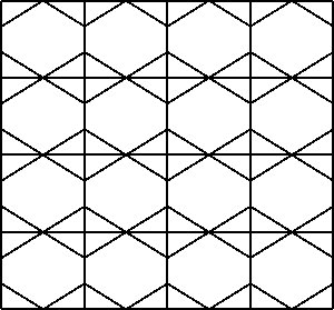
(a) Hexagonal

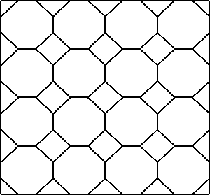
(b) Octagonal

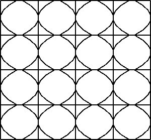
(c) Hexadecagonal

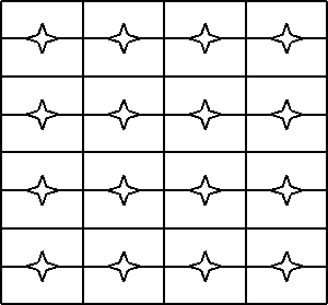
(d) Star Concave

Figure 1: Meshes

In each case we start from a mesh of $\#\mathcal{M}_{h}$ polygons then we refine it, obtaining meshes made by $4\#\mathcal{M}_{h}$, $16\#\mathcal{M}_{h}$ and $64\#\mathcal{M}_{h}$ polygons. The first and the third sequence start with $\#\mathcal{M}_{h}$ equal to $320$, the second and the fourth with $\#\mathcal{M}_{h}$ equal to $164$ and $192$ respectively.

6.2.2 Convergence results

For the four mesh sequences, we report the trend of the $\mathrm{H}^{1}$ and the $\mathrm{L}^{2}$ errors in Figure 2a and in Figure 2b, respectively, decreasing the maximum diameter of the polygons. In the legends, we report the computed convergence rates with respect to $h$, denoted by $\alpha$. We see that we get the expected values for all the meshes, as obtained in 57 and 65.

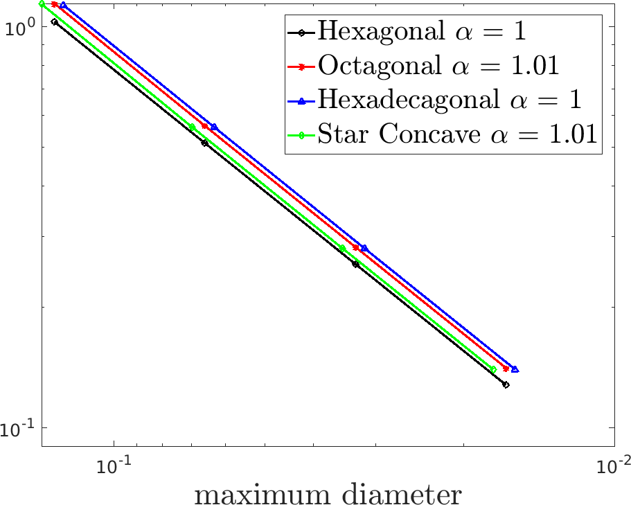
(a) $\mathrm{H}^{1}$ error

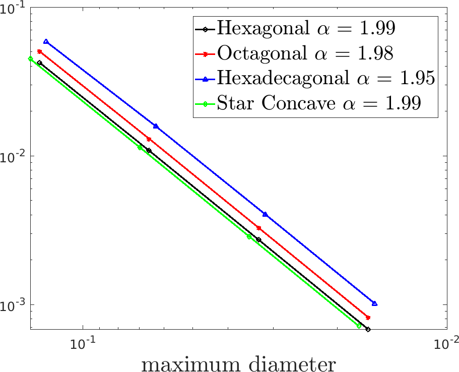
(b) $\mathrm{L}^{2}$ error

Figure 2: Logarithmic convergence plots

6.2.3 Convergence of diffusion-reaction discrete problem

(a) $\mathrm{H}^{1}$ error

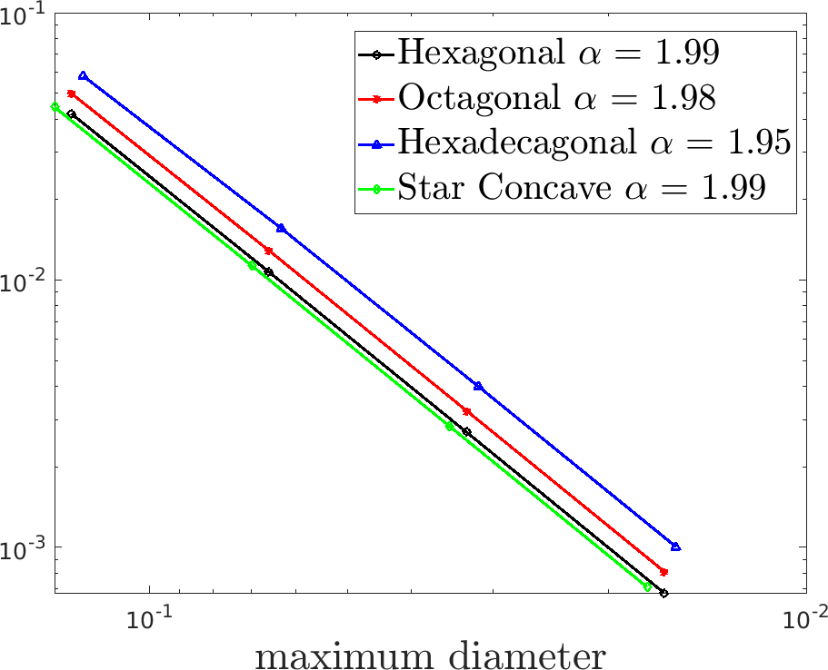
(b) $\mathrm{L}^{2}$ error

Figure 3: Logarithmic convergence plots for diffusion-reaction model

We finally report, in Figure 3, the $H^{1}$ and $L^{2}$ errors obtained for the four mesh sequences when solving 66 using the discrete formulation 67. We can see that the convergence rates $\alpha$ reported in the legends are optimal.

Appendix A Supplementary materials

A.1 Proof of Lemma 4

In order to show the proof, we have to present a preliminary result.

Lemma 9.

Let $\bar{q}\in\mathcal{R_{Q}}(E)$. Then $\exists C>0$, independent of $h_{E}$, such that

$$\sum_{i=1}^{N^{V}_{E}}\left\lvert{\bar{q}(x_{i})}\right\rvert\leq C\sqrt{\sum_{\tau\in\mathcal{T}_{E}}\left\lVert{\nabla\bar{q}}\right\rVert_{\mathrm{L}^{2}\!(\tau)}^{2}}\,.$$ (68)

Proof.

We notice that

$$\sum_{i=1}^{N^{V}_{E}}\left\lvert{\bar{q}(x_{i})}\right\rvert=\frac{1}{2}\sum_{\tau\in\mathcal{T}_{E}}\left(\left\lvert{\bar{q}(x_{\tau,1})}\right\rvert+\left\lvert{\bar{q}(x_{\tau,2})}\right\rvert\right)\,,$$ (69)

where $x_{\tau,1}$ and $x_{\tau,2}$ are the vertices of $\tau$ that are on $\partial E$. We have that

$${\bar{q}}_{|\tau}\in\tilde{\mathbb{P}}_{1}(\tau)=\left\{p\in\mathbb{P}_{1}\!\left(\tau\right)\colon p(x_{C})=0\right\}\,,$$

and

$$\left\lvert{\bar{q}(x_{\tau,1})}\right\rvert+\left\lvert{\bar{q}(x_{\tau,2})}\right\rvert=\left\lVert{\mathrm{dof}_{\tilde{\mathbb{P}}_{1}(\tau)}\left({\bar{q}}_{|\tau}\right)}\right\rVert_{l^{1}}\,,$$

having chosen the values at $x_{\tau,1}$ and $x_{\tau,2}$ as set of degrees of freedom on $\tilde{\mathbb{P}}_{1}(\tau)$ and denoting by $\mathrm{dof}_{\tilde{\mathbb{P}}_{1}(\tau)}\left(\cdot\right)$ the operator returning the vector of such values. Using the mapping 18 we get

$$\left\lVert{\mathrm{dof}_{\tilde{\mathbb{P}}_{1}(\tau)}\left({\bar{q}}_{|\tau}\right)}\right\rVert_{l^{1}}=\left\lVert{\mathrm{dof}_{\tilde{\mathbb{P}}_{1}(\hat{\tau})}\left({\hat{\bar{q}}}_{|\hat{\tau}}\right)}\right\rVert_{l^{1}}\,.$$

The right-hand side of the above equation is a norm on $\tilde{\mathbb{P}}_{1}(\hat{\tau})$, as well as $\left\lVert{\hat{\nabla}\hat{\bar{q}}}\right\rVert_{\mathrm{L}^{2}\!(\hat{\tau})}$. Then, by standard arguments about the equivalence of norms in finite dimensional spaces, we have

$$\left\lVert{\mathrm{dof}_{\tilde{\mathbb{P}}_{1}(\hat{\tau})}\left({\hat{\bar{q}}}_{|\hat{\tau}}\right)}\right\rVert_{l^{1}}\leq\frac{\sqrt{2}\max_{i=1,2}\left\lVert{\mathrm{dof}_{\tilde{\mathbb{P}}_{1}(\hat{\tau})}\left(\hat{\chi}_{i}\right)}\right\rVert_{l^{1}}}{\min_{\hat{w}\in\tilde{\mathbb{P}}_{1}(\hat{\tau})\colon\hat{w}(\hat{x}_{\hat{\tau},1})^{2}+\hat{w}(\hat{x}_{\hat{\tau},2})^{2}=1}\left\lVert{\hat{\nabla}\hat{w}}\right\rVert_{\mathrm{L}^{2}\!(\hat{\tau})}}\left\lVert{\hat{\nabla}\hat{\bar{q}}}\right\rVert_{\mathrm{L}^{2}\!(\hat{\tau})}\,,$$

where the $\hat{\chi}_{i}$ are Lagrangian in the degrees of freedom. Then, $\left\lVert{\mathrm{dof}_{\tilde{\mathbb{P}}_{1}(\hat{\tau})}\left(\hat{\chi}_{1}\right)}\right\rVert_{l^{1}}=\left\lVert{\mathrm{dof}_{\tilde{\mathbb{P}}_{1}(\hat{\tau})}\left(\hat{\chi}_{2}\right)}\right\rVert_{l^{1}}=1$ and

$$\left\lVert{\mathrm{dof}_{\tilde{\mathbb{P}}_{1}(\hat{\tau})}\left({\hat{\bar{q}}}_{|\hat{\tau}}\right)}\right\rVert_{l^{1}}\leq\frac{\sqrt{2}}{\min_{\hat{w}\in\tilde{\mathbb{P}}_{1}(\hat{\tau})\colon\hat{w}(\hat{x}_{\hat{\tau},1})^{2}+\hat{w}(\hat{x}_{\hat{\tau},2})^{2}=1}\left\lVert{\hat{\nabla}\hat{w}}\right\rVert_{\mathrm{L}^{2}\!(\hat{\tau})}}\left\lVert{\hat{\nabla}\hat{\bar{q}}}\right\rVert_{\mathrm{L}^{2}\!(\hat{\tau})}\,.$$

It can be proved by standard arguments that the constant in the above inequality is continuous with respect to $\hat{\tau}$, since it depends continuously on the deformation of the domain (see the proofs of [28, Lemma 4.9] and [11, Lemma 4.5]). It follows by compactness of the set of admissible reference elements, denoted by $\Sigma$, (Lemma 3) that there exists $M>0$ such that

$$M=\max_{\hat{\tau}\in\Sigma}\frac{\sqrt{2}}{\min_{\hat{w}\in\tilde{\mathbb{P}}_{1}(\hat{\tau})\colon\hat{w}(\hat{x}_{\hat{\tau},1})^{2}+\hat{w}(\hat{x}_{\hat{\tau},2})^{2}=1}\left\lVert{\hat{\nabla}\hat{w}}\right\rVert_{\mathrm{L}^{2}\!(\hat{\tau})}}\,,$$

and thus, starting again from 69 and applying the mapping 18, we get

$$\begin{split}\sum_{i=1}^{N^{V}_{E}}\left\lvert{\bar{q}(x_{i})}\right\rvert&=\frac{1}{2}\sum_{\tau\in\mathcal{T}_{E}}\left\lVert{\mathrm{dof}_{\tilde{\mathbb{P}}_{1}(\tau)}\left({\bar{q}}_{|\tau}\right)}\right\rVert_{l^{1}}=\frac{1}{2}\sum_{\hat{\tau}\in\mathcal{T}_{\hat{E}}}\left\lVert{\mathrm{dof}_{\tilde{\mathbb{P}}_{1}(\hat{\tau})}\left({\hat{\bar{q}}}_{|\hat{\tau}}\right)}\right\rVert_{l^{1}}\\ &\leq\frac{M}{2}\sum_{\hat{\tau}\in\mathcal{T}_{\hat{E}}}\left\lVert{\hat{\nabla}\hat{\bar{q}}}\right\rVert_{\mathrm{L}^{2}\!(\hat{\tau})}=\frac{M}{2}\sum_{\tau\in\mathcal{T}_{E}}\left\lVert{\nabla\bar{q}}\right\rVert_{\mathrm{L}^{2}\!(\tau)}\\ &\leq\frac{M\sqrt{N^{V}_{E}}}{2}\sqrt{\sum_{\tau\in\mathcal{T}_{E}}\left\lVert{\nabla\bar{q}}\right\rVert_{\mathrm{L}^{2}\!(\tau)}^{2}}\,,\end{split}$$

and we obtain 68 since $N^{V}_{E}$ is uniformly bounded by 4. ∎

Now, we can present the proof of Lemma 4.

Proof.

Let $\bar{q}\in\mathcal{R_{Q}}(E)$ and $\boldsymbol{v}\in V\left(E\right)$ be given. Starting from 26 and applying the triangular inequality, we have

$$\left\lvert{b(\bar{q},\boldsymbol{v})}\right\rvert\leq\left\lvert{\sum_{\tau\in\mathcal{T}_{E}}\limits\int_{\tau}\left[\nabla\bar{q}\,\boldsymbol{v}+\bar{q}\,\nabla\cdot\boldsymbol{v}\right]\,dx}\right\rvert+\left\lvert{\sum_{i=1}^{N^{V}_{E}}\limits\int_{e_{i}}\limits\gamma^{e_{i}}\!\left(\bar{q}\right)\left\llbracket{\boldsymbol{v}}\right\rrbracket_{e_{i}}\cdot\boldsymbol{n}^{e_{i}}ds}\right\rvert.$$ (70)

Let us consider separately the two terms involved in the inequality. The first part can be analysed applying the property,

$$\forall\bar{q}\in\mathcal{R_{Q}}(E),\quad\sum_{\tau\in\mathcal{T}_{E}}\left(\left\lVert{\bar{q}}\right\rVert_{\mathrm{L}^{2}\!(\tau)}+\left\lVert{\nabla\bar{q}}\right\rVert_{\left[\mathrm{L}^{2}\!\left(\tau\right)\right]^{2}}\right)\leq\sqrt{2N^{V}_{E}}\left\lVert{\bar{q}}\right\rVert_{\mathrm{H}^{1}_{\mathcal{T}}\!(E)}$$

and the mesh assumption 4, as follows

$$\left\lvert{\sum_{\tau\in\mathcal{T}_{E}}\limits\int_{\tau}\left[\nabla\bar{q}\,\boldsymbol{v}+\bar{q}\,\nabla\cdot\boldsymbol{v}\right]\,dx}\right\rvert \leq\sum_{\tau\in\mathcal{T}_{E}}\limits\left(\left\lVert{\nabla\bar{q}}\right\rVert_{\left[\mathrm{L}^{2}\!\left(\tau\right)\right]^{2}}\left\lVert{\boldsymbol{v}}\right\rVert_{\left[\mathrm{L}^{2}\!\left(\tau\right)\right]^{2}}+\left\lVert{\bar{q}}\right\rVert_{\mathrm{L}^{2}\!(\tau)}\left\lVert{\nabla\cdot\boldsymbol{v}}\right\rVert_{\mathrm{L}^{2}\!(\tau)}\right)$$

$$\leq C\sum_{\tau\in\mathcal{T}_{E}}\limits\left(\left\lVert{\boldsymbol{v}}\right\rVert_{\left[\mathrm{L}^{2}\!\left(\tau\right)\right]^{2}}+\left\lVert{\nabla\cdot\boldsymbol{v}}\right\rVert_{\mathrm{L}^{2}\!(\tau)}\right)$$

$$\quad\times\left(\left\lVert{\nabla\bar{q}}\right\rVert_{\left[\mathrm{L}^{2}\!\left(\tau\right)\right]^{2}}+\left\lVert{\bar{q}}\right\rVert_{\mathrm{L}^{2}\!(\tau)}\right)$$

$$\leq C\left\lVert{\bar{q}}\right\rVert_{\mathrm{H}^{1}_{\mathcal{T}}\!(E)}\sum_{\tau\in\mathcal{T}_{E}}\limits\left(\left\lVert{\boldsymbol{v}}\right\rVert_{\left[\mathrm{L}^{2}\!\left(\tau\right)\right]^{2}}+\left\lVert{\nabla\cdot\boldsymbol{v}}\right\rVert_{\mathrm{L}^{2}\!(\tau)}\right).$$

Moreover, let us consider the second term of 70, computing exactly the term $\left\lVert{\gamma^{e_{i}}\!\left(\bar{q}\right)}\right\rVert_{\mathrm{L}^{2}\!(e_{i})}$ and applying the properties $\forall\boldsymbol{v}\in V\left(E\right)$

$$\sum_{i=1}^{N^{V}_{E}}\limits\left\lVert{\left\llbracket{\boldsymbol{v}}\right\rrbracket_{e_{i}}}\right\rVert_{\mathrm{L}^{2}\!(e_{i})}\leq\sqrt{2N^{V}_{E}}\sqrt{\sum_{i=1}^{N^{V}_{E}}\limits\left\lVert{\left\llbracket{\boldsymbol{v}}\right\rrbracket_{e_{i}}}\right\rVert_{\mathrm{L}^{2}\!(e_{i})}^{2}}\,,$$

$$\left\lVert{\left\llbracket{\boldsymbol{v}}\right\rrbracket_{e_{i}}}\right\rVert_{\mathrm{L}^{2}\!(e_{i})}^{2}\leq h_{E}\left\lVert{\left\llbracket{\boldsymbol{v}}\right\rrbracket_{\mathcal{I}_{\mathcal{E}_{E}}}}\right\rVert_{\mathrm{L}^{\infty}\left({\mathcal{I}_{\mathcal{E}_{E}}}\right)}^{2},\;\forall e_{i}\in\mathcal{I}_{\mathcal{E}_{E}}\,,$$

we have

$$\left\lvert{\sum_{i=1}^{N^{V}_{E}}\limits\int_{e_{i}}\limits\gamma^{e_{i}}\!\left(\bar{q}\right)\left\llbracket{\boldsymbol{v}}\right\rrbracket_{e_{i}}\cdot\boldsymbol{n}^{e_{i}}ds}\right\rvert \leq\sum_{i=1}^{N^{V}_{E}}\limits\left\lVert{\gamma^{e_{i}}\!\left(\bar{q}\right)}\right\rVert_{\mathrm{L}^{2}\!(e_{i})}\left\lVert{\left\llbracket{\boldsymbol{v}}\right\rrbracket_{e_{i}}\cdot\boldsymbol{n}^{e_{i}}}\right\rVert_{\mathrm{L}^{2}\!(e_{i})}$$

$$\leq\sum_{i=1}^{N^{V}_{E}}\limits\frac{\sqrt{h_{e_{i}}}}{\sqrt{3}}\left\lvert{\bar{q}(x_{i})}\right\rvert\left\lVert{\left\llbracket{\boldsymbol{v}}\right\rrbracket_{e_{i}}}\right\rVert_{\left[\mathrm{L}^{2}\!\left(e_{i}\right)\right]^{2}}$$

$$\leq\frac{h_{E}}{\sqrt{3}}\left\lVert{\left\llbracket{\boldsymbol{v}}\right\rrbracket_{\mathcal{I}_{\mathcal{E}_{E}}}}\right\rVert_{\mathrm{L}^{\infty}\left({\mathcal{I}_{\mathcal{E}_{E}}}\right)}\sum_{i=1}^{N^{V}_{E}}\limits\left\lvert{\bar{q}(x_{i})}\right\rvert$$

$$\leq Ch_{E}\left\lVert{\left\llbracket{\boldsymbol{v}}\right\rrbracket_{\mathcal{I}_{\mathcal{E}_{E}}}}\right\rVert_{\mathrm{L}^{\infty}\left({\mathcal{I}_{\mathcal{E}_{E}}}\right)}\left\lVert{\bar{q}}\right\rVert_{\mathrm{H}^{1}_{\mathcal{T}}\!(E)}\,,$$

where we apply Lemma 9 in the last step. Finally, substituting into 70, we obtain

$$\left\lvert{b(\bar{q},\boldsymbol{v})}\right\rvert \leq C\left\lVert{\bar{q}}\right\rVert_{\mathrm{H}^{1}_{\mathcal{T}}\!(E)}\left(\sum_{\tau\in\mathcal{T}_{E}}\limits\left(\left\lVert{\boldsymbol{v}}\right\rVert_{\left[\mathrm{L}^{2}\!\left(\tau\right)\right]^{2}}+\left\lVert{\nabla\cdot\boldsymbol{v}}\right\rVert_{\mathrm{L}^{2}\!(\tau)}\right)+h_{E}\left\lVert{\left\llbracket{\boldsymbol{v}}\right\rrbracket_{\mathcal{I}_{\mathcal{E}_{E}}}}\right\rVert_{\mathrm{L}^{\infty}\left({\mathcal{I}_{\mathcal{E}_{E}}}\right)}\right)$$

$$\leq C\left\lVert{\bar{q}}\right\rVert_{\mathrm{H}^{1}_{\mathcal{T}}\!(E)}\left\lVert{\boldsymbol{v}}\right\rVert_{V\left(E\right)}\,.$$

∎

A.2 Proof of Theorem 5

Proof.

Let us define the auxiliary problem: let $\Psi\in\mathrm{H}^{2}\!(\Omega)\cap\mathrm{H}^{1}_{0}\!(\Omega)$ the solution of ${a}\left(V,\Psi\right)=\left(U-u,V\right)_{\Omega}$ $\forall V\in\mathrm{H}^{1}_{0}\!(\Omega)$. From the definition of $\Psi$, we get:

$$\exists C>0:\quad\left\lvert{\Psi}\right\rvert_{2} \leq C\left\lVert{U-u}\right\rVert_{\mathrm{L}^{2}\!(\Omega)},$$ (71)

$$\exists C>0:\quad\left\lVert{\Psi}\right\rVert_{\mathrm{H}^{1}_{0}\!(\Omega)} \leq C\left\lVert{U-u}\right\rVert_{\mathrm{L}^{2}\!(\Omega)}.$$ (72)

Let us denote by $\Psi_{I}$ the interpolant of $\Psi$ according to Lemma 7. Applying the auxiliary problem, the discrete problem 11 and the definition of the bilinear form $a$ 2, we have

$$\left\lVert{U-u}\right\rVert_{\mathrm{L}^{2}\!(\Omega)}^{2} =\left(U-u,U-u\right)_{\Omega}={a}\left(U-u,\Psi\right)$$

$$={a}\left(U,\Psi-\Psi_{I}\right)+{a}\left(U,\Psi_{I}\right)-{a}\left(u,\Psi\right)$$

$$={a}\left(U,\Psi-\Psi_{I}\right)+\left(f,\Psi_{I}\right)_{\Omega}-{a}\left(u,\Psi\right)$$

$$\begin{gathered}={a}\left(U,\Psi-\Psi_{I}\right)+\left(f,\Psi_{I}\right)_{\Omega}-\left(\sum_{E\in\mathcal{M}_{h}}\left(f,\Pi^{0}_{0,E}\Psi_{I}\right)_{E}\right)\\ +{a}_{h}\left(u,\Psi_{I}\right)-{a}\left(u,\Psi\right)+{a}\left(u,\Psi_{I}\right)-{a}\left(u,\Psi_{I}\right)\end{gathered}$$ (75)

$$\begin{gathered}={a}\left(U-u,\Psi-\Psi_{I}\right)+\left(\sum_{E\in\mathcal{M}_{h}}\left(f,\Psi_{I}-\Pi^{0}_{0,E}\Psi_{I}\right)_{E}\right)\\ +{a}_{h}\left(u,\Psi_{I}\right)-{a}\left(u,\Psi_{I}\right).\end{gathered}$$ (78)

Let us consider the terms of the previous relation separately. First, applying the Cauchy-Schwarz inequality, 54, 56 and 71, we have, for the first term,

$${a}\left(U-u,\Psi-\Psi_{I}\right) \leq\left\lVert{U-u}\right\rVert_{\mathrm{H}^{1}_{0}\!(\Omega)}\left\lVert{\Psi-\Psi_{I}}\right\rVert_{\mathrm{H}^{1}_{0}\!(\Omega)}$$

$$\leq Ch\left\lVert{U-u}\right\rVert_{\mathrm{H}^{1}_{0}\!(\Omega)}\left\lvert{\Psi}\right\rvert_{2}\leq Ch\left\lVert{U-u}\right\rVert_{\mathrm{H}^{1}_{0}\!(\Omega)}\left\lVert{U-u}\right\rVert_{\mathrm{L}^{2}\!(\Omega)},$$ (79)

and, for the second one,

$$\sum_{E\in\mathcal{M}_{h}}\left(f,\Psi_{I}-\Pi^{0}_{0,E}\Psi_{I}\right)_{E} =\sum_{E\in\mathcal{M}_{h}}\left(f-\Pi^{0}_{0,E}f,\Psi_{I}-\Pi^{0}_{0,E}\Psi_{I}\right)_{E}$$

$$\leq\sum_{E\in\mathcal{M}_{h}}\left\lVert{f-\Pi^{0}_{0,E}f}\right\rVert_{\mathrm{L}^{2}\!(E)}\left\lVert{\Psi_{I}-\Pi^{0}_{0,E}\Psi_{I}}\right\rVert_{\mathrm{L}^{2}\!(E)}$$

$$\leq Ch\left\lvert{f}\right\rvert_{\mathrm{H}^{1}\!(\Omega)}\sum_{E\in\mathcal{M}_{h}}\left\lVert{\Psi_{I}-\Pi^{0}_{0,E}\Psi_{I}}\right\rVert_{\mathrm{L}^{2}\!(E)}.$$ (80)

Applying the property

$$\forall E\in\mathcal{M}_{h},\;\;\left\lVert{\Psi_{I}-\Pi^{0}_{0,E}\Psi_{I}}\right\rVert_{\mathrm{L}^{2}\!(E)}\leq\left\lVert{\Psi_{I}-\Pi^{0}_{0,E}\Psi}\right\rVert_{\mathrm{L}^{2}\!(E)},$$

54 and 56 to 80, we obtain

$$\sum_{E\in\mathcal{M}_{h}}\left(f,\Psi_{I}-\Pi^{0}_{0,E}\Psi_{I}\right)_{E} \leq Ch\left\lvert{f}\right\rvert_{\mathrm{H}^{1}\!(\Omega)}\sum_{E\in\mathcal{M}_{h}}\left\lVert{\Psi_{I}-\Pi^{0}_{0,E}\Psi}\right\rVert_{\mathrm{L}^{2}\!(E)}$$

$$\leq Ch\left\lvert{f}\right\rvert_{\mathrm{H}^{1}\!(\Omega)}\sum_{E\in\mathcal{M}_{h}}\left(\left\lVert{\Psi_{I}-\Psi}\right\rVert_{\mathrm{L}^{2}\!(E)}+\left\lVert{\Psi-\Pi^{0}_{0,E}\Psi}\right\rVert_{\mathrm{L}^{2}\!(E)}\right)$$

$$\leq Ch\left\lvert{f}\right\rvert_{\mathrm{H}^{1}\!(\Omega)}\left(h^{2}\left\lvert{\Psi}\right\rvert_{2}+h\left\lVert{\Psi}\right\rVert_{\mathrm{H}^{1}_{0}\!(\Omega)}\right).$$ (81)

We can omit higher order terms and apply 72, obtaining

$$\sum_{E\in\mathcal{M}_{h}}\left(f,\Psi_{I}-\Pi^{0}_{0,E}\Psi_{I}\right)_{E}\leq Ch^{2}\left\lvert{f}\right\rvert_{\mathrm{H}^{1}\!(\Omega)}\left\lVert{U-u}\right\rVert_{\mathrm{L}^{2}\!(\Omega)}.$$ (82)

Finally, we have to bound ${a}_{h}\left(u,\Psi_{I}\right)-{a}\left(u,\Psi_{I}\right)$. Then, applying the orthogonality property of $\Pi^{0}_{l,E}$, adding and subtracting terms, we have

$${a}_{h}\left(u,\Psi_{I}\right)-{a}\left(u,\Psi_{I}\right) =\sum_{E\in\mathcal{M}_{h}}\left(\Pi^{0}_{l,E}\nabla u,\nabla\Psi_{I}\right)_{E}-\left(\nabla u,\nabla\Psi_{I}\right)_{E}$$

$$=\sum_{E\in\mathcal{M}_{h}}\left(\Pi^{0}_{l,E}\nabla u-\nabla u,\nabla\Psi_{I}-\Pi^{0}_{0,E}\nabla\Psi_{I}\right)_{E}$$

$$\begin{gathered}=\sum_{E\in\mathcal{M}_{h}}\left(\Pi^{0}_{l,E}\nabla u-\Pi^{0}_{l,E}\nabla U,\nabla\Psi_{I}-\Pi^{0}_{0,E}\nabla\Psi_{I}\right)_{E}\\ +\left(\Pi^{0}_{l,E}\nabla U-\nabla U,\nabla\Psi_{I}-\Pi^{0}_{0,E}\nabla\Psi_{I}\right)_{E}\\ +\left(\nabla U-\nabla u,\nabla\Psi_{I}-\Pi^{0}_{0,E}\nabla\Psi_{I}\right)_{E}.\end{gathered}$$ (86)

Notice that, applying 54 and 55, we have the property $\forall E\in\mathcal{M}_{h}$ :

$$\left\lVert{\nabla\Psi_{I}-\Pi^{0}_{0,E}\nabla\Psi_{I}}\right\rVert_{\mathrm{L}^{2}\!(E)}\leq\left\lVert{\nabla\Psi_{I}-\Pi^{0}_{0,E}\nabla\Psi}\right\rVert_{\mathrm{L}^{2}\!(E)}\leq Ch\left\lvert{\Psi}\right\rvert_{2,E}.$$

Therefore, applying the continuity of the projection operator and 71, the first and the last term of 86 can be bounded as

$$\begin{gathered}\sum_{E\in\mathcal{M}_{h}}\left(\Pi^{0}_{l,E}\nabla u-\Pi^{0}_{l,E}\nabla U,\nabla\Psi_{I}-\Pi^{0}_{0,E}\nabla\Psi_{I}\right)_{E}+\left(\nabla U-\nabla u,\nabla\Psi_{I}-\Pi^{0}_{0,E}\nabla\Psi_{I}\right)_{E}\\ \leq Ch\left\lVert{U-u}\right\rVert_{\mathrm{H}^{1}_{0}\!(\Omega)}\left\lVert{U-u}\right\rVert_{\mathrm{L}^{2}\!(\Omega)}.\end{gathered}$$ (87)

Similarly, the second term is bounded as

$$\sum_{E\in\mathcal{M}_{h}}\left(\Pi^{0}_{l,E}\nabla U-\nabla U,\nabla\Psi_{I}-\Pi^{0}_{0,E}\nabla\Psi_{I}\right)_{E}\leq Ch^{2}\left\lvert{U}\right\rvert_{2}\left\lVert{U-u}\right\rVert_{\mathrm{L}^{2}\!(\Omega)}.$$ (88)

Finally, applying 79,82,87 and 88 to 78 and simplifying, we obtain

$$\left\lVert{U-u}\right\rVert_{\mathrm{L}^{2}\!(\Omega)}\leq C\left(h\left\lVert{U-u}\right\rVert_{\mathrm{H}^{1}_{0}\!(\Omega)}+h^{2}\left\lvert{f}\right\rvert_{\mathrm{H}^{1}\!(\Omega)}+h^{2}\left\lvert{U}\right\rvert_{2}\right).$$

Applying the $\mathrm{H}^{1}$-estimate (Theorem 4) we obtain the relation 65. ∎

References

• [1] B. Ahmad, A. Alsaedi, F. Brezzi, L. D. Marini, and A. Russo. Equivalent projectors for virtual element methods. Computers & Mathematics with Applications, 66:376–391, September 2013.
• [2] P. F. Antonietti, S. Berrone, A. Borio, A. D’Auria, M. Verani, and S. Weisser. Anisotropic a posteriori error estimate for the virtual element method. IMA Journal of Numerical Analysis, 02 2021.
• [3] P. F. Antonietti, L. Mascotto, and M. Verani. A multigrid algorithm for the $p$-version of the virtual element method. ESAIM: Mathematical Modelling and Numerical Analysis, 52:337–364, 03 2017.
• [4] I. Babuška, E. G. Podnos, and G. J. Rodin. New fictitious domain methods: formulation and analysis. Mathematical Models and Methods in Applied Sciences, 15(10):1575–1594, 2005.
• [5] L. Beirão da Veiga, F. Brezzi, A. Cangiani, G. Manzini, L. D. Marini, and A. Russo. Basic principles of virtual element methods. Mathematical Models and Methods in Applied Sciences, 23(01):199–214, 2013.
• [6] L. Beirão da Veiga, F. Brezzi, L. D. Marini, and A. Russo. Virtual element methods for general second order elliptic problems on polygonal meshes. Mathematical Models and Methods in Applied Sciences, 26(04):729–750, 2015.
• [7] L. Beirão da Veiga, F. Brezzi, L. D. Marini, and A. Russo. Mixed virtual element methods for general second order elliptic problems on polygonal meshes. ESAIM: Mathematical Modelling and Numerical Analysis, 50(3):727–747, 2016.
• [8] L. Beirão da Veiga, K. Lipnikov, and G. Manzini. The mimetic finite difference method for elliptic problems. Ms&A Modeling, simulation and applications 11. Springer, Cham, 2014.
• [9] L. Beirão da Veiga, C. Lovadina, and D. Mora. A virtual element method for elastic and inelastic problems on polytope meshes. Computer Methods in Applied Mechanics and Engineering, 295:327–346, 2015.
• [10] L. Beirão da Veiga, C. Lovadina, and A. Russo. Stability analysis for the virtual element method. Mathematical Models and Methods in Applied Sciences, 27(13):2557–2594, 2017.
• [11] L. Beirão da Veiga and G. Manzini. Residual a posteriori error estimation for the virtual element method for elliptic problems. ESAIM: M2AN, 49(2):577–599, 2015.
• [12] M. F. Benedetto, S. Berrone, and A. Borio. The Virtual Element Method for underground flow simulations in fractured media. In Advances in Discretization Methods, volume 12 of SEMA SIMAI Springer Series, pages 167–186. Springer International Publishing, Switzerland, 2016.
• [13] M. F. Benedetto, S. Berrone, A. Borio, S. Pieraccini, and S. Scialò. A hybrid mortar virtual element method for discrete fracture network simulations. J. Comput. Phys., 306:148–166, 2016.
• [14] M. F. Benedetto, S. Berrone, A. Borio, S. Pieraccini, and S. Scialò. Order preserving SUPG stabilization for the virtual element formulation of advection-diffusion problems. Comput. Methods Appl. Mech. Engrg., 311:18 – 40, 2016.
• [15] M. F. Benedetto, S. Berrone, and S. Scialò. A globally conforming method for solving flow in discrete fracture networks using the virtual element method. Finite Elem. Anal. Des., 109:23–36, 2016.
• [16] S. Berrone and A. Borio. A residual a posteriori error estimate for the virtual element method. Mathematical Models and Methods in Applied Sciences, 27(08):1423–1458, 2017.
• [17] S. Berrone, A. Borio, and G. Manzini. SUPG stabilization for the nonconforming virtual element method for advection–diffusion–reaction equations. Computer Methods in Applied Mechanics and Engineering, 340:500 – 529, 2018.
• [18] S. Berrone, A. Borio, and F. Marcon. Comparison of standard and stabilization free virtual elements on anisotropic elliptic problems. Applied Mathematics Letters, 129:107971, 2022.
• [19] S. Berrone, S. Pieraccini, and S. Scialò. On simulations of discrete fracture network flows with an optimization-based extended finite element method. SIAM J. Sci. Comput., 35(2):A908–A935, 2013.
• [20] S. Berrone, S. Pieraccini, and S. Scialò. A PDE-constrained optimization formulation for discrete fracture network flows. SIAM J. Sci. Comput., 35(2):B487–B510, 2013.
• [21] S. Berrone, S. Pieraccini, and S. Scialò. An optimization approach for large scale simulations of discrete fracture network flows. J. Comput. Phys., 256:838–853, 2014.
• [22] D. Boffi, F. Brezzi, and M. Fortin. Approximation of Saddle Point Problems, chapter 5, pages 265–335. Springer Berlin Heidelberg, Berlin, Heidelberg, 2013.
• [23] S. C. Brenner and L. Sung. Virtual element methods on meshes with small edges or faces. Mathematical Models and Methods in Applied Sciences, 28(07):1291–1336, 2018.
• [24] F. Brezzi, K. Lipnikov, and V. Simoncini. A family of mimetic finite difference methods on polygonal and polyhedral meshes. Mathematical Models and Methods in Applied Sciences, 15(10):1533–1551, 2005.
• [25] F. Brezzi and L. D. Marini. Virtual element methods for plate bending problems. Computer Methods in Applied Mechanics and Engineering, 253:455–462, 2013.
• [26] E. Burman, S. Claus, P. Hansbo, M. G. Larson, and A. Massing. CutFEM: Discretizing geometry and partial differential equations. International Journal for Numerical Methods in Engineering, 104(7):472–501, 2015.
• [27] A. Cangiani, E. H. Georgoulis, T. Pryer, and O. J. Sutton. A posteriori error estimates for the virtual element method. Numerische Mathematik, 137(4):857–893, Dec 2017.
• [28] A. Cangiani, G. Manzini, and O. J. Sutton. Conforming and nonconforming virtual element methods for elliptic problems. IMA Journal of Numerical Analysis, 37(3):1317–1354, 08 2016.
• [29] L. Desiderio, S. Falletta, and L. Scuderi. A virtual element method coupled with a boundary integral non reflecting condition for 2d exterior helmholtz problems. Computers & Mathematics with Applications, 84:296–313, 2021.
• [30] D. A. Di Pietro and A. Ern. Mathematical Aspects of Discontinuous Galerkin Methods. Springer Berlin Heidelberg, Berlin, Heidelberg, 2012.
• [31] D. A. Di Pietro and A. Ern. A hybrid high-order locking-free method for linear elasticity on general meshes. Computer Methods in Applied Mechanics and Engineering, 283:1–21, 2015.
• [32] D. A. Di Pietro and A. Ern. Hybrid high-order methods for variable-diffusion problems on general meshes. Comptes Rendus Mathematique, 353(1):31–34, 2015.
• [33] D. A. Di Pietro, A. Ern, and S. Lemaire. An arbitrary-order and compact-stencil discretization of diffusion on general meshes based on local reconstruction operators. Computational Methods in Applied Mathematics, 14(4):461–472, 2014.
• [34] J. Droniou, R. Eymard, T. Gallou et, C. Guichard, and R. Herbin. The Gradient Discretisation Method. Mathématiques et Applications. Springer, Cham, 2018.
• [35] J. Droniou, R. Eymard, T. Gallou et, and R. Herbin. Gradient Schemes: a generic framework for the discretisation of linear, nonlinear and nonlocal elliptic and parabolic equations. Mathematical Models and Methods in Applied Sciences, 23(13):2395–2432, 2013.
• [36] R. Glowinski, T.-W. Pan, and J. Periaux. A fictitious domain method for Dirichlet problem and applications. Computer Methods in Applied Mechanics and Engineering, 111(3):283–303, 1994.
• [37] J. S Hesthaven and T. Warburton. Nodal Discontinuous Galerkin methods: algorithms, analysis, and applications. Texts in applied mathematics 54. Springer Science & Business Media, New York, 2008.
• [38] B. Hudobivnik, F. Aldakheel, and P. Wriggers. A low order 3D virtual element formulation for finite elasto–plastic deformations. Computational Mechanics, 63:253–269, 02 2019.
• [39] N. Moës, J. Dolbow, and T. Belytschko. A finite element method for crack growth without remeshing. International Journal for Numerical Methods in Engineering, 46(1):131–150, 1999.
• [40] C. S. Peskin. The immersed boundary method. Acta Numerica, 11:479–517, 2002.
• [41] B. Rivière. Discontinuous Galerkin Methods for Solving Elliptic and Parabolic Equations. Society for Industrial and Applied Mathematics, 2008.
• [42] T. Strouboulis, I. Babuška, and K. Copps. The design and analysis of the Generalized Finite Element Method. Computer Methods in Applied Mechanics and Engineering, 181(1):43–69, 2000.
• [43] T. Strouboulis, K. Copps, and I. Babuška. The generalized finite element method: an example of its implementation and illustration of its performance. International Journal for Numerical Methods in Engineering, 47(8):1401–1417, 2000.
• [44] T. Strouboulis, K. Copps, and I. Babuška. The generalized finite element method. Computer Methods in Applied Mechanics and Engineering, 190(32):4081–4193, 2001.
• [45] N. Sukumar and A. Tabarraei. Conforming polygonal finite elements. International Journal for Numerical Methods in Engineering, 61(12):2045–2066, 2004.
• [46] V. Tishkin, A. A. Samarskii, A. P. Favorskii, and M. Shashkov. Operational finite-difference schemes. Differential Equations, 17:854–862, 07 1981.
• [47] G. Vacca. Virtual element methods for hyperbolic problems on polygonal meshes. Computers & Mathematics with Applications, 74(5):882 – 898, 2017. SI: SDS2016 – Methods for PDEs.
• [48] G. Vacca and L. Beirão da Veiga. Virtual element methods for parabolic problems on polygonal meshes. Numerical Methods for Partial Differential Equations, 31(6):2110–2134, 2015.