Bilinear optimal stabilization of a non-homogeneous Fokker-Planck equation

Abstract

In this work, we study the bilinear optimal stabilization of a non-homogeneous Fokker-Planck equation. We first study the problem of optimal control in a finite-time interval and then focus on the case of the infinite time horizon. We further show that the obtained optimal control guarantees the strong stability of the system at hand. An illustrating numerical example is given.

I Introduction

In this paper we consider the following non-homogeneous bilinear system:

$$\begin{cases}\dot{y}(t,x)=\Delta y(t,x)+\sum_{i=1}^{N}u_{i}(t)\left(\frac{\partial y}{\partial x_{i}}(t,x)+b_{i}\right),(t,x)\in(0,T)\times\Omega\\ y(t,x)=0,\,\ \ \ \ \ \ \ \ \ \ \ \ \ \ \ \ \ \ \ \ \ \ \ \ \ \ \ \ \ \ \ \ \ \ \ \ \ \ \ \ \ \ \ \ \ \ \ (t,x)\in(0,T)\times\partial\Omega\\ y(0,x)=y_{0}\in L^{2}(\Omega),\ \ \ \ \ \ \ \ \ \ \ \ \ \ \ \ \ \ \ \ \ \ \ \ \ \ \ \ \ \ \ \ \ \ \ \ \ \ \ \ \ \ \ \ \ \ \ \ \ \ x\in\Omega\end{cases}$$ (1)

where $0<T\leq+\infty$, $\Omega$ is an open and bounded domain of $\mathbb{R}^{N}$, $N\in\{1,2,3\}$ and $b_{i}\in H_{0}^{2}(\Omega):=H_{0}^{1}(\Omega)\cap H^{2}(\Omega)$. Here, $u_{i}(t)$ design the controls and $y(t)$ the corresponding mild solution of the system (1).

In term of applications, equation like (1) may for instance describe the situation where some physical quantities (particles, energy,…) are transferred inside a system due to diffusion and convection processes, and the control can be seen as the velocity field that the quantity is moving with. For our special case, system (1) describes a deterministic Fokker–Planck equation for the time-dependent probability density ${P\left(A,t\right)}$ of a stochastic variable $A$ of the Langevin equation, which enables us to study many types of fluctuations in physical and biological systems (see e.g. [19]).

The goal of this paper is to study the problem of stability by an optimal control in the infinite time-horizon for the non-homogeneous bilinear system (1). The main difficulty in solving a quadratic optimal control for general bilinear systems is the non-convexity of the cost function. In the case of a bounded control operator, the question of bilinear optimal control problem has been widely studied in the literature (see [6, 11, 15, 20, 27, 28]). However, the modeling may give rise to the unboundedness aspect of the operator of control of the obtained bilinear model (see [1, 3, 7, 14, 16]), which is the case of equation (1) where the control is acting in the coefficient of the divergence term. In [1], the authors have considered the homogeneous version of the system (1) (i.e. $b_{i}=0,\;i=1,..,N$), for which they characterized the optimal control for a finite time horizon. Moreover, the author in [3, 14] has studied the same problem in the presence of a time and state-dependent perturbation for finite time horizon.

The paper is organized as follows: In Section II we give a preliminary. In Section III, we first solve the optimal control problem in a finite time-horizon for the system (1), and then proceed to the case of infinite time horizon in which context we give a stabilization result by optimal control. Finally, in Section 4, we present a numerical example.

II Setting of the problem and some a priori estimates

Let us consider the following spaces: $H=L^{2}(\Omega),\;V=H_{0}^{1}(\Omega),$ $V^{*}=H^{-1}(\Omega)$ and $U=L^{2}(0,T;\mathbb{R}^{N})$, and let us introduce the following operators :

• $A:V\rightarrow V^{*},\ y\mapsto\Delta y$ which is a linear continuous operator,

• the linear continuous operator $B:V\rightarrow V^{*}$, is defined by $By=1_{\Omega}.\nabla y=\sum_{i=1}^{N},\frac{\partial y}{\partial x_{i}}$, here $1_{\Omega}$ is the vector $(1,\cdots,1)$.

For all $u:=(u_{i})_{1\leq i\leq N}\in U$ and $y\in V$, we have

$$u.(By+b):=u.(\nabla y+b)=\sum_{i=1}^{N}y_{i}\,\left(\frac{\partial y}{\partial x_{i}}+b_{i}\right)\cdot$$

Thus the system (1) can be rewritten in the form

$$\begin{cases}\dot{y}(t)=Ay(t)+u(t).(By(t)+b)\\ y(0)=y_{0}\in H.\end{cases}$$ (2)

The quadratic cost function $J$ to be minimized is defined by

$$J(u)=\int_{0}^{T}\|y(t)\|_{H}^{2}dt+\frac{r}{2}\int_{0}^{T}\|u(t)\|_{\mathbb{R}^{N}}^{2}dt,$$ (3)

where $r>0$, $u\in U$ and $y(t)$ is the respective solution to system (2) .

Then, the optimal control problem may be stated as follows

$$\left\{\begin{array}[]{ll}\min J(u)\\ u\in U\\ \end{array}\right.$$ (4)

For the wellposedness of the system (2), let us consider the following system

$$\begin{cases}\dot{y}(t)=Ay(t)+u(t).By(t)+f(t)\\ y(0)=y_{0}\end{cases}$$ (5)

where $f\in L^{2}(0,T;V^{*})$, and let us introduce the following functional space

$$W(0,T)=\{\phi\in L^{2}(0,T,V)\ \ /\ \ \dot{\phi}\in L^{2}(0,T;V^{*})\}\cdot$$

Now, we recall the following existence result with some a priory estimates (see [1, 3, 14]).

Lemma 1

For all $u\in U$, there exists a unique solution $y$ of the system (5), which is such that

$$y\in W(0,T)\cap L^{\infty}(0,T;H)\cdot$$

Moreover, the following estimates hold

$$\|y\|_{L^{2}(0,T;V)}\leq\frac{1}{\sqrt{2}}\|y_{0}\|_{H}+\|f\|_{L^{2}(0,T;V^{*})}$$ (6)

$$\|y\|_{L^{\infty}(0,T;H)}\leq\|y_{0}\|_{H}+\sqrt{2}\|f\|_{L^{2}(0,T;V^{*})}$$ (7)

$$\|\dot{y}\|_{L^{(}0,T;V^{*})}\leq \left(\frac{1}{\sqrt{2}}\|y_{0}\|_{H}+\|f\|_{L^{2}(0,T;V^{*})}\right)\left(\alpha+\sqrt{2}\|u\|_{U}\right)$$ (8)

$$\ +\|f\|_{L^{2}(0,T;V^{*})}$$

where $\alpha$ is such that $\|Az\|_{V^{*}}\leq\alpha\|z\|_{V}$, for all $z\in V$.

III Characterization of the optimal control

III-A Existence of an optimal control

Theorem 2

For any $y_{0}\in H$, the problem (4) has at least one solution.

Proof 1

Since the set $\{J(u)/u\in U\}$ is not empty and is bounded from below, it admits a lower bound $J^{*}$.
Let $(u_{n})_{n\in\mathbb{N}}$ be a minimizing sequence such that $J(u_{n})\rightarrow J^{*}$.
Then the sequence $(u_{n})$ is bounded, so it admits a sub-sequence denoted by $(u_{n})$ as well, which weakly converges to $u^{*}\in U$.
Let $(y_{n})$ be the sequence of solutions of (2) corresponding to $(u_{n})$. According to Lemma 1, the sequences $\begin{aligned} \|y_{n}(0)\|_{H},\|y_{n}\|_{L^{2}(0,T;V)},\ \|y_{n}\|_{L^{\infty}(0,T;V)},\ \|\dot{y}_{n}\|_{L^{2}(0,T;V^{*})},\end{aligned}$ $\begin{aligned} \|Ay_{n}\|_{L^{2}(0,T;V^{*})}\end{aligned}$ and $\|u_{n}.(By_{n}+b)\|_{L^{2}(0,T;V^{*})}$ are bounded, so $(y_{n})$ admits a sub-sequence, also denoted by $(y_{n})$, such that

$$y_{n}\rightharpoonup y^{*}\ weakly\ in\ L^{2}(0,T;V),$$

$$y_{n}\rightharpoonup y^{*}\ weakly*\ \ in\ L^{\infty}(0,T;H),$$

$$\dot{y}_{n}\rightharpoonup\dot{y}^{*}\ weakly\ in\ L^{2}(0,T;V^{*}).$$

In addition to this, the linear operator

$$\mathbb{A}:L^{2}(0,T;V)\rightarrow L^{2}(0,T;V^{*})$$

$$y\mapsto\mathbb{A}y$$

is continuous, from which it follows that

$$\mathbb{A}y_{n}\rightharpoonup\mathbb{A}y^{*}\ weakly\ in\ L^{2}(0,T;V^{*})\cdot$$

Then since the embedding $W(0,T)\rightarrow L^{2}(0,T;H)$ is compact, $(y_{n})$ admits a sub-sequence, still denoted by $(y_{n})$, for which we have

$$y_{n}\rightarrow y^{*}\ strongly\ in\ L^{2}(0,T;H).$$ (9)

Taking into account that the operator $\mathbb{B}:L^{2}(0,T;H)\rightarrow L^{2}(0,T;V^{*})$ is linear and continuous, we deduce that

$$u_{n}.(\mathbb{B}y_{n}+b)\rightharpoonup u^{*}.(\mathbb{B}y^{*}+b)\ \ weakly\ in\ L^{2}(0,T;V^{*}).$$

Now, by taking the limit we deduce that

$$\begin{cases}\dot{y^{*}}(t)=Ay^{*}(t)+u^{*}(t).(By^{*}(t)+b)\\ y^{*}(0)=y_{0}\end{cases}$$

In other words, $y^{*}$ is the solution of the system (2) corresponding to control $u=u^{*}$.
Using that the norm $\|\cdot\|_{L^{2}(H)}$ is lower semi-continuous, it follows from the strong convergence of the sequence $y_{n}$ to $y^{*}$ in $L^{2}(0,T;H)$ that

$$\int_{0}^{T}\|y^{*}(t)\|_{H}^{2}dt\leq\liminf_{n\rightarrow+\infty}\int_{0}^{T}\|y_{n}(t)\|_{H}^{2}dt.$$ (10)

Since $R:u\mapsto\int_{0}^{T}\|u(t)\|_{U}^{2}dt$ is convex and lower semi-continuous with respect to the weak topology, we have (see Corollary III.8 of [13])

$$R(u^{*})\leq\liminf_{n\rightarrow+\infty}R(u_{n})\cdot$$ (11)

Combining the formulas (10) and (11) we deduce that

$$J(u^{*}) =\int_{0}^{T}\|y^{*}(t)\|_{H}^{2}dt+\frac{r}{2}\int_{0}^{T}\|u^{*}(t)\|_{\mathbb{R}^{N}}^{2}dt$$

$$\leq\liminf_{n\rightarrow+\infty}\int_{0}^{T}\|y_{n}(t)\|_{H}^{2}dt+\frac{r}{2}\liminf_{n\rightarrow+\infty}\int_{0}^{T}\|u_{n}(t)\|_{\mathbb{R}^{N}}^{2}dt$$

$$\leq\liminf_{n\rightarrow+\infty}J(u_{n})$$

$$\leq J^{*}\cdot$$

We conclude that $J(u^{*})=J^{*}$, and so $u^{*}$ is a solution of the problem (4).

III-B Expression of the optimal control for finite time-horizon

In this subsection, we will provide informations about the optimal control.

Theorem 3

For all $T>0$, the problem (4) admits a solution $u^{*}$ which is given by:

$$u_{i}^{*}(t)=-\dfrac{1}{r}\langle\phi(t),\frac{\partial y^{*}(t)}{\partial x_{i}}+b_{i}\rangle_{V^{*},V},\,\forall\,i=1,...,N,$$

where $y^{*}$ is the solution of the system (2) corresponding to $u^{*}$ and $\phi$ is the solution of the following adjoint system

$$\left\{\begin{array}[]{ll}\dot{\phi}(t)=-A\phi(t)+u^{*}(t).B\phi(t)-2y^{*}(t)\\ \phi(T)=0\end{array}\right.$$ (12)

Proof 2

First, let us show that the mapping

$$U\rightarrow C(0,T;H)$$

$$u\mapsto y_{u}$$

is Fréchet differentiable and that its derivative $z_{h}$ at $u\in U$, for a given $h\in U$, is the unique solution of the following system

$$\begin{cases}\dot{z_{h}}(t)=Az_{h}(t)+u(t).Bz_{h}(t)+h(t).(By_{u}(t)+b)\\ z_{h}(0)=0\end{cases}$$ (13)

Let $u\in U$ and let $y_{u}$ be the corresponding solution of the system (2). We claim that the linear mapping $h\mapsto z_{h}$ is continuous. Indeed, using the estimate (7) for the system (13), we can find some $M>0$ such that

$$\|z_{h}\|_{L^{\infty}(0,T;H)}\leq\sqrt{2}M\|h\|_{U}.$$

Let us denote by $y_{u+h}$ the solution of the system (2) corresponding to $u+h$, and let $z_{h}$ be the solution of the system (13) corresponding to $h$. Taking $z=y_{h+u}-y_{u}-z_{h}$, we can see that $z$ is the solution of the following system

$$\begin{cases}\dot{z}(t)=Az(t)+u(t).Bz(t)+h(t).B(y_{h+u}(t)-y_{u}(t))\\ z(0)=0\end{cases}$$ (14)

So, according to (7) in Lemma 1, the following estimates hold for some $K>0$

$$\|z\|_{L^{\infty}(0,T;H)} \leq\sqrt{2}\|h.B(y_{h+u}(t)-y_{u}(t))\|_{L^{2}(0,T;V^{*})}$$ (15)

$$\leq K\|h\|_{U}\|y_{h+u}-y_{u}\|_{L^{\infty}(0,T;H)}.$$

Let us set $w=y_{h+u}-y_{u}$. Then $w$ is the solution of the following system

$$\begin{cases}\dot{w}(t)=Aw(t)+u(t).Bw(t)+h(t).(By_{h+u}(t)+b)\\ w(0)=0\end{cases}$$ (16)

Applying Lemma 1, the following estimates hold for some $K_{1},K_{2}>0$

$$\|w\|_{L^{\infty}(0,T;H)} \leq\sqrt{2}\|h.(By_{h+u}+b)\|_{L^{2}(0,T;V^{*})}$$ (17)

$$\leq\|h\|_{U}\left(K_{1}\|y_{h+u}\|_{L^{\infty}(0,T;H)}+K_{2}\right).$$

Then using (15) and (17) and taking into account that the mapping $u\mapsto y_{u}$ is continuous, we conclude that for some $K_{3}>0$, we have

$$\|z\|_{L^{\infty}(0,T;H)}\leq K_{3}\|h\|_{U}^{2},$$

and hence the mapping $u\mapsto y_{u}$ is Fréchet differentiable from $U$ to $C(0,T;H)$, and that the derivative at $u\in U$ is given by the system (13).
Since the mappings $y\mapsto\|y\|_{L^{2}(0,T;H)}^{2}$ and $u\mapsto\|u\|_{U}^{2}$ are Fréchet differentiable, we deduce that $u\mapsto J(u)$ is Fréchet differentiable as well, and we have

$$\begin{cases}D_{u}J.h=\langle J^{\prime}(u),h\rangle_{U}\\ D_{u}J.h=\int_{0}^{T}\langle 2y(t),z_{h}(t)\rangle_{H}\,dt+r\int_{0}^{T}\langle u(t),h(t)\rangle_{\mathbb{R}^{N}}dt.\end{cases}$$ (18)

The well-posedness of the system (12) is guaranteed by Lemma 1, after the following change of variables

$$\begin{cases}q(t)=\phi(T-t)\\ g(t)=2y(T-t)\\ v(t)=u(T-t)\\ q(0)=\phi(T)=0.\end{cases}$$ (19)

Indeed, this leads to the following equivalent Cauchy problem:

$$\begin{cases}\dot{q}(t)=Aq(t)-v(t).Bq(t)+g(t)\\ q(0)=0.\end{cases}$$

Let $y$ and $\phi$ be the mild solution of the systems (2) and (12) respectively. Then we have

$$\int_{0}^{T}\langle 2y(t) ,z_{h}(t)\rangle_{H}dt=\int_{0}^{T}\langle-\dot{\phi}(t)-A\phi(t)+u(t).B\phi(t),z_{h}(t)\rangle_{V^{*},V}dt$$

$$=-\int_{0}^{T}\langle\dot{\phi}(t),z_{h}(t)\rangle_{V^{*},V}+\langle\phi(t),Az_{h}(t)+u(t).Bz_{h}(t)\rangle_{V^{*},V}dt$$

$$=-\int_{0}^{T}\langle\dot{\phi}(t),z_{h}(t)\rangle_{V^{*},V}+\langle\phi(t),\dot{z_{h}}(t)-h(t).(By(t)+b)\rangle_{V^{*},V}dt$$

$$=-\int_{0}^{T}\langle\dot{\phi_{n}}(t),z_{h}(t)\rangle_{V^{*},V}+\langle\phi(t),\dot{z_{h}}(t)\rangle_{V^{*},V}dt$$

$$\ +\int_{0}^{T}\langle\phi(t),h(t).(By(t)+b)\rangle_{V^{*},V}dt$$

$$=-\left(\langle\phi(T),z_{h}(T)\rangle_{V^{*},V}-\langle\phi(0),z_{h}(0)\rangle_{V^{*},V}\right)$$

$$\ +\int_{0}^{T}\langle\phi(t),h(t).(By(t)+b)\rangle_{V^{*},V}dt.$$

Since $\phi(T)=0$ and $z_{h}(0)=0$, we conclude that

$$\int_{0}^{T}\langle 2y(t),z_{h}(t)\rangle_{H}dt =\int_{0}^{T}\langle\phi(t),h(t).(By(t)+b)\rangle_{V^{*},V}dt$$ (20)

$$=\int_{0}^{T}\langle(By(t)+b))^{*}\phi(t),h(t)\rangle_{\mathbb{R}^{N}}dt.$$

Combining the formulas (18) and (20) we deduce that

$$\langle J^{\prime}(u)(t),h(t)\rangle_{\mathbb{R}^{N}}=\langle(By(t)+b)^{*}\phi(t)+ru(t),h(t)\rangle_{\mathbb{R}^{N}}\cdot$$ (21)

Hence the solution of the problem (4) satisfies

$$u_{i}^{*}(t)=-\dfrac{1}{r}\langle\phi(t),\frac{\partial y(t)}{\partial x_{i}}+b_{i}\rangle_{V^{*},V},\ \ i=1,..N\cdot$$

This achieve this proof.

III-C Optimal control and strong stabilization

Let us consider the following quadratic cost function $J$:

$$J(u)=\int_{0}^{+\infty}\|y(t)\|_{H}^{2}dt+\frac{r}{2}\int_{0}^{+\infty}\|u(t)\|_{\mathbb{R}^{N}}^{2}dt,$$

where $r>0,\ u\in U=L^{2}(0,+\infty;\mathbb{R}^{N})$ and $y$ is the corresponding mild solution of the system (2).
The optimal control problem may be stated as follows

$$\left\{\begin{array}[]{ll}\min J(u)\\ u\in U_{ad}=\{u\in L^{2}(0,+\infty;\mathbb{R}^{N})\ \ /\ J(u)<+\infty\}\end{array}\right.$$ (22)

Our goal in this part is to give a solution of the problem (22). For this end, we consider the sequence of controls $(u_{n})$ solutions of the problem (4) on $[0,T_{n}]$ for an increasing sequence $T_{n}$ such that $T_{n}\rightarrow+\infty$. Let us denote by $y_{n}$ the solution on $[0,T_{n}]$ of the system (2), and by $\phi_{n}$ the solution of the adjoint system (12).

We have the following result.

Theorem 4

Let us consider the control $u^{*}=(u_{i}^{*})$ defined by:

$$u_{i}^{*}(t)=-\dfrac{1}{r}\langle\phi(t),\frac{\partial y^{*}(t)}{\partial x_{i}}+b\rangle_{V^{*},V}\ \ \ for\ \ i=1...N$$ (23)

where $\phi$ is a weak limit value of $(\phi_{n})$ in $L^{2}(0,+\infty;V)$ and $y^{*}$ is the corresponding solution of the system 2. Then

• $u^{*}$ is a solution of the problem (22)

• $u^{*}$ guarantees the strong stabilization of the system (2).

Proof 3

Let us first observe that $U_{ad}\neq\emptyset$, as here the solution of the system (2) corresponding to $u=0$ is exponentially stable.
Let $J_{n}$ be the functional (3) in $[0,T_{n}],$ and let us define the following sequence of globally defined controls:

$$v_{n}(t)=\left\{\begin{array}[]{ll}u_{n}(t),\ \ \ \hbox{if}\ \ \ t\leq T_{n}\\ 0,\ \ \ \hbox{if}\ \ \ t>T_{n}.\end{array}\right.$$

Since $u_{n}\in L^{2}(0,T_{n};\mathbb{R}^{N}),$ it follows that $v_{n}\in L^{2}(0,+\infty;\mathbb{R}^{N})$. Let us consider the mapping :

$$R:\ v\mapsto\frac{r}{2}\displaystyle\int_{0}^{+\infty}\|v(t)\|_{\mathbb{R}^{N}}^{2}dt.$$

Let $v\in U_{ad}$ be fixed. Since $u_{n}$ is a solution of the problem (4) in $[0,T_{n}]$, it comes that

$$R(v_{n})=\frac{r}{2}\int_{0}^{T_{n}}\|u_{n}(t)\|^{2}_{\mathbb{R}^{N}}dt\leq J_{n}(u_{n})\leq J_{n}(v)\leq J(v).$$

Thus $R(v_{n})$ is bounded and so is $v_{n}$. We deduce that the sequence $(v_{n})$ admits a subsequence, still denoted by $(v_{n})$, which weakly converges to $u^{*}\in L^{p}(0,+\infty)$.

Similarly to the proof of Theorem 2, we deduce that there exists a subsequence of $(v_{n})$, (which can be also denoted by $(v_{n})$) such that

$$y_{v_{n}}\rightarrow y^{*}\ strongly\ in\ L^{2}(0,+\infty;H),$$

where $y^{*}$ is the mild solution of the system (2) corresponding to $u^{*}$ in infinite time-horizon (i.e. $T=+\infty$). Then we conclude that

$$\lim_{n\rightarrow+\infty}\int_{0}^{T_{n}}\|y_{v_{n}}(t)\|_{H}^{2}dt=\int_{0}^{+\infty}\|y^{*}(t)\|_{H}^{2}dt.$$ (24)

The continuity of the mapping $R$ implies the lower semi-continuity w.r.t to the weak topology (see Corollary III.8 in [13]). We deduce that

$$R(u^{*})\leq\liminf_{n\rightarrow+\infty}R(v_{n})\cdot$$ (25)

Observing that

$$J_{n}(u_{n})=\int_{0}^{+\infty}\|y_{v_{n}}1_{(0,T_{n})}(t)\|_{H}^{2}dt+\frac{r}{2}\int_{0}^{+\infty}\|v_{n}(t)\|_{\mathbb{R}^{N}}dt,$$

we derive via (24) and (25)

$$J(u^{*})\leq\liminf_{n\rightarrow+\infty}(J_{n}(u_{n}))\cdot$$ (26)

Let us show that the sequence $(J_{n}(u_{n}))_{n\in\mathbb{N}}$ converges to $J(u^{*})$. For this end, we will show that the sequence $(J_{n}(u_{n}))_{n\in\mathbb{N}}$ is increasing and upper bounded by $J(u^{*})$. We have

$$J_{n}(u_{n})\leq J_{n}(u_{n+1})\leq J_{{n+1}}(u_{n+1})\ \ and\ \ J_{n}(u_{n})\leq J_{n}(u^{*})\leq J(u^{*}),$$

from which it comes

$$\lim_{n\rightarrow+\infty}J_{n}(u_{n})\leq J(u^{*})\cdot$$ (27)

Combining (26) and (27), we conclude that

$$\lim_{n\rightarrow+\infty}J_{n}(u_{n})=J(u^{*})\cdot$$

Keeping in mind that $u_{n}$ is the solution of the problem (4) on $[0,T_{n}]$, we conclude that:

$$J_{n}(u_{n})-J(v) =\int_{0}^{T_{n}}\left(\|u_{n}(t)\|_{\mathbb{R}^{N}}^{2}+\|y_{n}(t)\|_{H}^{2}\right)\,dt$$

$$\ \ -\int_{0}^{+\infty}\left(\|v(t)\|_{\mathbb{R}^{N}}^{2}+\|y_{v}(t)\|_{H}^{2}\right)\,dt$$

$$=J_{n}(u_{n})-J_{n}(v)-\int_{T_{n}}^{+\infty}(\|v(t)\|_{\mathbb{R}^{N}}^{2}+\|y_{v}(t)\|_{H}^{2})dt$$

$$\leq 0\cdot$$

Thus letting $n\longrightarrow+\infty$, we get

$$J(u^{*})-J(v)=\lim_{n\rightarrow+\infty}J_{n}(u_{n})-J(v)\leq 0.$$

This shows that $u^{*}$ is a solution of the problem (22). Let $\phi_{n}$ be the solution of the adjoint system (12) corresponding to $u_{n}$. By the change of variables given by (19), $q_{n}$ is solution of the following system

$$\begin{cases}\dot{q}_{n}(t)=Aq_{n}(t)-v_{n}(t).Bq_{n}(t)+g_{n}(t)\\ q_{n}(0)=0\par\end{cases}$$

So, by the estimate (6) in Lemma 1, we have $\begin{aligned} \|\phi_{n}(T_{n}-.)\|_{L^{2}(0,T;V)}=\|q_{n}\|_{L^{2}(0,T;V)}\leq\|g_{n}\|_{L^{2}(0,T;H)}\end{aligned}$ and $\begin{aligned} \|g_{n}\|_{L^{2}(0,T;H)}=\|y_{n}(T_{n}-.)\|_{L^{2}(0,T;V)}\cdot\end{aligned}$ Then the boundedness of $y_{n}$ implies that of $\phi_{n}$ in $L^{2}(0,+\infty;V)$. So, we can deduce that the sequence $(\phi_{n})$ admits a subsequence, still denoted by $(\phi_{n})$, which weakly converges to $\phi\in L^{2}(0,+\infty;V)$.
Using the fact that $u_{n}\rightharpoonup u^{*}$ in $U$, $y_{n}\rightarrow y^{*}$ in $L^{2}(0,+\infty;V)$ and $\phi_{n}\rightharpoonup\phi$ in $L^{2}(0,+\infty;V)$, we conclude by Theorem 3 that

$$u_{i}^{*}(t)=-\dfrac{1}{r}\langle\phi(t),\frac{\partial y^{*}(t)}{\partial x_{i}}+b\rangle_{V^{*},V},\forall\,i=1,..,N.$$

Let us now show that this controls lead to a strongly stable system in closed loop. For all $0<s<t<+\infty,$ we have

$$|\|y^{*}(t)\|^{2}-\|y^{*}(s)\|^{2}| =|\int_{s}^{t}2\langle\dot{y}^{*}(r),y^{*}(r)\rangle_{V^{*},V}dr|$$

$$\leq 2\|\dot{y}^{*}\|_{L^{2}(s,t;V^{*})}\left(\int_{s}^{t}\|y^{*}(r)\|_{V}^{2}dr\right)^{\frac{1}{2}}.$$

Then, according to estimate (8), we have for some $M_{y_{0}}>0$

$$\left|\|y^{*}(t)\|^{2}-\|y^{*}(s)\|^{2}\right|\leq M_{y_{0}}\left(\int_{s}^{t}\|y^{*}(r)\|_{V}^{2}dr\right)^{\frac{1}{2}}.$$

Using the fact that $\int_{0}^{+\infty}\|u^{*}(t)\|^{2}dt<+\infty$, we deduce via (6) that $\int_{0}^{+\infty}\|y^{*}(t)\|^{2}_{V}<+\infty$. Then we conclude that

$$\|y^{*}(t)\|\rightarrow 0\;\hbox{as}\;t\rightarrow+\infty.$$

IV A numerical example

Here, we will present simulations in which we show numerically the strong stability of the optimal trajectory $y^{*}$ and we further compare numerically the optimal control w.r.t some controls $v$ in terms of energy consumption.
Let us consider the following parameters: $\Omega=(0,1)$, $b=5$, $y_{0}(x)=10x(1-x)$, $r=1$ and $T=8$.
Then reporting the states norm of the system for both controls $u^{*}$ and $v_{1}=0$ in Figure 1, we can see that $u^{*}$ performs slightly better than the zero control. This tendency is confirmed in the table below regarding the states norm and the energy consumed by the system under the optimal control and constant controls.

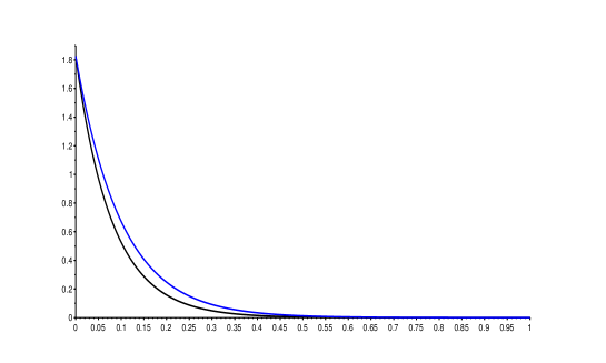
Figure 1: Time-evolution of $\|y^{*}(t)\|$ under the optimal control $u^{*}$ (black line) and the zero control $v_{1}=0$ (blue line).

Time (t)	0.2	0.3	0.6
$\|y^{*}(t)\|$	$15.8*10^{-2}$	$4.79*10^{-2}$	$1.2*10^{-3}$
$\|y_{v_{1}}(t)\|$	$24.8*10^{-2}$	$9.12*10^{-2}$	$4.56*10^{-3}$
$J(u^{*})$	$14.68*10^{-2}$	$14.77*10^{-2}$	$14.77*10^{-2}$
$J(v_{1})$	$16.38*10^{-2}$	$16.63*10^{-2}$	$16.67*10^{-2}$
$J(v_{2})$	$4.19$	$4.21$	$4.22$

Remark 5

Note that the stabilization problem of non-homogeneous distributed bilinear systems has been only considered for bounded control operator (see [2, 9, 10, 17]). Thus the existing results from the above literature are not applicable as here, the control operator $B$ is unbounded. Moreover, even in the homogeneous case (i.e $b=0$), the existing results for unbounded operator $B$ (see [4, 8]) are not applicable as here, the operator $B$ is skew adjoint. In particular, the observation inequality is not verified. Now, if we formally consider the feedback control $v(t)$ used in [4, 8], then we find $v(t)=0$ as $v(t)$ involves the term $\langle By,y\rangle$ which is null when $B$ is skew-adjoint.

V Conclusion

In this work, we studied the quadratic optimal control problem for a class of non-homogeneous bilinear Fokker-Planck equation. Both finite and infinite horizon cases are considered. It is further showed that the infinite horizon optimal control leads to a stabilized state of the system in closed-loop. This study provided a stabilization result which does not require the observation assumption. The result of Theorem 5 is promising. Indeed one can be inspired by it to investigate the optimal stabilization of a general unbounded bilinear system.

References

• [1] A. Addou and A. Benbrik.(2002) Existence and uniqueness of optimal control for a distributed parameter bilinear system, J. Dyn. Control Syst., 8, 141–152.
• [2] M, Akkouchi, & A. Bounabat (2003). Weak stabilizability of a nonautonomous and non-linear system. Mathematica Pannonica, 55, 61.
• [3] M. S. Aronna, & F. Tröltzsch (2021). First and second-order optimality conditions for the control of Fokker-Planck equations. ESAIM: Control, Optimisation and Calculus of Variations, 27, 15.
• [4] R. E. Ayadi, M. Ouzahra, & A. Boutoulout. (2012) Strong stabilisation and decay estimate for unbounded bilinear systems. International journal of control, 85(10), 1497-1505.
• [5] J. M. Ball, J. E. Marsden and M. Slemrod. (1982) Controllability for distributed bilinear systems, SIAM J. Control Optim., 20, 575–597.
• [6] S. Banks and M. Yew. (1985) On a class of suboptimal controls for infinite-dimensional bilinear systems, Systems and Control Letters, 5, 327–333.
• [7] L. Berrahmoune. (2009) A note on admissibility for unbounded bilinear control systems, Bulletin of the Belgian Mathematical Society-Simon Stevin, 16 , 193–204.
• [8] L. Berrahmoune. (2010). Stabilization of unbounded bilinear control systems in Hilbert space. Journal of mathematical analysis and applications, 372(2), 645-655.
• [9] H. Bounit, & H. Hammouri. (1999). Feedback stabilization for a class of distributed semilinear control systems. Nonlinear Analysis: Theory, Methods & Applications, 37(8), 953-969.
• [10] H. Bounit. (2003) Comments on the feedback stabilization for bilinear control systems. Applied mathematics letters, 16(6), 847-851.
• [11] M. E. Bradly and S. Lenhart. (1994) Bilinear optimal control of a Kirchhoff plate, Syst. Control Lett., 22, 27–38.
• [12] A. Bensoussan, G. Da Prato, M.C. Delfour and S.K. Mitter. (2007)Representation and Control of Infinite Dimensional Systems, Birkhaüser, Boston.
• [13] H. Brezis (1987) Analyse fonctionnelle : Théorie et applications, Paris, Masson.
• [14] J. M. Clérin. (2009) Problèmes de contrôle optimal du type bilinéaire gouvernés par des équations aux dérivées partielles d’évolution, Doctoral dissertation.
• [15] N. El Alami.(1986) Analyse et commande optimale des systèmes bilinéaires distribués, application aux procédés energétiques, Doctorat d’Etat-I.M.P. Perpignan, 1986.
• [16] A. Fleig and R. Guglielmi. (2016) Bilinear optimal control of the Fokker-Planck equation, IFAC-PapersOnLine, 49, 254–259.
• [17] Z. Hamidi, & M. Ouzahra. (2018). Partial stabilisation of non-homogeneous bilinear systems. International Journal of Control, 91(6), 1251-1258.
• [18] R. E. Kalman. (1960) Contributions to the theory of optimal control, Bol. Soc. Mat. Mexicano, 2, 102–119.
• [19] N. A. Krall, & A. W. Trivelpiece. (1973). Principles of plasma physics. American Journal of Physics, 41(12), 1380-1381.
• [20] X. Li and J. Yong. (2012) Optimal control theory for infinite dimensional systems, Springer Science $\&$ Business Media.
• [21] M. Ouzahra. (2007) Stabilization with Decay Estimate for a Class of Distributed Bilinear Systems, European Journal of Control, 5 509–515.
• [22] A. Pazy. (1983) Semi-groups of Linear Operators and Applications to Partial Differential Equations, Springer-Verlag, New York.
• [23] L. S. Pontryagin, V. G. Boltanski, R. V. Gamkrelidze and E. F. Mischenko (1962) Mathematical theory of optimal processes, Wiley, New York.
• [24] J.P. Quinn. (1982) Stabilization of bilinear systems by quadratic feedback control, J. Math. Anal. Appl, 75 66–80.
• [25] E. P. Ryan. (1984) Optimal feedback control of bilinear systems, Journal of Optimization Theory and Applications, 44 333–362.
• [26] C. S. Chen. (2009) Quadratic optimal neural fuzzy control for synchronization of uncertain chaotic systems, Expert Systems with Applications, 36 11827–11835.
• [27] S. Yahyaoui and M. Ouzahra. (2021) Quadratic optimal control and feedback stabilization of bilinear systems, Optimal Control Applications and Methods, https://doi.org/10.1002/oca.2704.
• [28] E. Zerrik and N. El Boukhari. (2019) Regional optimal control for a class of semilinear systems with distributed controls, International Journal of Control, 92 896–907
• [29] E. Zerrik and N. El Boukhari. (2018) Constrained optimal control for a class of semilinear infinite dimensional Systems, Journal of Dynamical and Control Systems, 24 65–81.