A study of latent monotonic attention variants

Abstract

End-to-end models reach state-of-the-art performance for speech recognition, but global soft attention is not monotonic, which might lead to convergence problems, to instability, to bad generalisation, cannot be used for online streaming, and is also inefficient in calculation. Monotonicity can potentially fix all of this. There are several ad-hoc solutions or heuristics to introduce monotonicity, but a principled introduction is rarely found in literature so far. In this paper, we present a mathematically clean solution to introduce monotonicity, by introducing a new latent variable which represents the audio position or segment boundaries. We compare several monotonic latent models to our global soft attention baseline such as a hard attention model, a local windowed soft attention model, and a segmental soft attention model. We can show that our monotonic models perform as good as the global soft attention model. We perform our experiments on Switchboard 300h. We carefully outline the details of our training and release our code and configs.

1 Introduction

The conventional hidden Markov model (HMM), including the hybrid neural network (NN) / HMM (Bourlard & Morgan, 1990; Robinson, 1994) is a time-synchronous model, which defines a probability per input frame (either $p(x_{t}|y_{t})$ or $p(y_{t}|x_{t})$). As such, it implicitly enforces monotonicity. Connectionist temporal classification (CTC) (Graves et al., 2006) can be seen as a special case of this (Zeyer et al., 2017). Generalisations of CTC are the recurrent neural network transducer (RNN-T) (Graves, 2012; Battenberg et al., 2017) or the recurrent neural aligner (Sak et al., 2017; Dong et al., 2018) or further extended generalized variations of the transducer (Zeyer et al., 2020).

The encoder-decoder-attention model (Bahdanau et al., 2014) is becoming one of the most competitive models for speech recognition (Chiu et al., 2018; Zeyer et al., 2018b; Park et al., 2019; Tüske et al., 2020). This model directly models the posterior probability $p(y_{1}^{N}|x_{1}^{T})$ for the output labels $y_{1}^{N}$ (word sequence), given the input sequence $x_{1}^{T}$ (audio features). This is factorised into $\prod_{i}p(y_{i}|y_{1}^{i-1},x_{1}^{T})$. We call this a label-synchronous model (sometimes also called direct model) because each NN output corresponds to one output label. This is in contrast to the time-synchronous models like hybrid NN/HMM, CTC and RNN-T. The encoder-decoder (label-sync.) model usually uses global soft attention in the decoder. I.e. for each output label $i$, we access the whole input sequence $x_{1}^{T}$. This global soft attention mechanism is inefficient (time complexity $O(T\cdot N)$) and can violate monotonicity.

Monotonicity is necessary to allow for online decoding. Also, for monotonic sequence-to-sequence tasks like speech recognition, a model which is enforced to be monotonic might converge faster, and should be more stable in decoding. In this work, we want to introduce monotonicity in a mathematically clean way by introducing a latent variable which presents the position in the audio (or frame-wise encoder).

2 Related work

Several approaches exists to introduce monotonicity for label-synchronous models. We categorize these different approaches and outline their advantages and disadvantages.

2.1 Soft constraints: By training, or by attention energy tendency

Monotonicity can be encouraged by the model (e.g. by modeling the attention energy computation in such a way that it tends to be monotonic) or during training (by additional losses, or some initialization with linear alignment) (Tachibana et al., 2018; Zhang et al., 2018). While these help for convergence, these are soft constraints, or just guidance, i.e. the model still can violate monotonicity.

2.2 Hybrids of attention and CTC/RNN-T

The idea is that a time-synchronous model like CTC or RNN-T enforces the monotonicity, and the attention model contributes for better performance (Watanabe et al., 2017; Hori et al., 2017; Kim et al., 2017; Moritz et al., 2019b, a; Miao et al., 2019; Chiu et al., 2019). Often there is a shared encoder, and one CTC output layer and another common decoder with attention, and the decoding combines both the CTC and the attention decoder. The decoding can be either implemented in a time-synchronous way or in a label-synchronous way. Depending on the specific details of the model and decoding, monotonicity is strictly enforced or just strongly encouraged (but it could happen that the attention scores dominate over the CTC model or so). These models usually perform quite well. However both the model and the decoding procedure become more complicated, and often rely on several heuristics. And it can be seen as a model combination, which makes the performance comparison somewhat unfair to single models.

2.3 Deterministic methods

Monotonicity can be introduced in a more conceptional way via deterministic methods, which model explicitly the source position (Graves, 2013; Luong et al., 2015; Tjandra et al., 2017; Hou et al., 2017; Jaitly et al., 2016; Raffel et al., 2017; Chiu & Raffel, 2017; Fan et al., 2018; Miao et al., 2019; Merboldt et al., 2019; He et al., 2019; Zhang et al., 2019). These approaches all provide strict monotonicity by using some position scalar (e.g. for a running window over the encoder output), and it is enforced that the position can only increase. In these approaches, the position is not interpreted as a latent variable, but it is rather calculated by a deterministic function given the current state of the decoder. These can be fully differentiable (if the position is a real number scalar) or rely on heuristics/approximations (if the position is a discrete number). This includes the implicit assumption that there exists a deterministic method which determines the position for the next label. We argue that this is a too strong assumption. In practice, given some history of input (audio) and previous labels (words), the model cannot tell for sure where the next label will occur. The model eventually can only estimate a probability or score. And later in decoding, after a few more input frames or words, we might see that the model did a wrong choice for the position. The beam search should be able to correct this, which is not possible if it is simply a deterministic function. If it cannot correct it, then the performance will have a bottleneck at this deterministic function, because when its estimate is bad or wrong, the further decoding will be affected consequently. MoChA (Chiu & Raffel, 2017) is probably one of the most prominent examples in this category. As it still does soft attention within one chunk, it can compensate bad chunk positions to some degree but not fully.

2.4 Latent variable models

A variety of works have introduced an explicit latent variable to model the alignment. We always have and even need this for hybrid NN/HMM models, CTC and RNN-T. One example of early label-synchronous models which have such a latent variable are the segmental conditional random fields (CRF) (Ostendorf et al., 1996; Zweig & Nguyen, 2009; Lu et al., 2016). The latent variable is usually discrete, and often represents the position in the encoder, or the segment boundaries. We will categorize the model for the latent variable by dependency orders in the following.

2.4.1 0-order models

The probability distribution of the latent variable can be independent from its history (0 order) (Bahuleyan et al., 2017; Shankar et al., 2018; Shankar & Sarawagi, 2019; Deng et al., 2018; Wu et al., 2018). The marginalisation over the latent variable becomes simple and efficient in that case and can easily be done in both training and decoding. However, it does not allow for strong alignment models, and also does not allow to constrain for monotonicity, because that would add a dependence on the history and then it is not 0-order anymore.

2.4.2 1st order models

If the probability distribution of the latent variable depends only on its predecessor, then it is of 1st order (Yu et al., 2016b, a; Wang et al., 2017, 2018; Alkhouli et al., 2016; Beck et al., 2018a, b). A first-order dependency allows to directly enforce monotonicity. The full marginalisation can still be calculated efficiently for 1st order models using dynamic programming (Yu et al., 2016b; Wang et al., 2018)

2.4.3 Higher order models

The probability distribution of the latent variable can also depend on more than just the predecessor, or even on the full history (Mnih et al., 2014; Ba et al., 2014; Xu et al., 2015; Vinyals et al., 2015; Lawson et al., 2018; Arivazhagan et al., 2019; Alkhouli & Ney, 2017; Alkhouli et al., 2018). This is often the case if some recurrent decoder is used and the probability distribution depends on that state, which itself depends on the full history. The full marginalisation becomes infeasible for higher order, thus requires further approximations such as the maximum approximation (Alkhouli & Ney, 2017; Alkhouli et al., 2018).

2.4.4 Decoding with first or higher-order latent variable models

Only few other work includes the latent variable in beam search during decoding (Yu et al., 2016b, a; Wang et al., 2018; Alkhouli et al., 2016; Alkhouli & Ney, 2017; Alkhouli et al., 2018; Beck et al., 2018a) while most other work uses sampling or a greedy deterministic decision during decoding, which again leads to all the problems outlined in Section 2.3. We argue that we should properly search over the latent variable space and incorporate that into the beam search decoding procedure such that the decoding can correct wrong choices on the latent variable. Also this is mostly straight forward and mathematically clean.

Note that if we simplify the beam search to simply pick the $\operatorname*{arg\,max}$ for the latent variable in each decoder step, we get back to deterministic models. In that sense, latent variable models are a strict generalization of all the deterministic approaches.

3 This work: our latent variable model

We conceptually introduce monotonicity in a mathematically clean way to our label-synchronous encoder-decoder model by a discrete latent variable which represents the position (or segment boundary) in the audio (or frame-wise encoder). We now have several options for the model assumptions. For the monotonicity, we at least need a model of 1st order. We make it higher order and depend on the full history. This is is a trade-off between a more powerful model and more approximations needed in decoding and training, such as the maximum approximation. The maximum approximation has successfully and widely been used for speech recognition in different scenarios such as decoding and Viterbi training for hybrid NN/HMM models (Yu & Deng, 2014). This is why we think the maximum approx. should be fine for label-sync. models as well. And on the other side, a more powerful model could improve the performance.

We argue that these models with a latent variable are conceptually better founded than the deterministic models which rely on heuristics without good mathematical justification. In addition, in such an approach, the conventional maximum approximation can be naturally introduced to achieve efficient and simple training and decoding.

As we want to understand the effect of this latent variable, and the hard monotonicity constrain on it, we want to keep the differences to our baseline encoder-decoder model with global soft attention as small as possible. This means that we still have a bidirectional long short-term memory (LSTM) (Hochreiter & Schmidhuber, 1997) encoder and an offline feature extraction pipeline is offline. There is a wide range of existing work on making these missing parts online capable (Zeyer et al., 2016; Peddinti et al., 2017; Xue & Yan, 2017). In all our latent models, the added latent variable represents either:

• a single discrete position in the encoder output,

• a discrete center position of a window over the encoder output,

• or a segment boundary on the encoder output.

To further keep the difference to the baseline small, the probability of the latent variable is simply given by the attention weights (but masked to fulfil monotonicity). Also the remaining part of the decoder is kept exactly the same, except of how we calculate the attention context, which is not by global soft attention anymore. We do not improve on the runtime complexity in this work, to stay closer to the baseline for a better comparision. However, it is an easy further step to make the runtime linear, as we will outline later.

Also, in the existing works, the final model properties are rarely discussed beyond the model performance. We perform a systematic study of different properties of our latent variable models, considering modeling, training, and decoding aspects.

The experiments were performed with RETURNN (Zeyer et al., 2018a), based on TensorFlow (Abadi et al., 2015). All the code and the configs for all our experiments is publicly available.

4 Models

We use a LSTM-based global soft attention model similar to (Bahdanau et al., 2014; Luong et al., 2015; chorowski2015attention; chan2016las; bahdanau2016endtoendasr). In all cases, the model consists of an encoder, which learns a high-level representation of the input signal $x_{1}^{T}$,

$$h_{1}^{T^{\prime}}=\operatorname{Encoder}(x_{1}^{T}).$$

We apply time downsampling, thus we have $T^{\prime}\leq T$. In our case, it is a bidirectional LSTM with time-max-pooling. The global soft attention model defines the probability

$$p(y_{1}^{N}|x_{1}^{T})=\prod_{i=1}^{N}p(y_{i}|y_{1}^{i-1},x_{1}^{T})$$

with

$$p(y_{i}|y_{1}^{i-1},x_{1}^{T})=p(y_{i}|y_{1}^{i-1},h_{1}^{T^{\prime}})=p(y_{i}|y_{1}^{i-1},c_{1}^{i}),$$

for $i\in\{1,\dots,N\}$, where $c_{i}$ is the attention context vector. We get the dependence on the full sequence $c_{1}^{i}$ because we use a recurrent NN.

4.1 Baseline: Global soft attention

There is no latent variable. The attention context $c_{i}$ is calculated as

$$c_{i}=\sum_{t=1}^{T^{\prime}}\alpha_{i,t}(y_{1}^{i-1},\alpha_{1}^{i-1},c_{1}^{i-1})\cdot h_{t},$$

and the attention weights $\alpha_{i}$ are a probability distribution over $\{1,\dots,T^{\prime}\}$, which we calculate via MLP-attention (Bahdanau et al., 2014; Luong et al., 2015). In this model, there is no explicit alignment between an output label $y_{i}$ and the input $x_{1}^{T}$ or the encoder output $h_{1}^{T^{\prime}}$. However, the attention weights can be interpreted as a soft alignment. The model also uses weight feedback (Tu et al., 2016).

The model is trained by minimising the negative log probability over the training dataset $\mathcal{D}$

$$L=-\sum_{(x,y)\in\mathcal{D}}\sum_{i=1}^{N}\log p(y_{i}|y_{1}^{i-1},x_{1}^{T}).$$

We also use a pretraining scheme such as growing the model size, which we outline in the experiments section. Decoding is done by searching for

$$\operatorname*{arg\,max}_{N,y_{1}^{N}}\sum_{i=1}^{N}\log p(y_{i}|y_{1}^{i-1},x_{1}^{T})$$

which is approximated using label-synchronous beam search.

4.2 Latent models

When introducing a label-synchronous discrete latent variable $t_{i}$ for all $i\in\{1,\dots,N\}$, we get

$$p(y_{1}^{N}|x_{1}^{T}) =\sum_{t_{1}^{N}}p(y_{1}^{N},t_{1}^{N}|x_{1}^{T})$$

$$=\sum_{t_{1}^{N}}\prod_{i=1}^{N}p(y_{i},t_{i}|y_{1}^{i-1},t_{1}^{i-1},x_{1}^{T})$$

$$=\sum_{t_{1}^{N}}\prod_{i=1}^{N}p(y_{i}|y_{1}^{i-1},t_{1}^{i},x_{1}^{T})p(t_{i}|y_{1}^{i-1},t_{1}^{i-1},x_{1}^{T}).$$

Analogous to the baseline, we use

$$p(y_{i}|y_{1}^{i-1},t_{1}^{i},x_{1}^{T})=p(y_{i}|y_{1}^{i-1},c_{1}^{i}),$$

where the attention context $c_{i}$ depends also on $t_{i}$ now.

We construct the model in a way that the access to $h_{1}^{T^{\prime}}$ via $t_{i}$ is monotonic by $t_{i}\leq t_{i+1}$ or even $t_{i}<t_{i+1}$. In every case, the model is trained again by minimising the negative log probability, and using the max. approximation for $\sum_{t_{1}^{N}}$,

$$L=-\sum_{(x,y)\in\mathcal{D}}\max_{t_{1}^{N}}\sum_{i=1}^{N}\log p(y_{i},t_{i}|y_{1}^{i-1},t_{1}^{i-1},x_{1}^{T}).$$

The $\operatorname*{arg\,max}_{t_{1}^{N}}$ is further approximated by beam search, which is also called forced alignment or Viterbi alignment. Also, in all cases, we try to be close to the global soft attention model, such that a comparison is fair and direct, and even importing model parameters is reasonable.

The probability for the latent variable $t_{i}$ is simply given by the attention weights

$$p(t_{i}=t|y_{1}^{i-1},t_{1}^{i-1},x_{1}^{T})=\alpha^{\prime}_{i,t}$$

with $\alpha^{\prime}_{i,t}=0\quad\forall t<t_{i-1}$. The attention weights in this case are masked to fulfil monotonicity ($t<t_{i-1}$ if we want strict monotonicity, else $t\leq t_{i-1}$), and $\alpha^{\prime}_{i,t}\propto\alpha_{i,t}$ renormalised accordingly. We choose this model $p(t|\dots)$ based on the attention weights to keep a strong similarity to the baseline model. However, because of this model, we still have $O(T\cdot N)$ runtime complexity. In future work, we can further deviate from this, and compare to other models for $p(t|\dots)$ which allow for linear runtime $O(T+N)$ or even $O(T)$. E.g. an obvious alternative is to use a Bernoulli distribution and to define it frame-wise, not globally over all frames.

In all latent models, we define the attention context $c_{i}$ as

$$c_{i}=\sum_{t=w_{i}}^{w^{\prime}_{i}}\alpha^{\prime\prime}_{i,t}\cdot h_{t},$$ (1)

i.e. we use soft attention on a window $[w_{i},w^{\prime}_{i}]$ (or hard, if it is a single frame), for some $\alpha^{\prime\prime}$ as described in the following.

Decoding is done by searching for

$$\operatorname*{arg\,max}_{N,y_{1}^{N},t_{1}^{N}}\sum_{i=1}^{N}\log p(y_{i},t_{i}|y_{1}^{i-1},t_{1}^{i-1},x_{1}^{T})$$

which is approximated using label-synchronous beam search.

4.3 Monotonic hard attention

By simply setting $[w_{i},w^{\prime}_{i}]=[t_{i},t_{i}]$ in Equation 1, we have the attention only on a single frame, and simply $\alpha^{\prime\prime}_{i,t}=1$. This can be interpret as hard attention instead of soft attention, and $t_{i}$ is the position in $h_{1}^{T^{\prime}}$. Everything else stays as before. There are multiple motivations why to use hard attention instead of soft attention:

• The model becomes very simple.

• In the global soft attention case, we can experimentally see that the attention weights are usually very sharp, often focused almost exclusively on a single frame.

4.4 Monotonic local windowed soft attention

We use $[w_{i},w^{\prime}_{i}]=[t_{i}-D_{l},t_{i}+D_{r}]$ for fixed $D_{l},D_{r}$. In this case, the latent variable $t_{i}$ is the center window position, and $\alpha^{\prime\prime}_{i,t}\propto\alpha_{i,t}$ renormalised on the window. This model is very similar to (Merboldt et al., 2019) but with a latent variable.

4.5 Monotonic segmental soft attention

Here we make use of the latent variable $t_{i}$ as the segment boundary, i.e. we use $[w_{i},w^{\prime}_{i}]=[t_{i-1}+1,t_{i}]$. Here, we have a separate model for $\alpha^{\prime\prime}_{i,t}$, which are separately computed MLP soft attention weights.

5 Training procedure for latent models

For one training sample $(x,y)\in\mathcal{D}$, the loss we want to minimise is

$$L=-\max_{t_{1}^{N}}\log p(y_{i}^{N},t_{i}^{N}|x_{1}^{T}),$$

i.e. we have to calculate $\arg\max_{t_{1}^{N}}$, i.e. search for the best $t_{1}^{N}$, which we call alignment. This is the maximum approximation for training. This can be done using dynamic programming (beam search, Viterbi). We could also decouple the search for the best alignment from updating the model parameters, but in our experiments, we always do the search online on-the-fly, i.e. in every single mini-batch, it uses the current model for the search. We note that this beam search is exactly the same beam search implementation which we use during decoding, but we keep the ground truth $y_{1}^{N}$ fixed, and only search over the $t_{1}^{N}$.

For stable training, we use the following tricks, which are common for other models as well, but adopted now for our latent variable models.

• The maximum approximation can be problematic in the very beginning of the training, when the model is randomly initialized. In the case of HMM models, it is common to use a linear alignment in the beginning, instead of calculating the Viterbi alignment ($\operatorname*{arg\,max}_{t_{1}^{N}}$). We do the same for our latent variable models.

• We store the last best alignment (initially the linear alignment) and its score. When we calculate a new Viterbi alignment, we compare the score to the previous best score, and update the alignment if the score is better. This greatly enhances the stability early in training, esp. when we still grow the model size in pretraining.

• We can use normal global soft attention initially. Note that this is still slightly different compared to the global soft attention baseline because of the other small differences in the model, such as different (hard) weight feedback.

Given an existing alignment $t_{1}^{N}$ for this training example, the loss becomes

$$L=\sum_{i=1}^{N}-\log p(y_{i}|y_{1}^{i-1},c_{1}^{i})-\log p(t_{i}|y_{1}^{i-1},c_{1}^{i-1}).$$

We note that this is the same loss as before, with the additional negative log likelihood for $p(t_{i}|\dots)$. We can also easly introduce a different loss scale for each log likelihood. We use the scale $0.1$ by default for $p(t_{i}|\dots)$.

As we do the search for the optimal $t_{1}^{N}$ on-the-fly during training, this adds to the runtime and makes it slower. However, on the other side, the model itself can be faster, depending on the specific implementation. In our case, for the hard attention model, we see about 40% longer training time. If we would use a fixed alignment $t_{1}^{N}$, it would actually be faster to train than the baseline.

6 Decoding with latent variable

The decoding without an additional latent variable is performed as usual, using label synchronous beam search with a fixed beam size (Sutskever et al., 2014; Bahdanau et al., 2014; Zeyer et al., 2018a). When we introduce the new latent variable into the decoding search procedure, the beam search procedure stays very similar. We need to search for

$$\operatorname*{arg\,max}_{N,y_{1}^{N},t_{1}^{N}}\sum_{i=1}^{N}\log p(y_{i}|y_{1}^{i-1},c_{1}^{i})+\log p(t_{i}|y_{1}^{i-1},c_{1}^{i-1}).$$

As $p(y_{i}|\dots)$ depends on $t_{i}$ (via $c_{i}$), in any decoder step $i$, we first need to hypothesize possible values for $t_{i}$, and then possibe values for $y_{i}$, and then repeat for the next $i$. We have two beam sizes, $K_{y}$ and $K_{t}$ for $p(y|\dots)$ and $p(t|\dots)$ respectively.

The expansion of the possible choices for $t_{i}$ is simply analogous as for the output label $y_{i}$: We fully expand all possible values for $t_{i}$, i.e. calculate the score $p(t_{i}{=}t|\dots)\cdot p(y_{i}^{i-1},t_{1}^{i-1}|x_{1}^{T})$ for all possible $t$, for all current active hypotheses, just as we do for $y$. However, we have various options for when, what and how do we apply pruning. After we calculated the scores for $y_{i}$, based on the joint scores $p(y_{i}{=}y|\dots)\cdot p(y_{i}^{i-1},t_{1}^{i}|x_{1}^{T})$, we prune to the best $K_{y}$ hypotheses. Now on the choice of $t_{i}$, we have $K\cdot T^{\prime}$ active hypotheses, where $K=1$ at the beginning, and then $K=K_{y}$. For pruning the hypotheses on $t_{i}$ based on the joint scores $p(t_{i}{=}t|\dots)\cdot p(\dots)$:

• We either select the overall $K_{t}$ best, ending up with $K_{t}$ hypotheses.

• Or for each previous hypotheses (last choice on $y_{i-1}$), we select the best $K^{\prime}_{t}$ choices for $t_{i}$, ending up with $K_{t}=K\cdot K^{\prime}_{t}$ hypotheses. I.e. we only expand and don’t prune $y_{1}^{i-1}$ hypotheses away at this point, but only prune away new choices of $t_{i}$, i.e. take the top-$K^{\prime}_{t}$ of possible $t_{i}$ values.

As a further approximation, we can also discard hypotheses in the beam which have the same history $y_{1}^{i}$ but a different history $t_{1}^{i}$. We currently do this for the Viterbi alignment during training with ground truth, such that we only consider

$$t_{i}\mapsto\max_{t_{1}^{i-1}}p(t_{i}|\dots)\cdot p(y_{1}^{i-1},t_{1}^{i-1}|x_{1}^{T}).$$

We do not use this for decoding yet. In general, this can make more efficient use of the beam.

Note that this is in the worst case only slower to the baseline by some small constant factor. In practice, in the batched GPU-based beam search which we do, we do not see any difference. Once we use different models for $p(t|\dots)$, we can even potentially gain a huge speedup.

7 Experiments

Table 1: Overall comparisons of models. We use the beam sizes $K_{y}=12$ and $K_{t}=48$ with expand on $t$ as explained in Section 6. The frame error rate (FER) is calculated on the labels, feeding in the ground truth seq., on some cross-validation set. The latent models all import the global soft. att. baseline, which screws the effective num. of epochs though, as the model is changed drastically.

Model Effect. WER[%] FER num. Hub5’00 Hub5’01 [%] ep. $\Sigma$ SWB CH $\Sigma$ Global soft. 033.3 15.3 10.1 20.5 14.9 8.5 066.7 14.3 09.3 19.3 14.0 8.0 100.0 14.4 09.1 19.7 13.9 8.0 Segmental 058.3 15.7 09.9 21.5 14.6 7.4 083.3 15.7 10.1 21.3 14.9 6.9 Hard att. 033.3 15.8 10.3 21.3 15.4 7.3 050.0 15.1 09.7 20.5 14.8 7.3 091.7 14.4 09.3 19.5 14.2 7.0 Local win. 033.3 15.4 10.2 20.5 14.9 8.0 050.0 14.7 09.4 20.0 14.1 7.7 083.3 14.4 09.1 19.7 13.8 7.6

7.1 Dataset & global soft attention baseline

All our experiments are performed on Switchboard (Godfrey et al., 1992) with 300h of English telephone speech. We use SpecAugment (Park et al., 2019) for data augmentation. We have two 2D-convolution layers, followed by 6 layer bidirectional LSTM encoder of dimension 1024 in each direction, with two time-max-pooling layers which downsample the time dimension by a factor of 6 in total. Our output labels are 1k BPE subword units (Sennrich et al., 2015). All our experiments are without the use of an external language model. We use a pretraining/training-scheduling scheme which

• starts with a small encoder, consisting of 2 layers and 512 dimensions, and slowly grows both in depth (number of layers) and width (dimension) up until the final model size,

• starts with reduced dropout rates, which are slowly increased,

• starts without label smoothing, and only later enables it,

• starts with a less strong SpecAugment,

• starts with a higher batch size.

This scheme is performed during the first 10 full epochs of training. In addition, for the first 1.5 epochs, we do learning rate warmup, and after that we do the usual learning rate scheduling (Bengio, 2012). After every 33.3 epochs, we do a reset of the learning rate. We show the performance in Table 1. We see that longer training time can yield drastic improvements. We train these experiments using a single Nvidia GTX 1080 Ti, and one epoch takes about 3h-6h, depending on the model.

7.2 Latent variable models

7.2.1 Pretraining scheme

Table 2: From scratch vs imported initialization, for hard attention and local windowed soft attention. WER on Hub5’00.

Model Imported baseline, Effective WER num. of ep. num. of ep. [%] Hard att. — 33.3 15.8 33.3 58.3 15.1 66.7 91.7 14.4 Local win. — 33.3 15.4 33.3 50.0 15.1

As all our proposed models are close to the global soft attention baseline, we can import the model parameters from the baseline and fine tune. With the aforementioned methods for stable training such as reusing the previously best alignment, we are also able to train from scratch, as we show in Table 2. Note that the difference in “from scratch” training to importing a baseline is somewhat arbitrary here, because the latent variable models also use some pretraining scheme as outlined in Section 5. Thus we end up with two different kinds of pretraining schedules, and “from scratch” training uses much less global soft attention during pretraining. This merely demonstrates that from scratch training is possible, i.e. that we can switch to a fully latent model (without global soft attention) already early in training. The performance difference in these experiments might also just be due to the different effective number of epochs. Note that ultimately after the switch from the global soft attention model to a latent variable model, we will always see a drop in WER, as the model is not the same. The amount of this degradation can be seen in Table 6. In the following experiments we use the best possible scheduling, which currently imports existing global soft attention models.

7.2.2 Prune variants in decoding

Table 3: Comparison on different decode pruning on $t_{i}$, for a hard attention model. We always use the beam size $K_{y}=12$. Expand as explained in Section 6, and $K_{t}$ is the beam size after the choice on $t_{i}$. In the case of expand with $K_{t}=K_{y}$, we get the deterministic $\operatorname*{arg\,max}_{t_{i}}$ approach. WER on Hub 5’00.

Model Expand $t_{i}$ $K_{t}$ WER[%] Hard att. yes 12 14.8 24 14.5 48 14.4 96 14.4 no 12 14.5 24 14.4 48 14.4 96 14.4 Local win. yes 12 14.7 48 14.7 96 14.7 no 12 14.8 48 14.7 96 14.7

Table 4: Comparison on different $\alpha$ for $p(t|\dots)^{\alpha}$ and softmax temperature for a hard attention model. We always use the beam size $K_{y}=12$, $K_{t}=48$, and expand $t_{i}$ (Section 6). WER on Hub 5’00.

Softmax temp. $p(t)$ scale $\alpha$ WER[%] 1.0 0.1 21.2 0.5 14.5 1.0 14.4 1.5 14.6 0.5 1.0 14.5 1.5 1.0 14.6

We analyse the different kinds of pruning on the latent variable $t_{i}$ during decoding, and the beam size $K_{t}$, as explained in Section 6. Results are collected in Table 3. The results indicate that we need a large enough beam size for optimal performance. For the hard attention model, a simple deterministic decision on $t_{i}$ is slightly worse than doing beam search on it. It does not seem to matter too much for the local windowed attention model, which probably can recover easily if the choice on $t_{i}$ is slightly off. Note that this is very much dependent on the quality of the model $p(t|\dots)$. If that model is weak, it should be safer and better to use the expand prune variant with some $K_{t}>K_{y}$, as it would not prune away possibly good $y_{1}^{i}$ hypotheses. However, our experiments do not demonstrate this yet, which could be simply due to an already powerful model. In our experiments $K_{y}=12$, $K_{t}=K_{y}\cdot K^{\prime}_{t}=48$, i.e. $K^{\prime}_{t}=4$ seems to be enough. That means that we effectively consider always the top 4 scored choices for $t_{i}$. We also did experiments on overall larger beam sizes for $K_{y}$ as well but do not see any further improvement. We also experimented with an exponent on the probability, i.e. $p(t|\dots)^{\alpha}$, but $\alpha\approx 1$ seems to perform best. We also tried different $\operatorname{softmax}$ temperature factors for $p(t|\dots)$, but again $1$ seems to be the optimum. These experiments are shown in Table 4. We note again that this behaviour is likely dependent on the specific kind of model $p(t|\dots)$.

7.2.3 Overall results

We collect the final results in Table 1. We again also report the total number of epochs of the training data which were seen. We also report the frame error rate (FER), which we found interesting, as it is consistently much better for all of the latent models. Our assumption is that the alignment procedure works well and it makes a good prediction of the output label easier, given the good position information. However, we do not see this for the WER. The segmental model seems to have the highest FER, while it performs not as good as the other latent models. This could be due to some overfitting effect, but needs further studying. We assume this is due to the exposure bias in training, where it always has seen the ground truth label sequence and a good alignment. The global soft attention model has less problems with this, as there is never a fixed alignment. Overall, the WERs of the latent models are competitive to global soft attention.

7.2.4 Restriction on the max step size $t_{i}-t_{i-1}$

Table 5: Comparison on different maximum step sizes for $p(t|\dots)$. WER on Hub 5’00. In the unlimited case, there can be step sizes over 150 frames (9s), although the mean step size is about 4.3 $\pm$ 4.0 frames (0.26s $\pm$ 0.24s).

Model Max. step size WER[%] Hard att. 10 (0.6s) 18.1 20 (1.2s) 14.7 30 (1.8s) 14.5 $\infty$ 14.4 Local win. 10 (0.6s) 14.6 20 (1.2s) 14.5 30 (1.8s) 14.5 $\infty$ 14.5

In all the experiments, the model $p(t|\dots)$ operates offline on the whole input sequence, and then calculates a $\operatorname{softmax}$ over the time dimension. For an online capable model, we cannot use $\operatorname{softmax}$ for the normalisation unless we restrict the maximum possible step size, which is maybe a good idea in general. Specifically, $p(t_{i}{=}t|\dots)=0$ for all $t>t_{i-1}+\Delta_{t}$ for some $\Delta_{t}$. We collected the results in Table 5. We can conclude that a maximum step size of 30 frames, which corresponds to 1.8 seconds, is enough, although this might depend on the dataset.

7.2.5 Further discussion

Table 6: Our incremental effort to tune the hard attention model. WER on Hub5’00. We report the WER directly after importing the baseline (without any update), for training begin (50h of training data), and then after that the best ($\geq$100h of training data). A connected cell in the table means that this number cannot have changed conceptually.

Incremental changes: WER[%] All changes from top to bottom base- after train further add up. line imp. begin best Starting point: no label smoothing, 15.3 18.7 17.0 19.1 no weight feedback, $K_{y}=K_{t}=12$ Weight feedback (soft att. weights), 16.5 16.9 16.9 lower learning rate, no lr. warmup Approximated recombination for 16.4 16.9 16.8 realignment, expand on $t$, $K_{t}=48$, $\log p(t|...)$ loss scale 0.1, accum. att. weights use hard att. Label smoothing ($0.1$) 16.4 16.2 Correct seq. shuffling 15.1 Higher learning rate, lr. warmup 14.8 Import better baseline 14.3 15.4 15.3 14.4

Achieving to the final results required multiple states of tuning. In Table 6, we share our development history up to the final results. The starting point does not use label smoothing, which was actually a bug and not intended. We see that label smoothing has a big positive effect. Even bigger was the effect by not shuffling the sequences, which was a bug as well. As we can see from the table, this makes an absolute WER difference of more than 1%. While it was never the intention to do that, we think it might still be interesting for the reader to follow the history of our development. We see that in our initial experiments, the training actually made the model worse, which can be explained by running into a bad local optimum due to an unstable alignment procedure. Fortunately the alignment procedure becomes more stable for the further experiments. The global soft attention baseline also used weight feedback, and it was not obvious whether the latent models should have that as well, and how exactly. We ended up in the variant that we use the hard choice on $t_{i}$ instead of the attention weights, and create a “hard” variant of accumulated weights, although it is not fully clear whether this is the optimal solution.

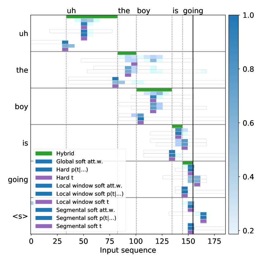
Figure 1: This figure shows the soft and hard attention weights, or segment boundaries of all the models, including a reference Viterbi alignment from a hybrid NN/HMM model. The light grey boxes mark the area where the attention weights or probability distribution is non-zero. Some of the models define the attention weights on a longer sequence, due to the downscaling, or additionally padded zeros at the end.

In Figure 1 we can see the different alignment behaviour and attention weights of each model. We can see that most models behave as intended. In this direct comparison, we see that the global soft attention is noticeably less sharp.

8 Conclusion & future work

We introduced multiple monotonic latent attention models and demonstrated competitive performance to our strong global soft attention baseline. From the low FER, we speculate that we have a stronger exposure bias problem now (not only the ground truth labels $y_{1}^{N-1}$ but also the time alignment $t_{1}^{N}$). This problem can be solved e.g. via more regularisation or different training criteria such as minimum WER training (Prabhavalkar et al., 2018) and we expect to get future improvements. By further tuning, eventually we expect to get consistently better than the global soft attention baseline. Future work will also include different alignment models as well as online capable encoders. Also, while we do label-synchronous decoding in this work, a latent variable model allows for time-synchronous decoding as well, which is esp. interesting the the context of online streaming.

References

- Abadi et al. (2015) Abadi, M., Agarwal, A., Barham, P., Brevdo, E., Chen, Z., Citro, C., Corrado, G. S., Davis, A., Dean, J., Devin, M., Ghemawat, S., Goodfellow, I., Harp, A., Irving, G., Isard, M., Jia, Y., Jozefowicz, R., Kaiser, L., Kudlur, M., Levenberg, J., Mané, D., Monga, R., Moore, S., Murray, D., Olah, C., Schuster, M., Shlens, J., Steiner, B., Sutskever, I., Talwar, K., Tucker, P., Vanhoucke, V., Vasudevan, V., Viégas, F., Vinyals, O., Warden, P., Wattenberg, M., Wicke, M., Yu, Y., and Zheng, X. TensorFlow: Large-scale machine learning on heterogeneous systems, 2015. URL https://www.tensorflow.org/. Software available from tensorflow.org.
- Alkhouli & Ney (2017) Alkhouli, T. and Ney, H. Biasing attention-based recurrent neural networks using external alignment information. In WMT, pp. 108–117, Copenhagen, Denmark, September 2017.
- Alkhouli et al. (2016) Alkhouli, T., Bretschner, G., Peter, J.-T., Hethnawi, M., Guta, A., and Ney, H. Alignment-based neural machine translation. In ACL, pp. 54–65, Berlin, Germany, August 2016.
- Alkhouli et al. (2018) Alkhouli, T., Bretschner, G., and Ney, H. On the alignment problem in multi-head attention-based neural machine translation. In WMT, pp. 177–185, Brussels, Belgium, October 2018.
- Arivazhagan et al. (2019) Arivazhagan, N., Cherry, C., Macherey, W., Chiu, C.-C., Yavuz, S., Pang, R., Li, W., and Raffel, C. Monotonic infinite lookback attention for simultaneous machine translation. arXiv preprint arXiv:1906.05218, 2019.
- Ba et al. (2014) Ba, J., Mnih, V., and Kavukcuoglu, K. Multiple object recognition with visual attention. arXiv preprint arXiv:1412.7755, 2014.
- Bahdanau et al. (2014) Bahdanau, D., Cho, K., and Bengio, Y. Neural machine translation by jointly learning to align and translate. arXiv preprint arXiv:1409.0473, 2014.
- Bahuleyan et al. (2017) Bahuleyan, H., Mou, L., Vechtomova, O., and Poupart, P. Variational attention for sequence-to-sequence models. arXiv preprint arXiv:1712.08207, 2017.
- Battenberg et al. (2017) Battenberg, E., Chen, J., Child, R., Coates, A., Li, Y. G. Y., Liu, H., Satheesh, S., Sriram, A., and Zhu, Z. Exploring neural transducers for end-to-end speech recognition. In ASRU, pp. 206–213. IEEE, 2017.
- Beck et al. (2018a) Beck, E., Hannemann, M., Doetsch, P., Schlüter, R., and Ney, H. Segmental encoder-decoder models for large vocabulary automatic speech recognition. In Interspeech, Hyderabad, India, September 2018a.
- Beck et al. (2018b) Beck, E., Zeyer, A., Doetsch, P., Merboldt, A., Schlüter, R., and Ney, H. Sequence modeling and alignment for LVCSR-systems. In ITG, Oldenburg, October 2018b.
- Bengio (2012) Bengio, Y. Practical recommendations for gradient-based training of deep architectures. In Neural networks: Tricks of the trade, pp. 437–478. Springer, 2012.
- Bourlard & Morgan (1990) Bourlard, H. and Morgan, N. A continuous speech recognition system embedding mlp into hmm. In Advances in neural information processing systems, pp. 186–193, 1990.
- Chiu & Raffel (2017) Chiu, C.-C. and Raffel, C. Monotonic chunkwise attention. arXiv preprint arXiv:1712.05382, 2017.
- Chiu et al. (2018) Chiu, C.-C., Sainath, T. N., Wu, Y., Prabhavalkar, R., Nguyen, P., Chen, Z., Kannan, A., Weiss, R. J., Rao, K., Gonina, E., et al. State-of-the-art speech recognition with sequence-to-sequence models. In 2018 IEEE International Conference on Acoustics, Speech and Signal Processing (ICASSP), pp. 4774–4778. IEEE, 2018.
- Chiu et al. (2019) Chiu, C.-C., Rybach, D., McGraw, I., Visontai, M., Liang, Q., Prabhavalkar, R., Pang, R., Sainath, T., Strohman, T., Li, W., He, Y. R., and Wu, Y. Two-pass end-to-end speech recognition. In Interspeech, 2019.
- Deng et al. (2018) Deng, Y., Kim, Y., Chiu, J., Guo, D., and Rush, A. Latent alignment and variational attention. In NeurIPS, pp. 9712–9724, 2018.
- Dong et al. (2018) Dong, L., Zhou, S., Chen, W., and Xu, B. Extending recurrent neural aligner for streaming end-to-end speech recognition in mandarin. arXiv preprint arXiv:1806.06342, 2018.
- Fan et al. (2018) Fan, R., Zhou, P., Chen, W., Jia, J., and Liu, G. An online attention-based model for speech recognition. arXiv preprint arXiv:1811.05247, 2018.
- Godfrey et al. (1992) Godfrey, J. J., Holliman, E. C., and McDaniel, J. Switchboard: Telephone speech corpus for research and development. In ICASSP, pp. 517–520, 1992.
- Graves (2012) Graves, A. Sequence transduction with recurrent neural networks. arXiv preprint arXiv:1211.3711, 2012.
- Graves (2013) Graves, A. Generating sequences with recurrent neural networks. arXiv preprint arXiv:1308.0850, 2013.
- Graves et al. (2006) Graves, A., Fernández, S., Gomez, F., and Schmidhuber, J. Connectionist temporal classification: labelling unsegmented sequence data with recurrent neural networks. In ICML, pp. 369–376. ACM, 2006.
- He et al. (2019) He, M., Deng, Y., and He, L. Robust sequence-to-sequence acoustic modeling with stepwise monotonic attention for neural TTS. arXiv preprint arXiv:1906.00672, 2019.
- Hochreiter & Schmidhuber (1997) Hochreiter, S. and Schmidhuber, J. Long short-term memory. Neural computation, 9(8):1735–1780, 1997.
- Hori et al. (2017) Hori, T., Watanabe, S., and Hershey, J. R. Joint CTC/attention decoding for end-to-end speech recognition. In Proceedings of the 55th Annual Meeting of the Association for Computational Linguistics (Volume 1: Long Papers), pp. 518–529, 2017.
- Hou et al. (2017) Hou, J., Zhang, S., and Dai, L.-R. Gaussian prediction based attention for online end-to-end speech recognition. In Interspeech, pp. 3692–3696, 2017.
- Jaitly et al. (2016) Jaitly, N., Le, Q. V., Vinyals, O., Sutskever, I., Sussillo, D., and Bengio, S. An online sequence-to-sequence model using partial conditioning. In NeurIPS, pp. 5067–5075, 2016.
- Kim et al. (2017) Kim, S., Hori, T., and Watanabe, S. Joint CTC-attention based end-to-end speech recognition using multi-task learning. In 2017 IEEE international conference on acoustics, speech and signal processing (ICASSP), pp. 4835–4839. IEEE, 2017.
- Lawson et al. (2018) Lawson, D., Chiu, C.-C., Tucker, G., Raffel, C., Swersky, K., and Jaitly, N. Learning hard alignments with variational inference. In ICASSP, 2018.
- Lu et al. (2016) Lu, L., Kong, L., Dyer, C., Smith, N. A., and Renals, S. Segmental recurrent neural networks for end-to-end speech recognition. arXiv preprint arXiv:1603.00223, 2016.
- Luong et al. (2015) Luong, M.-T., Pham, H., and Manning, C. D. Effective approaches to attention-based neural machine translation. arXiv preprint arXiv:1508.04025, 2015.
- Merboldt et al. (2019) Merboldt, A., Zeyer, A., Schlüter, R., and Ney, H. An analysis of local monotonic attention variants. In Interspeech, Graz, Austria, September 2019.
- Miao et al. (2019) Miao, H., Cheng, G., Zhang, P., Li, T., and Yan, Y. Online hybrid CTC/attention architecture for end-to-end speech recognition. In Interspeech, pp. 2623–2627, 2019.
- Mnih et al. (2014) Mnih, V., Heess, N., Graves, A., et al. Recurrent models of visual attention. In NeurIPS, pp. 2204–2212, 2014.
- Moritz et al. (2019a) Moritz, N., Hori, T., and Le Roux, J. Streaming end-to-end speech recognition with joint CTC-attention based models. In Proc. IEEE Workshop on Automatic Speech Recognition and Understanding (ASRU), 2019a.
- Moritz et al. (2019b) Moritz, N., Hori, T., and Le Roux, J. Triggered attention for end-to-end speech recognition. In ICASSP 2019-2019 IEEE International Conference on Acoustics, Speech and Signal Processing (ICASSP), pp. 5666–5670. IEEE, 2019b.
- Ostendorf et al. (1996) Ostendorf, M., Digalakis, V., and Kimball, O. From HMM’s to segment models: A unified view of stochastic modeling for speech recognition. IEEE Trans. on Speech and Audio Processing, 4(5):360–378, 1996.
- Park et al. (2019) Park, D. S., Chan, W., Zhang, Y., Chiu, C.-C., Zoph, B., Cubuk, E. D., and Le, Q. V. SpecAugment: A simple data augmentation method for automatic speech recognition. In Interspeech, pp. 2613–2617, Graz, Austria, September 2019.
- Peddinti et al. (2017) Peddinti, V., Wang, Y., Povey, D., and Khudanpur, S. Low latency acoustic modeling using temporal convolution and lstms. IEEE Signal Processing Letters, 25(3):373–377, 2017.
- Prabhavalkar et al. (2018) Prabhavalkar, R., Sainath, T. N., Wu, Y., Nguyen, P., Chen, Z., Chiu, C.-C., and Kannan, A. Minimum word error rate training for attention-based sequence-to-sequence models. In 2018 IEEE International Conference on Acoustics, Speech and Signal Processing (ICASSP), pp. 4839–4843. IEEE, 2018.
- Raffel et al. (2017) Raffel, C., Luong, M.-T., Liu, P. J., Weiss, R. J., and Eck, D. Online and linear-time attention by enforcing monotonic alignments. In ICML, pp. 2837–2846. JMLR. org, 2017.
- Robinson (1994) Robinson, T. An application of recurrent nets to phone probability estimation. IEEE transactions on Neural Networks, 1994.
- Sak et al. (2017) Sak, H., Shannon, M., Rao, K., and Beaufays, F. Recurrent neural aligner: An encoder-decoder neural network model for sequence to sequence mapping. In Interspeech, 2017.
- Sennrich et al. (2015) Sennrich, R., Haddow, B., and Birch, A. Neural machine translation of rare words with subword units. arXiv preprint arXiv:1508.07909, 2015.
- Shankar & Sarawagi (2019) Shankar, S. and Sarawagi, S. Posterior attention models for sequence to sequence learning. In ICLR, 2019.
- Shankar et al. (2018) Shankar, S., Garg, S., and Sarawagi, S. Surprisingly easy hard-attention for sequence to sequence learning. In Conference on Empirical Methods in Natural Language Processing, pp. 640–645, 2018.
- Sutskever et al. (2014) Sutskever, I., Vinyals, O., and Le, Q. V. Sequence to sequence learning with neural networks. In Ghahramani, Z., Welling, M., Cortes, C., Lawrence, N. D., and Weinberger, K. Q. (eds.), Advances in Neural Information Processing Systems 27, pp. 3104–3112. Curran Associates, Inc., 2014. URL http://papers.nips.cc/paper/5346-sequence-to-sequence-learning-with-neural-networks.pdf.
- Tachibana et al. (2018) Tachibana, H., Uenoyama, K., and Aihara, S. Efficiently trainable text-to-speech system based on deep convolutional networks with guided attention. In ICASSP, 2018.
- Tjandra et al. (2017) Tjandra, A., Sakti, S., and Nakamura, S. Local monotonic attention mechanism for end-to-end speech and language processing. arXiv preprint arXiv:1705.08091, 2017.
- Tu et al. (2016) Tu, Z., Lu, Z., Liu, Y., Liu, X., and Li, H. Modeling coverage for neural machine translation. arXiv preprint arXiv:1601.04811, 2016.
- Tüske et al. (2020) Tüske, Z., Saon, G., Audhkhasi, K., and Kingsbury, B. Single headed attention based sequence-to-sequence model for state-of-the-art results on Switchboard-300. arXiv preprint arXiv:2001.07263, 2020.
- Vinyals et al. (2015) Vinyals, O., Fortunato, M., and Jaitly, N. Pointer networks. In NeurIPS, pp. 2692–2700, 2015.
- Wang et al. (2017) Wang, W., Alkhouli, T., Zhu, D., and Ney, H. Hybrid neural network alignment and lexicon model in direct HMM for statistical machine translation. In ACL, pp. 125–131, Vancouver, Canada, August 2017.
- Wang et al. (2018) Wang, W., Zhu, D., Alkhouli, T., Gan, Z., and Ney, H. Neural hidden markov model for machine translation. In ACL, pp. 377–382, Melbourne, Australia, July 2018.
- Watanabe et al. (2017) Watanabe, S., Hori, T., Kim, S., Hershey, J. R., and Hayashi, T. Hybrid CTC/attention architecture for end-to-end speech recognition. IEEE Journal of Selected Topics in Signal Processing, 11(8):1240–1253, 2017.
- Wu et al. (2018) Wu, S., Shapiro, P., and Cotterell, R. Hard non-monotonic attention for character-level transduction. arXiv preprint arXiv:1808.10024, 2018.
- Xu et al. (2015) Xu, K., Ba, J., Kiros, R., Cho, K., Courville, A., Salakhudinov, R., Zemel, R., and Bengio, Y. Show, attend and tell: Neural image caption generation with visual attention. In ICML, pp. 2048–2057, 2015.
- Xue & Yan (2017) Xue, S. and Yan, Z. Improving latency-controlled BLSTM acoustic models for online speech recognition. In 2017 IEEE International Conference on Acoustics, Speech and Signal Processing (ICASSP), pp. 5340–5344. IEEE, 2017.
- Yu & Deng (2014) Yu, D. and Deng, L. Automatic Speech Recognition - A Deep Learning Approach. Springer, October 2014. URL https://www.microsoft.com/en-us/research/publication/automatic-speech-recognition-a-deep-learning-approach/.
- Yu et al. (2016a) Yu, L., Blunsom, P., Dyer, C., Grefenstette, E., and Kocisky, T. The neural noisy channel. arXiv preprint arXiv:1611.02554, 2016a.
- Yu et al. (2016b) Yu, L., Buys, J., and Blunsom, P. Online segment to segment neural transduction. arXiv preprint arXiv:1609.08194, 2016b.
- Zeyer et al. (2016) Zeyer, A., Schlüter, R., and Ney, H. Towards online-recognition with deep bidirectional LSTM acoustic models. In Interspeech, pp. 3424–3428, San Francisco, CA, USA, September 2016.
- Zeyer et al. (2017) Zeyer, A., Beck, E., Schlüter, R., and Ney, H. CTC in the context of generalized full-sum HMM training. In Interspeech, pp. 944–948, Stockholm, Sweden, August 2017.
- Zeyer et al. (2018a) Zeyer, A., Alkhouli, T., and Ney, H. RETURNN as a generic flexible neural toolkit with application to translation and speech recognition. In ACL, Melbourne, Australia, July 2018a.
- Zeyer et al. (2018b) Zeyer, A., Irie, K., Schlüter, R., and Ney, H. Improved training of end-to-end attention models for speech recognition. In Interspeech, Hyderabad, India, September 2018b.
- Zeyer et al. (2018c) Zeyer, A., Merboldt, A., Schlüter, R., and Ney, H. A comprehensive analysis on attention models. In IRASL Workshop, NeurIPS, Montreal, Canada, December 2018c. URL http://openreview.net/forum?id=S1gp9v_jsm.
- Zeyer et al. (2019) Zeyer, A., Bahar, P., Irie, K., Schlüter, R., and Ney, H. A comparison of Transformer and LSTM encoder decoder models for ASR. In ASRU, Sentosa, Singapore, December 2019.
- Zeyer et al. (2020) Zeyer, A., Merboldt, A., Schlüter, R., and Ney, H. A new training pipeline for an improved neural transducer. In Interspeech, Shanghai, China, October 2020.
- Zhang et al. (2018) Zhang, J.-X., Ling, Z.-H., and Dai, L.-R. Forward attention in sequence-to-sequence acoustic modeling for speech synthesis. In ICASSP, pp. 4789–4793. IEEE, 2018.
- Zhang et al. (2019) Zhang, S., Loweimi, E., Bell, P., and Renals, S. Windowed attention mechanisms for speech recognition. In ICASSP 2019-2019 IEEE International Conference on Acoustics, Speech and Signal Processing (ICASSP), pp. 7100–7104. IEEE, 2019.
- Zweig & Nguyen (2009) Zweig, G. and Nguyen, P. A segmental CRF approach to large vocabulary continuous speech recognition. In ASRU, pp. 35, 2009.