Non-compact Riemann surfaces
are equilaterally triangulable

Abstract.

We show that every open Riemann surface $X$ can be obtained by glueing together a countable collection of equilateral triangles, in such a way that every vertex belongs to finitely many triangles. Equivalently, $X$ is a Belyi surface: There exists a holomorphic branched covering $f\colon X\to\hat{\mathbb{C}}$ that is branched only over $-1$, $1$ and $\infty$. It follows that every Riemann surface is a branched cover of the sphere, branched only over finitely many points.

1. Introduction

This article considers the following question: which Riemann surfaces can be built from equilateral triangles?

More precisely, let $T$ be a closed equilateral triangle. Starting from either a finite even number or a countably infinite number of copies of $T$, glue these triangles together by identifying every edge with exactly one edge of another triangle, in such a way that the identification map is the restriction of an orientation-reversing symmetry of $T$. Assume furthermore that the resulting space $E$ is connected, and that any vertex is identified with only finitely many other vertices; see Figure 1. Then $E$ is an orientable topological surface, which is compact if and only if the number of triangles we started with was finite. We say that $E$ is an equilateral surface.

Every equilateral surface comes equipped with a Riemann surface structure: On the interior of a face or of an edge, the complex structure is inherited from $T$. It is easy to see that each vertex is conformally a puncture, and therefore the complex structure extends to all of $E$; indeed, local charts can be defined by using appropriate power maps. (Recall that each vertex lies on the boundary of some finite number of faces, which are necessarily arranged cyclically around it.) We say that a Riemann surface is equilaterally triangulable if it is conformally equivalent to an equilateral surface; compare [VS89] and Section 2.

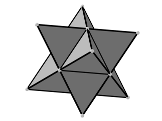
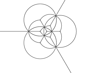
Figure 1. An equilateral surface of genus $0$, built from 24 equilateral triangles, and the corresponding triangulation of the Riemann sphere.

1.1 Question.

Which Riemann surfaces are equilaterally triangulable?

We emphasise that Question 1.1 concerns complex rather than metric structures. That is, a conformal isomorphism from a given Riemann surface $X$ to an equilateral surface $E$ induces a flat metric on $X$ having isolated cone singularities; different triangulations will lead to different metrics. Question 1.1 asks whether $X$ supports any such “equilateral triangulation”.

There are only countably many constellations in which one may glue finitely many triangles together. So there are only countably many compact equilateral surfaces, and hence most compact Riemann surfaces can not be equilaterally triangulated. The first explicit mention of equilateral triangulations on compact surfaces in the literature of which we are aware is in the context of string theory [BKKM86]. In response to [BKKM86], and making use of ideas from Grothendieck’s 1984 “Esquisse d’un programme” [Gro97] relating to work of Belyi [Bel79], Shabat and Voevodskii [VS89] point out that $X$ is equilaterally triangulable if and only if there exists a Belyi function $f\colon X\to\hat{\mathbb{C}}$; that is, a meromorphic function whose only critical values are $-1$, $1$ and $\infty$. Compare Proposition 2.7.

Such a surface is called a Belyi surface. Belyi’s theorem [Bel79, Theorem 4], see also [Bel02], states that $X$ is a Belyi surface if and only if $X$ is defined over a number field. (That is, $X$ can be represented as a smooth projective variety, defined by equations with algebraic coefficients.) In particular, this classical theorem gives a complete answer to Question 1.1 in the compact case. Belyi functions on compact surfaces are the subject of intense research, particularly in connection with Grothendieck’s programme for studying the absolute Galois group. Compare [Sch94, LZ04, JW16].

It seems natural to study Question 1.1 also for non-compact surfaces. See below for motivations of this problem from complex dynamics, in terms of the existence of finite-type maps, and from the point of view of conformal tilings. The answer is trivial in the case of the Euclidean or hyperbolic plane or the bi-infinite cylinder. Indeed, the plane can be tesselated using equilateral triangles; since this tesselation is periodic, it also provides a tesselation of the cylinder $\mathbb{C}/\mathbb{Z}$. Equilateral triangulations of the hyperbolic plane are provided by the classical hyperbolic triangle groups. Furthermore, it is not difficult to obtain equilaterally triangulated surfaces that are conformally equivalent to the three-punctured sphere or the once-punctured disc; see Section 2 and Figure 5.

Every Riemann surface $X$ is triangulable by Radó’s theorem [Rad25]. Replacing each element of the triangulation by an equilateral triangle, we see that there is an equilaterally triangulable surface topologically equivalent to $X$. However, in general the two surfaces are not conformally equivalent. Indeed, Riemann surfaces are arranged in moduli spaces, which are nontrivial real or complex manifolds except in the finitely many cases mentioned above. The simplest examples of non-trivial moduli spaces of non-compact surfaces are provided by round annuli $\{1<\lvert z\rvert<R\}$, which form a real one-dimensional family parameterised by $R\in(1,\infty)$, and four-punctured spheres, which are organised in a one-complex-dimensional moduli space, locally parameterised by the cross ratio of their punctures. As far as we are aware, Question 1.1 is open even for these two simple cases. We give a complete answer for all non-compact surfaces, which shows that this case differs fundamentally from that of compact Belyi surfaces.

1.2 Theorem.

Every non-compact Riemann surface is equilaterally triangulable.

As with compact surfaces, we can rephrase equilateral triangulability in terms of Belyi functions.

1.3 Definition.

Let $X$ be a (compact or non-compact) Riemann surface. A meromorphic function $f\colon X\to\hat{\mathbb{C}}$ is a Belyi function if $f$ is a branched covering whose branched points lie only over $-1$, $1$ and $\infty$.

Remark 1.

Here $f$ is called a branched covering if every point $w\in\hat{\mathbb{C}}$ has a simply connected neighborhood $U$ such that each connected component $V$ of $f^{-1}(U)$ is simply connected and $f\colon V\to U$ is a proper map topologically equivalent to $z\mapsto z^{d}$ for some $d\geq 1$.

Observe that, by definition of a branched covering $f\colon X\to\hat{\mathbb{C}}$, $X$ is the natural domain of $f$. That is, there is no Riemann surface $Y\supsetneq X$ such that $f$ extends to a holomorphic function $\tilde{f}$ on $Y$. Indeed, otherwise let $z$ belong to the relative boundary of $X$ in $Y$ and set $w\mathrel{\vbox{\hbox{\scriptsize.}\hbox{\scriptsize.}}}=\tilde{f}(z)$. If $U$ is a small neighbourhood of $w$, then there is a connected component $V$ of $f^{-1}(U)$ such that $f\colon V\to U$ is not onto, and in particular not proper.

Remark 2.

The Belyi functions $f\colon\mathbb{C}\to\hat{\mathbb{C}}$ are precisely the transcendental meromorphic functions with three critical values and no asymptotic values. See [Lan02] and [Ere04] for a discussion of the function-theoretic properties of these functions.

The following is an equivalent formulation of Theorem 1.2; see Proposition 2.7.

1.4 Theorem.

Every non-compact Riemann surface supports a Belyi function.

It is a consequence of the classical Riemann-Roch theorem that every compact Riemann surface is a branched cover of the Riemann sphere, branched over finitely many points. Hence Theorem 1.4 implies a new result for all Riemann surfaces.

1.5 Corollary.

Every Riemann surface is a branched cover of the sphere with only finitely many branched values.

Remark 1.

Gunning and Narasimhan [GN67] proved that every open Riemann surface $X$ admits a holomorphic immersion into the complex plane. That is, there exists a holomorphic mapping $f\colon X\to\mathbb{C}$ which is a local homeomorphism. However, this function cannot be a covering map if $X\neq\mathbb{C}$; so the inverse $f^{-1}$ necessarily has some, and potentially infinitely many, transcendental singularities in $\mathbb{C}$. In particular, such $f$ is not a branched covering.

Remark 2.

For a general compact Riemann surface $X$ of genus $g\geq 2$, the minimal number of branched values required in the theorem is $3g$. Indeed, the moduli space of $X$ has complex dimension $3g-3$. The subset consisting of those surfaces for which there is a branched cover branched over only $B\geq 3$ values is a countable union of submanifolds of dimension at most $B-3$. Thus, for a general surface $X$, the number of branched values in Corollary 1.5 is at least $B=3g$. On the other hand, if $X$ is any surface of genus $g$, and $P$ is a Weierstrass point of $X$, then there is a function $f\colon X\to\hat{\mathbb{C}}$ having a single pole at $P$ of degree at most $g$. By the Riemann-Hurwitz formula, $f$ has at most $3g-1$ finite critical values, and hence $3g$ critical values in total. (We thank Alex Eremenko for pointing out this argument.) For $g=1$, the moduli space is one-dimensional, so we need at least $B=4$ critical values in general; this is achieved by the Weierstrass $\wp$-function. On the other hand, Theorem 1.4 shows that $B=3$ always suffices for non-compact $X$.

Theorems 1.2 and 1.4 may seem surprising since the function $f$ is determined by an underlying equilateral triangulation, which is determined by an infinite graph on the surface, a discrete and non-flexible object. In contrast, Riemann surfaces are parameterised by complex manifolds, so the triangulation in Theorem 1.2 and the Belyi function $f$ in Theorem 1.4 cannot depend continuously on $X$ as it varies in a given moduli space. A similar phenomenon appears in the setting of circle packings: Every non-compact Riemann surface of finite conformal type (see Section 2) can be filled by a circle packing [Wil03]. Here a circle packing is a locally finite collection of circles whose tangency graph is a triangulation, and again this tangency graph completely determines the surface. However, despite the similarity of statements, the techniques used in [Wil03] have no obvious counterpart in the setting of equilateral surfaces. Indeed, [Wil03, Section 3] discusses how one may modify an existing partial packing to a full packing by replacing only one of the circles by another chain of circles. On the other hand, an equilateral triangulation is uniquely determined by any one of its triangles; see Remark 2.6.

There is a long history of constructing functions with finitely many singular values using quasiconformal mappings. See [Wit55] and [GO08, Chapter 7]; for a modern example, compare Bergweiler and Eremenko [BE19]. The control of the geometric behaviour of the resulting functions that can be achieved with classical methods is limited, but recently the first author introduced the conept of quasiconformal folding [Bis15]. This technique allows the very flexible construction of functions with finitely many singular values and prescribed behaviour. It has subsequently been used by authors including Fagella, Godillon and Jarque [FGJ15], Lazebnik [Laz17], Osborne and Sixsmith [OS16], and the second author [Rem16] to construct examples in transcendental dynamics on the plane. Compare Martí-Pete and Shishikura [MPS20] for a related construction that does not use quasiconformal folding.

While quasiconformal folding has been applied mostly to construct entire functions $f\colon\mathbb{C}\to\mathbb{C}$, it also allows the construction of meromorphic functions on more general Riemann surfaces. More precisely, given any Riemann surface $X$ (compact or not), quasiconformal folding allows one to construct a quasiregular map $f$ on $X$ that is branched only over $-1$, $1$ and $\infty$. Moreover, $f$ can be chosen to be “almost” holomorphic (more formally, its dilatation is bounded by a uniform constant and supported on a subset of $X$ of arbitrarily small area). It follows that there is a Belyi function on a surface $\tilde{X}$ close to $X$, establishing that equilaterally triangulable surfaces are dense in every moduli space; compare [Bis15, Section 15]. However, in general $\tilde{X}$ and $X$ have different complex structures.

Establishing Theorem 1.4 hence requires new ideas, which can be outlined as follows. We begin by subdividing $X$ into countably many pieces of finite topological type. We construct a finite triangulation on the first such piece $S$ that is almost equilateral; more precisely, it becomes equilateral after a quasiconformal change of the complex structure on $S$. By a careful analysis we see that this change can be kept so small that the new surface $\tilde{S}$ re-imbeds into $X$. This allows us to continue with our construction. An additional subtlety arises from the fact that choices made at earlier stages of the construction will influence how small we can keep our change in complex structure on subsequent pieces. It turns out that it is possible to control this influence by choosing the equilateral triangulation on each $S$ carefully, together with results on the area distortion under quasiconformal mappings.

The partial equilateral triangulations could be constructed by quasiconformal folding. Instead, we use a direct and more elementary method – though still motivated by the ideas of [Bis15] – which has the additional advantage that the number of triangles meeting at a single point is bounded by a universal constant. In particular, we obtain the following strengthening of Theorem 1.4.

1.6 Theorem.

There is a universal constant $D$ such that the Belyi function in Theorem 1.4 can be chosen to have local degree $\leq D$ at every point.

Our proof allows many choices at each stage of the inductive construction, and hence even shows the existence of uncountably many different Belyi functions on $X$. We thus obtain a new characterisation of compact Riemann surfaces.

1.7 Corollary.

A Riemann surface $X$ is compact if and only if supports at most countably many different Belyi functions, up to pre-composition by conformal automorphisms.

Finite-type maps

Let $X$ and $Y$ be Riemann surfaces, where $Y$ is compact. Following Epstein [Eps93], a holomorphic function $f\colon X\to Y$ is a finite-type map if there is a finite set $S$ such that

$$f\colon X\setminus f^{-1}(S)\to Y\setminus S$$

is a covering map, and furthermore $f$ has no removable singularities at any punctures of $X$. The smallest such set $S$ is called the set of singular values, and denoted by $S(f)$.

Epstein proved that finite-type maps have certain transcendence properties near the boundary, reminiscent of the Ahlfors five islands theorem [Eps93, Proposition 9]. In particular, he proved that, when $X\subset Y$, the fundamental results of the classical iteration theory of rational functions, and of entire/meromorphic functions with a finite set of singular values, remain valid for finite-type maps. Compare also [CE18] and [Rem09, Section 2].

It is a natural question for which pairs of $X$ and $Y$ finite-type maps exist. Corollary 1.5 shows that there are finite-type maps $X\to\hat{\mathbb{C}}$ for every Riemann surface $X$. In particular, when $X\subsetneq\hat{\mathbb{C}}$, we obtain the existence of many new non-trivial finite-type dynamical systems.

It is also possible to prove the existence of finite-type maps $f\colon X\to T$ with $\#S(f)=1$ for every non-compact Riemann surface $X$ and every torus $T$. This is achieved by a modification of our methods that leads to the existence of a Shabat function on $X$; i.e. a branched covering map from $X$ to the complex plane $\mathbb{C}$ which is branched only over two values. Postcomposing the Shabat function with a projection to the torus that identifies the two critical values yields the desired finite-type map. The details of the construction will be given in a subsequent article.

The question of the existence of finite-type maps with target $Y$ becomes more subtle when $Y$ is hyperbolic. By Liouville’s theorem, $X$ must be hyperbolic if such a map is going to exist. In fact, it is possible to show that the boundary of $X$ must be uniformly perfect. That is, the hyperbolic length of any non-contractible closed curve in $X$ is bounded uniformly from below.

In [Bis15, Section 16], the first author uses quasiconformal folding to construct finite-type maps from certain finite Riemann surfaces $U$ (see Section 2) to all compact hyperbolic surfaces. This is achieved by constructing a branched covering $U\to\mathbb{D}$ with only two branched points in $\mathbb{D}$, and postcomposing with the universal covering map. If $U^{\prime}$ is any finite Riemann surface, then a refinement of the method of [Bis15, Section 16] shows that $U$ can be chosen arbitrarily close to $U^{\prime}$ in its moduli space. In particular, if $U^{\prime}$ is a subpiece of some compact Riemann surface $Y$, bounded by disjoint analytic boundary circles, then the perturbed surface $U$ is also embeddable in $Y$ (see Proposition 4.1 below), and we obtain new examples of finite-type dynamical systems with hyperbolic target $Y$. The following appears plausible in view of our results.

1.8 Conjecture.

On every finite Riemann surface $U$, there is a branched covering $f\colon U\to\mathbb{D}$ branched over at most two points. In particular, if $Y$ is any compact hyperbolic surface, and $\pi\colon\mathbb{D}\to Y$ is its universal cover, then $\pi\circ f\colon U\to Y$ is a finite-type map.

The method of [Bis15, Section 16] can also be used to construct finite type maps to hyperbolic surfaces on some infinitely-connected $U$. It is an interesting question whether such functions exist on all hyperbolic surfaces with uniformly perfect boundary.

Conformal tilings

Bowers and Stephenson [BS97, BS17, BS19] study conformal tilings of a Riemann surface $X$, which are obtained by allowing general regular polygons, of the same fixed side-length, in our construction above. In particular, every equilateral triangulation of $X$ is also a conformal tiling. Conversely, the barycentric subdivision of a conformal tiling is an equilateral triangulation, so a tiling exists if and only if the surface is equilaterally triangulable.

Bowers and Stephenson are mainly interested in the case where $X$ is simply connected. As mentioned above, these surfaces are equilaterally triangulable for elementary reasons; the cited articles exhibit many interesting and beautiful different such conformal tilings. However, [BS17, Appendix B] also raises the question which multiply-connected surfaces admit conformal tilings; this is equivalent to Question 1.1, and Theorem 1.2 (together with Belyi’s theorem for the compact case) gives a complete answer.

Random equilateral triangulations

There is an extensive literature on random equilateral triangulations of compact surfaces; see e.g. [BM04, Mir13, BCP19]. In statistical physics, there has been intensive study of the metric and conformal structures on compact surfaces built from random equilateral triangulations, quadrangulations or more general random maps, and especially of the limits of these random surfaces when the number of triangles tends to infinity but the genus is held constant. For example, a recent major result of Miller and Sheffield [MS20, MS16a, MS16b] shows that two such limiting objects – “Liouville quantum gravity” and the “Brownian map” – are essentially the same. Compare also [LG07, LG19, Mie14]. For analogous constructions on higher genus compact surfaces, see e.g. [DR15, BM17].

In all of these cases, the distribution of the conformal structures of the discrete random surfaces is supported on a countable set in moduli space (Belyi surfaces in the case of random equilateral triangulations), but for a fixed genus, the distributions conjecturally converge to continuous distributions. What can be said about random non-compact triangulations? For the Euclidean plane, this question has been addressed by Angel and Schramm [AS03]: they show how to define a probability measure on the metric space of rooted planar triangulations, called a uniform infinite planar triangulation (UIPT). Hyperbolic versions have also been considered; compare [AR15, Cur16, Bud20].

The UIPT can be thought of as a uniformly random surface with the topology of a plane. Can one also make sense of the notion of a uniformly random surface with the topology of a cylinder, or some other non-compact topology, such as a compact surface with a puncture? Scott Sheffield suggested the following formulation of this problem. Begin with the UIPT, which comes with a distinguished ”origin” triangle, and then cut out that origin triangle and glue in some finite genus graph. By our results, it is at least possible that there is a continuous limiting distribution. Do all conformal structures occur if we glue in a random finite genus graph? Does a neighborhood of a point in moduli space occur if we glue in a fixed choice?

Basic notation

The symbols $\mathbb{C}$ and $\hat{\mathbb{C}}$ denote the complex plane and Riemann sphere, respectively. The (Euclidean) disc of radius $\rho$ around $w\in\mathbb{C}$ is denoted by $D(w,\rho)$; the unit disc is denoted $\mathbb{D}\mathrel{\vbox{\hbox{\scriptsize.}\hbox{\scriptsize.}}}=D(0,1)$. In a slight abuse of terminology, we also denote the complement of the closed unit disc by $D(\infty,1)=\hat{\mathbb{C}}\setminus\overline{\mathbb{D}}$. For $R>1$ we define the following annuli (see Figure 3):

$$\mathbb{A}(R)\mathrel{\vbox{\hbox{\scriptsize.}\hbox{\scriptsize.}}}=\{1/R<\lvert z\rvert<R\};$$

$$\mathbb{A}_{-}(R)\mathrel{\vbox{\hbox{\scriptsize.}\hbox{\scriptsize.}}}=\{1/R<\lvert z\rvert<1\}=\mathbb{A}(R)\cap\mathbb{D};\quad\text{and}$$

$$\mathbb{A}_{+}(R)\mathrel{\vbox{\hbox{\scriptsize.}\hbox{\scriptsize.}}}=\{1<\lvert z\rvert<R\}=\mathbb{A}(R)\setminus\overline{\mathbb{D}}.$$

We assume throughout that the reader is familiar with the theory of Riemann surfaces and quasiconformal mappings, and refer e.g. to [For91, LV73, Hub06] for reference. In addition, the proofs in Section 4 use background from Teichmüller theory. However, this technique is not required to understand the statements of the main results in these sections, or their applications in the proofs of our main theorems.

Acknowledgements

This research arose from an interesting and stimulating e-mail discussion concerning finite-type maps with Adam Epstein and Alex Eremenko; we thank them both for the initial inspiration and subsequent helpful comments and conversations on this work. We are grateful to J. Martel [Mar13] for pointing out the result of Williams on circle packing, Curt McMullen for helpful comments on the case of compact surfaces, and Daniel Meyer for highlighting the connection with conformal tilings. We thank Dmitry Chelkak and Scott Sheffield for providing helpful comments and references on random triangulations.

2. Riemann surfaces, triangulations and Belyi functions

In this section, we collect background on Riemann surfaces and triangulations. In particular, we recall the proof of the fact that a Riemann surface is equilaterally triangulable if and only if it supports a Belyi function.

Riemann surfaces and conformal metrics

A Riemann surface $X$ is a connected one-dimensional complex Hausdorff manifold. By a conformal metric on a Riemann surface we mean a length element that takes the form ${\rm d}s=\rho(z)\lvert{\rm d}z\rvert$ in local coordinates (where $\rho$ is a continuous positive-valued function). Note that each conformal metric gives rise to an area element, $\rho^{2}(z)\lvert{\rm d}z\rvert^{2}$. When such a metric $\rho$ is given, we shall write $\operatorname{dist}_{\rho}$ for the corresponding distance function; i.e. $\operatorname{dist}_{\rho}(z,w)$ is the largest lower bound for the $\rho$-length of a curve connecting $z$ and $w$. (We omit the subscript $\rho$ when it is clear from the context which metric $\rho$ is to be used.)

By the uniformisation theorem, every Riemann surface can be endowed with a conformal metric of constant curvature; in the case of positive or negative curvature, this metric becomes unique by requiring that the curvature is $1$ or $-1$, respectively. We emphasise that we use conformal metrics only in an inessential way, to provide a measure of “smallness” of area on compact pieces of a Riemann surface. Any two conformal metrics on a compact surface (or surface-with-boundary) are equivalent; indeed, the quotient of their densities is a continuous function and hence assumes a positive and finite maximum and minimum. Thus the precise choice of metric will be irrelevant.

Finite pieces of Riemann surfaces

A Riemann surface $X$ is said to be finite if it is of finite genus with a finite number of boundary components, none of which are degenerate. In other words, $X$ is conformally equivalent to a compact Riemann surface with at most finitely many topological discs removed. This notion should not be confused with that of finite type: A surface has finite topological type if it is homeomorphic to a compact surface with finitely many points removed, and finite conformal type if this homeomorphism can be chosen analytic. In particular, a non-compact finite Riemann surface has finite topological type, but is never of finite conformal type. (See Figure 2.) To avoid ambiguities, we do not use the notion of finite conformal type in the remainder of the article.

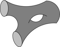
(a) Finite Riemann surface

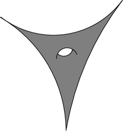
(b) Finite conformal type

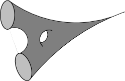
(c) Finite topological type

Figure 2. Three different notions of finiteness of Riemann surfaces.

In our context, finite Riemann surfaces often arise as subsets of a larger surface $X$. The following notation will be convenient.

2.1 Definition (Finite pieces).

Let $X$ be a Riemann surface, and let $U\subsetneq X$ be a finite Riemann surface. If $U$ is pre-compact in $X$, then we say that $U$ is a finite piece of $X$. If furthermore $\partial U\subset X$ consists of finitely many analytic Jordan curves (called the boundary curves of $U$), then $U$ is said to be analytically bounded.

Boundary coordinates and hemmed surfaces

We shall construct triangulations on finite pieces of our Riemann surface $X$. To be able to combine such partial triangulations, we also need to record, for a finite piece, suitable parameterisations of its boundary. We hence introduce the following notion. (See Figure 3.)

2.2 Definition.

A hemmed Riemann surface is a non-compact finite Riemann surface $U$, together with analytic parameterisations of its boundary curves. More precisely, let $\Gamma$ be the set of boundary curves of $U$ (or, in other words, the set of ends of $U$). For each $\gamma\in\Gamma$, let

$$\varphi^{\gamma}\colon\mathbb{A}_{-}(\mathbb{R}^{\gamma})\to A^{\gamma},$$

where $R^{\gamma}>1$, be a conformal map to an annulus $A^{\gamma}\subset U$ such that $\varphi^{\gamma}(z)\to\gamma$ as $\lvert z\rvert\to 1$. We furthermore assume that the image annuli $A^{\gamma}$ have pairwise disjoint closures. Then we say that $U$ is a hemmed Riemann surface with boundary coordinates $(\varphi^{\gamma})_{\gamma\in\Gamma}$.

Observe that the closure of every hemmed Riemann surface is a compact Riemann surface-with-boundary, with charts on the boundary curve $\gamma$ given by $(\varphi^{\gamma})^{-1}$. Conversely, any compact Riemann surface-with-boundary can be given the structure of a hemmed Riemann surface by choosing an annulus $A^{\gamma}$ around each boundary curve, and letting $\varphi^{\gamma}$ be a conformal map from a round annulus to $A^{\gamma}$. Different choices of annuli will lead to different boundary coordinates, and hence to different “hemmed surfaces”.

Figure 3. The annuli $\mathbb{A}_{+}(R)$ and $\mathbb{A}_{-}(R)$ (left), and a hemmed Riemann surface (right)

Triangulations

2.3 Definition.

Let $X$ be a Riemann surface, or a Riemann surface-with-boundary. A triangulation of $X$ is a countable and locally finite collection of closed topological triangles that cover $X$, such that two triangles intersect only in a full edge or in a vertex.

In other words, a triangulation furnishes $X$ with the structure of a locally finite simplicial complex. By a theorem of Radó from 1925 [Rad25] (see [For91, §23] or [Hub06, Theorem 1.3.3]), every Riemann surface is second countable, and hence triangulable.

Let $\mathcal{T}$ be a triangulation and let $\Delta$ be the Euclidean equilateral triangle inscribed in the unit circle, with a vertex at $1$. For each topological triangle $T\in\mathcal{T}$, let $\varphi_{T}$ denote a biholomorphic isomorphism that takes $T$ to $\Delta$, mapping vertices to vertices. Observe that $\varphi_{T}$ is unique up to postcomposition by a rotational symmetry of $\Delta$.

2.4 Definition.

The triangulation $\mathcal{T}$ is equilateral if, on every edge $e$ with two adjacent triangles $T$ and $\tilde{T}$, the maps $\varphi_{T}$ and $\varphi_{\tilde{T}}$ agree up to a reflection symmetry of $\Delta$. If such a triangulation exists, we say that $X$ is equilaterally triangulable.

It is elementary to see that this agrees with the definition given in the introduction, with one caveat: The “triangulations” mentioned there allowed two triangles to intersect in more than one edge; let us call these generalised triangulations in the following. Given an equilateral generalised triangulation, we can perform a barycentric subdivision of all triangles, inserting a new vertex in the barycenter of each face and the mid-point of each edge. In this triangulation, no two triangles intersect in more than one edge. The following observation shows that this triangulation is also equilateral; see Figures 4 and 5(c). Compare [BS17, §1.3].

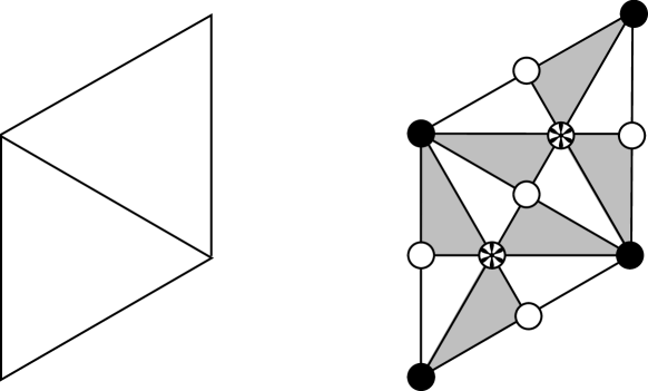
Figure 4. Any equilateral triangulation can be refined by barycentric subdivision into a new equilateral triangulation that is bipartite and 3-coloured, as described after the proof of Proposition 2.7.

2.5 Lemma (Equilateral triangulations and reflections).

A generalised triangulation of $X$ is equilateral if and only if the two triangles adjacent to a given edge are related by reflection. That is, suppose that the triangles $T$ and $\tilde{T}$ are both adjacent to an edge $e$. Then there exists an antiholomorphic homeomorphism $\iota\colon T\to\tilde{T}$ that fixes $e$ pointwise and maps the third vertex of $T$ to the corresponding vertex of $\tilde{T}$.

Proof.

Let $e$, $T$ and $\tilde{T}$ be as in the statement, and let $\varphi_{T}$ and $\varphi_{\tilde{T}}$ be as defined above. Suppose that $\varphi_{\tilde{T}}|_{e}=R\circ\varphi_{T}|_{e}$, where $R$ is a reflection symmetry of $\Delta$. Then

$$\iota\mathrel{\vbox{\hbox{\scriptsize.}\hbox{\scriptsize.}}}=\varphi_{\tilde{T}}^{-1}\circ R\circ\varphi_{T}$$

is an antiholomorphic bijection as in the statement of the observation.

Conversely, suppose $\iota$ is such a bijection. Then $R\mathrel{\vbox{\hbox{\scriptsize.}\hbox{\scriptsize.}}}=\varphi_{\tilde{T}}\circ\iota\circ\varphi_{T}^{-1}$ is an antiholomorphic automorphism of the triangle $\Delta$, mapping vertices to vertices. Thus $R$ is a reflection symmetry of $\Delta$, as required. ∎

2.6 Remark.

It follows from the Schwarz reflection principle that, if a “reflection” $\iota\colon T\to\tilde{T}$ as above exists, then $\iota$ and hence $\tilde{T}$ are uniquely determined by $T$. In particular, an equilateral triangulation $\mathcal{T}$ is uniquely determined by any given triangle $T\in\mathcal{T}$.

The equivalence of Theorems 1.2 and 1.4 is a consequence of the following fact.

2.7 Proposition (Triangulations and Belyi functions).

A Riemann surface $X$ is equilaterally triangulable if and only if there is a Belyi function on $X$.

Proof.

Proposition 2.7 is well-known in the compact case; see [VS89], and the proof in the general case is the same [BS17, §1.3]. For the reader’s convenience, we present it briefly. First suppose that $f\colon X\to\hat{\mathbb{C}}$ is a Belyi function. Consider the generalised triangulation of the sphere into two triangles corresponding to the upper and lower half-plane, with vertices at $1$, $-1$ and $\infty$. By the Schwarz reflection principle and Observation 2.5, this triangulation is equilateral. Since the critical values of $f$ are at the vertices of the triangulation, we may lift it to $X$, to obtain a generalised equilateral triangulation. As discussed above, a barycentric subdivision leads to a triangulation in the stricter sense, and the proof of the “if” direction is complete.

Now suppose that an equilateral triangulation of the surface $X$ is given. Let $\mathcal{T}$ be the corresponding collection of topological triangles, with conformal maps $\varphi_{T}\colon T\to\Delta$ for $T\in\mathcal{T}$, as above. Let $\psi\colon\Delta\to\mathbb{D}$ be the conformal isomorphism that fixes $0$ and $1$, and consider the function

$$f\colon X\to\hat{\mathbb{C}};\colon z\mapsto F_{3}(\psi(\varphi_{T}(z)))\qquad(z\in T),$$

where $F_{3}$ is the degree $6$ rational map

$$F_{3}(z):=\frac{1}{2}(z^{3}+z^{-3}).$$

Let $\rho$ denote rotation by 60° around $0$, and let $\sigma$ denote complex conjugation. Observe that $\psi$ commutes with both operations, and that $F_{3}\circ\rho=F_{3}\circ\sigma=F_{3}$ on $\partial\mathbb{D}$. The group of symmetries of $\Delta$ is generated by $\rho$ and $\sigma$, and thus $f$ is indeed a well-defined holomorphic function on $X$. Clearly $f$ is a branched covering with no critical values outside of $-1$, $1$ and $\infty$; so $f$ is a Belyi function. ∎

2.8 Remark.

The generalised equilateral triangulation obtained from the Belyi function $f$ in the above proof is 3-colourable: Its vertices may be coloured with the three colours $\{-1,1,\infty\}$ in such a way that adjacent vertices have different colours. Conversely, suppose $\mathcal{T}$ is a generalised equilateral triangulation together with a 3-colouring of its vertices; let us call this a 3-coloured triangulation. Then the three vertices of any triangle $T\in\mathcal{T}$ may be coloured with the three different colours $-1$, $1$ and $\infty$, and we may map $T$ conformally to either the upper or lower half-plane in such a way that each vertex corresponds to the point indicated by its colour. By Schwarz reflection the collection of these conformal maps extends to a Belyi function on $X$. Hence the Belyi functions on $X$ are in one-to-one correspondence with the 3-coloured generalised equilateral triangulations on $X$.

Not every equilateral triangulation $\mathcal{T}$ (generalised or otherwise) can be 3-coloured; consider, for example, the triangulation of the sphere into four congruent spherical equilateral triangles. However, the barycentric subdivision of $\mathcal{T}$ is always $3$-colourable; indeed, we may mark the original vertices with the colour $1$, the new vertices added on existing edges with the colour $-1$, and the vertices added in each face with $\infty$ (Figure 4). This yields precisely the triangulation corresponding to the Belyi function in the “only if” direction of Proposition 2.7.

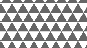
(a) The complex plane $\mathbb{C}$

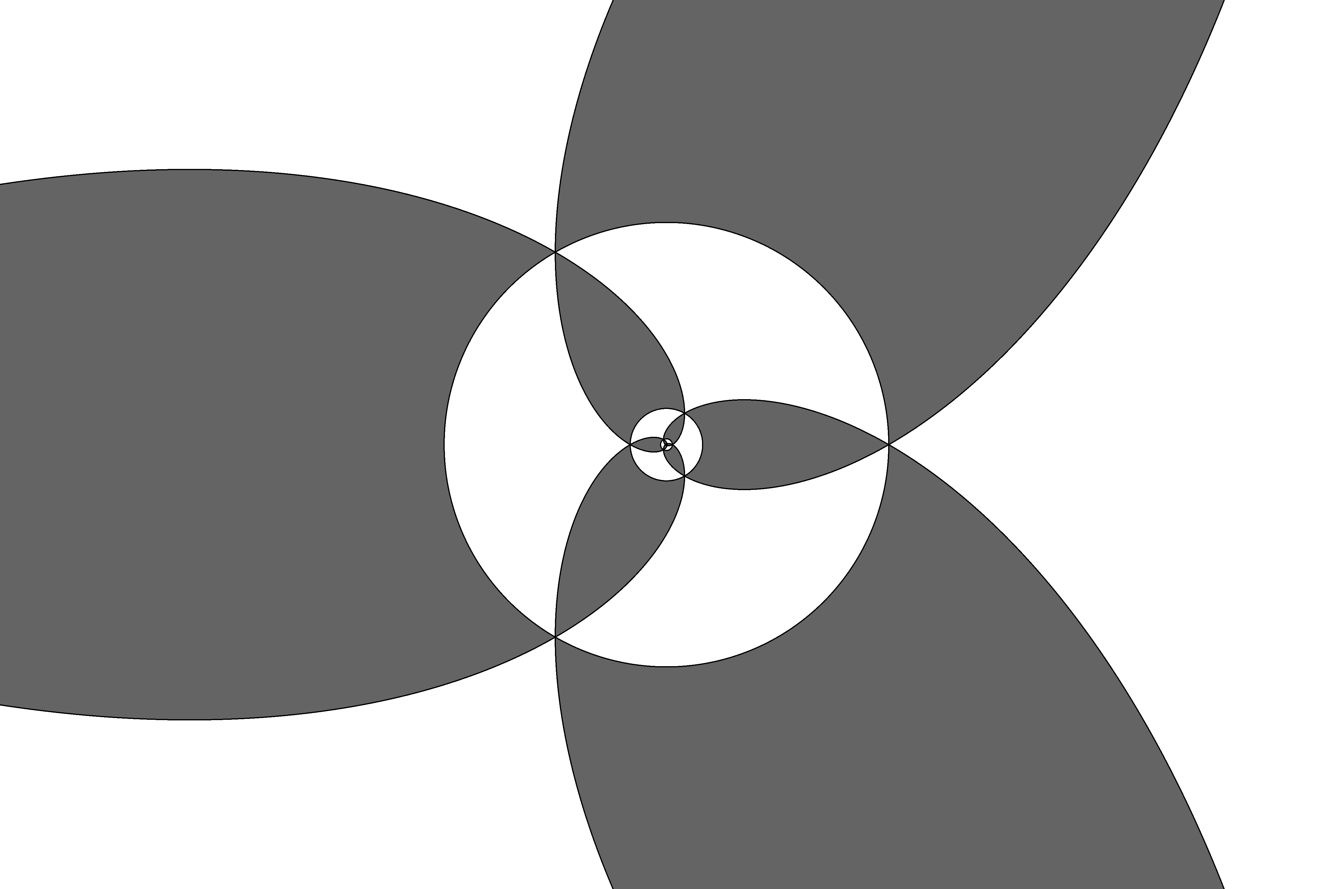
(b) The punctured plane $\mathbb{C}^{*}$

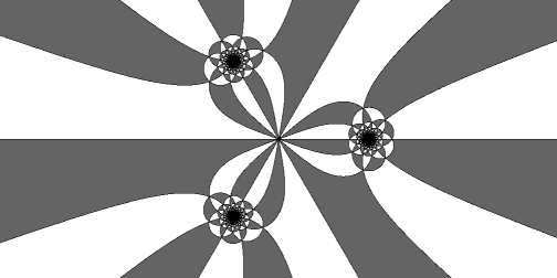
(c) The three-punctured sphere

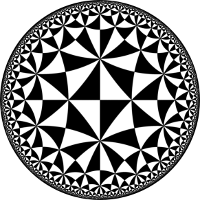
(d) The unit disc $\mathbb{D}$

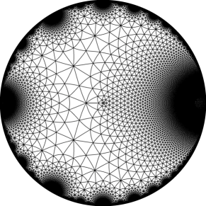
(e) The punctured disc $\mathbb{D}^{*}$

Figure 5. Equilateral triangulations of non-compact Riemann surfaces with trivial moduli spaces.

Elementary cases of Theorem 1.2

The triangular lattice, which tesselates the plane into equilateral triangles, provides an equilateral triangulation of both the plane and the bi-infinite cylinder; i.e., the punctured plane. This triangulation is $3$-colourable; the corresponding Belyi function is elliptic, and can be described as the universal orbifold covering map of the sphere with signature $(3,3,3)$; see [Mil06, Appendix E].

The unit disc $\mathbb{D}$ is equilaterally triangulated by the classical hyperbolic triangle groups. We may obtain an equilateral triangulation of the punctured disc $\mathbb{D}^{*}=\mathbb{D}\setminus\{0\}$ as follows. The Klein $j$-invariant $j\colon\mathbb{H}^{+}\to\mathbb{C}$ is a branched covering map from the upper half-plane $\mathbb{H}^{+}$ to the complex plane which is invariant under the modular group and has only two branched values, which we may arrange to be $0$ and $1$. In particular, $j(\zeta+1)=j(\zeta)$ for all $z\in\mathbb{H}^{+}$, and hence $J\colon\mathbb{D}^{*}\to\mathbb{C};z\mapsto j(\log z/(2\pi i))$ is a well-defined branched covering map with branched values $0$ and $1$. Let $\mathcal{T}$ be a triangulation of the complex plane for which $0$ and $1$ are vertices (for example, the triangular lattice $\mathcal{T}_{\operatorname{eucl}}$ discussed above, chosen such that $[0,1]$ is the edge of one of the triangles). Then the preimage of $\mathcal{T}$ under $J$ is an equilateral triangulation of $\mathbb{D}^{*}$; see Figure 5(e).

A similar construction leads to triangulations of multiply-punctured spheres. Note that

$$g\colon\hat{\mathbb{C}}\to\hat{\mathbb{C}};\quad z\mapsto\frac{z^{n}}{z^{n}-1}$$

is a degree $n$ branched covering of the sphere, branched over $0$ and $1$. The preimage under $g$ of an equilateral triangulation $\mathcal{T}$ of $\hat{\mathbb{C}}\setminus\{1\}$ (for example, the image of the triangular lattice under $z\mapsto(z+1)/z$) is an equilateral triangulation of the sphere punctured at the $n$-th roots of unity; see Figure 5(c).

In particular, the thrice-punctured sphere is equilaterally triangulable, and there exist equilaterally triangulable $n$-punctured spheres for all $n$. However, for $n>3$, we have equilaterally triangulated only one specific member of the moduli space of $n$-punctured spheres, which has positive dimension. We may obtain others by modifying the construction, e.g. by using different degree $d$ covering maps whose critical values lie in the triangular lattice. Nonetheless, this yields at most countably many different surfaces among the uncountably many possible choices.

3. Triangulations of hemmed Riemann surfaces

Let $X$ be a hemmed Riemann surface, in the sense of Definition 2.2. Our goal in this section is to show that there is a triangulation of $X$ that is close to an equilateral triangulation, in a quasiconformal sense. Moreover, in boundary coordinates, the triangulation will simply subdivide each boundary circle $\gamma$ into a large number $d^{\gamma}$ of equal arcs, where the $d^{\gamma}$ can be chosen independently of each other as long as they are sufficiently large. This will later allow us to glue together triangulations of different finite pieces of a given Riemann surface $X$.

To make this statement precise, we use the following notion.

3.1 Definition.

Let $d\geq 1$, and let

$$\Xi_{d}\mathrel{\vbox{\hbox{\scriptsize.}\hbox{\scriptsize.}}}=\{e^{2\pi ij/d}\colon j\in\mathbb{Z}\}$$

denote the set of all $d$-th roots of unity. We call $\Xi_{d}$ the standard partition of $S^{1}$ of size $d$; the intervals of $S^{1}\setminus\Xi_{d}$ are called the edges of the partition.

3.2 Proposition (Triangulations on hemmed Riemann surfaces).

There are $K_{0}>1$, $d_{0}\geq 6$ and a function $\Delta\colon(1,\infty)\to\mathbb{N}$, with the following property.

Let $U$ be a hemmed Riemann surface with boundary coordinates

$$\varphi^{\gamma}\colon\mathbb{A}^{-}(R^{\gamma})\to A^{\gamma}.$$

Denote the set of all boundary curves by $\Gamma$, and let $\rho$ be a conformal metric on $U$. Fix $d^{\gamma}\geq\Delta(R^{\gamma})$ for each $\gamma\in\Gamma$, and let $\eta>0$.

Then there is a homeomorphism $g$ from $\overline{U}$ to a finite equilateral surface-with-boundary $E$ such that the following hold.

1. Every vertex of $E$ is incident to at most $d_{0}$ edges.

2. For $\gamma\in\Gamma$, the map $g\circ\varphi^{\gamma}\colon S^{1}\to g(\gamma)$ maps each edge of $\Xi_{d^{\gamma}}$ to a boundary edge of $E$ in length-respecting fashion.

3. $g$ is $K_{0}$-quasiconformal on $U$.

4. The dilatation of $g$ is supported on the union $\bigcup_{\gamma}A^{\gamma}$, together with a set that has measure at most $\eta$ with respect to the metric $\rho$.

Remark 1.

A map respects length if it changes distances by a constant factor [Bis15, §4]. Note that the equilateral surface $E$ comes equipped with a natural distance inherited from its representation by equilateral triangles; this is a flat conformal metric, except possibly for cone singularities at the vertices of the triangulation.

We may rephrase b more explicitly as follows. Let $e$ be an edge of $\Xi_{d^{\gamma}}$. Then $g(\varphi^{\gamma}(e))$ is a boundary edge of $E$; let $T$ be the unique adjacent face. By the definition of an equilateral surface, $T$ is a copy of a planar equilateral triangle; in these coordinates, $g\circ\varphi^{\gamma}\circ\exp$, restricted to a component of $\log e$, is required to be the restriction of a complex affine map.

Remark 2.

It is crucial that the number $d_{\gamma}$ can be chosen arbitrarily large on each boundary curve $\gamma$, independently of the choice for the others.

The idea of the proof of Proposition 3.2 can be summarised as follows.

1. By cutting along finitely many essential curves, we may assume that $U$ has genus $0$, and hence is a subset of the plane.

2. We cover the complement of the annuli $A^{\gamma}$ in $U$ with small Euclidean equilateral triangles arranged in a triangular lattice.

3. We are left with finitely many annuli, one in each $A^{\gamma}$, between $\gamma$ and a curve consisting of edges taken from the above lattice. We interpolate between the partitions of these two boundaries by a triangulation that has bounded geometry, and hence is quasiconformally equivalent to an equilateral triangulation.

For the final step, we use an elementary statement concerning triangulations of rectangles.

3.3 Definition (Bounded-geometry partition of a rectangle boundary).

Let $R$ be a Euclidean rectangle. By a boundary partition of $R$ we mean a finite set $P$ of points on $\partial R$ that includes the four vertices of $R$ (i.e., a union of partitions of the four sides of $\partial R$). The edges of the partition are the connected components of $\partial R\setminus P$; two edges are adjacent if they have a common endpoint.

We say that the boundary partition $P$ has bounded geometry with constant $\lambda>1$ if

1. the lengths of adjacent edges differ by at most a factor of $\lambda$, and

2. all edges have length at most $\lambda\ell$, where $\ell$ is the length of the two shorter sides of $R$.

3.4 Proposition (Triangulations of a rectangle).

Let $\lambda>0$. Then there is a constant $\vartheta_{0}>0$ with the following property. If $Q$ is a rectangle and $P$ is a bounded-geometry boundary partition with constant $\lambda$, then there is a triangulation $T$ of the closed rectangle $Q$ into finitely many Euclidean triangles such that

1. all angles in all triangles in $T$ are bounded below by $\vartheta_{0}$;

2. the vertices of $T$ on $\partial Q$ are precisely the elements of $P$.

Since we are not aware of a reference, we give a proof of Proposition 3.4 in an appendix (Section 6.) We remark that the result can also be obtained using the (much more general) methods used in [Bis10].

Proof of Proposition 3.2.

Set $\Delta(R)\mathrel{\vbox{\hbox{\scriptsize.}\hbox{\scriptsize.}}}=1/\log R$. As mentioned in I, we prove the proposition first when $U$ has genus $0$. In this case, it turns out that the dilatation is supported only on the annuli $A^{\gamma}$, so we can take $\eta=0$.

For each $\gamma\in\Gamma$, glue a copy $D^{\gamma}$ of the closed disc $\overline{D(\infty,1)}=\hat{\mathbb{C}}\setminus\mathbb{D}$ into the surface $U$ at $\gamma$. More precisely, we obtain a Riemann surface structure on $U\cup\bigcup_{\gamma}D^{\gamma}$ by using the original charts of $U$, and adding the charts (with values in $\hat{\mathbb{C}}$)

$$z\mapsto\begin{cases}z&\text{if }z\in D^{\gamma}\\ (\varphi^{\gamma})^{-1}(z)&\text{if }z\in A^{\gamma}\end{cases}$$

on $D^{\gamma}\cup A^{\gamma}$. (For simplicity of notation, we use $z$ to denote both the point of $D^{\gamma}$ and the one of $\overline{D(\infty,1)}$ that it represents.)

The result is a compact Riemann surface of genus $0$, and hence conformally equivalent to the Riemann sphere $\hat{\mathbb{C}}$. In other words, we are now in the following situation:

$$U=\hat{\mathbb{C}}\setminus\bigcup_{\gamma\in\Gamma}\Phi^{\gamma}(\overline{\mathbb{D}})$$

is an analytically bounded surface, bounded by the curves $\gamma=\Phi^{\gamma}(S^{1})$. Here each $\Phi^{\gamma}$ is a conformal map defined on the disc $D(0,R^{\gamma})$, and the images of these functions have disjoint closures. Note that $\Phi^{\gamma}(z)=\varphi^{\gamma}(1/z)$ on $\mathcal{A}^{+}(R^{\gamma})$. We may choose coordinates on the sphere such that $\Phi^{\gamma}(0)=\infty$ for some $\gamma$, so that $\overline{U}\subset\mathbb{C}$. Let

$$\tilde{\gamma}\mathrel{\vbox{\hbox{\scriptsize.}\hbox{\scriptsize.}}}=\Phi^{\gamma}(\partial(D(0,\sqrt{R^{\gamma}})))$$

denote the core curve of the annulus $A^{\gamma}$, and let $\tilde{U}$ denote the subset of $U$ bounded by the curves $\tilde{\gamma}$. (In Figure 6, $\tilde{U}$ is the union of the light grey annulus and the white region.)

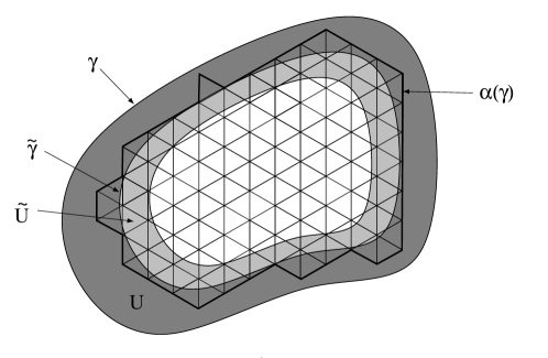
Figure 6. Definition of $\alpha(\gamma)$. For simplicity, the figure is drawn when $U$ is simply connected, with a single boundary curve $\gamma$.

For any $\varepsilon>0$, let $\mathcal{L}=\mathcal{L}_{\varepsilon}$ be a tiling of the plane by equilateral triangles of side-length $\varepsilon$. Let $\tilde{E}$ be the union of all triangles of $\mathcal{L}$ that intersect $\tilde{U}$. Since the curves $\tilde{\gamma}$ are smooth, for small $\varepsilon$ the domain $\tilde{E}$ is a finite equilateral Riemann-surface with boundary, with one boundary curve $\alpha(\gamma)$ contained in each $A^{\gamma}$ and homotopic to $\gamma$. See Figure 6. Note that $\tilde{E}$ and the remainder of the construction depend on $\varepsilon$; we suppress this dependence for simplicity of notation.

Set

$$\Sigma_{+}\mathrel{\vbox{\hbox{\scriptsize.}\hbox{\scriptsize.}}}=\exp^{-1}((\Phi^{\gamma})^{-1}(\alpha(\gamma)));$$

see Figure 7. Let $V_{+}$ and $E_{+}$ denote the sets of vertices and edges of $\Sigma_{+}$; that is, the preimages of the vertices and edges of the polygonal curve $\alpha(\gamma)$ under $\Phi^{\gamma}\circ\exp$. Also let $\Sigma_{-}$ denote the imaginary axis, and let $S$ denote the domain bounded by $\Sigma_{-}$ on the left and $\Sigma_{+}$ on the right. So $\Phi^{\gamma}\circ\exp$ maps the strip $S_{\gamma}$ to the annulus bounded by $\alpha(\gamma)$ and $\gamma$ as a universal covering map. Also define the strip

$$\tilde{S}\mathrel{\vbox{\hbox{\scriptsize.}\hbox{\scriptsize.}}}=\{x+iy\colon 0<x<\rho\mathrel{\vbox{\hbox{\scriptsize.}\hbox{\scriptsize.}}}=(\log R^{\gamma})/2\},$$

and let $\tilde{\Sigma}_{+}=\rho+i\mathbb{R}$ be its right boundary. Note that $\Phi^{\gamma}(\exp(\tilde{S}))$ is bounded by $\gamma$ and $\tilde{\gamma}$, and in particular $S\subset\tilde{S}$.

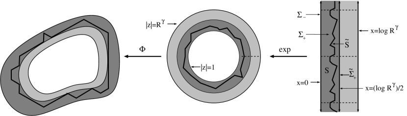
Figure 7. The definition of the strips $S$ and $\tilde{S}$.

Claim.

There are universal $K_{1}>1$ and $\lambda>1$ with the following property. If $\varepsilon>0$ is chosen sufficiently small in the definition of $\mathcal{L}$, then there is a $K_{1}$-quasiconformal homeomorphism

$$\Psi=\Psi^{\gamma}\colon S\to\tilde{S}$$

such that:

1. $\Psi(z+2\pi i)=\psi(z)+2\pi i$ for all $z$;

2. $\Psi(z)=z$ for $z\in\Sigma_{-}$;

3. $\Psi(V_{+})$ contains $\rho$;

4. the length of the intervals in $\tilde{E}_{+}\mathrel{\vbox{\hbox{\scriptsize.}\hbox{\scriptsize.}}}=\{\Psi(e)\colon e\in E_{+}\}$ is bounded above by $\rho$;

5. the lengths of adjacent intervals in $\tilde{E}_{+}$ differ at most by a factor of $\lambda$;

6. Let $e\in E_{+}$ and $\tilde{e}\mathrel{\vbox{\hbox{\scriptsize.}\hbox{\scriptsize.}}}=\Psi(e)$. Then $\Phi^{\gamma}\circ\exp\circ\Psi^{-1}$ respects length when restricted to $\tilde{e}$.

Proof of the claim.

The claim can be proved using the methods of [Bis15, Sections 3–4]. Instead, we sketch a direct argument. If $\varepsilon$ is sufficiently small, then by Koebe’s theorem, the edges of $\Sigma_{+}$ are very close to straight line segments. Moreover, the difference in angle between the edges of $\alpha(\gamma)$ and $\tilde{\gamma}$ is bounded away from $\pi/2$ (again, for small $\varepsilon$).

Indeed, if $\varepsilon$ is small enough, then $\tilde{\gamma}$ is nearly a straight line segment near each triangle. An edge of $\alpha(\gamma)$ cannot be the side of a triangle $T$ that has two vertices in $\tilde{U}$; in that case all three sides hit $\tilde{U}$ and so all three adjacent triangles also hit $\tilde{U}$. Therefore either no vertex lies in $\tilde{U}$ or exactly one vertex $v$ does. In the first case, one side of $T$ is nearly parallel to $\tilde{\gamma}$ and the opposite sides make an angle of approximate $\pi/3$ with $\tilde{\gamma}$. In the second case, the angle bisector at $v$ cannot be close to parallel without a second vertex inside $\tilde{U}$, so the side opposite $v$ is not close to perpendicular to $\tilde{\gamma}$. Thus if the triangles are small enough, each segment of $\alpha(\gamma)$ is within, say, angle $3\pi/7$ of being parallel to $\tilde{\gamma}$ at points near the segment. See Figure 8.

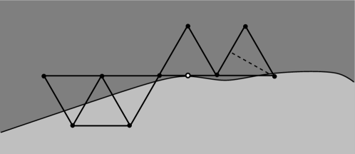
Figure 8. An edge of $\alpha$ either belongs to a triangle with no vertex in $\tilde{U}$, or to a triangle with a single vertex in $\tilde{U}$. In either case, the edge cannot be nearly perpendicular to $\tilde{\gamma}$.

Hence the edges of $\Sigma_{+}$ are inclined at an angle that is bounded away from being horizontal. So if $\pi(v)$ is the horizontal projection of $v\in\Sigma_{+}$ onto $\tilde{\Sigma}_{+}$, then $\pi$ defines a homeomorphism $\Sigma_{+}\to\tilde{\Sigma}_{+}$. We may extend $\pi$ to a homeomorphism $\pi\colon S\to\tilde{S}$ that linearly maps any horizontal segment of $S$ onto the horizontal segment of $\tilde{S}$ at the same imaginary part. In particular, $\pi$ agrees with the identity on $\Sigma_{-}$. It follows easily from the above that, for small $\varepsilon$, the map $\pi$ is $K_{2}$-quasiconformal, where $K_{2}$ is a universal constant. Moreover, the length of the elements of $\tilde{E}_{+}\mathrel{\vbox{\hbox{\scriptsize.}\hbox{\scriptsize.}}}=\pi(E_{+})$ tends to zero as $\varepsilon\to 0$, and adjacent intervals have comparable lengths, up to a universal multiplicative constant $\lambda>1$.

Let $\tilde{e}$ be an element of $\tilde{E}_{+}$. Then there is a unique homeomorphism $\psi_{1}\colon\tilde{e}\to\tilde{e}$ that fixes the endpoints of $\tilde{e}$ such that $\Phi^{\gamma}\circ\exp\circ\pi^{-1}\circ\psi_{1}$ is length-respecting on $\tilde{e}$. Note that this defines a homeomorphism $\psi_{1}\colon\tilde{\Sigma}_{+}\to\tilde{\Sigma}_{+}$. Applying Koebe’s theorem again, we see that the derivative of $\psi_{1}$ on $\tilde{e}$ tends to $1$ uniformly as $\varepsilon\to 0$. Extend $\psi_{1}$ to a map $\psi_{1}\colon\tilde{S}\to\tilde{S}$ that agrees with the identity on $\Sigma_{-}$ and is linear on each horizontal segment of $\tilde{S}$. By the above fact on the derivative of $\psi_{1}$ on $\tilde{\Sigma}_{+}$, the dilatation of the extension tends to $1$ as $\varepsilon\to 0$.

Finally, let $\psi_{2}\colon\tilde{S}\to\tilde{S}$ be the real-affine map that is the identity on $\tilde{\Sigma}_{-}$ and a translation on $\tilde{\Sigma}_{+}$ that maps the point of $\pi(V_{+})$ with smallest imaginary part to $\log R^{\gamma}/2$. If $K_{1}>K_{2}$, then the composition $\Psi\mathrel{\vbox{\hbox{\scriptsize.}\hbox{\scriptsize.}}}=\psi_{2}\circ\psi_{1}\circ\pi$ is $K_{1}$-quasiconformal for sufficiently small $\varepsilon$.

Since each of the maps $\psi_{2}$, $\psi_{1}$ and $\pi$ satisfies a and b, so does $\Psi$. Claim c holds by choice of $\psi_{2}$. We have $\Psi(E_{+})=\tilde{E}_{+}$, and the latter set satisfies d and e, as noted above. Finally, f holds by definition of $\psi_{1}$. This concludes the proof of the claim. ∎

Now consider the rectangle

$$Q\mathrel{\vbox{\hbox{\scriptsize.}\hbox{\scriptsize.}}}=Q^{\gamma}\mathrel{\vbox{\hbox{\scriptsize.}\hbox{\scriptsize.}}}=\{a+ib\colon 0\leq a\leq\log R^{\gamma}/2\text{ and }0\leq b\leq 2\pi\}.$$

The set $A_{+}\mathrel{\vbox{\hbox{\scriptsize.}\hbox{\scriptsize.}}}=\Psi(V_{+})\cap Q$ is a bounded-geometry partition of the left vertical side of $Q$. Set

$$A_{-}\mathrel{\vbox{\hbox{\scriptsize.}\hbox{\scriptsize.}}}=\{2\pi ij/d^{\gamma}\colon j=0,\dots,d^{\gamma}\};$$

this provides a partition of the right side of $Q$. By the claim, and since $d^{\gamma}\geq\Delta(R^{\gamma})$, all of the edges of the two partitions have length at most $2\pi\log R^{\gamma}$. It follows easily that we can extend $A_{+}\cup A_{-}$ to a bounded-geometry partition of $\partial Q$ in the sense of Proposition 3.4, where furthermore the partition of the upper and lower boundary agree up to translation by $2\pi i$. Now apply Proposition 3.4 to obtain a triangulation $\mathcal{Q}^{\gamma}$ of $Q=Q^{\gamma}$, where the angles of all triangles are bounded below by $\vartheta_{0}$. Observe that, in particular, no vertex is incident to more than $s_{1}\mathrel{\vbox{\hbox{\scriptsize.}\hbox{\scriptsize.}}}=\lfloor 2\pi/\vartheta_{0}\rfloor$ edges.

Map $\mathcal{Q}^{\gamma}$ to an equilateral surface $E^{\gamma}$ by a homeomorphism $g^{\gamma}$ that is real-affine on each triangle. Then $g^{\gamma}$ is $K_{3}$-quasiconformal, where $K_{3}$ depends only on $\vartheta_{0}$, and hence is a universal constant. We now form an equilateral surface as the union of $\tilde{E}$ and all $E^{\gamma}$, by identifying each boundary edge $e$ of $\tilde{E}$ on $\alpha(\gamma)$ with the corresponding edge $g^{\gamma}(\Psi(\operatorname{Log}((\Phi^{\gamma})^{-1}(e))))$ of $E^{\gamma}$. (Here $\operatorname{Log}$ is the branch of the logarithm taking imaginary parts between $0$ and $2\pi$.)

By the length-respecting property of $\Psi$, the function

$$g\colon\overline{U}\to E;z\mapsto\begin{cases}z&\text{if }z\in\tilde{E}\\ g^{\gamma}(\Psi(\operatorname{Log}((\Phi^{\gamma})^{-1}(z))))&\text{if }z\in E^{\gamma}\end{cases}$$

is continuous, and hence a $K_{0}\mathrel{\vbox{\hbox{\scriptsize.}\hbox{\scriptsize.}}}=K_{1}\cdot K_{3}$-quasiconformal homeomorphism which is conformal on $\tilde{E}$. Every vertex of $E$ is incident to at most $\max(6,d_{1}+4)$ edges. Finally, for any edge of $\Xi_{d^{\gamma}}$, we have

$$g\circ\varphi^{\gamma}=g^{\gamma}\circ\operatorname{Log}$$

on $E$. $\operatorname{Log}$ takes $e$ to one of the complementary intervals of $A_{-}$ in length-respecting fashion; this interval in turn is one of the edges of the triangulation $\mathcal{Q}^{\gamma}$. The restriction of $g^{\gamma}$ to this edge is a real-affine map, and hence length-respecting. This establishes b and completes the proof when $U$ has genus $0$.

If $U$ has positive genus $g>0$, then by definition $g$ is the largest number such that there are $g$ pairwise disjoint closed curves $\beta_{1},\dots,\beta_{g}\subset U$ such that

$$\tilde{U}\mathrel{\vbox{\hbox{\scriptsize.}\hbox{\scriptsize.}}}=U\setminus\bigcup_{i=1}^{g}\beta_{i}$$

is connected. We may choose the $\beta_{i}$ to be analytic. Let $\psi_{i}\colon S^{1}\to\beta_{i}$ be analytic parameterisations, which extend to analytic biholomorphic maps

$$\psi_{i}\colon\mathbb{A}(R_{i})\to A_{i}\subset U$$

for some $R_{i}>1$. We choose the $R_{i}$ sufficiently small to ensure that the closures of the annuli $A_{i}$ are pairwise disjoint, and also disjoint from the closures of the $A^{\gamma}$, and that additionally their combined $\rho$-area is at most $\eta$.

Clearly $\tilde{U}$ has genus $0$. We can think of $\tilde{U}$ as a hemmed Riemann surface, whose boundary curves are those inherited from $U$, together with two copies $\beta_{i}^{+}$ and $\beta_{i}^{-}$ of each $\beta_{i}$. The boundary parameterisations are given by

$$\varphi^{\beta_{i}^{-}}\colon\mathbb{A}^{-}(R_{i})\to\tilde{U};\quad z\mapsto\psi_{i}(z)\qquad\text{and}\qquad\varphi^{\beta_{i}^{+}}\colon\mathbb{A}^{-}(R_{i})\to\tilde{U};z\mapsto\psi_{i}(1/z).$$

Now apply Proposition 3.2 to the genus $0$ surface $\tilde{U}$, with constant $\eta/2$, where we take $d^{\beta_{i}^{+}}=d^{\beta_{i}^{-}}\geq\Delta(R_{i})$ for each $i$. We obtain an equilateral surface-with-boundary $\tilde{E}$ and a quasiconformal map $\tilde{g}\colon\tilde{U}\to\tilde{E}$. For each edge $e$ of the partition of $\beta_{i}$ given by $\psi_{i}(\Xi_{d^{\beta_{i}}})$, there are two corresponding intervals $e_{+}$ and $e_{-}$ on $\beta_{i}^{+}$ and $\beta_{i}^{-}$. Identifying the edges $g(e_{+})$ and $g(e_{-})$ on $\tilde{E}$, for every edge $e$, we obtain a new equilateral surface-with-boundary $E$. Condition b ensures that $\tilde{g}$ induces a homeomorphism $g\colon U\to E$ with the desired properties. ∎

4. Corrections on Riemann surfaces

As previously mentioned, our goal is to build the desired triangulations of the non-compact surface $X$ “piece by piece” on finite pieces (in the sense of Definition 2.1) of $X$, applying the construction of the preceding section. Recall that we may “straighten” these triangulations by a quasiconformal map to obtain an equilateral triangulation. This straightening changes the surface on which the triangulation is defined, but by Proposition 3.2 the dilatation of the quasiconformal maps in question is bounded and supported on sets of small area. Our goal is now to justify that the change to the complex structure is so small that the resulting perturbed piece can be re-embedded into our original surface $X$.

4.1 Proposition (Realising quasiconformal changes).

Let $X$ be a Riemann surface, equipped with a conformal metric $\rho$, and let $S\subsetneq X$ be an analytically bounded finite piece of $X$.

Let $0<K<1$, and let $\delta>0$. Then there is a constant $\eta>0$ with the following property. Let $\mu$ be a Beltrami form on $S$ whose support $\operatorname{supp}(\mu)$ has area at most $\eta$ (with respect to the metric on $X$) and whose dilatation is bounded by $K$. Then there is a quasiconformal homeomorphism

$$\psi\colon S\to\psi(S)\subset X$$

whose complex dilatation is $\mu$, which is isotopic to the identity and which satisfies

$$\operatorname{dist}(z,\psi(z))<\delta$$

for all $z\in S$.

4.2 Lemma.

To establish Proposition 4.1, it is sufficient to prove it in the special case where $X$ is compact and hyperbolic, and $\rho$ is the hyperbolic metric on $X$.

Proof.

If $X$ is not compact, let $\tilde{S}$ be a larger finite piece of $X$, extending $S$ by a small annulus at each boundary curve; so $\overline{S}\subset\tilde{S}\subset X$. Now form a new, compact, Riemann surface $\tilde{X}$ by glueing, into each boundary curve of $\tilde{S}$, a compact Riemann surface with a disc removed. By choosing at least one of these surfaces to have genus at least $2$, we ensure that $\tilde{X}$ is hyperbolic.

Let $\tilde{\rho}$ be the hyperbolic metric on $\tilde{X}$. Since $\rho$ and $\tilde{\rho}$ are comparable on the closure of $\tilde{S}$, there is $\tilde{\delta}>0$ with the following property. If $z\in S$ and $w\in\tilde{X}$ are such that $\operatorname{dist}_{\tilde{\rho}}(z,w)<\tilde{\delta}$, then $w\in\tilde{S}$ and $\operatorname{dist}_{\rho}(z,w)<\delta$.

Suppose that Proposition 4.1 has been proved for the compact surface $\tilde{X}$; we apply it with $S$, $K$ and $\tilde{\delta}$ to obtain a number $\tilde{\eta}>0$. Let $\eta>0$ be so small that any subset of $S$ of $\rho$-area at most $\eta$ has $\tilde{\rho}$-area at most $\tilde{\eta}$. (Again, this is possible by comparability of the Riemannian metrics.) Then $\eta$ satisfies the conclusion of Proposition 4.1 for $X$, $S$, $K$ and $\delta$. ∎

So it remains to establish Proposition 4.1 for $X$ compact and hyperbolic. To do so, we require some well-known results from the theory of Riemann surfaces, quasiconformal mappings and Teichmüller spaces. Let us begin with two simple facts related to the compactness of quasiconformal mappings.

4.3 Lemma (Compactness of quasiconformal mappings).

Let $X$ be a compact hyperbolic Riemann surface, let $K\geq 1$, and let $\psi_{n}\colon X\to X$ be a sequence of $K$-quasiconformal self-maps of $X$. Then there is a subsequence $(\psi_{n_{k}})_{k=0}^{\infty}$ that converges uniformly to a quasiconformal map $\psi\colon X\to X$. Moreover, if the dilatations $\mu_{n_{k}}$ of $\psi_{n_{k}}$ converge in measure to some Beltrami differential $\mu$, then $\mu$ is the dilatation of $\psi$.

Proof.

According to [Hub06, Theorem 4.4.1], the family of $K$-quasiconformal self-maps of $X$ is equicontinuous. Since $X$ is compact and the inverse of a $K$-quasiconformal map is $K$-quasiconformal, the family is indeed compact, proving the first claim.

The second claim follows from [Leh87, Theorem I.4.6] by lifting the maps to the disc via the universal covering map $\pi\colon\mathbb{D}\to X$. (Recall that, if $\mu_{n_{k}}\to\mu$ in measure, then there is a subsequence along which it converges almost everywhere.) ∎

4.4 Lemma (Area distortion).

Let $X$ be a compact hyperbolic Riemann surface, with its hyperbolic metric $\rho_{X}$, and let $K\geq 1$ and $\vartheta>0$. Then there is $\eta>0$ with the following property: If $E\subset X$ is compact with $\operatorname{area}_{X}(E)\leq\eta$, then $\operatorname{area}_{X}(\psi(E))\leq\vartheta$ for all $K$-quasiconformal maps $\psi\colon X\to X$.

Proof.

It was first observed by Bojarski [Boy55] that $K$-quasiconformal mappings, suitably normalised, distort area by a power depending only on $K$; see the first paragraph of [GR66]. Also compare [Ast94, EH95] for the optimal result. These results are normally stated for self-maps of the unit disc fixing the origin. In particular, the statement of Lemma 4.4 holds when $X$ is replaced by $\mathbb{D}$, equipped with the Euclidean metric $\rho_{\mathbb{C}}$, and $\psi\in\Psi_{\mathbb{D}}$, where $\Psi_{\mathbb{D}}$ consists of all $K$-quasiconformal self-maps of $\mathbb{D}$ fixing the origin.

Now let $X$ be compact and hyperbolic, and let $\pi\colon\mathbb{D}\to X$ be a universal covering. Let $A\subset\mathbb{D}$ with $0\in A$ be a fundamental hyperbolic polygon for the deck transformations of $\pi$. If $\psi\colon X\to X$ is $K$-quasiconformal, then we may lift $\psi$ to a quasiconformal map $\tilde{\psi}\colon\mathbb{D}\to\mathbb{D}$ with $\pi\circ\tilde{\psi}=\psi\circ\pi$, and such that $\tilde{\psi}(0)\in A$. Let $\alpha\colon\mathbb{D}\to\mathbb{D}$ be the Möbius transformation that maps $\tilde{\psi}(0)$ to $0$; then

$$\varphi\mathrel{\vbox{\hbox{\scriptsize.}\hbox{\scriptsize.}}}=\alpha\circ\tilde{\psi}\in\Psi_{\mathbb{D}}.$$

The set $\Psi_{\mathbb{D}}$ is compact by [Hub06, Corollary 4.4.3]; it follows that there is $r$, depending only on $A$ and $K$, such that $\varphi(A)\subset D(0,r)$. The Euclidean and hyperbolic metrics are comparable on $\overline{D(0,r)}$ by a factor of at most $C\mathrel{\vbox{\hbox{\scriptsize.}\hbox{\scriptsize.}}}=2/(1-r^{2})$.

Let $\vartheta>0$. By Bojarski’s observation, there is $\eta>0$ (depending on $K$ and $r$) such that

(4.1) $$\operatorname{area}_{\mathbb{C}}(\varphi(\tilde{E}))\leq\frac{\vartheta\cdot(1-r^{2})^{2}}{4}$$

whenever $\tilde{E}\subset\mathbb{D}$ has area at most $\vartheta$.

Now let $E\subset X$ have hyperbolic area at most $\eta$, and let $\tilde{E}=\pi^{-1}(E)\cap\overline{A}$. Then

$$\operatorname{area}_{\mathbb{C}}(\tilde{E})<\operatorname{area}_{\mathbb{D}}(\tilde{E})=\operatorname{area}_{X}(\tilde{E})\leq\eta\qquad\text{and hence}$$

$$\operatorname{area}_{X}(\psi(E))=\operatorname{area}_{\mathbb{D}}(\tilde{\psi}(\tilde{E}))=\operatorname{area}_{\mathbb{D}}(\varphi(\tilde{E}))\leq\frac{4}{(1-r^{2})}\cdot\operatorname{area}_{\mathbb{C}}(\varphi(\tilde{E}))\leq\vartheta$$

by (4.1). ∎

If $X$ is a hyperbolic Riemann surface, we denote by $\mathcal{T}(X)$ the Teichmüller space of $X$. Recall that $\mathcal{T}(X)$ can be defined as the set of equivalence classes $[\mu]_{T}$ of bounded measurable Beltrami differentials with $\lVert\mu\rVert_{\infty}<1$ [Hub06, Proposition 6.4.11]. Here two such differentials $\mu$ and $\nu$ are equivalent if there is a quasiconformal homeomorphism $\psi\colon X\to X$, isotopic to the identity relative the ideal boundary of $X$, such that $\psi^{*}(\nu)=\mu$ [Hub06, Proposition 6.4.11]. Here $\psi^{*}(\nu)$ is the pull-back of the differential $\nu$ by $\psi$; see [Hub06, Definition 4.8.10 and Formula 4.8.34].

Alternatively, lift $\mu$ and $\nu$ to $\mathbb{D}$ via the universal covering map. Then $\nu\in[\mu]_{T}$ if and only if the solutions $\varphi_{\mu},\varphi_{\nu}\colon\mathbb{D}\to\mathbb{D}$ of the corresponding Beltrami equations, normalised to fix $0$ and $1$, agree on $\partial\mathbb{D}$. $\mathcal{T}(X)$ is a complex Banach manifold, which is finite-dimensional if and only if $X$ is a compact surface with at most finitely many punctures removed; see [Hub06, Section 6.5].

4.5 Lemma.

Let $X$ be a compact Riemann surface, let $K\geq 1$, and let $(\mu_{n})_{n=0}^{\infty}$ be Beltrami differentials on $X$ of dilatation at most $K$.

Then $[\mu_{n}]_{T}\to[0]_{T}$ in Teichmüller space if and only if there are representatives $\nu_{n}\in[\mu_{n}]_{T}$ that converge to $0$ in measure.

Remark 1.

We shall only require the “if” direction. Note that this direction is false when $\mathcal{T}(X)$ is infinite-dimensional; compare [Gar84, Section 7].

Proof.

We use the Teichmüller metric on $\mathcal{T}(X)$; see [Hub06, Proposition and Definition 6.4.4]. With respect to this metric, the distance between $[\mu_{n}]_{T}$ and $[0]_{T}$ is $\log K$, where $K$ is the infimum of the dilatations of $\mu\in[\mu_{n}]$. In particular, if $[\mu_{n}]_{T}\to[0]_{T}$, then there are representatives of $[\mu_{n}]$ whose maximal dilatation converges to $1$. Hence these differentials converge to $0$ in measure.

For the “if” direction, note that the points having Teichmüller distance at most $\log K$ from $[0]_{T}$ is compact. (It is here that we use the fact that our Teichmüller space is finite-dimensional.) Now lift the Beltrami differentials $\mu_{n}$ to the universal cover and solve the Beltrami equation, obtaining $K$-quasiconformal maps $\varphi_{\mu_{n}}\colon\mathbb{D}\to\mathbb{D}$ fixing $0$ and $1$. By [Leh87, Theorem I.4.6], the only limit function of $\varphi_{\mu_{n}}$ as $n\to\infty$ is given by the identity, showing that indeed $[\mu_{n}]_{T}\to[0]_{T}$. ∎

We also require a result concerning the tangent space of $\mathcal{T}(X)$ at $X$, which is represented by infinitesimal classes $[\mu]_{B}$ of bounded measurable Beltrami differentials. By definition, $\mu\in[0]_{B}$ if

(4.2) $$\langle\mu,q\rangle\mathrel{\vbox{\hbox{\scriptsize.}\hbox{\scriptsize.}}}=\int_{X}\mu\cdot q=0$$

for all $q\in A^{1}(X)$, and $\mu\in[\nu]_{B}$ are infinitesimally equivalent if $\mu-\nu\in[0]_{B}$. Here $A^{1}(X)$ is the Bergman space of integrable holomorphic quadratic differentials on $X$. In fact, the pairing (4.2) induces an isomorphism between the tangent space to Teichmüller space and the dual space of $A^{1}(X)$ [Hub06, Proposition 6.6.2].

4.6 Lemma.

Let $X$ be a compact hyperbolic Riemann surface, $D\subset X$ a non-empty sub-surface, and let $\mu$ be a Beltrami differential on $X$. Then there is $\nu\in[\mu]_{B}$ such that $\nu=0$ a.e. on $X\setminus D$.

Proof.

Let $\varphi$ be the linear functional on $A^{1}(X)$ induced by $\mu$ via the pairing (4.2).

The restriction of any element of $A^{1}(X)$ to $D$ is an element of $A^{1}(D)$. So we can think of $A^{1}(X)$ as a finite-dimensional linear subspace of $A^{1}(D)$. Since the space is finite-dimensional, the linear functional $\varphi$ is continuous also with respect to the norm on $A^{1}(X)$ induced from that of $A^{1}(D)$. By the Hahn-Banach theorem, $\varphi$ extends to a continuous linear map $\tilde{\varphi}\colon A^{1}(D)\to\mathbb{C}$. By [Hub06, Proposition 6.6.2], this functional $\tilde{\varphi}$ is generated by some Beltrami differential $\tilde{\nu}$ on $D$.

Extend $\tilde{\nu}$ to $X$ by setting it to be $0$ outside of $D$. Then $\tilde{\nu}$ is in the same infinitesimal class as $\mu$ by construction, and we are done. ∎

Now we are ready to prove Proposition 4.1.

Proof of Proposition 4.1.

By Lemma 4.2, we may assume that $X$ is compact and hyperbolic, and endowed with the hyperbolic metric. Let $D$ be an open disc in $X\setminus\overline{S}$. Let $\hat{\mathcal{V}}$ denote the set of Beltrami differentials supported on $D$ and whose dilatation is bounded by $K$, and let $\mathcal{V}\subset\mathcal{T}(X)$ be the corresponding subset of Teichmüller space. The projection map $\pi\colon\mu\to[\mu]_{T}$ from Beltrami differentials to Teichmüller space is analytic [Hub06, Theorem 6.5.1]. The derivative at $[0]_{T}$ of this map is precisely the projection $\mu\to[\mu]_{B}$ [Hub06, Corollary 6.6.4]. Hence Lemma 4.6 implies that the restriction $\pi\colon\hat{\mathcal{V}}\to\mathcal{V}$ is a submersion near $[0]_{T}$, and therefore covers a neigbourhood of $[0]_{T}$ in $\mathcal{T}(X)$.

Indeed, recall that $\mathcal{T}(X)$ is finite-dimensional, so by Lemma 4.6 there are Beltrami differentials $\mu_{1}\dots,\mu_{n}\in\hat{\mathcal{V}}$ whose infinitesimal classes form a basis of the tangent space of $\mathcal{T}(X)$ at $[0]_{T}$. Consider the finite-dimensional subset $\mathcal{U}=\langle\mu_{1},\dots,\mu_{n}\rangle\cap\hat{\mathcal{V}}$; then the derivative at $[0]_{T}$ of $\pi\colon\mathcal{U}\to\mathcal{V}$ is invertible, and the claim follows by the inverse mapping theorem.

By Lemma 4.5, if $\eta$ is sufficiently small, then $[\mu]_{T}\in\mathcal{V}$ for any Beltrami differential $\mu$ on $X$ which has maximal dilatation at most $K$ and is supported on a set of measure less than $\eta$. So for any such $\mu$, there is a Beltrami differential $\nu\in\hat{\mathcal{V}}$ and an at most $K^{2}$-quasiconformal map $\psi\colon X\to X$, isotopic to the identity, such that $\psi^{*}(\nu)=\mu$.

Let $\mu_{n}$ be a sequence of Beltrami differentials on $S$ of dilatation bounded by $K$, and such that the area of the support of the dilatation tends to $0$ as $n\to\infty$. Furthermore, let $D_{k}\subset X\setminus\overline{S}$ be a shrinking sequence of discs whose area tends to zero.

For $n$ sufficiently large, we can construct a map $\psi_{n}$ as above, using $D=D_{k(n)}$, with $k(n)\to\infty$ as $n\to\infty$. Then the support of the dilatation $\tilde{\mu}_{n}$ of $\psi_{n}$ is contained in the union of the support of $\mu_{n}$ (whose area tends to zero) and the set $\psi_{n}^{-1}(D_{k(n)})$. By Lemma 4.4, the area of the latter set also tends to zero as $n\to\infty$.

By Lemma 4.3, every limit function of $(\psi_{n})$ as $n\to\infty$ is a conformal automorphism of $X$; since each $\psi_{n}$ is isotopic to the identiy, so are the limit functions. But a non-trivial conformal isomorphism $\varphi$ of $X$ cannot be isotopic to the identity (this result is usually attributed to Hurwitz). Indeed, if we lift $\varphi$ to the universal cover, we obtain a Möbius transformation $M$ on the disc; $\varphi$ is isotopic to the identity if and only if the boundary values of $M$, and therefore $M$ itself, agree with the identity; compare [Hub06, Proposition 6.4.9].

So $\psi_{n}$ converges to the identity. It follows that, by choosing $\eta$ sufficiently small in the statement of the proposition, the map $\psi$ we have constructed can be chosen as close to the identity as desired. In particular, we can ensure that $\psi^{-1}(D)\cap S=\emptyset$, and the restriction $\psi|_{S}$ solves the Beltrami equation for $\mu$, as desired. ∎

Remark.

Recent work of Kahn, Pilgrim and Thurston [KPT15] more generally describes when a topologically finite Riemann surface can be embedded into another, using an extremal length criterion. This can also be used to deduce Proposition 4.1, but the approach above is more elementary.

Finally, we record the following version of Lemma 4.4, for application on compact subsets of non-compact surfaces.

4.7 Proposition (Area distortion).

Let $X$ be a Riemann surface, equipped with a conformal metric $\rho$, and let $S\subsetneq X$ be a finite-type piece of $X$. Let $K\geq 1$ and let $B\subset S$ be compact. Then there is $\varepsilon>0$ and a function $\vartheta\colon(0,\infty)\to(0,\infty)$ with $\vartheta(t)\to 0$ as $t\to 0$, such that the following holds. Suppose that $\psi$ is a $K$-quasiconformal mapping from $S$ into $X$ such that $\operatorname{dist}_{\rho}(\psi(z),z)\leq\varepsilon$ for all $z\in S$. Then, for all $A\subset B$,

$$\operatorname{area}_{\rho}(\psi(A))\leq\vartheta_{\rho}(\operatorname{area}(A)).$$

Proof.

We can deduce the claim by applying Lemma 4.4 to a compact hyperbolic Riemann surface $\tilde{X}$ containing $S$, obtained exactly as in the proof of Lemma 4.2.

Let $\hat{S}\supset B$ be a slightly smaller finite-type piece $\hat{S}\subset S$. If $\varepsilon$ is chosen sufficiently small, we have $\psi(\hat{S})\subset S$ and we may extend $\psi|_{\hat{S}}$ to a $\tilde{K}$-quasiconformal map $\tilde{X}\to\tilde{X}$ which is the identity off $S$. Furthermore – again for sufficiently small $\varepsilon$ – the constant $\tilde{K}$ is independent of $\psi$. Now the claim follows from Lemma 4.4. ∎

5. Construction of equilateral triangulations

Our proof of Theorem 1.2 relies on a decomposition of our non-compact Riemann surface $X$ into analytically bounded finite pieces; see Figure 9

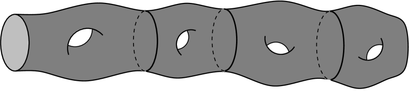
Figure 9. A decomposition as in Proposition 5.1, for an infinite-genus Riemann surface $X$.

5.1 Proposition.

Every non-compact Riemann surface $X$ can be written as

$$X=\bigcup_{j=0}^{\infty}\overline{U_{j}},$$

where the $U_{j}$ are pairwise disjoint analytically bounded finite pieces of $X$, such that every boundary curve $\gamma$ of $U_{j}$ is also a boundary curve of exactly one other piece $U_{j^{\prime}}$ ($j^{\prime}\neq j$).

Proposition 5.1 is a purely topological consequence of Radó’s theorem. Since we are not aware of a modern elementary account of this nature, we give the simple deduction below. The existence of a decomposition appears to have been first observed – for general open, triangulable, not necessarily orientable surfaces – by Kerékjártó in 1923 [vK23, §5.1, pp 166–167]. However, for his application (the topological classification of open surfaces), Kerékjártó requires additional properties of the decomposition, which means that some additional care is required in the construction.

Though favourably reviewed by Lefschetz in 1925 [Lef25], in subsequent years Kérekjártó’s work has been criticised, sometimes harshly [Fre73], for a lack of rigour. In particular, Richards [Ric63] observes that the justification for Kerékjártó’s classification theorem contains gaps (which Richards fills). Nonetheless, Kérekjárto’s argument for the existence of the decomposition is correct, if somewhat informal. Of course, much more precise statements are known, particularly in the case of Riemann surfaces; see e.g. [AR04].

Proof of Proposition 5.1.

It is equivalent to show that $X$ can be written as the increasing union of analytically bounded finite pieces $(X_{j})_{j=0}^{\infty}$ with $\overline{X_{j}}\subset X_{j+1}$. Indeed, the desired decomposition then consists of $X_{0}$ together with the connected components of $X_{j+1}\setminus\overline{X_{j}}$, which are themselves finite pieces of $X$.

Let $\mathcal{T}$ be a triangulation of $X$, which exists by Radó’s theorem. Fix a triangle $K_{0}\in\mathcal{T}$; recall that $K_{0}\subset X$ is compact. We inductively define a sequence $(K_{j})_{j=0}^{\infty}$ of compact, connected sets by

$$K_{j+1}\mathrel{\vbox{\hbox{\scriptsize.}\hbox{\scriptsize.}}}=\bigcup\{T\in\mathcal{T}\colon T\cap K_{j}\neq\emptyset\}.$$

Then $\bigcup K_{j}=X$, and each interior $\operatorname{int}(K_{j})$ is connected, contains $K_{j-1}$, and is a finite piece of $X$. Hence we may shrink $K_{j}$ (whose boundary may not be analytic) slightly to obtain an analytically bounded finite piece $X_{j}$ that still contains $K_{j-1}$. ∎

Proof of Theorem 1.2.

Let $X$ be a non-compact Riemann-surface; we shall construct an equilateral triangulation on $X$. Let $\rho$ be a complete conformal metric on $X$; for example, a metric of constant curvature. As mentioned in the introduction, Theorem 1.2 is trivial when $X$ is Euclidean (and hence either the plane or the punctured plane). So we could assume that $X$ is hyperbolic, and $\rho$ the hyperbolic metric. However, our construction works equally well regardless of the nature of the metric, so we shall not require this assumption.

For the remainder of the section, fix a decomposition $(U_{j})_{j=0}^{\infty}$ of $X$ into analytically bounded finite pieces, as in Proposition 5.1.

Let $\Gamma$ be the set of all boundary curves of the $U_{j}$. For every $\gamma\in\Gamma$, there are unique $j_{1}<j_{2}$ such that $\gamma$ is on the boundary of $U_{j_{1}}$ and of $U_{j_{2}}$. We say that $\gamma$ is an outer curve of $U_{j_{1}}$ and an inner curve of $U_{j_{2}}$, and write $\iota_{-}(\gamma)\mathrel{\vbox{\hbox{\scriptsize.}\hbox{\scriptsize.}}}=j_{1}$ and $\iota_{+}(\gamma)\mathrel{\vbox{\hbox{\scriptsize.}\hbox{\scriptsize.}}}=j_{2}$. For $j\geq 0$, let $\Gamma^{-}(U_{j})$ denote the set of inner boundary curves of $U_{j}$, and let $\Gamma^{+}(U_{j})$ denote the set of all outer boundary curves of $U_{j}$.

We may assume that the pieces $U_{j}$ are numbered such that

$$X_{j}=\bigcup_{k=0}^{j}U_{k}\cup\bigcup\{\gamma\in\Gamma\colon\iota_{+}(\gamma)\leq j\}$$

is connected for all $j\geq 0$; hence $X_{j}$ is a finite piece of $X$. Let $\Gamma(X_{j})$ denote the boundary curves of $X_{j}$; that is,

$$\Gamma(X_{j})=\{\gamma\in\Gamma\colon\iota_{-}(\gamma)\leq j<\iota_{+}(\gamma)\}.$$

See Figure 10.

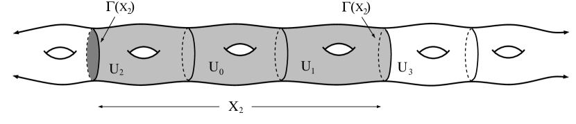
Figure 10. The definition of $X_{j}$ and its set of boundary curves $\Gamma(X_{j})$.

For each $\gamma$, we fix an analytic parameterisation $\varphi^{\gamma}\colon S^{1}\to\gamma$. Let $\hat{R}^{\gamma}>1$ be so small that $\varphi^{\gamma}$ extends to a conformal isomorphism from $\mathbb{A}(\hat{R}^{\gamma})$ onto an annulus $\hat{A}^{\gamma}$; we may assume that different $\hat{A}^{\gamma}$ have pairwise disjoint closures. Set

$$\hat{A}_{+}^{\gamma}\mathrel{\vbox{\hbox{\scriptsize.}\hbox{\scriptsize.}}}=\varphi^{\gamma}(\mathbb{A}_{+}(\hat{R}^{\gamma}))\qquad\text{and}\qquad\hat{A}_{-}^{\gamma}\mathrel{\vbox{\hbox{\scriptsize.}\hbox{\scriptsize.}}}=\varphi^{\gamma}(\mathbb{A}_{-}(\hat{R}^{\gamma})).$$

Precomposing by $z\mapsto 1/z$ and decreasing $\hat{R}_{\gamma}$ if necessary, we can ensure that $A_{+}^{\gamma}\subset U_{\iota_{+}(\gamma)}$ and $A_{-}^{\gamma}\subset U_{\iota_{-}(\gamma)}$. For $R\leq\hat{R}_{\gamma}$, we also define

$$A^{\gamma}(R)\mathrel{\vbox{\hbox{\scriptsize.}\hbox{\scriptsize.}}}=\varphi_{\gamma}(\mathbb{A}(R))\qquad\text{and}\qquad A^{\gamma}_{\pm}(R)\mathrel{\vbox{\hbox{\scriptsize.}\hbox{\scriptsize.}}}=\varphi_{\gamma}(\mathbb{A}_{\pm}(R)).$$

For example, $\hat{A}^{\gamma}=A^{\gamma}(\hat{R}_{\gamma})$.

We use these annuli to define annular extensions of $\overline{X_{j}}$ in $X$ as follows. Let $\hat{X}_{j}$ be the union of $\overline{X_{j}}$ and the annuli $\hat{A}^{\gamma}$ for all boundary curves $\gamma$ of $X_{j}$; i.e.,

$$\hat{X}_{j}=X_{j}\cup\bigcup\bigl{\{}(\gamma\cup\hat{A}^{\gamma}_{+})\colon\iota_{-}(\gamma)\leq j<\iota_{+}(\gamma)\bigr{\}}.$$

Then $X_{j}$ an analytically bounded finite piece of $\hat{X}_{j}$.

Fix the constant $K_{0}$ from Proposition 3.2. We define the desired triangulation piecewise, through an inductive construction. The underlying strategy can be described as follows.

Apply Proposition 3.2 to construct a $K_{0}$-quasiconformal function $g_{0}\colon U_{0}\to E_{0}$, where $U_{0}$ is considered as a hemmed surface with boundary parameterisations $\varphi^{\gamma}$, and $E_{0}$ is an equilateral surface-with-boundary. In the following, we shall use without comment the properties described in the conclusion of Proposition 3.2. In particular, the equilateral triangulation of $E_{0}$ has local degree bounded by $d_{0}$, and $g_{0}\circ\varphi^{\gamma}$ maps every edge of the partition $\Xi_{d^{\gamma}}$ to an edge of $E_{0}$ in length-respecting fashion. If the degrees $d^{\gamma}$ are sufficiently large, then the dilatation of $g_{0}$ is supported on a set of small area, and by Proposition 4.1, there is a quasiconformal map $\psi_{0}$ from $\hat{X}_{0}$ into $X$ such that $f_{0}\mathrel{\vbox{\hbox{\scriptsize.}\hbox{\scriptsize.}}}=g_{0}\circ\psi_{0}^{-1}$ is conformal, and $\psi_{0}$ is close to the identity.

Thus we have obtained an equilateral triangulation of the finite piece $\tilde{X}_{0}\mathrel{\vbox{\hbox{\scriptsize.}\hbox{\scriptsize.}}}=\psi_{0}(X_{0})$ of $X$, which is bounded by the curves $\psi_{0}(\gamma)$ for $\gamma\in\Gamma(X_{0})$. Consider the piece $\tilde{U}_{1}$ whose outer boundary curves are the outer boundary curves of $U_{1}$, and whose inner boundary curves are given by $\psi_{0}(\gamma)$ for $\gamma\in\Gamma^{-}(U_{1})$. Then $\tilde{U}_{1}$ is a hemmed Riemann surface, where for the inner curves we use the boundary correspondence given by

$$\varphi_{1}^{\gamma}(\zeta)\mathrel{\vbox{\hbox{\scriptsize.}\hbox{\scriptsize.}}}=\psi_{0}\left(\varphi^{\gamma}\left(\frac{1}{\zeta}\right)\right),$$

defined on some annulus $\mathbb{A}^{-}(R^{\gamma})$. Observe that

$$f_{0}\circ\varphi_{1}^{\gamma}$$

is length-respecting on $S^{1}$, for each $\gamma$.

We may apply Proposition 3.2 to this hemmed surface, using the same values $d^{\gamma}$ on the inner boundary curves of $\tilde{U}_{1}$ – assuming they were chosen sufficiently large in step $0$. We obtain a map $g\colon\tilde{U}_{1}\to E_{1}$. By the length-preserving properties of $g$ and $f_{0}$, it follows that $g$ extends $f_{0}$ continuously to a quasiconformal map $g_{1}$ from

$$Y_{1}\mathrel{\vbox{\hbox{\scriptsize.}\hbox{\scriptsize.}}}=\tilde{X}_{0}\cup\tilde{U}_{1}\cup\bigcup_{\gamma\in\Gamma^{-}(U_{1})}\psi_{0}(\gamma)\subset\hat{X}_{1}$$

to an equilateral surface $\mathcal{E}_{1}$, which is the union of $E_{0}$ and $E_{1}$, glued along corresponding boundary curves. Again, assuming that all degrees are sufficiently large, we straighten $g_{1}$ using a quasiconformal map $\psi_{1}$ from $\hat{X}_{1}$ into $X$. The result is an equilateral triangulation of the finite piece $\tilde{X}_{1}\mathrel{\vbox{\hbox{\scriptsize.}\hbox{\scriptsize.}}}=\psi_{1}(Y_{1})$, and we continue inductively.

More formally, the construction depends on a collection of numbers $(R^{\gamma})_{\gamma\in\Gamma}$, with $1<R^{\gamma}<\hat{R}^{\gamma}$, and positive integers $(d^{\gamma})_{\gamma\in\Gamma}$ with $d^{\gamma}\geq\Delta(R^{\gamma})$. (Here $\Delta$ is the function from Proposition 3.2.) After the $(j-1)$-th stage of the construction, we will have constructed the following objects.

1. $\tilde{X}_{j-1}$ is a finite piece of $X$, homotopic to $X_{j-1}$ and contained in $\hat{X}_{j-1}$.

2. For each boundary curve $\gamma\in\Gamma(X_{j-1})$, the corresponding boundary curve of $\tilde{X}_{j-1}$ is the image of $\gamma$ under a $K_{0}$-quasiconformal map $\Psi^{\gamma}_{j-1}$. This map is defined on $A^{\gamma}(R^{\gamma})$ and conformal on $A^{\gamma}_{+}(R^{\gamma})$; furthermore,

   $$\Psi^{\gamma}_{j-1}(A_{-}^{\gamma}(R^{\gamma}))\subset\tilde{X}_{j-1}\qquad\text{and}\qquad\Psi^{\gamma}_{j-1}(A_{+}^{\gamma}(R^{\gamma}))\cap\tilde{X}_{j-1}=\emptyset.$$

3. $\Psi^{\gamma}_{j-1}(A^{\gamma}(R^{\gamma}))\subset\hat{A}^{\gamma}$ for each $\gamma$ as in 2.

4. $f_{j-1}\colon\operatorname{cl}(\tilde{X}_{j-1})\to\mathcal{E}_{j-1}$ is a homeomorphism that is conformal on $\tilde{X}_{j-1}$, where $\mathcal{E}_{j-1}$ is a finite equilateral surface-with-boundary. For $\gamma\in\Gamma(X_{j-1})$, the map

   $$f_{j-1}\circ\Psi^{\gamma}_{j-1}\circ\varphi^{\gamma}$$

   maps each edge of the partition $\Xi_{d^{\gamma}}$ to a boundary edge of $\mathcal{E}_{j-1}$ in length-preserving fashion.

5. In $\mathcal{E}_{j-1}$, every inner vertex is incident to at most $2d_{0}-2$ edges, and every boundary vertex is incident to at most $d_{0}$ edges.

For $j=0$, we use the convention that $\tilde{X}_{-1}=\Gamma(X_{-1})=\mathcal{E}_{-1}=\emptyset$, so that the hypotheses are trivial.

The inductive construction proceeds as follows.

Step 1. We define $\tilde{U}_{j}$ to be the finite piece of $X$ bounded by the curves in $\Gamma^{+}(U_{j})$ and the curves $\Psi^{\gamma}_{j-1}(\gamma)$ for $\gamma\in\Gamma^{-}(U_{j})$. This piece becomes a hemmed surface when equipped with the boundary parameterisations $\varphi^{\gamma}$ for the boundary curves $\gamma\in\Gamma^{+}(U_{j})$ and

$$\varphi^{\gamma}_{j-1}(\zeta)\mathrel{\vbox{\hbox{\scriptsize.}\hbox{\scriptsize.}}}=\Psi^{\gamma}_{j-1}\left(\varphi^{\gamma}(1/\zeta)\right)$$

for the others.

Step 2. We apply Proposition 3.2 to obtain a quasiconformal map

$$g_{j}\colon\operatorname{cl}(\tilde{U}_{j})\to E_{j},$$

where $E_{j}$ is a finite equilateral surface-with-boundary, and every vertex of $E_{j}$ has local degree at most $d_{0}$. For each $\gamma\in\Gamma^{-}(U_{j})$, the function $g_{j}\circ\Psi^{\gamma}_{j-1}\circ\varphi^{\gamma}$ maps each edge of $\Xi_{d^{\gamma}}$ to an edge of $E_{j}$ in length-respecting fashion. (Note that the map $\zeta\mapsto 1/\zeta$ is itself length-respecting on $S^{1}$.)

Step 3. Next, we apply Proposition 4.1, where $S=\hat{X}_{j}$ and $\mu$ is the Beltrami differential of $g_{j}$ on $\tilde{U}_{j}$, and $0$ elsewhere. We obtain a quasiconformal homeomorphism $\psi_{j}\colon S\to\psi(S)\subset X$, isotopic to the identity. Of course, we can only apply Proposition 4.1 if the support of $\mu$ is sufficiently small; we show below that it is possible to ensure this by choosing the sequence $(R^{\gamma})_{\gamma\in\Gamma}$ appropriately.

Step 4. Finally, we define $\tilde{X}_{j}$, functions $\Psi^{\gamma}_{j}$, an equilateral surface $\mathcal{E}_{j}$ and a function $f_{j}\colon\operatorname{cl}(\tilde{X}_{j})\to\mathcal{E}_{j}$ such that 1, 2 and 4 hold (with $j-1$ replaced by $j$).

Firstly, set

$$Y_{j}\mathrel{\vbox{\hbox{\scriptsize.}\hbox{\scriptsize.}}}=\tilde{X}_{j-1}\cup\tilde{U}_{j}\cup\bigcup_{\gamma\in\Gamma^{-}(U_{j})}\Psi^{\gamma}_{j-1}(\gamma)\qquad\text{and}\qquad\tilde{X}_{j}\mathrel{\vbox{\hbox{\scriptsize.}\hbox{\scriptsize.}}}=\psi_{j}(Y_{j}).$$

Then $\tilde{X}_{j}$ is a finite piece of $X$, homotopic to $X_{j}$.

Note that

$$\Gamma(X_{j})=(\Gamma(X_{j-1})\setminus\Gamma^{-}(U_{j}))\cup\Gamma^{+}(U_{j}).$$

The boundary curves of $\tilde{X}_{j}$ are given by the curves $\Psi^{\gamma}_{j}(\gamma)$, where

(5.1) $$\Psi^{\gamma}_{j}=\psi_{j}\circ\Psi^{\gamma}_{j-1}$$

when $\gamma\in\Gamma(X_{j-1})\setminus\Gamma^{-}(U_{j})$ and $\Psi^{\gamma}_{j}=\psi_{j}$ when $\gamma\in\Gamma^{+}(U_{j})$. In (5.1), recall that $\psi_{j}$ is conformal outside of $\tilde{U}_{j}$, and hence on $\hat{A}_{\gamma}$ for $\gamma\in\Gamma(X_{j-1})\setminus\Gamma^{-}(U_{j})$. So $\Psi^{\gamma}$ is indeed $K_{0}$-quasiconformal on $A^{\gamma}(R^{\gamma})$ and conformal on $A^{\gamma}_{+}(R^{\gamma})$. It follows that 2 holds for our maps $\Psi^{\gamma}_{j}$.

Finally, let $\gamma\in\Gamma^{-}(U_{j})$, let $e$ be an edge of $\Xi_{d^{\gamma}}$, and consider $\tilde{e}\mathrel{\vbox{\hbox{\scriptsize.}\hbox{\scriptsize.}}}=\Psi_{j-1}^{\gamma}(\varphi^{\gamma}(e))$. Then $f_{j-1}(\tilde{e})$ is a boundary edge of $\mathcal{E}_{j-1}$, and $g_{j}(\tilde{e})$ is a boundary edge of $E_{j}$. We form an equilateral surface-with-boundary $\mathcal{E}_{j}$ by identifying these two boundary edges for each $\gamma$ and each $e$. We identify $\mathcal{E}_{j-1}$ and $E_{j}$ with their corresponding subsets of $\mathcal{E}_{j}$. Every boundary vertex of $\mathcal{E}_{j}$ is a boundary vertex of $\mathcal{E}_{j-1}$ or of $E_{j}$, and therefore has local degree at most $d_{0}$. Every inner vertex of $\mathcal{E}_{j}$ is either an inner vertex of $\mathcal{E}_{j_{1}}$ or of $E_{j}$, or it is a common boundary vertex of both. In the latter case, the vertex is connected to at most $d_{0}-2$ inner edges of $\mathcal{E}_{j-1}$, at most $d_{0}-2$ inner edges of $E_{j}$, and two common boundary edges of the two. This establishes 5 for $\mathcal{E}_{j}$.

Both $f_{j-1}$ and $g_{j}$ take values in $\mathcal{E}_{j}$. Let $\gamma$, $e$ and $\tilde{e}$ be as above, and define $\hat{e}=f_{j-1}(\tilde{e})=g_{j}(\tilde{e})$. By 4 and the observation on $g_{j}$ in Step 2, the map $g_{j}\circ f_{j-1}^{-1}$ is an isometry of the edge $\hat{e}$. Keeping in mind that $f_{j-1}$ and $g_{j}$ are orientation-preserving, and take values on opposite sides of $\hat{e}$ in $\mathcal{E}_{j}$, it follows that $g_{j}\circ f_{j-1}^{-1}=\operatorname{id}$ on $\hat{e}$. Thus

$$g\colon\operatorname{cl}(Y_{j})\to\mathcal{E}_{j};\quad z\mapsto\begin{cases}f_{j-1}(z)&\text{if }z\in\operatorname{cl}(\tilde{X}_{j-1})\\ g_{j}(z)&\text{if }z\in\operatorname{cl}(\tilde{U}_{j})\end{cases}$$

is a well-defined homeomorphism. $f_{j-1}$ is $K_{0}$-quasiconformal on $\tilde{X}_{j-1}$, and $g_{j}$ is $K_{0}$-quasiconformal on $\tilde{U}_{j}$. Since the common boundary curves $(\Psi_{j-1}^{\gamma}(\gamma))_{\gamma\in\Gamma^{-}(U_{j})}$ are quasicircles, $g$ is $K_{0}$-quasiconformal on all of $Y_{j}$.

Now define

$$f_{j}\mathrel{\vbox{\hbox{\scriptsize.}\hbox{\scriptsize.}}}=g\circ\psi_{j}^{-1}\colon\operatorname{cl}(\tilde{X}_{j})\to\mathcal{E}_{j}.$$

Then $f_{j}$ is conformal on $\tilde{X}_{j}$ and satisfies 4.

It remains to see that Proposition 4.1 can always be applied in Step 3, and that $\psi_{j}$ is sufficiently close to the identity that 3, and therefore 1, hold. This requires that the dilatation of the map $g_{j}$ can be chosen to be supported on a sufficiently small set. By Proposition 3.2, this dilatation is supported on the annuli $\Psi^{\gamma}_{j-1}(A_{+}^{\gamma}(R^{\gamma}))$ for inner curves of $U_{j}$ and on the annuli $\varphi^{\gamma}(A_{-}^{\gamma}(R^{\gamma})$ for outer curves of $U_{j}$, together with a set of negligible area. The area of the latter annuli can be made small simply by choosing $R^{\gamma}$ small enough.

For the former annuli, on the other hand, we must be slightly more careful. Indeed, the map $\Psi^{\gamma}$ is the composition of $\psi_{j-1}$, $\psi_{j-2}$, …, $\psi_{\iota^{-}(\gamma)}$. The last of these depends on $d^{\gamma}$, which in turn depends on $R^{\gamma}$. So $R^{\gamma}$ must be chosen so that the image $A_{-}^{\gamma}(R^{\gamma})$ under $\Psi^{\gamma}$ is small, independently of the choices that determine $\Psi^{\gamma}$. Happily, since the dilatation of $\Psi^{\gamma}$ is uniformly bounded, we can do so using the area distortion of quasiconformal mappings (Proposition 4.7).

To make all of this precise, for each $\gamma\in\Gamma$ choose annuli $\hat{A}^{\gamma}_{1}$ and $\hat{A}^{\gamma}_{2}$ with

$$\gamma\subset\hat{A}^{\gamma}_{1}\Subset\hat{A}^{\gamma}_{2}\Subset\hat{A}^{\gamma}.$$

We set

$$\varepsilon^{\gamma}_{1}\mathrel{\vbox{\hbox{\scriptsize.}\hbox{\scriptsize.}}}=\operatorname{dist}(\hat{A}^{\gamma}_{2},\partial\hat{A}^{\gamma}).$$

Also let $\varepsilon^{\gamma}_{2}$ be the constant $\varepsilon$ from Proposition 4.7, with $K=K_{0}$, $S=\hat{A}^{\gamma}_{2}$, and $B=\operatorname{cl}(\hat{A}^{\gamma}_{1})$. Also let $\vartheta=\vartheta^{\gamma}\colon(0,\infty)\to(0,\infty)$ be the function from the same proposition. So a $K_{0}$-quasiconformal map from $\hat{A}^{\gamma}_{2}$ into $X$ maps sets of area at most $\eta$ to sets of area at most $\vartheta^{\gamma}(\eta)$, provided that it does not move points by more than $\varepsilon^{\gamma}_{2}$. Define

$$\varepsilon^{\gamma}\mathrel{\vbox{\hbox{\scriptsize.}\hbox{\scriptsize.}}}=\min(1,\varepsilon^{\gamma}_{1},\varepsilon^{\gamma}_{2}).$$

Next, for $j\geq 0$, choose $\eta_{j}$ according to Proposition 4.1, where we use $S=\hat{X}_{j}$, $K=K_{0}$, and

$$\delta=\delta_{j}\mathrel{\vbox{\hbox{\scriptsize.}\hbox{\scriptsize.}}}=2^{-(j+1)}\cdot\min_{\gamma\in\Gamma(X_{j})}\varepsilon^{\gamma}.$$

Finally, choose $R^{\gamma}$ sufficiently close to $1$ to ensure that

• $A^{\gamma}(R^{\gamma})\subset\hat{A}^{\gamma}_{1}$,

• $\displaystyle{\operatorname{area}(A^{\gamma}_{-}(R^{\gamma}))\leq\frac{\eta_{\iota^{-}(\gamma)}}{2\#\Gamma(U_{\iota^{-}(\gamma)})}}$, and

• $\displaystyle{\vartheta^{\gamma}(\operatorname{area}(A^{\gamma}_{+}(R^{\gamma})))\leq\frac{\eta_{\iota^{+}(\gamma)}}{2\#\Gamma(U_{\iota^{+}(\gamma)})}}$.

Observe that this choice of $(R^{\gamma})_{\gamma\in\Gamma}$ depends only on the surface $X$, its metric $\rho$ and the decomposition $(U_{j})_{j\geq 0}$ of $X$ into finite pieces. We claim that, in our inductive construction, we can ensure

1. $\Psi_{j-1}^{\gamma}$ is defined on $\hat{A}^{\gamma}_{2}$, where it satisfies

   $$\operatorname{dist}(\Psi_{j-1}^{\gamma}(z),z)\leq(1-2^{-j})\cdot\varepsilon^{\gamma},$$

in addition to 1–4.

Observe that, by choice of $\varepsilon^{\gamma}_{1}$ and $R^{\gamma}$, 6 implies

(5.2) $$\Psi_{j-1}^{\gamma}(A^{\gamma}(R^{\gamma}))\subset\Psi_{j-1}^{\gamma}(\hat{A}^{\gamma}_{1})\subset\Psi_{j-1}^{\gamma}(\hat{A}^{\gamma}_{2})\subset\hat{A}^{\gamma}.$$

In particular, 3 and 1 follow.

In order to obtain 6, we use $\eta=\eta_{j}/2$ when applying Proposition 3.2 in Step 2 of the inductive construction. The dilatation of $g_{j}$ is then supported on the union of

1. a set of area at most $\eta$;

2. the annuli $A^{\gamma}_{-}(R^{\gamma})$ for the outer curves of $U_{j}$; i.e., those $\gamma\in\Gamma$ for which $\iota^{-}(\gamma)=j$;

3. the annuli $\Psi_{j-1}^{\gamma}(A^{\gamma}_{+}(R^{\gamma})$ for the inner curves of $U_{j}$, i.e. those $\gamma\in\Gamma$ for which $\iota^{+}(\gamma)=j$.

By choice of $R^{\gamma}$ and $\vartheta^{\gamma}$, and by (5.2), we see that each of the annuli in b and c has area at most

$$\frac{\eta_{j}}{2\#\Gamma(U_{j})}.$$

So the support of the dilatation has area at most $\eta_{j}$.

By choice of $\eta_{j}$, this implies that Proposition 4.1 can indeed by applied in Step 2, and $\psi_{j}$ moves points at most a distance of $\delta_{j}$. Now, using 6 for $\Psi_{j-1}$, it follows from the definition of $\Psi_{j}^{\gamma}$ that 6 also holds for $\Psi_{j}$. The inductive construction is complete.

To complete the proof, we claim that the functions $f_{j}$ converge to a conformal isomorphism $f$ between $X$ and an equilateral surface $\mathcal{E}$. To show this, fix $j\geq 0$ and define

$$\alpha_{n}\mathrel{\vbox{\hbox{\scriptsize.}\hbox{\scriptsize.}}}=\psi_{n}\circ\psi_{n-1}\circ\dots\circ\psi_{j}$$

for $n\geq j$. Then $\alpha_{n}$ is a quasiconformal map on $\hat{X}_{j}$, and

$$\operatorname{dist}(\alpha_{n}(z),\alpha_{n+1}(z))=\operatorname{dist}(\alpha_{n}(z),\psi_{n+1}\alpha_{n}((z)))\leq\delta_{n+1}\leq 1/2^{n+2}.$$

So the maps $\alpha_{n}$ form a Cauchy sequence, and converge to a non-constant quasiconformal map $\alpha$ on $\hat{X}_{j}$, and their inverses converge to $\alpha^{-1}$. By definition of $f_{n}$, we have

$$f_{n}\circ\alpha_{n}|_{\tilde{U}_{j}}=f_{n-1}\circ\alpha_{n-1}|_{\tilde{U}_{j}}=\dots=g_{j},$$

and hence $f_{n}\to g_{j}\circ\alpha^{-1}$ uniformly on the closure of $\tilde{U}_{j}$.

So $f_{n}$ converges to a conformal function

$$f\colon X\to\mathcal{E}\mathrel{\vbox{\hbox{\scriptsize.}\hbox{\scriptsize.}}}=\bigcup_{j=0}^{\infty}\mathcal{E}_{j}.$$

Hence $X$ is conformally equivalent to the (infinite) equilateral surface $\mathcal{E}$, and the proof of Theorem 1.2 is complete. ∎

Proof of Theorems 1.4 and 1.6.

By Theorem 1.2, there is an equilateral triangulation $\mathcal{T}$ on $X$. By Proposition 2.7, there is a Belyi function $f$ on $X$. This proves Theorem 1.4.

Moreover, the triangulation $\mathcal{T}$ has the property that no vertex is incident to more than $2d_{0}-2$ edges (recall 5 in the proof of Theorem 1.2). The Belyi function constructed in the proof of Proposition 2.7 has the property that every preimage of $-1$ has degree $2$, every preimage of $\infty$ has degree $3$. Furthermore, the preimages of $1$ are precisely the vertices of $\mathcal{T}$, and the components of $f^{-1}([-1,1))$ are the edges of $\mathcal{T}$. So every critical point of $f$ has degree at most $2d_{0}-2$. ∎

(a) Subdivision of a boundary triangle

(b) Subdividing all boundary triangles

Figure 11. Proof of Lemma 5.2.

It is intuitively clear that our proof of Theorem 1.2 involves infinitely many independent choices, leading to uncountably many different combinatorially different triangulations. To make this precise, and hence to prove Corollary 1.7, we will use the following strengthening of Proposition 3.2.

5.2 Lemma.

In Proposition 3.2, we may replace a by

1. There are universal constants $D_{0}\geq D_{1}>4$ with the following property. Every boundary vertex of $E$ has degree at least $D_{1}$ and at most $D_{0}$, and every inner vertex of $E$ has degree less than $D_{1}$.

Proof.

Let $\Delta$ be an equilateral triangle with vertices $A$, $B$, $C$. We may triangulate $T$ by adding $d_{0}$ vertices $v_{1},\dots,v_{d_{0}}$ inside $T$, where each $d_{i}$ is connected to $A$ and $B$ and also to $d_{i-1}$, with the convention that $v_{0}=C$. (See Figure 11(a).) Mapping these triangles in an affine manner to equilateral triangles, we obtain a quasiconformal map $h\colon T\to E_{0}$, where $E_{0}$ is an equilateral surface-with-boundary. On this surface, the two boundary vertices corresponding to $A$ and $B$ have degree $d_{0}+2$, while $C$ has degree $3$ and the interior vertices all have degree $3$ or $4$.

Let $\tilde{E}$ be the equilateral surface obtained in Proposition 3.2, and let $T$ be a boundary triangle; i.e., a triangle in $\tilde{E}$ that has an edge on $\partial\tilde{E}$. We may identify $T$ with $\Delta$ such that the boundary edge corresponds to the edge $AB$. We assume that $C$ is an interior vertex of $\tilde{E}$. (This is always true if we follow the construction in the proof of Proposition 3.2, but the argument is easily adapted if this is not the case.)

We can glue a copy of $E_{0}$ into $\tilde{E}$ in place of $T$, for every such triangle $T$. The result is a new equilateral surface $E$, and a quasiconformal homeomorphism $h_{1}\colon\tilde{E}\to E$, whose maximal dilatation coincides with that of $h$. Every boundary vertex of $\tilde{E}$ belongs to exactly two boundary triangles. Hence, on $E$, each of these vertices has local degree at least $D_{1}\mathrel{\vbox{\hbox{\scriptsize.}\hbox{\scriptsize.}}}=2+2d_{0}\geq 14$, and at most $D_{0}\mathrel{\vbox{\hbox{\scriptsize.}\hbox{\scriptsize.}}}=3d_{0}$. On the other hand, any interior vertex of $\tilde{E}$ belongs to at most $d_{0}$ triangles. Thus it arises as the vertex $C$ in the above construction for at most $d_{0}$ different triangles, and has degree at most $2d_{0}<D_{1}$ in $E$. Any new vertices in $E$ have degree at most $4<D_{1}$. This completes the proof. ∎

Proof of Corollary 1.7.

First suppose that $X$ is non-compact. Let $\mathcal{T}$ be an equilateral triangulation on $X$, and let $f\colon X\to\hat{\mathbb{C}}$ be the corresponding Belyi function from Proposition 2.7. The vertices and edges of $\mathcal{T}$ are given by $f^{-1}(-1)$ and $f^{-1}([-1,1))$, respectively. Hence it is enough to show that the proof of Theorem 1.2 can produce uncountably many different triangulations of $X$, no two of which agree up to a conformal isomorphism of $X$.

We use the notation from the proof of Theorem 1.2, but at each stage of the construction, we apply the modified version of Proposition 3.2 from Lemma 5.2. Let $\gamma\in\Gamma$, set $j\mathrel{\vbox{\hbox{\scriptsize.}\hbox{\scriptsize.}}}=\iota_{-}(\gamma)$, and let $\alpha=\alpha^{j}\colon\hat{X}_{j}\to X$ be the quasiconformal map obtained at the conclusion of the proof. Then $\alpha^{j}(\gamma)$ consists of a cycle of $d^{\gamma}$ edges of $\mathcal{T}$, with all vertices on this cycle having degree at least $2D_{1}-2>D_{1}$. On the other hand, any vertex of $\mathcal{T}$ that does not lie on one of these curves has degree strictly less than $D_{1}$.

It follows that the sets

$$\mathcal{D} \mathrel{\vbox{\hbox{\scriptsize.}\hbox{\scriptsize.}}}=\{d^{\gamma}\colon\gamma\in\Gamma\}\qquad\text{and}$$

$$\Pi(\mathcal{D}) \mathrel{\vbox{\hbox{\scriptsize.}\hbox{\scriptsize.}}}=\{p\text{ prime: $p$ divides $d$ for some $d\in\mathcal{D}$}\}$$

are uniquely determined by the combinatorial structure of $\mathcal{T}$ as an abstract graph. For any infinite set $P$ of prime numbers, we can choose a sequence $(d^{\gamma})_{\gamma\in\Gamma}$ in such a way that $d^{\gamma}\geq\Delta(R^{\gamma})$ and such that $\Pi(\mathcal{D})=P$. So there are uncountably many different equilateral triangulations on $X$.

On the other hand, the number of compact equilateral Riemann surfaces with $n$ faces is clearly finite for every $n$, so the number of compact equilateral Riemann surfaces is countable. As mentioned in Remark 2.8, up to pre-composition by a conformal isomorphism, a Belyi function on a Riemann surface $X$ is uniquely determined by an equilateral Riemann surface together with a 3-colouring of its triangulation. ∎

6. Appendix: Triangulations of rectangles

Proof of Proposition 3.4.

Since an affine stretch $x+yi\mapsto x+ayi$, for $1\leq a\leq 2$, only changes angles by a bounded amount, we may assume

$$R=\{x+iy\colon 0\leq x\leq m,0\leq y\leq 1\}$$

for some natural number $m$. Thus $\operatorname{int}(R)$ is a union of dyadic squares as shown in Figure 12(a) for a unit square; in general the decomposition consists of the $8m-4$ dyadic squares of side length $1/4$ that don’t touch $\partial R$, surrounded by “rings” of progressively smaller dyadic squares of side length $1/8,1/16,\dots$.

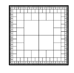
(a) Whitney decomposition of a square

(b) Polygonal arcs approximating $\partial R$

(c) Whitney squares separated from $\partial R$ by the arcs from 13(a)

(d) Triangulation of the region between the squares and $\partial R$

Figure 12. Illustration of the proof of Proposition 3.4

Let the $N\mathrel{\vbox{\hbox{\scriptsize.}\hbox{\scriptsize.}}}=\#P$ points of the partition be labelled as $x_{0},x_{1},\dots,x_{N}=x_{0}$ in positive orientation on $\partial R$, where $x_{0}=0$ is the lower left corner of $R$. Indices are considered modulo $N$. For each partition point $x_{k}$, set $D_{k}\mathrel{\vbox{\hbox{\scriptsize.}\hbox{\scriptsize.}}}=\min(|x_{k}-x_{k+1}|,|x_{k}-x_{k-1}|)$. By the bounded geometry assumption, we have $D_{k}\leq\lambda$ and

$$\frac{1}{\lambda}\leq\frac{D_{k}}{D_{k+1}}\leq\lambda.$$

In particular, $D_{k}/(8\lambda)\leq 1/8$, and so $D_{k}/(8\lambda)$ belongs to a dyadic interval of the form $(2^{-j-1},2^{-j}]$ for some $j\geq 3$. Let $d_{k}=\frac{3}{4}2^{-j}$ be the center of this interval. Note that $d_{k}$ and $D_{k}/(8\lambda)$ are comparable within a factor of $2$, so $d_{k}\leq D_{k}/(4\lambda)\leq\min(\frac{1}{4},D_{k}/4)$.

If $0=x_{0}<x_{1}<\dots<x_{n}=m$ are the partition points along the bottom edge of $R$ let $z_{k}=x_{k}+id_{k}$, $k=0,\dots,m$ and consider the polygonal arc $\sigma$ with these vertices. (See Figure 13(a).) Note that this arc connects the two vertical sides of $R$ and stays within $1/4$ of the bottom edge. Moreover, every segment has slope between $-1/4$ and $1/4$, since

$$\frac{\lvert d_{k}-d_{k+1}\rvert}{\lvert x_{k}-x_{k+1}\rvert}\leq\frac{\max(d_{k},d_{k+1})}{\lvert x_{k}-x_{k+1}\rvert}\leq\frac{1}{4}\cdot\frac{\max(D_{k},D_{k+1})}{\lvert x_{k}-x_{k+1}\rvert}\leq\frac{1}{4}.$$

Our choice of $d_{k}$ means that $z_{k}$ is at a height that is half way between the top and bottom edges of the dyadic square $Q$ that contains it. Since the segments of $\sigma$ have small slope, $\sigma$ leaves $Q$ near the two vertical side of $Q$ and this also holds for the dyadic squares to the left and right of $Q$.

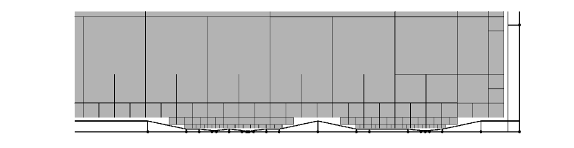
(a) The curves $\sigma$ and $\gamma$

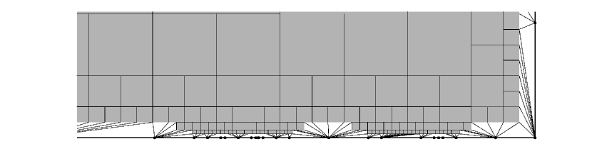
(b) Triangulating the region between $\gamma$ and $\partial R$

Figure 13. An enlargement of the curves $\sigma$ (small slopes) and $\gamma$ (axis parallel boundary of boxes). near the boundary. Above a partition point $x_{k}$ the curve $\gamma$ is parallel to the boundary on length comparable to $d_{k}$, and above each partition segment $\gamma$ is monotone (either it is flat or forms a steps that are all increasing or all decreasing). This makes it easy to verify that the region between $\gamma$ and $\partial R$ can be triangulated with a lower angle bound and without adding vertices to $\partial R$ or $\gamma$. In this picture the vertical scale is exaggerated to make $\sigma$ easier to see.

Making the same construction for each side we obtain four polygonal arcs $\sigma_{0},\dots,\sigma_{3}$, each approximating one side of the rectangle; see Figure 12(b). Consider a corner point of the rectangle, say $x_{0}=0$ to fix our ideas. The curves $\sigma_{0}$ and $\sigma_{3}$ reach the boundary at the points $id_{0}$ and $d_{0}$, respectively, and by the bounds on their slope, intersect in a single point within the dyadic square with centre $d_{0}+id_{0}$.

Now take the union of dyadic Whitney squares whose interiors do not hit the curves $\sigma_{j}$ and are separated from $\partial R$ by them (Figures 12(c) and 13(a)) This union is itself bounded by an axis-parallel polygon $\gamma$, which is the union of four polygonal arcs $\gamma_{0},\dots,\gamma_{3}$: The arc $\gamma_{0}$ begins at the upper right corner of the dyadic square centred at $d_{0}+id_{0}$ (which contains the intersection point $\sigma_{0}$ and $\sigma_{3}$), and ends similarly at the upper left corner of the square centred at $m-d_{n}+id_{n}$. (Recall that $x_{n}$ is the lower right corner of the rectangle. The arcs $\gamma_{1},\dots,\gamma_{2}$ are characterised similarly.

If we consider the polygonal arc $\sigma=\sigma_{0}$ corresponding to the bottom edge of $R$, then the portion of $\gamma_{0}$ above each partition arc $I$ is monotone and has a uniformly bounded number of vertices, depending only on $\lambda$. Because of the monotone property, all the vertices in the polygonal arc can be connected to the same endpoint of $I$ without hitting $\gamma$ and the angles between these connecting segments is bounded uniformly away from zero. (Figure 13(b).)

Moreover, for every partition point $x_{k}$ on the bottom edge, except the two corners, $\gamma_{0}$ is horizontal on some interval centered at $x_{k}$ and with length $\simeq d_{k}$; this is due to the property of $\sigma_{0}$ hitting only the vertical sides of dyadic squares near $x_{k}$. Therefore, connecting $x_{k}$ to the vertices of $\gamma_{0}$ whose projections are closest to $x_{k}$ to the right and left gives angles that are also bounded away from zero (as mentioned above, these two points belong to the same horizontal line). Do this for each side of the rectangle $R$. Finally, we connect each corner to the joint endpoint of the two corresponding $\gamma_{j}$; e.g., $0$ is connected to $4(d_{0}+id_{0})/3$.

Now every pair $x_{k}$ and $x_{k+1}$ is connected to a common vertex of $\gamma$, and likewise the two endpoints of every segment of $\gamma$ are connected to a common vertex of our partition. Thus we have triangulated the region between $\gamma$ and $\partial R$ by triangles whose angles are bounded away from zero. Any triangulation of the vertices of the Whitney squares also has angles bounded away from zero, and this proves the proposition. ∎

Remark.

The method described above actually produces a triangulation with $O(N)$ elements where $N$ is the number of partition points we start with. It is simple to implement in practice; Figures 13 and 12 were produced using such an implementation in MATLAB.

References

- [AR04] Venancio Álvarez and José M. Rodríguez, Structure theorems for Riemann and topological surfaces, J. London Math. Soc. (2) 69 (2004), no. 1, 153–168.
- [AR15] Omer Angel and Gourab Ray, Classification of half-planar maps, Ann. Probab. 43 (2015), no. 3, 1315–1349. MR 3342664
- [AS03] Omer Angel and Oded Schramm, Uniform infinite planar triangulations, Comm. Math. Phys. 241 (2003), no. 2-3, 191–213.
- [Ast94] Kari Astala, Area distortion of quasiconformal mappings, Acta Math. 173 (1994), no. 1, 37–60.
- [BCP19] Thomas Budzinski, Nicola Curien, and Bram Petri, The diameter of random Belyi surfaces, preprint, arXiv:1910.11809v1[math.GT], 2019.
- [BE19] Walter Bergweiler and Alexandre Eremenko, Quasiconformal surgery and linear differential equations, J. Anal. Math. 137 (2019), no. 2, 751–812.
- [Bel79] G. V. Belyĭ, Galois extensions of a maximal cyclotomic field, Izv. Akad. Nauk SSSR Ser. Mat. 43 (1979), no. 2, 267–276, 479.
- [Bel02] by same author, A new proof of the three-point theorem, Mat. Sb. 193 (2002), no. 3, 21–24. MR 1913596
- [Bis10] Christopher J. Bishop, Optimal angle bounds for quadrilateral meshes, Discrete Comput. Geom. 44 (2010), no. 2, 308–329.
- [Bis15] Christopher J. Bishop, Constructing entire functions by quasiconformal folding, Acta Mathematica 214 (2015), no. 1, 1–60.
- [BKKM86] D. V. Boulatov, V. A. Kazakov, I. K. Kostov, and A. A. Migdal, Analytical and numerical study of a model of dynamically triangulated random surfaces, Nuclear Phys. B 275 (1986), no. 4, 641–686.
- [BM04] Robert Brooks and Eran Makover, Random construction of Riemann surfaces, J. Differential Geom. 68 (2004), no. 1, 121–157. MR 2152911
- [BM17] Jérémie Bettinelli and Grégory Miermont, Compact Brownian surfaces I: Brownian disks, Probab. Theory Related Fields 167 (2017), no. 3-4, 555–614. MR 3627425
- [Boy55] B. V. Boyarskiĭ, Homeomorphic solutions of Beltrami systems, Dokl. Akad. Nauk SSSR (N.S.) 102 (1955), 661–664.
- [BS97] Philip L. Bowers and Kenneth Stephenson, A “regular” pentagonal tiling of the plane, Conform. Geom. Dyn. 1 (1997), 58–68.
- [BS17] by same author, Conformal tilings I: foundations, theory, and practice, Conform. Geom. Dyn. 21 (2017), 1–63.
- [BS19] by same author, Conformal tilings II: local isomorphism, hierarchy, and conformal type, Conform. Geom. Dyn. 23 (2019), 52–104.
- [Bud20] Thomas Budzinski, Infinite geodesics in hyperbolic random triangulations, Ann. Inst. Henri Poincaré Probab. Stat. 56 (2020), no. 2, 1129–1161. MR 4076778
- [CE18] Arnaud Chéritat and Adam Lawrence Epstein, Bounded type Siegel disks of finite type maps with few singular values, Sci. China Math. 61 (2018), no. 12, 2139–2156.
- [Cur16] Nicolas Curien, Planar stochastic hyperbolic triangulations, Probab. Theory Related Fields 165 (2016), no. 3-4, 509–540. MR 3520011
- [DR15] Francois David and Vincent Rohdes, Rémi Vargas, Liouville quantum gravity on the complex tori, preprint, arXiv:1501.00612v1 [math.PR].
- [EH95] A. Eremenko and D. H. Hamilton, On the area distortion by quasiconformal mappings, Proceedings of the American Mathematical Society 123 (1995), no. 9, 2793–2797.
- [Eps93] Adam Lawrence Epstein, Towers of finite type complex analytic maps, ProQuest LLC, Ann Arbor, MI, 1993, Thesis (Ph.D.)–City University of New York.
- [Ere04] A. Eremenko, Transcendental meromorphic functions with three singular values, Ill. J. Math. 48 (2004), no. 2, 701–709 (English).
- [FGJ15] Núria Fagella, Sébastian Godillon, and Xavier Jarque, Wandering domains for composition of entire functions, J. Math. Anal. Appl. 429 (2015), no. 1, 478–496.
- [For91] Otto Forster, Lectures on Riemann surfaces, Graduate Texts in Mathematics, vol. 81, Springer-Verlag, New York, 1991, Translated from the 1977 German original by Bruce Gilligan, Reprint of the 1981 English translation.
- [Fre73] Hans Freudenthal, Kerékjártó, Béla, Dictionary of Scientific Biography, Volume VII, 1973.
- [Gar84] Frederick P. Gardiner, Approximation of infinite-dimensional Teichmüller spaces, Trans. Amer. Math. Soc. 282 (1984), no. 1, 367–383.
- [GN67] R. C. Gunning and Raghavan Narasimhan, Immersion of open Riemann surfaces, Math. Ann. 174 (1967), 103–108.
- [GO08] Anatoly A. Goldberg and Iossif V. Ostrovskii, Value distribution of meromorphic functions. Transl. from the Russian by Mikhail Ostrovskii. With an appendix by Alexandre Eremenko and James K. Langley, vol. 236, Providence, RI: American Mathematical Society (AMS), 2008 (English).
- [GR66] F. W. Gehring and E. Reich, Area distortion under quasiconformal mappings, Ann. Acad. Sci. Fenn. Ser. A I No. 388 (1966), 15. MR 0201635
- [Gro97] Alexandre Grothendieck, Esquisse d’un programme, Geometric Galois actions, 1, London Math. Soc. Lecture Note Ser., vol. 242, Cambridge Univ. Press, Cambridge, 1997, With an English translation on pp. 243–283, pp. 5–48.
- [Hub06] John Hamal Hubbard, Teichmüller theory and applications to geometry, topology, and dynamics. Vol. 1, Matrix Editions, Ithaca, NY, 2006, Teichmüller theory, With contributions by Adrien Douady, William Dunbar, Roland Roeder, Sylvain Bonnot, David Brown, Allen Hatcher, Chris Hruska and Sudeb Mitra, With forewords by William Thurston and Clifford Earle.
- [JW16] Gareth A. Jones and Jürgen Wolfart, Dessins d’enfants on Riemann surfaces, Springer Monographs in Mathematics, Springer, Cham, 2016.
- [KPT15] Jeremy Kahn, Kevin M. Pilgrim, and Dylan P. Thurston, Conformal surface embeddings and extremal length, arXiv e-prints (2015), arXiv:1507.05294.
- [Lan02] James K. Langley, Critical values of slowly growing meromorphic functions, Comput. Methods Funct. Theory 2 (2002), no. 2, 539–547 (English).
- [Laz17] Kirill Lazebnik, Several constructions in the Eremenko-Lyubich class, J. Math. Anal. Appl. 448 (2017), no. 1, 611–632.
- [Lef25] S. Lefschetz, Book review: Kerékjártó, Vorlesungen über Topologie. i. flächentopologie, Bull. Amer. Math. Soc. 31 (1925), 176.
- [Leh87] Olli Lehto, Univalent functions and Teichmüller spaces, Graduate Texts in Mathematics, vol. 109, Springer-Verlag, New York, 1987.
- [LG07] Jean-François Le Gall, The topological structure of scaling limits of large planar maps, Invent. Math. 169 (2007), no. 3, 621–670. MR 2336042
- [LG19] by same author, Brownian geometry, Jpn. J. Math. 14 (2019), no. 2, 135–174. MR 4007665
- [LV73] O. Lehto and K. I. Virtanen, Quasiconformal mappings in the plane, second ed., Springer-Verlag, New York-Heidelberg, 1973, Translated from the German by K. W. Lucas, Die Grundlehren der mathematischen Wissenschaften, Band 126.
- [LZ04] Sergei K. Lando and Alexander K. Zvonkin, Graphs on surfaces and their applications, Encyclopaedia of Mathematical Sciences, vol. 141, Springer-Verlag, Berlin, 2004, With an appendix by Don B. Zagier, Low-Dimensional Topology, II.
- [Mar13] J. Martel, Belyi functions on non-compact surfaces; or: Building Riemann surfaces from equilateral triangles, MathOverflow, 2013, URL:https://mathoverflow.net/q/146503 (version: 2013-10-31).
- [Mie14] Grégory Miermont, Aspects of random maps, Lecture notes of the 2014 Saint-Flour Probability Summer School.
- [Mil06] John Milnor, Dynamics in one complex variable, third ed., Annals of Mathematics Studies, vol. 160, Princeton University Press, Princeton, NJ, 2006. MR 2193309
- [Mir13] Maryam Mirzakhani, Growth of Weil-Petersson volumes and random hyperbolic surfaces of large genus, J. Differential Geom. 94 (2013), no. 2, 267–300. MR 3080483
- [MPS20] David Martí-Pete and Mitsuhiro Shishikura, Wandering domains for entire functions of finite order in the Eremenko-Lyubich class, Proc. Lond. Math. Soc. (3) 120 (2020), no. 2, 155–191.
- [MS16a] Jason Miller and Scott Sheffield, Liouville quantum gravity and the Brownian map II: Geodesics and continuity of the embedding, Preprint, arXiv:1605.03563.
- [MS16b] by same author, Liouville quantum gravity and the Brownian map III: the conformal structure is determined, Preprint, arXiv:1608.05391.
- [MS20] by same author, Liouville quantum gravity and the Brownian map I: the metric, Invent. Math. 219 (2020), no. 1, 75–152. MR 4050102
- [OS16] John W. Osborne and David J. Sixsmith, On the set where the iterates of an entire function are neither escaping nor bounded, Ann. Acad. Sci. Fenn. Math. 41 (2016), no. 2, 561–578.
- [Rad25] T. Radó, Über den Begriff der Riemannschen Fläche., Acta Litt. Sci. Szeged 2 (1925), 101–121 (German).
- [Rem09] Lasse Rempe, Hyperbolic dimension and radial Julia sets of transcendental functions, Proc. Amer. Math. Soc. 137 (2009), no. 4, 1411–1420.
- [Rem16] Lasse Rempe, Arc-like continua, Julia sets of entire functions, and Eremenko’s Conjecture, 2016.
- [Ric63] Ian Richards, On the classification of noncompact surfaces, Trans. Amer. Math. Soc. 106 (1963), 259–269. MR 0143186
- [Sch94] Leila Schneps (ed.), The Grothendieck theory of dessins d’enfants, London Mathematical Society Lecture Note Series, vol. 200, Cambridge University Press, Cambridge, 1994, Papers from the Conference on Dessins d’Enfant held in Luminy, April 19–24, 1993.
- [vK23] B. von Kerékjártó, Vorlesungen über Topologie. I.: Flächentopologie. Mit 80 Textfiguren., vol. 8, Springer, Berlin, 1923 (German).
- [VS89] V. A. Voevodskiĭ and G. B. Shabat, Equilateral triangulations of Riemann surfaces, and curves over algebraic number fields, Dokl. Akad. Nauk SSSR 304 (1989), no. 2, 265–268.
- [Wil03] G. Brock Williams, Noncompact surfaces are packable, J. Anal. Math. 90 (2003), 243–255.
- [Wit55] Hans Wittich, Neuere Untersuchungen über eindeutige analytische Funktionen, vol. 8, Springer-Verlag, Berlin, 1955 (German).