Robust finite element error estimates for elliptic and parabolic distributed optimal control problems
with energy regularization

Space-time finite element methods for the initial temperature reconstruction

Abstract

This work is devoted to the reconstruction of the initial temperature in the backward heat equation using the space-time finite element method on fully unstructured space-time simplicial meshes proposed by Steinbach (2015). Such a severely ill-posed problem is tackled by the standard Tikhonov regularization method. This leads to a related optimal control for an parabolic equation in the space-time domain. In this setting, the control is taken as initial condition, whereas the terminal observation data serve as target. The objective becomes a standard terminal observation functional combined with the Tikhonov regularization. The space-time finite element method is applied to the space-time optimality system that is well-posed for a fixed regularization parameter.

1 Introduction

In this work, we investigate the applicability of unstructured space-time methods to the numerical solution of inverse problems using the classical inverse problem of the reconstruction of the initial temperature in the heat equation from an observation of the temperature at a finite time horizon: Find the initial temperature $u_{0}(\cdot):=u(\cdot,0)\in L^{2}(\Omega)$ on $\Sigma_{0}$ such that

$$\partial_{t}u-\Delta_{x}u=0\quad\mbox{in}\;Q,\quad u=0\quad\mbox{on}\;\Sigma,\quad u=u_{T}^{\delta}\quad\mbox{on}\;\Sigma_{T}\,,$$ (1)

where $Q:=\Omega\times(0,T)$ denotes the space-time cylinder with the boundary $\partial Q=\overline{\Sigma}\cup\overline{\Sigma}_{0}\cup\overline{\Sigma}_{T}$, $\Sigma:=\partial\Omega\times(0,T)$, $\Sigma_{0}:=\Omega\times\{0\}$, $\Sigma_{T}:=\Omega\times{T}$, the bounded Lipschitz domain $\Omega\subset{\mathbb{R}}^{d}$, $d\in\{1,2,3\}$, and a finite time horizon $T>0$. Moreover, $u_{T}^{\delta}\in L^{2}(\Omega)$ denotes the observed terminal temperature which may contain some noise characterized by the noise level $\delta\geq 0$,

$$\|u_{T}^{\delta}-u_{T}\|_{L^{2}(\Omega)}\leq\delta,$$ (2)

where $u_{T}=u(\cdot,T)\in L^{2}(\Omega)$ represents the unpolluted exact data.

In contrast to the forward heat equation with known initial data, the backward heat equation (1) is severely ill-posed; see [2, Example 2.9]. In fact, the solution of (1) does not continuously depend on the data $u_{T}^{\delta}$ even when the solution exists. Following the notation in [2], the problem (1) may be reformulated as an abstract operator equation in a more general setting: Find $u_{0}\in{\mathcal{X}}$ such that

$$Su_{0}=u_{T},$$ (3)

where $S:{\mathcal{X}}\rightarrow{\mathcal{Y}}$ denotes a bounded linear operator between two Hilbert spaces ${\mathcal{X}}$ and ${\mathcal{Y}}$. It is clear that there does not exist a continuous inverse operator $S^{-1}:{\mathcal{Y}}\rightarrow{\mathcal{X}}$ in general. Therefore, we consider a regularized solution, depending on the choice of Tikhonov’s regularization parameter $\varrho:=\varrho(\delta)$,

$$u_{0}^{\delta,\varrho}:=\left(S^{*}S+\varrho I\right)^{-1}S^{*}u_{T}^{\delta},$$

as the unique minimizer of the Tikhonov functional [9]

$${\mathcal{J}}_{\varrho}(z):=\frac{1}{2}\,\|Sz-u_{T}^{\delta}\|_{\mathcal{Y}}+\frac{\varrho}{2}\,\|z\|^{2}_{\mathcal{X}}.$$ (4)

It is well known that we have the convergence

$$\lim_{\delta\rightarrow 0}u_{0}^{\delta,\varrho}=u_{0}^{\dagger}{\text{ in }{\mathcal{X}},}\text{ if the conditions}\;\;\lim\limits_{\delta\rightarrow 0}\varrho(\delta)=0\;\;\mbox{and}\;\lim_{\delta\rightarrow 0}\frac{\delta^{2}}{\varrho(\delta)}=0$$

are satisfied. Here, $u_{0}^{\dagger}$ denotes the best-approximated solution to the operator equation (3); see [2, Theorem 5.2] for a more detailed discussion, and also [1, 7].

The main focus of this work is to describe a space-time finite element method (FEM) on fully unstructured simplicial meshes to solve the minimization problem (4) subject to the solution of the heat equation (1). Such a space-time method has been studied for the forward heat equation in [8], and for other parabolic optimal control problems in [5, 6].

The remainder of this paper is structured as follows: In Section 2, we discuss the related optimal control problem. Its solution is obtained by the optimality system consisting of the (forward) heat equation, the adjoint heat equation, and the gradient equation. Based on the Banach–Nečas–Babuška theory [3], we establish unique solvability of the resulting coupled system, when eliminating the unknown initial datum. In Section 3, for the numerical solution of the inverse problem (1), we first consider the discrete optimal control problem, which is based on the space-time discretization of the forward problem. The solution is characterized by a discrete gradient equation, which turns out to be the Schur complement system of the discretized coupled variational formulation. First numerical results are reported in Section 4. These results show the potential of the space-time approach proposed. Finally, some conclusions are drawn in Section 5.

2 The related optimal control problem

In our case, the Hilbert spaces ${\mathcal{X}}$ and ${\mathcal{Y}}$ are specified as ${\mathcal{X}}={\mathcal{Y}}=L^{2}(\Omega)$, and the image $Sz$ of the operator $S:L^{2}(\Omega)\to L^{2}(\Omega)$ in the Tikhonov functional (4) is defined by the solution $u\in X:=L^{2}(0,T;H_{0}^{1}(\Omega))\cap H^{1}(0,T;H^{-1}(\Omega))$ of the forward heat conduction problem

$$\partial_{t}u-\Delta_{x}u=0\quad\mbox{in}\;Q,\quad u=0\quad\mbox{on}\;\Sigma,\quad u=z\quad\mbox{on}\;\Sigma_{0},$$ (5)

and its evaluation on $\Sigma_{T}$, i.e., $(Sz)(x)=u(x,T)$, $x\in\Omega$. Here, the control $z\in L^{2}(\Omega)$ represents the initial data in (5). Rewriting the minimization of the functional (4) in terms of $z$, we obtain the optimal control problem

$${\mathcal{J}}_{\varrho}(z):=\frac{1}{2}\,\|u(x,T)-u_{T}^{\delta}\|^{2}_{L^{2}(\Omega)}+\frac{\varrho}{2}\,\|z\|^{2}_{L^{2}(\Omega)}\to\min_{z\in L^{2}(\Omega)},$$ (6)

where the state $u\in X$ is associated to the control $z$ subject to (5).

To set up the necessary and sufficient optimality conditions for the optimal control $z$ with associated state $u$, we introduce the adjoint equation

$$-\partial_{t}p-\Delta_{x}p=0\quad\mbox{in}\;Q,\quad p=0\quad\mbox{on}\;\Sigma,\quad p=u-u_{T}^{\delta}\quad\mbox{on}\;\Sigma_{T}.$$ (7)

It has a unique solution $p\in X$, the adjoint state. The adjoint equation can be derived by a formal Lagrangian technique as in [10]. If $z$ is the optimal control with associated state $u\in X$, then a unique adjoint state $p\in X$ solving (7) exists such that the gradient equation

$$p+\varrho\,z=0\quad\textup{on }\Sigma_{0}$$ (8)

is satisfied. Using this equation, we can eliminate the unknown initial datum $z$ in the state equation (5) to conclude

$$\partial_{t}u-\Delta_{x}u=0\quad\mbox{in}\;Q,\quad u=0\quad\mbox{on}\;\Sigma,\quad u=-\frac{1}{\varrho}\,p\quad\mbox{on}\;\Sigma_{0}$$ (9)

for the optimal state $u$. The reduced optimality system (7),(9) is necessary and sufficient for optimality of $u$ with associated adjoint state $p$. In what follows, we will describe a space-time finite element approximation of this system.

The space-time variational formulation of the heat equation in (9) (without initial condition) is to find $u\in X$ such that

$$b(u,v):=\int_{0}^{T}\int_{\Omega}\Big{[}\partial_{t}u(x,t)v(x,t)+\nabla_{x}u(x,t)\cdot\nabla_{x}v(x,t)\Big{]}\,dx\,dt=0$$ (10)

is satisfied for all $v\in Y:=L^{2}(0,T;H_{0}^{1}(\Omega))$. The spaces $X$ and $Y$ are equipped with the norms

$$\|v\|_{Y}=\|\nabla_{x}v\|_{L^{2}(Q)}\;\;\mbox{and}\;\;\|u\|_{X}=\sqrt{\|\partial_{t}u\|_{Y^{*}}^{2}+\|u\|_{Y}^{2}}=\sqrt{\|w_{u}\|_{Y}^{2}+\|u\|_{Y}^{2}},$$

with $w_{u}\in Y$ being the unique solution of the variational problem

$$\int_{0}^{T}\int_{\Omega}\nabla_{x}w_{u}(x,t)\cdot\nabla_{x}v(x,t)\,dx\,dt=\int_{0}^{T}\int_{\Omega}\partial_{t}u(x,t)\,v(x,t)\,dx\,dt\quad\forall\,v\in Y.$$

We multiply the adjoint heat equation (7) by a test function $q\in X$, integrate over $Q$, and apply integration by parts both in space and time. Then we insert the terminal data $u(T)-u_{T}^{\delta}$ of $p$ in the arising term $p(T)$, and substitute the term $p(0)$ by $-\rho z=-\rho u(0)$ in view of (8). In this way, we arrive at the weak form of the adjoint problem (7)

$$0 = \int_{0}^{T}\int_{\Omega}\Big{[}-\partial_{t}p(x,t)\,q(x,t)-\Delta_{x}p(x,t)\,q(x,t)\Big{]}dx\,dt$$

$$= -\int_{\Omega}[u(x,T)-u^{\delta}_{T}(x)]\,q(x,T)\,dx-\varrho\int_{\Omega}u(x,0)\,q(x,0)\,dx$$

$$\hskip 28.45274pt+\int_{0}^{T}\int_{\Omega}\Big{[}p(x,t)\,\partial_{t}q(x,t)+\nabla_{x}p(x,t)\cdot\nabla_{x}q(x,t)\Big{]}dx\,dt\,.$$

We end up with the variational problem to find $(u,p)\in X\times Y$ such that

$${\mathcal{B}}(u,p;v,q)=\langle u_{T}^{\delta},q(T)\rangle_{L^{2}(\Omega)}\quad\forall\,(v,q)\in Y\times X,$$ (11)

where the bilinear form ${\mathcal{B}}(\cdot,\cdot;\cdot,\cdot)$ is given as

$${\mathcal{B}}(u,p;v,q):=b(u,v)-b(q,p)+\langle u(T),q(T)\rangle_{L^{2}(\Omega)}+\varrho\,\langle u(0),q(0)\rangle_{L^{2}(\Omega)}\,.$$

We note that the bilinear form $b(\cdot,\cdot)$, as defined by (10), is bounded:

$$|b(u,v)|\leq\sqrt{2}\,\|u\|_{X}\|v\|_{Y}\quad\forall\,u\in X,v\in Y.$$

For $u\in X$ we have $\|u(0)\|_{L^{2}(\Omega)}\leq\mu\,\|u\|_{X}$ and $\|u(T)\|_{L^{2}(\Omega)}\leq\mu\,\|u\|_{X}$ with

$$\mu:=\left(1+\frac{1}{2}\left[\frac{c_{F}}{T}\right]^{2}+\sqrt{\frac{1}{4}\left[\frac{c_{F}}{T}\right]^{4}+\left[\frac{c_{F}}{T}\right]^{2}}\right)^{1/2},$$

where $c_{F}$ is the constant in Friedrichs’ inequality in $H_{0}^{1}(\Omega)$. With these ingredients, we are in the position to prove that the bilinear form ${\mathcal{B}}(\cdot,\cdot;\cdot,\cdot)$ is bounded, i.e., for all $(u,p),(q,v)\in X\times Y$, there holds

$$|{\mathcal{B}}(u,p;v,q)|\,\leq\,2\,(1+\varrho)\,\mu^{2}\,\sqrt{\|u\|_{X}^{2}+\|p\|_{Y}^{2}}\,\sqrt{\|q\|_{X}^{2}+\|v\|_{Y}^{2}}\,.$$

Moreover, we can establish the following inf-sup stability condition which can be proved similarly to [5, Lemma 3.2].

Lemma 1.

For simplicity, let us assume $\varrho\in(0,1]$. Then there holds the inf-sup stability condition

$$\frac{3}{10}\,\varrho\,\sqrt{\|u\|_{X}^{2}+\|p\|_{Y}^{2}}\leq\sup\limits_{0\neq(v,q)\in Y\times X}\frac{{\mathcal{B}}(u,p;v,q)}{\sqrt{\|q\|_{X}^{2}+\|v\|_{Y}^{2}}}\quad\forall\,(u,p)\in X\times Y.$$

Moreover, for all $(v,q)\in Y\times X$, there exist $(\overline{u},\overline{p})\in X\times Y$ satisfying

$${\mathcal{B}}(\overline{u},\overline{p};v,q)>0.$$

Now, using the Banach–Nečas–Babuška theorem (see, e.g., [3]), we can ensure well-posedness of the variational optimality problem (11) for any fixed positive regularization parameter $\varrho$.

3 Space-time finite element methods

For the space-time finite element discretization of the variational formulation (11), we first introduce conforming finite element spaces $X_{h}\subset X$ and $Y_{h}\subset Y$. In particular, we consider $X_{h}=Y_{h}$ spanned by piecewise linear continuous basis functions which are defined with respect to some admissible decomposition of the space-time domain $Q$ into shape regular simplicial finite elements. In addition, we will use the subspace $Y_{0,h}\subset Y_{h}$ of basis functions with zero initial values. Moreover, $Z_{h}\subset L^{2}(\Omega)$ is a finite element space to discretize the control $z$. The space-time finite element discretization of the forward problem (5) reads to find $u_{h}\in X_{h}$ such that

$$b(u_{h},v_{h})=0\quad\forall v_{h}\in Y_{0,h},\quad\langle u_{h}-z_{h},v_{h}\rangle_{L^{2}(\Sigma_{0})}=0\quad\forall v_{h}\in Y_{h}\backslash Y_{0,h}.$$ (12)

When denoting the degrees of freedom of $u_{h}$ at $\Sigma_{0}$, at $\Sigma_{T}$, and in $Q$ by $\underline{u}_{0}$, $\underline{u}_{T}$, and $\underline{u}_{I}$, respectively, the variational formulation (12) is equivalent to the linear system

$$\left(\begin{array}[]{ccc}M_{00}&&\\ K_{0I}&K_{II}&K_{TI}\\ &K_{IT}&K_{TT}\end{array}\right)\left(\begin{array}[]{c}\underline{u}_{0}\\ \underline{u}_{I}\\ \underline{u}_{T}\end{array}\right)=\left(\begin{array}[]{c}M_{h}^{\top}\underline{z}\\ \underline{0}\\ \underline{0}\end{array}\right),$$

where the block entries of the stiffness matrix $K_{h}$ and the mass matrices $M_{00}$ and $M_{h}$ are defined accordingly. After eliminating $\underline{u}_{0}$, the resulting system corresponds to the space-time finite element approach as considered in [8]. In particular, we can compute $\underline{u}_{T}=A_{h}\underline{z}$ to determine $u_{h}(T)$ in dependency on the initial datum $z_{h}$, where

$$A_{h}=\Big{(}K_{TT}-K_{IT}K_{II}^{-1}K_{TI}\Big{)}^{-1}K_{IT}K_{II}^{-1}K_{0I}M_{00}^{-1}M_{h}^{\top}=\widetilde{A}_{h}M_{h}^{\top}\,.$$

Instead of the cost functional (6), we now consider the discrete cost functional

$${\mathcal{J}}_{\varrho,h}(z_{h}) = \frac{1}{2}\,\|u_{h}(x,T)-u_{T}^{\delta}\|^{2}_{L^{2}(\Omega)}+\frac{\varrho}{2}\,\|z_{h}\|^{2}_{L^{2}(\Omega)}$$

$$= \frac{1}{2}\,(A_{h}^{\top}M_{TT}A_{h}\underline{z},\underline{z})-(A_{h}^{\top}\underline{f},\underline{z})+\frac{1}{2}\,\|u_{T}^{\delta}\|^{2}_{L^{2}(\Omega)}+\frac{\varrho}{2}\,(\overline{M}_{h}\underline{z},\underline{z}),$$

whose minimizer is given as the solution of the linear system

$$A_{h}^{\top}(M_{TT}A_{h}\underline{z}-\underline{f})+\varrho\,\overline{M}_{h}\underline{z}=\underline{0}.$$ (13)

Note that $M_{TT}$ is the mass matrix formed by the basis functions of $X_{h}$ at $\Sigma_{T}$, $\overline{M}_{h}$ is the mass matrix related to the control space $Z_{h}$, and $\underline{f}$ is the load vector of the target $u_{T}^{\delta}$ tested with basis functions from $X_{h}$ at $\Sigma_{T}$. When inserting $\underline{u}_{T}=A_{h}\underline{z}$ and introducing $\underline{p}_{0}:=\widetilde{A}_{h}^{\top}(M_{TT}\underline{u}_{T}-\underline{f})$, $\underline{p}_{T}:=(K_{TT}-K_{IT}K_{II}^{-1}K_{TI})^{-\top}(M_{TT}\underline{u}_{T}-\underline{f})$, $\underline{p}_{I}:=-K_{II}^{-\top}K_{IT}^{\top}\underline{p}_{T}$, this finally results in the linear system to be solved:

$$\left(\begin{array}[]{ccccccc}&&&&-M_{00}&-K_{0I}^{\top}&\\ &&&&&-K_{II}^{\top}&-K_{IT}^{\top}\\ &&M_{TT}&&&-K_{TI}^{\top}&-K_{TT}^{\top}\\ &&&\varrho\overline{M}_{h}&M_{h}&&\\ M_{00}&&&-M_{h}^{\top}&&&\\ K_{0I}&K_{II}&K_{TI}&&&&\\ &K_{IT}&K_{TT}&&&&\end{array}\right)\left(\begin{array}[]{c}\underline{u}_{0}\\ \underline{u}_{I}\\ \underline{u}_{T}\\ \underline{z}\\ \underline{p}_{0}\\ \underline{p}_{I}\\ \underline{p}_{T}\end{array}\right)=\left(\begin{array}[]{c}\underline{0}\\ \underline{0}\\ \underline{f}\\ \underline{0}\\ \underline{0}\\ \underline{0}\\ \underline{0}\end{array}\right).$$ (14)

In the particular case, when $Z_{h}=Y_{h|\Sigma_{0}}\subset H^{1}_{0}(\Omega)$ is the space of piecewise linear basis functions as well, the mass matrices $M_{00}=\overline{M}_{h}=M_{h}$ coincide, and therefore we can eliminate $\underline{z}=\underline{u}_{0}$ and $\underline{p}_{0}=-\varrho\underline{z}=-\varrho\underline{u}_{0}$ to obtain

$$\left(\begin{array}[]{ccccc}\varrho M_{00}&&&-K_{0I}^{\top}&\\ &&&-K_{II}^{\top}&-K_{IT}^{\top}\\ &&M_{TT}&-K_{TI}^{\top}&-K_{TT}^{\top}\\ K_{0I}&K_{II}&K_{TI}&&\\ &K_{IT}&K_{TT}&&\\ \end{array}\right)\left(\begin{array}[]{c}\underline{u}_{0}\\ \underline{u}_{I}\\ \underline{u}_{T}\\ \underline{p}_{I}\\ \underline{p}_{T}\end{array}\right)=\left(\begin{array}[]{c}\underline{0}\\ \underline{0}\\ \underline{f}\\ \underline{0}\\ \underline{0}\end{array}\right).$$ (15)

Note that (15) is nothing but the Galerkin discretization of the variational formulation (11) when using $X_{h}\subset X$ and $Y_{0,h}\subset Y$ as finite element ansatz and test spaces. Obviously, the linear system (13) and, therefore, (15) are uniquely solvable.

In practice, the noise level $\delta\geq 0$ is usually given by the measurement environment, and one has to choose suitable discretization and regularization parameters $h$ and $\rho$. This is well investigated for linear inverse problems; see, e.g., the classical book by Tikhonov and Arsenin [9] and the more recent publications [2, 4]. In our numerical experiments presented in the next section, we only play with the parmeters $\delta$ and $h$ for a fixed small $\varrho$.

4 Numerical results

We take $\Omega=(0,1)$ and $T=1$, i.e., $Q=(0,1)^{2}$, and consider the manufactured observation data $u_{T}^{\delta}(x):=e^{-\pi^{2}}\sin(\pi x)+\delta\sin(10\pi x)$ with some noise represented by the second term; see exact and noisy data with $\delta\in\{0,10^{-5},5\cdot 10^{-6},2.5\cdot 10^{-6}\}$ in Fig. 1.

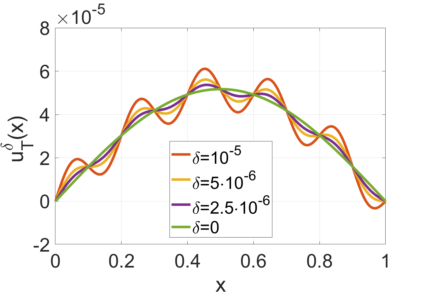
Figure 1: Comparison of the exact ($\delta=0$) and noisy ($\delta>0$) observation data.

To study the convergence of the space-time finite element solution to the exact initial datum, we use the target $u_{T}(x)=e^{-\pi^{2}}\sin(\pi x)$ without any noise. The reconstructed initial data with respect to a varying mesh size are illustrated in the left plot of Fig. 2, where $\varrho=10^{-14}$. We clearly see the convergence of the approximations to the exact initial datum with respect to the mesh refinement. The right plot of Fig. 2 shows the reconstructed initial approximation with different noise levels $\delta$. For a decreasing $\delta$, we observe an improved reconstruction.

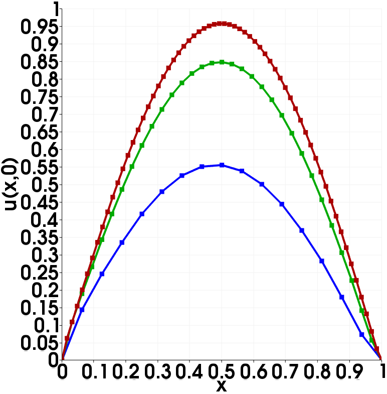
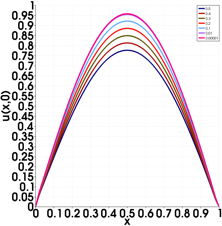
Figure 2: Convergence of the reconstructed initial data with respect to the mesh refinement $h\in\{1/16,1/32,1/64\}$, $\delta=0$, $\varrho=10^{-14}$ (left), and convergence with respect to the noise level $\delta\in\{0.5,0.4,0.3,0.2,10^{-1},10^{-3},10^{-5}\}$, $h=1/64$, $\varrho=10^{-14}$ (right).

5 Conclusions

We have applied the space-time FEM from [8] to the numerical solution of the classical inverse heat conduction problem to determine the initial datum from measured observation data at some time horizon $T$. The numerical results show the potential of this approach for more interesting inverse problems. The space-time FEM are very much suited for designing smart adaptive algorithms along the line proposed in [4] determining the optimal choice of $\varrho$ and $h$ for a given noise level $\delta$ in a multilevel (nested iteration) setting.

References

- [1] D.-H. Chen, B. Hofmann, and J. Zou. Regularization and convergence for ill-posed backward evolution equations in Banach spaces. J. Differential Equations, 265:3533–3566, 2018.
- [2] H. W. Engl, M. Hanke, and G. Neubauer. Regularization of Inverse Problems. Springer Netherlands, 1996.
- [3] A. Ern and J.-L. Guermond. Theory and Practice of Finite Elements. Springer, New York, 2004.
- [4] A. Griesbaum, B. Kaltenbacher, and B. Vexler. Efficient computation of the Tikhonov regularization parameter by goal-oriented adaptive discretization. Inverse Problems, 24:025025 (20pp.), 2008.
- [5] U. Langer, O. Steinbach, F. Tröltzsch, and H. Yang. Space-time finite element discretization of parabolic optimal control problems with energy regularization. SIAM J. Numer. Anal., 59:675–695, 2021.
- [6] U. Langer, O. Steinbach, F. Tröltzsch, and H. Yang. Unstructured space-time finite element methods for optimal control of parabolic equations. SIAM J. Sci. Comput., 43:A744–A771, 2021.
- [7] D. Leykekhman, B. Vexler, and D. Walter. Numerical analysis of sparse initial data identification for parabolic problems. ESAIM Math. Model. Numer. Anal., 54:1139–1180, 2020.
- [8] O. Steinbach. Space-time finite element methods for parabolic problems. Comput. Methods Appl. Math., 15(4):551–566, 2015.
- [9] A. N. Tikhonov and V. Y. Arsenin. Solution of Ill-posed Problems. Winston & Sons, Washington, 1977.
- [10] F. Tröltzsch. Optimal control of partial differential equations: Theory, methods and applications, volume 112 of Graduate Studies in Mathematics. American Mathematical Society, Providence, Rhode Island, 2010.