Observations of the Quiet Sun During the Deepest Solar Minimum of the Past Century with Chandrayaan-2 XSM – Sub-A Class Microflares Outside Active Regions

Abstract

Solar flares, with energies ranging over several orders of magnitude, result from impulsive release of energy due to magnetic reconnection in the corona. Barring a handful, almost all microflares observed in X-rays are associated with the solar active regions. Here we present, for the first time, a comprehensive analysis of a large sample of quiet Sun microflares observed in soft X-rays by the Solar X-ray Monitor (XSM) on board the Chandrayaan-2 mission during the 2019-20 solar minimum. A total of 98 microflares having peak flux below GOES A-level were observed by the XSM during observations spanning 76 days. By using the derived plasma temperature and emission measure of these events obtained by fitting the XSM spectra along with volume estimates from concurrent imaging observations in EUV with the Solar Dynamics Observatory/Atmospheric Imaging Assembly (SDO-AIA), we estimated their thermal energies to be ranging from $3\times 10^{26}$ to $6\times 10^{27}$ erg. We present the frequency distribution of the quiet Sun microflares with energy and discuss the implications of these observations of small scale magnetic reconnection events outside active regions on coronal heating.

1 Introduction

Explaining the million Kelvin hot corona over a relatively cooler ($\sim$6000 K) solar photosphere is one of the long-standing problems of astrophysics. It is fairly well accepted that the magnetic field plays a crucial role in transporting energy from within the Sun to its atmosphere. However, there is no conclusive evidence, yet, to explain the mechanism involved in the process. Two widely considered mechanisms that can heat the corona are heating by Magnetohydrodynamic (MHD) waves and magnetic reconnection (Klimchuk, 2006).

The large solar flares, which occur due to magnetic reconnection and release total energy ranging from $10^{30}$ to $10^{33}$ erg, can only account for 20% of the overall coronal energy requirement (Sakurai, 2017). It is known that the solar flares follow a power law distribution and thus the smaller flares occur more frequently, suggesting that even smaller flares may fulfill the energy demand of coronal heating. Based on the early observations of microflares from the Sun (e.g., Lin et al., 1984), Parker (1988) hypothesized that the solar corona is heated by the small scale reconnection events, termed as nanoflares having total energy around $\sim 10^{24}$ erg, occurring all over the Sun. Since observations of individual small scale reconnection events have not been possible so far due to technological limitations, one possible way to infer their frequency is by extrapolating the power law of the observable microflare distribution to lower energies. However,  Hudson (1991) showed that for the small scale events to be dominant over the large solar flares, the power law index should be greater than two. Thus, it is of great importance to constrain the power law index of the flare frequency distribution from the observations of microflares in order to confirm the nanoflare hypothesis.

Several efforts have been made to obtain the frequency distribution of microflares using observations at different wavelengths. In X-rays, the first statistical study of microflares was carried out using the Yokoh Soft X-ray Telescope (SXT), where an active region was observed for five days. Total energy of the microflares observed during this period was inferred from the temperature and emission measure determined using images from two different filters (Shimizu, 1995) to obtain the frequency distribution within the energy range of $10^{26}$ to $10^{28}$ erg. The most comprehensive statistical study of microflares was carried out using the Reuven Ramaty High Energy Solar Spectroscopic Imager (RHESSI) observatory in hard X-ray. This study, spanning over five years (Christe et al., 2008; Hannah et al., 2008) reported more than 25000 microflares, having energies of the order of $10^{27}$erg or higher. The flare parameters were obtained by modeling the X-ray spectrum. It should be noted that both the statistical studies were limited to X-ray microflares occuring within active regions.

On the other hand, the proposed nanoflares responsible for heating the corona are expected to be present everywhere on the solar disk, including the quiet corona outside active regions. There have been reports of observations small burst like events in EUV with SOHO EIT (Krucker & Benz, 1998; Benz & Krucker, 2002) and TRACE (Aschwanden et al., 2000b; Parnell & Jupp, 2000), with total thermal energy in the range of $10^{24}-10^{26}$erg and following the expected power law distribution. However, it is not clear whether all these events do reach up to coronal temperature or not, due to the difficulties in discriminating impulsive heating events from other brightenings in the EUV wavebands (Aschwanden et al., 2000a, b). While this ambiguity does not arise at X-ray energies where the emission arises from higher temperature plasma, there are very few observations due to the technical limitations involved. There have been only a handful of X-ray microflares detected in the quiet Sun with Yokoh SXT (Krucker et al., 1997), SphinX (Sylwester et al., 2019), and NuSTAR (Kuhar et al., 2018). Hence, no statistical studies of quiet Sun X-ray microflares have been possible so far.

The Solar X-ray Monitor (XSM)  (Vadawale et al., 2014; Shanmugam et al., 2020) on board the Chandrayaan-2 mission observed a large number of microflares in the quiet Sun. XSM provides disk integrated X-ray spectral measurements of the Sun with sensitivities down to sub-A class X-ray activity (Mithun et al., 2020). It carried out observations of the Sun during 2019-20 solar minimum, which was the deepest in the past 100 years (Janardhan et al., 2011, 2015), when there were extended periods without any active regions present on the solar disk, providing a unique opportunity to observe these microflares in the quiet Sun. Spectroscopic investigation of non-flaring quiescent corona during this period is discussed in a companion paper  (hereafter paper-I). Here, we present a detailed study of microflares occurring outside active regions as observed by the XSM during this period. Rest of the paper is organized as follows: Section 2 describes the observations and analysis. Results are presented and discussed in Section 3 followed by a summary in Section 4.

2 Observation of microflares and analysis

The Chandrayaan-2 XSM provides soft X-ray spectral measurements of the Sun in the energy range of 1–15 keV. Here we focus on microflares observed during the periods of extremely low solar activity spanning 76 days, identified in Paper-I and shown with blue background in Figure 1.

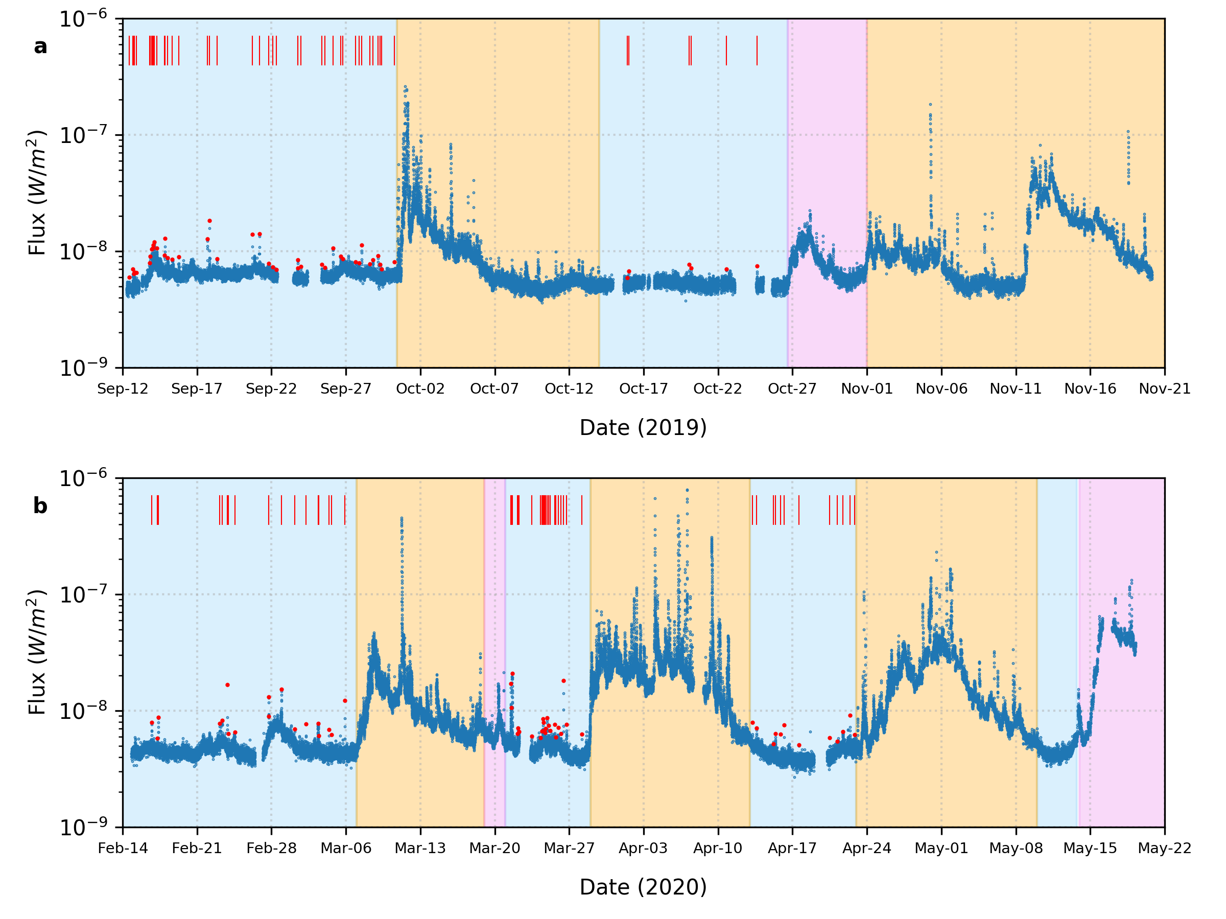
Figure 1: Panels a and b show the X-ray flux in the 1 – 15 keV energy range with a time cadence of 120 s, as measured by the XSM during two observing seasons. Different background shades represent activity levels on the Sun, with orange representing periods when NOAA active regions are present; pink representing periods of enhanced activity visible in both the XSM light curve as well as EUV/X-ray images but not classified as AR; and blue representing periods selected for the present study when no major activity was observed on the Sun. The microflares detected during the quiet periods are marked with red points, representing their peaks; and red vertical bars, representing their time.

For the selected days, we generated XSM light curves in counts for the energy band 1–5 keV with a time bin of two minutes. No solar X-ray flux was observed beyond 5 keV due to very low activity. We also generated light curves in the energy range 1.5–5 keV as microflares are expected to have a harder spectrum and thus easier to detect in the higher energy light curve. Flare like events were identified from these two light curves by using a semi-automated technique of peak identification followed by visual inspection. For each identified event, the start and end times were obtained from the light curves and only events having total counts 5$\sigma$ above the average pre-flare count rate, in either of the light curves, were selected. A total of 98 microflares were identified and the peak times these microflares are marked in Figure 1.

2.1 EUV counter parts of microflares

As the spatial location of the microflares are not available from the disk-integrated XSM observations, imaging observations in other wavelengths were used to obtain the same. For the microflares detected by the XSM, we examined concurrent EUV images of the Sun obtained with the Solar Dynamics Observatory/Atmospheric Imaging Assembly (SDO/AIA) (Lemen et al., 2012) to search for their EUV counter parts. AIA images in the shortest wavelength band at 94 $\rm{\AA}$ were used for this purpose. Synoptic AIA 94 $\rm{\AA}$ images (Level-1.5) with a cadence of two minutes available at the Joint Science Operations Center (JSOC) were obtained for the duration around each microflare. Images were examined to identify any transient events during the period of each XSM flare, and they were confirmed by generating light curve for the region around the location of the event in AIA and comparing it with the XSM light curve. EUV counterparts could be identified for 74 of the 98 microflares detected by XSM.

In order to estimate the volume of flaring region for the flares with identified EUV counterparts, we generated maps of Fe XVIII emission that trace the plasma having temperature in the range of 3-6 MK, following the approach given by Del Zanna (2013). Fe XVIII maps of a 5’ $\times$ 5’ region surrounding the microflare location were generated using the AIA images at $94\rm{\AA},211\rm{\AA},$ and $171\rm{\AA}$ at the peak of the flares using the equation

$$I(FeXVIII)=I(94\rm{\AA})-I(211\rm{\AA})/120-I(171\rm{\AA})/450$$ (1)

From the Fe XVIII images generated in this manner, the pixel having the highest intensity in the flaring region was identified and, those pixels having intensity more than 10% of the peak intensity were considered to be part of the flare event. The area of the flaring region was calculated from the number of pixels thus identified, and the volume ($V$) of the flaring plasma was estimated as $V=A^{3/2}$.

2.2 X-ray images and photospheric magnetograms

In order to examine the X-ray activity and photospheric magnetic field structure associated with the microflares, we utilized X-ray images from the Hinode X-ray Telescope (XRT) (Golub et al., 2007) and magnetograms from the SDO Helioseismic and Magnetic Imager (HMI) (Scherrer et al., 2012). From the available full disk images obtained with Hinode XRT and hourly synoptic magnetograms with SDO HMI, observations before and after the peak time of all microflares with EUV counter parts were selected. For XRT we chose images with the Be-thin filter as its efficiency curve in the low energy range is very similar to that of the XSM and thus these images are expected to represent the spatial distribution of X-ray emission observed by the XSM. Cutouts of the XRT images and HMI magnetograms for the flare location were generated for each case after taking into account the solar rotation. It may be noted that XRT images are not available at uniform intervals and in some cases the differences between the X-ray image time and the flare time are more than a day. It may also be noted that the photospheric magnetograms for near limb events may not be very reliable.

2.3 X-ray spectroscopy of microflares

We analyzed the XSM soft X-ray spectra of microflares to determine the flare temperature and emission measure. For each microflare, an interval around the peak that covers 50% of the flare duration was determined. Integrated spectra for the selected duration was generated using the XSM Data Analysis Software (XSMDAS). Spectral fitting was carried out using XSPEC package (Arnaud, 1996) with an isothermal plasma emission model based on CHIANTI atomic database version 9.0.1  (Dere et al., 1997, 2019), similar to the quiet Sun spectral analysis discussed in paper-I. The integrated spectrum of a microflare consists of emission from the flare and emission from the pre-flare quiescent Sun. Usually, spectral analysis is carried out by subtracting the pre-flare spectrum from that of the flare. However, for XSM, this may not be always appropriate as the angle subtended by the Sun with the XSM boresight varies over an orbit and thus the effective area. Therefore, instead of subtracting the quiescent emission, we obtained the quiet Sun spectral model of the respective day by fitting the observed quiet Sun spectrum for the periods excluding the flare duration with sufficient margin, as shown in Figure 2 of paper-I. It may be noted that the overall quiet Sun spectrum did not change significantly over a day. We then used a two-component model for fitting the microflare spectra, where one component is fixed to the quiet Sun spectral model and the other one belongs to the flare. For the second component corresponding to the flare emission, only the temperature and emission measure were left as free parameters in fitting while the abundances were frozen to the quiet Sun values as it is not possible to constrain elemental abundances due to low statistics of the microflare spectra. We note that the statistical uncertainties on the quiet Sun spectral model parameters are much smaller. We have verified that they have minimal impact on the estimated microflare parameters and their uncertainties, obtained by fixing the quiet Sun component at its best fit values.

3 Results and Discussion

The XSM light curves presented in Figure 1 shows several flaring events throughout the observation. During the 76 days identified when solar active regions were absent, we detected 98 microflares from XSM observations having effective exposure of 53.3 days, resulting in an average number of events to be $\sim 1.84~{}\rm{{day}^{-1}}$. Mean event rates vary from $\sim 0.75~{}\rm{{day}^{-1}}$ to $\sim 3.4~{}\rm{{day}^{-1}}$ for individual epochs of quiet Sun observations. These events are designated with IDs corresponding to the peak time, following the standard convention (Leibacher et al., 2010) and are listed in the Supplemetary Information. While a small number of such X-ray microflares occurring outside ARs have been reported earlier with Yokoh (4 microflares, Krucker et al., 1997), SphinX (16 microflares, Sylwester et al., 2019), as well as recently with NuSTAR (3 microflares, Kuhar et al., 2018), this is the first observation in X-ray wavelengths of such a large number of microflares occurring outside active regions, with the observations spanning a few months. This demonstrates that microflares are not confined only to the active regions and supports the hypothesis on presence of small scale impulsive events everywhere on the solar corona.

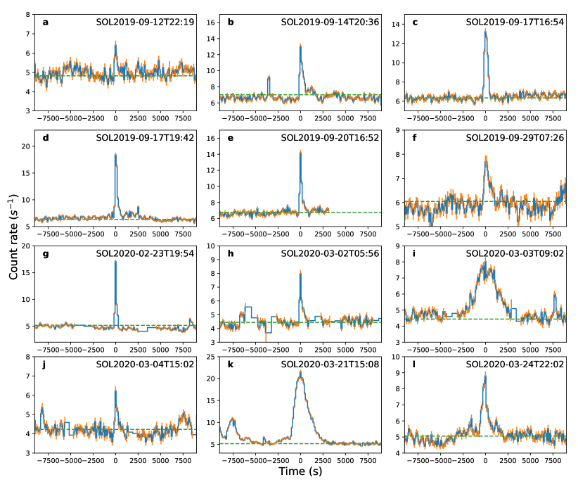
Figure 2: X-ray light curves of a representative set of microflares observed by the XSM in the energy range of 1–5 keV. Flare IDs are shown in the respective panels. Error bars correspond to one sigma uncertainties. Green dashed lines show the mean count rate for the duration considered for non-flaring quiescent emission.

X-ray light curves for a representative set of these microflares are plotted in Figure 2. Most of these microflares display a normal flare like behavior with a fast rise and slow decay, suggesting an impulsive energy release. However, there are a few microflares that do not follow this behavior possibly due to the blending of multiple microflares or due to these having an intrinsically different origin.

3.1 Microflare location

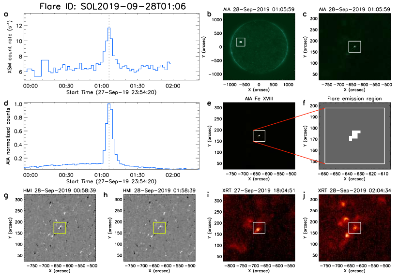
Figure 3: Identification of the location of one of the XSM microflares with the 1–5 keV light curve shown in panel a. Flare location is marked on the SDO AIA 94$~{}\rm{\AA}$ full disk image in b and a 5’ $\times$ 5’ cutout is shown in c. Panel d shows AIA 94$~{}\rm{\AA}$ light curve for the flaring pixels as shown in panel f. FeXVIII image of the flare location is shown in panel e and the map of pixels of the flaring plasma based on FeXVIII emission is given in f. Available synoptic HMI magnetograms and XRT Be-thin images nearest to the flare peak time are shown in panels g-j. The complete figure set (for all 98 microflares) is available in the online journal.

We identified the location on the solar disk for 74 of the XSM observed microflares using AIA 94 $\rm{\AA}$ images during the flare duration. Association of the X-ray events with the EUV counterpart was confirmed by comparison of the light curves. Figure 3 shows an example of the EUV counterpart identification for one microflare where the light curve for XSM is plotted in  3a and the AIA light curve for the identified region (marked in images in  3b and  3c) is shown in  3d. Similar figures for all microflares are available in the Supplementary Information. From the Fe XVIII images obtained from three AIA bands, we find that the flaring region is often very small, limited to few pixels in the images. However, there are also some cases where complex structures are resolved in the images. For uniformity, the emission volume is estimated based on number of identified pixels for all microflares.

Further, for the microflares with identified location, we examined the photospheric magnetic fields and X-ray activity before and after the microflare using synoptic data from HMI and XRT as shown in Figure  3g-  3j for one event. We find that, wherever reliable magnetograms were available, the microflares were associated with magnetic bipolar regions having weaker field strengths compared to active regions. Distinct association of microflares with bipolar regions provide an indication for magnetic reconnection in coronal loops, as in standard flare model, but at much smaller scales. We also find that most of these microflares are associated with X-ray Bright Points (XBPs, Golub et al., 1974) seen in XRT images. However, there are some microflares for which XBPs are observed before the event but not after (see flare id SOL2019-09-17T16:54 in supplementary figure) and vice-versa (e.g. flare id SOL2019-09-13T23:06). These observations can play a vital role in understanding the formation and evolution of the XBPs(Priest et al., 1994; Madjarska, 2019). More interestingly, we also find a few flares which do not appear to be associated with any XBP (e.g. flare id SOL2020-04-20T12:11); however, it is difficult to draw any specific conclusion given the large gap and non-uniform sampling between successive X-ray images.

3.2 Temperature and Emission Measure

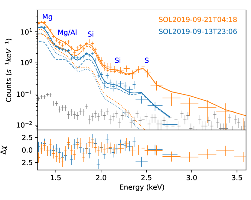
Figure 4: The XSM soft X-ray spectra for two representative microflares are shown with the fitted model. The best fit models for microflares, shown with solid lines, consists of two components: one corresponding to the background quiet Sun emission (dotted lines) and the other corresponding to the emission from the flaring plasma (dashed lines). Residuals are shown in the bottom panel. The gray color points represent the non-solar X-ray background spectrum.

By modeling the soft X-ray spectra of the microflares observed with the XSM, we obtain their temperature and emission measure (EM). Figure 4 shows the XSM spectra for two representative microflares along with the best fit models. It may be noted that the energy range for fitting is restricted typically up to 3-4 keV, where the solar spectrum dominates over the non-solar background. As seen in the figure, the spectra are well fitted with the two component model. Similar fits were obtained for other events as well. We could obtain measurements of temperature and EM with robust uncertainties for 86 of the 98 microflares, while the parameters could not be constrained for the remaining due to low statistics and hence no measurements are reported for them. Estimated spectral parameters along with other details for all the microflares are tabulated in the appendix.

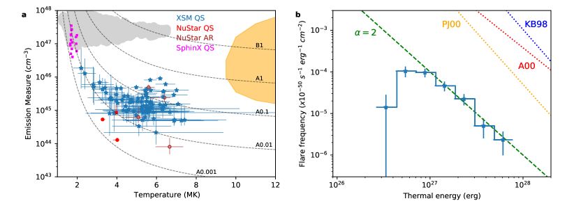
Figure 5: Panel a shows temperature and EM for 86 of the 98 quiet Sun (QS) microflares observed by the XSM with blue star symbols. The error bars represent 1$\sigma$ uncertainties. Magneta squares and red filled circles correspond to QS microflares observed by SphinX (Sylwester et al., 2019) and NuSTAR (Kuhar et al., 2018), respectively. Parameter space of active region (AR) events observed by RHESSI (Hannah et al., 2008) and SphinX (Gryciuk et al., 2017) are shown with orange and gray shades, respectively. The brown open circles represent the four AR microflares reported by NuSTAR (Wright et al., 2017; Glesener et al., 2017; Hannah et al., 2019; Cooper et al., 2020). Dashed lines represent the isoflux curves corresponding to GOES/XRS $1-8~{}\rm{\AA}$ X-ray flux levels from A0.001 ($10^{-11}~{}\rm{Wm^{-2}}$) to B1 ($10^{-7}~{}\rm{Wm^{-2}}$). Panel b shows the frequency distribution of thermal energies of 63 microflares for which the measurements are available. The green dashed line corresponds to a power law index ($\alpha$) of two shown for comparison. The dotted lines correspond to power laws reported from quiet Sun EUV observations by Krucker & Benz (1998)[KB98], Aschwanden et al. (2000b) [A00], and Parnell & Jupp (2000) [PJ00] as shown in Figure 10 of Aschwanden et al. (2000b).

Figure 5a shows EM vs temperature of the XSM microflares along with the reported measurements for microflares observed by other instruments. Isoflux curves corresponding to 1–8 $\rm{\AA}$ flux are shown with dashed lines in the figure and it can be seen from the figure that XSM detects microflares above peak a flux of $\sim 10^{-10}~{}\rm{Wm^{-2}}$. From the figure, it can be seen that the quiet Sun microflares observed by the XSM have lower temperature, EM, and thus flux compared to the sample of active region microflares observed with RHESSI (Hannah et al., 2008). However, the XSM microflare parameters are similar to those observed by NuSTAR, even though four of the seven NuSTAR microflares have been observed within active regions. This suggests that the basic physical processes in the non-AR microflares observed by XSM are similar to those in the active region microflares and may differ only in terms of the scale.

Two of the quiet Sun microflares observed by NuSTAR (Kuhar et al., 2018) are weaker than all the events observed by the XSM, which is expected given the sensitivity of NuSTAR. We also note that the 16 microflares observed by SphinX show a systematically lower temperature and higher EM compared to the microflares observed by XSM as well as NuSTAR. One possible reason for this observation may be the difference in analysis procedure followed for SphinX data where the flare spectra were fitted with a single temperature model without subtracting or separately modelling the pre-flare emission (Sylwester et al., 2019). While the microflares observed by SphinX and XSM occupy slightly different regions in the temperature-EM parameter space, the fact that they fall along the same isoflux line shows that they should be of similar nature.

3.3 Microflare thermal energy distribution

Using the temperature ($T$) and emission measure ($EM$) obtained from X-ray spectroscopy and the plasma volume ($V$) obtained from the AIA images, we estimated the thermal energy associated with each microflare (Hannah et al., 2008) as

$$E_{th}\sim 3~{}k_{\rm{B}}T~{}\sqrt{EM\times V}$$ (2)

where $k_{\rm{B}}$ is the Boltzmann constant. This assumes a filling factor of unity, which is an upper limit. Further, as the volume is estimated from lower energy emission, it also can be considered as an upper limit to the actual volume and thus the energy estimates represent upper limits. Of the total 98 microflares, thermal energy could be estimated for 63 flares for which measurements of all three parameters are available (see appendix). Errors on thermal energy were computed by propagating the errors on temperature and emission measure. We find that the thermal energies of XSM microflares ranges from $3\times 10^{26}-7\times 10^{27}\rm{erg}$. A histogram of thermal energies of the microflares was then generated and is normalized with the total exposure time and area, which is shown in Figure 5b. Error bars on the histogram are computed considering counting statistics. A power law of index two is overplotted in the figure with dashed line for comparison and it can be seen that frequency distribution agrees with the power law. The Departure from power law seen at the lower energy end is expected from the fact that fainter events are less likely to be detected against the background quiet Sun emission. A similar trend has been seen in the distribution of active region flares from previous studies (Hannah et al., 2011).

Even though the present observations provide the largest sample of microflares in the quiet Sun, the total number is not sufficient for quantitative estimation of the power law index. However, Figure 5b shows with certainty that the observed histogram is significantly different from the power law derived from previous quiet Sun EUV nanoflare observations (Krucker & Benz, 1998; Aschwanden et al., 2000b; Parnell & Jupp, 2000) extrapolated to higher energies. It should be noted that two of the flare frequency histograms in EUV are obtained during solar minimum in 1998-99 and thus the difference may not be due to solar activity. This suggests that the difference may be either due to a change in power law index over the typical nanoflare to microflare energies or the EUV and X-ray events are from two different populations. In any case, our observations, being the first statistical survey of X-ray microflares outside active regions, are expected to provide crucial inputs to understand the role of small scale impulsive events in coronal heating.

Another point to note is that the present work, like most others, considered only the energy associated with the thermal emission, The total energy may include other components such as non-thermal accelerated particles and waves and it is important to understand the energy partition into these (Benz, 2017). With sensitive X-ray spectroscopic observations, it has been possible to disentangle thermal and non-thermal components in A class microflare (Glesener et al., 2020). Broad-band X-ray observations of small scale events using the XSM along with hard X-ray instruments such as Solar Orbiter STIX (Krucker et al., 2020) and NuSTAR will help in improving the understanding of thermal and non-thermal energy associated with such events, so that better estimates of total energy can be obtained.

4 Summary

We presented the largest sample of X-ray microflares in the quiet Sun using disk-integrated observations with the Chandrayaan-2 XSM. From XSM observations during extended periods without active regions on the solar disk, 98 sub-A class microflares were detected. We find that most of the microflares are impulsive in nature and in all cases where the microflare location is identified, they are associated with magnetic bipolar regions. Using the results of spectroscopic analysis of the XSM data and analysis of EUV images, we estimated that the thermal energies of these microflares range from $\sim 3\times 10^{26}$ – $6\times 10^{27}$ erg and the flare frequency distribution follows a power law. The present observations provide a stringent limit on the average number of microflares having flux above $\sim 10^{-10}~{}\rm{Wm^{-2}}$ (thermal energies above $\sim 4-7\times 10^{26}$erg) ocurring in the quiet Sun. During the period of observed extremely quiet solar corona, having no active region on the disk, the flare rate is found to be $\sim 1.84~{}\rm{{day}^{-1}}$, while the mean values for each epoch vary from $\sim 0.75~{}\rm{{day}^{-1}}$ to $\sim 3.4~{}\rm{{day}^{-1}}$. While the statistics may not be sufficient to constrain the index of the power law very well, these observations provide strong support to the hypothesis of occurrence of small scale impulsive heating events everywhere on the solar disk, which could contribute to the heating of the corona.

Appendix A Microflare Parameters

Table 1: Micoflares observed by XSM in the quiet Sun period (blue shaded region in Figure 1).
^aFlare ID correspond to the time at the peak of the flare in the format SOL$yyyy$-$mm$-$dd$T$hh$:$mm$.
^bPeak count rate and peak flux include the pre-flare emission rate/flux.
^cTemperature, volume EM, and flare flux are estimated for the flaring plasma alone. Pre-flare emission is modelled as a separate component as discussed in the text.
^dNumber of pixels in AIA FeXVIII image at the peak of the flare providing the area ($A$) of the flaring region. Each pixel correspond to area of 2.4” x 2.4”. Volume ($V$) of the flaring plasma is estimated as $V=A^{3/2}$.
^eThermal energy estimated for flares with temperature, EM, and volume measurement available.
^∗Flux values are shown in units of $10^{-8}~{}\mathrm{Wm^{-2}}$ corresponding to A level of GOES/XRS X-ray intensity scale.

Sl No	Flare IDa	Peak rateb	Peak 1-8$\mathrm{\AA}$ fluxb∗	Temperaturec	Volume EMc	Flare 1-8$\mathrm{\AA}$ fluxc∗	No. of pixelsd	$\mathrm{E_{thermal}}^{e}$
		($\mathrm{s^{-1}}$)	(x$10^{-8}~{}\mathrm{Wm^{-2}}$)	(MK)	(x$10^{46}~{}\mathrm{{cm}^{-3}}$)	(x$10^{-8}~{}\mathrm{Wm^{-2}}$)	AIA FeXVIII	(erg)
1	SOL2019-09-12T11:01	6.7	0.09	$3.6\begin{subarray}{c}+2.4\\ -1.2\end{subarray}$	$0.08\begin{subarray}{c}+0.41\\ -0.06\end{subarray}$	0.007	32	$1.3\begin{subarray}{c}+3.4\\ -0.7\end{subarray}\times 10^{27}$
2	SOL2019-09-12T16:07	8.4	0.13	$5.8\begin{subarray}{c}+1.3\\ -0.8\end{subarray}$	$0.09\begin{subarray}{c}+0.04\\ -0.03\end{subarray}$	0.039	-	-
3	SOL2019-09-12T18:33	7.9	0.11	$7.3\begin{subarray}{c}+1.9\\ -2.9\end{subarray}$	$0.05\begin{subarray}{c}+0.11\\ -0.02\end{subarray}$	0.037	29	$1.9\begin{subarray}{c}+2.1\\ -0.8\end{subarray}\times 10^{27}$
4	SOL2019-09-12T22:19	7.6	0.13	-	-	-	10	-
5	SOL2019-09-13T19:16	9.3	0.14	$3.4\begin{subarray}{c}+0.6\\ -0.5\end{subarray}$	$0.47\begin{subarray}{c}+0.41\\ -0.22\end{subarray}$	0.029	11	$1.3\begin{subarray}{c}+0.6\\ -0.4\end{subarray}\times 10^{27}$
6	SOL2019-09-13T20:38	10.6	0.18	$5.0\begin{subarray}{c}+0.7\\ -0.6\end{subarray}$	$0.18\begin{subarray}{c}+0.08\\ -0.05\end{subarray}$	0.052	10	$1.1\begin{subarray}{c}+0.3\\ -0.2\end{subarray}\times 10^{27}$
7	SOL2019-09-13T23:06	12.0	0.21	$4.0\begin{subarray}{c}+0.3\\ -0.3\end{subarray}$	$0.46\begin{subarray}{c}+0.12\\ -0.10\end{subarray}$	0.057	39	$4.0\begin{subarray}{c}+0.6\\ -0.5\end{subarray}\times 10^{27}$
8	SOL2019-09-14T00:42	12.4	0.20	$5.1\begin{subarray}{c}+0.7\\ -0.6\end{subarray}$	$0.23\begin{subarray}{c}+0.10\\ -0.06\end{subarray}$	0.067	-	-
9	SOL2019-09-14T01:48	13.3	0.24	$5.7\begin{subarray}{c}+0.5\\ -0.5\end{subarray}$	$0.17\begin{subarray}{c}+0.05\\ -0.03\end{subarray}$	0.069	22	$2.2\begin{subarray}{c}+0.4\\ -0.3\end{subarray}\times 10^{27}$
10	SOL2019-09-14T03:24	14.2	0.23	$4.2\begin{subarray}{c}+0.3\\ -0.2\end{subarray}$	$0.46\begin{subarray}{c}+0.09\\ -0.08\end{subarray}$	0.071	-	-
11	SOL2019-09-14T07:04	12.3	0.20	$4.5\begin{subarray}{c}+0.4\\ -0.4\end{subarray}$	$0.27\begin{subarray}{c}+0.08\\ -0.06\end{subarray}$	0.055	33	$3.1\begin{subarray}{c}+0.5\\ -0.4\end{subarray}\times 10^{27}$
12	SOL2019-09-14T19:38	10.4	0.19	$6.9\begin{subarray}{c}+1.3\\ -1.1\end{subarray}$	$0.05\begin{subarray}{c}+0.00\\ -0.01\end{subarray}$	0.034	5	$4.9\begin{subarray}{c}+1.0\\ -1.0\end{subarray}\times 10^{26}$
13	SOL2019-09-14T20:36	14.6	0.32	$5.5\begin{subarray}{c}+0.6\\ -0.6\end{subarray}$	$0.25\begin{subarray}{c}+0.07\\ -0.05\end{subarray}$	0.095	6	$1.0\begin{subarray}{c}+0.2\\ -0.1\end{subarray}\times 10^{27}$
14	SOL2019-09-15T00:42	9.7	0.30	$3.6\begin{subarray}{c}+0.7\\ -0.5\end{subarray}$	$0.22\begin{subarray}{c}+0.18\\ -0.10\end{subarray}$	0.019	-	-
15	SOL2019-09-15T08:16	9.9	0.16	$4.0\begin{subarray}{c}+0.5\\ -0.4\end{subarray}$	$0.30\begin{subarray}{c}+0.15\\ -0.10\end{subarray}$	0.036	-	-
16	SOL2019-09-17T16:54	14.9	0.30	$5.7\begin{subarray}{c}+0.5\\ -0.5\end{subarray}$	$0.40\begin{subarray}{c}+0.09\\ -0.06\end{subarray}$	0.166	5	$1.1\begin{subarray}{c}+0.2\\ -0.1\end{subarray}\times 10^{27}$
17	SOL2019-09-17T19:42	20.3	0.59	$7.0\begin{subarray}{c}+0.6\\ -0.7\end{subarray}$	$0.40\begin{subarray}{c}+0.08\\ -0.05\end{subarray}$	0.276	-	-
18	SOL2019-09-18T08:36	10.1	0.17	$5.5\begin{subarray}{c}+1.0\\ -0.8\end{subarray}$	$0.14\begin{subarray}{c}+0.07\\ -0.04\end{subarray}$	0.051	-	-
19	SOL2019-09-20T16:52	15.8	0.36	$6.3\begin{subarray}{c}+0.5\\ -0.5\end{subarray}$	$0.25\begin{subarray}{c}+0.06\\ -0.04\end{subarray}$	0.139	35	$4.3\begin{subarray}{c}+0.6\\ -0.5\end{subarray}\times 10^{27}$
20	SOL2019-09-21T04:18	16.1	0.38	$6.4\begin{subarray}{c}+0.5\\ -0.5\end{subarray}$	$0.37\begin{subarray}{c}+0.07\\ -0.05\end{subarray}$	0.203	-	-
21	SOL2019-09-21T19:18	9.4	0.11	$2.2\begin{subarray}{c}+0.6\\ -0.4\end{subarray}$	$1.86\begin{subarray}{c}+5.86\\ -1.40\end{subarray}$	0.008	9	$1.5\begin{subarray}{c}+2.4\\ -0.6\end{subarray}\times 10^{27}$
22	SOL2019-09-22T01:58	8.8	0.11	-	-	-	17	-
23	SOL2019-09-22T07:32	8.4	0.11	-	-	-	7	-
24	SOL2019-09-23T18:04	8.4	0.13	$4.0\begin{subarray}{c}+1.5\\ -1.1\end{subarray}$	$0.20\begin{subarray}{c}+0.48\\ -0.12\end{subarray}$	0.025	-	-
25	SOL2019-09-23T18:32	9.9	0.15	$6.3\begin{subarray}{c}+3.9\\ -1.4\end{subarray}$	$0.11\begin{subarray}{c}+0.09\\ -0.05\end{subarray}$	0.060	-	-
26	SOL2019-09-23T23:04	8.4	0.13	$6.9\begin{subarray}{c}+1.5\\ -2.4\end{subarray}$	$0.05\begin{subarray}{c}+0.08\\ -0.01\end{subarray}$	0.032	6	$5.5\begin{subarray}{c}+4.8\\ -2.1\end{subarray}\times 10^{26}$
27	SOL2019-09-25T08:50	8.7	0.11	$5.0\begin{subarray}{c}+1.9\\ -1.3\end{subarray}$	$0.07\begin{subarray}{c}+0.11\\ -0.04\end{subarray}$	0.020	6	$4.8\begin{subarray}{c}+4.1\\ -1.8\end{subarray}\times 10^{26}$
28	SOL2019-09-26T03:32	12.3	0.21	$7.1\begin{subarray}{c}+0.6\\ -0.5\end{subarray}$	$0.15\begin{subarray}{c}+0.02\\ -0.02\end{subarray}$	0.109	12	$1.7\begin{subarray}{c}+0.2\\ -0.2\end{subarray}\times 10^{27}$
29	SOL2019-09-26T15:50	10.8	0.17	$4.4\begin{subarray}{c}+0.5\\ -0.4\end{subarray}$	$0.26\begin{subarray}{c}+0.09\\ -0.07\end{subarray}$	0.047	-	-
30	SOL2019-09-26T18:34	10.3	0.12	$3.1\begin{subarray}{c}+0.4\\ -0.4\end{subarray}$	$0.69\begin{subarray}{c}+0.50\\ -0.28\end{subarray}$	0.029	-	-
31	SOL2019-09-27T15:32	9.5	0.14	$4.5\begin{subarray}{c}+1.5\\ -1.2\end{subarray}$	$0.09\begin{subarray}{c}+0.17\\ -0.05\end{subarray}$	0.018	-	-
32	SOL2019-09-27T21:00	9.5	0.10	$5.1\begin{subarray}{c}+1.6\\ -1.3\end{subarray}$	$0.03\begin{subarray}{c}+0.00\\ -0.02\end{subarray}$	0.010	-	-
33	SOL2019-09-28T01:06	13.2	0.24	$5.5\begin{subarray}{c}+0.5\\ -0.5\end{subarray}$	$0.30\begin{subarray}{c}+0.08\\ -0.06\end{subarray}$	0.109	9	$1.5\begin{subarray}{c}+0.2\\ -0.2\end{subarray}\times 10^{27}$
34	SOL2019-09-28T14:16	9.2	0.11	$2.4\begin{subarray}{c}+0.6\\ -0.4\end{subarray}$	$1.28\begin{subarray}{c}+2.32\\ -0.85\end{subarray}$	0.011	17	$2.1\begin{subarray}{c}+2.0\\ -0.8\end{subarray}\times 10^{27}$
35	SOL2019-09-28T19:42	9.9	0.13	$4.8\begin{subarray}{c}+0.7\\ -0.6\end{subarray}$	$0.18\begin{subarray}{c}+0.08\\ -0.06\end{subarray}$	0.044	16	$1.5\begin{subarray}{c}+0.4\\ -0.3\end{subarray}\times 10^{27}$
36	SOL2019-09-29T04:04	10.4	0.19	$5.6\begin{subarray}{c}+2.3\\ -1.7\end{subarray}$	$0.09\begin{subarray}{c}+0.17\\ -0.05\end{subarray}$	0.036	8	$7.6\begin{subarray}{c}+7.8\\ -3.0\end{subarray}\times 10^{26}$
37	SOL2019-09-29T07:26	9.1	0.13	$7.4\begin{subarray}{c}+2.1\\ -2.7\end{subarray}$	$0.05\begin{subarray}{c}+0.09\\ -0.02\end{subarray}$	0.040	-	-
38	SOL2019-09-29T09:54	8.2	0.13	-	-	-	-	-
39	SOL2019-09-30T06:22	9.4	0.17	$4.9\begin{subarray}{c}+2.8\\ -1.4\end{subarray}$	$0.09\begin{subarray}{c}+0.18\\ -0.06\end{subarray}$	0.024	8	$6.7\begin{subarray}{c}+7.6\\ -2.9\end{subarray}\times 10^{26}$
40	SOL2019-10-15T21:25	7.2	0.08	-	-	-	13	-
41	SOL2019-10-15T23:47	8.0	0.11	-	-	-	8	-
42	SOL2019-10-20T01:34	8.8	0.13	$3.7\begin{subarray}{c}+1.2\\ -1.2\end{subarray}$	$0.24\begin{subarray}{c}+0.93\\ -0.14\end{subarray}$	0.022	6	$6.5\begin{subarray}{c}+12.8\\ -2.8\end{subarray}\times 10^{26}$
43	SOL2019-10-20T04:38	8.1	0.17	$4.3\begin{subarray}{c}+1.3\\ -1.0\end{subarray}$	$0.10\begin{subarray}{c}+0.15\\ -0.05\end{subarray}$	0.017	10	$7.3\begin{subarray}{c}+5.8\\ -2.6\end{subarray}\times 10^{26}$
44	SOL2019-10-22T13:18	8.3	0.12	$5.7\begin{subarray}{c}+1.1\\ -0.9\end{subarray}$	$0.12\begin{subarray}{c}+0.06\\ -0.04\end{subarray}$	0.051	8	$9.0\begin{subarray}{c}+2.8\\ -1.9\end{subarray}\times 10^{26}$
45	SOL2019-10-24T14:32	8.4	0.20	-	-	-	6	-
46	SOL2020-02-16T18:00	9.2	0.18	$6.5\begin{subarray}{c}+0.9\\ -0.7\end{subarray}$	$0.15\begin{subarray}{c}+0.04\\ -0.03\end{subarray}$	0.084	7	$1.0\begin{subarray}{c}+0.2\\ -0.1\end{subarray}\times 10^{27}$
47	SOL2020-02-17T06:30	6.9	0.10	$4.0\begin{subarray}{c}+1.2\\ -0.9\end{subarray}$	$0.17\begin{subarray}{c}+0.23\\ -0.09\end{subarray}$	0.022	29	$1.9\begin{subarray}{c}+1.5\\ -0.7\end{subarray}\times 10^{27}$
48	SOL2020-02-17T08:34	10.2	0.20	$5.5\begin{subarray}{c}+0.5\\ -0.5\end{subarray}$	$0.33\begin{subarray}{c}+0.08\\ -0.06\end{subarray}$	0.123	4	$8.4\begin{subarray}{c}+1.3\\ -1.1\end{subarray}\times 10^{26}$
49	SOL2020-02-23T02:38	9.1	0.16	$5.6\begin{subarray}{c}+1.2\\ -0.9\end{subarray}$	$0.11\begin{subarray}{c}+0.06\\ -0.04\end{subarray}$	0.044	8	$8.4\begin{subarray}{c}+3.0\\ -2.0\end{subarray}\times 10^{26}$
50	SOL2020-02-23T08:38	9.4	0.17	$6.2\begin{subarray}{c}+0.7\\ -0.7\end{subarray}$	$0.15\begin{subarray}{c}+0.04\\ -0.03\end{subarray}$	0.076	25	$2.5\begin{subarray}{c}+0.5\\ -0.4\end{subarray}\times 10^{27}$
51	SOL2020-02-23T19:54	18.5	0.54	$6.9\begin{subarray}{c}+0.7\\ -0.7\end{subarray}$	$0.29\begin{subarray}{c}+0.06\\ -0.04\end{subarray}$	0.191	6	$1.3\begin{subarray}{c}+0.2\\ -0.2\end{subarray}\times 10^{27}$
52	SOL2020-02-23T22:12	7.4	0.10	-	-	-	8	-
53	SOL2020-02-24T13:54	7.7	0.11	-	-	-	8	-
54	SOL2020-02-27T17:14	10.2	0.21	$5.3\begin{subarray}{c}+0.6\\ -0.6\end{subarray}$	$0.24\begin{subarray}{c}+0.09\\ -0.06\end{subarray}$	0.081	-	-
55	SOL2020-02-27T17:58	15.1	0.32	$6.3\begin{subarray}{c}+0.3\\ -0.3\end{subarray}$	$0.37\begin{subarray}{c}+0.04\\ -0.03\end{subarray}$	0.200	17	$3.0\begin{subarray}{c}+0.2\\ -0.2\end{subarray}\times 10^{27}$
56	SOL2020-02-28T22:24	17.1	0.39	$5.5\begin{subarray}{c}+0.4\\ -0.3\end{subarray}$	$0.43\begin{subarray}{c}+0.07\\ -0.07\end{subarray}$	0.163	7	$1.5\begin{subarray}{c}+0.2\\ -0.1\end{subarray}\times 10^{27}$
57	SOL2020-03-01T04:30	8.1	0.11	$6.7\begin{subarray}{c}+0.9\\ -0.8\end{subarray}$	$0.09\begin{subarray}{c}+0.03\\ -0.02\end{subarray}$	0.055	37	$2.8\begin{subarray}{c}+0.6\\ -0.5\end{subarray}\times 10^{27}$
58	SOL2020-03-02T05:56	9.1	0.16	$5.8\begin{subarray}{c}+1.0\\ -0.9\end{subarray}$	$0.15\begin{subarray}{c}+0.07\\ -0.04\end{subarray}$	0.066	5	$7.1\begin{subarray}{c}+2.1\\ -1.5\end{subarray}\times 10^{26}$
59	SOL2020-03-03T09:02	9.2	0.17	$5.5\begin{subarray}{c}+0.3\\ -0.3\end{subarray}$	$0.19\begin{subarray}{c}+0.02\\ -0.02\end{subarray}$	0.071	-	-
60	SOL2020-03-03T11:10	7.2	0.11	$2.8\begin{subarray}{c}+1.0\\ -0.6\end{subarray}$	$0.51\begin{subarray}{c}+1.40\\ -0.36\end{subarray}$	0.013	29	$2.4\begin{subarray}{c}+3.4\\ -1.0\end{subarray}\times 10^{27}$
61	SOL2020-03-04T09:56	7.8	0.15	$5.7\begin{subarray}{c}+1.8\\ -1.3\end{subarray}$	$0.11\begin{subarray}{c}+0.10\\ -0.04\end{subarray}$	0.044	4	$5.0\begin{subarray}{c}+2.8\\ -1.5\end{subarray}\times 10^{26}$
62	SOL2020-03-04T15:02	7.1	0.13	$5.5\begin{subarray}{c}+7.2\\ -1.4\end{subarray}$	$0.09\begin{subarray}{c}+0.11\\ -0.05\end{subarray}$	0.032	8	$7.2\begin{subarray}{c}+10.5\\ -2.9\end{subarray}\times 10^{26}$
63	SOL2020-03-05T21:40	14.0	0.35	$5.4\begin{subarray}{c}+0.4\\ -0.4\end{subarray}$	$0.39\begin{subarray}{c}+0.07\\ -0.06\end{subarray}$	0.142	6	$1.2\begin{subarray}{c}+0.1\\ -0.1\end{subarray}\times 10^{27}$
64	SOL2020-03-21T12:20	19.2	0.47	$5.7\begin{subarray}{c}+0.3\\ -0.3\end{subarray}$	$0.82\begin{subarray}{c}+0.11\\ -0.09\end{subarray}$	0.336	38	$7.4\begin{subarray}{c}+0.7\\ -0.6\end{subarray}\times 10^{27}$
65	SOL2020-03-21T13:02	12.5	0.23	$5.0\begin{subarray}{c}+0.3\\ -0.3\end{subarray}$	$0.49\begin{subarray}{c}+0.08\\ -0.07\end{subarray}$	0.137	40	$5.2\begin{subarray}{c}+0.5\\ -0.5\end{subarray}\times 10^{27}$
66	SOL2020-03-21T15:08	23.6	0.61	$6.2\begin{subarray}{c}+0.1\\ -0.2\end{subarray}$	$0.90\begin{subarray}{c}+0.06\\ -0.04\end{subarray}$	0.466	31	$7.3\begin{subarray}{c}+0.3\\ -0.3\end{subarray}\times 10^{27}$
67	SOL2020-03-22T03:34	7.5	0.10	$4.6\begin{subarray}{c}+1.9\\ -1.7\end{subarray}$	$0.11\begin{subarray}{c}+0.41\\ -0.06\end{subarray}$	0.022	5	$4.7\begin{subarray}{c}+9.4\\ -2.2\end{subarray}\times 10^{26}$
68	SOL2020-03-22T04:18	8.6	0.17	$5.7\begin{subarray}{c}+1.0\\ -0.8\end{subarray}$	$0.18\begin{subarray}{c}+0.08\\ -0.05\end{subarray}$	0.076	28	$2.8\begin{subarray}{c}+0.8\\ -0.5\end{subarray}\times 10^{27}$
69	SOL2020-03-22T06:08	8.0	0.11	$5.5\begin{subarray}{c}+1.1\\ -1.0\end{subarray}$	$0.12\begin{subarray}{c}+0.07\\ -0.04\end{subarray}$	0.043	31	$2.3\begin{subarray}{c}+0.9\\ -0.6\end{subarray}\times 10^{27}$
70	SOL2020-03-23T10:57	7.2	0.11	$4.3\begin{subarray}{c}+0.9\\ -0.7\end{subarray}$	$0.20\begin{subarray}{c}+0.18\\ -0.09\end{subarray}$	0.033	6	$7.0\begin{subarray}{c}+3.5\\ -1.9\end{subarray}\times 10^{26}$
71	SOL2020-03-24T07:32	6.9	0.08	$6.0\begin{subarray}{c}+3.4\\ -2.6\end{subarray}$	$0.02\begin{subarray}{c}+0.09\\ -0.01\end{subarray}$	0.010	-	-
72	SOL2020-03-24T11:10	7.9	0.11	$5.5\begin{subarray}{c}+1.6\\ -1.3\end{subarray}$	$0.10\begin{subarray}{c}+0.10\\ -0.04\end{subarray}$	0.035	-	-
73	SOL2020-03-24T12:56	9.8	0.16	$4.7\begin{subarray}{c}+0.6\\ -0.6\end{subarray}$	$0.21\begin{subarray}{c}+0.11\\ -0.06\end{subarray}$	0.049	7	$8.8\begin{subarray}{c}+2.5\\ -1.7\end{subarray}\times 10^{26}$
74	SOL2020-03-24T14:24	9.2	0.14	$5.3\begin{subarray}{c}+1.1\\ -0.9\end{subarray}$	$0.13\begin{subarray}{c}+0.08\\ -0.04\end{subarray}$	0.042	5	$5.9\begin{subarray}{c}+2.2\\ -1.4\end{subarray}\times 10^{26}$
75	SOL2020-03-24T15:36	7.8	0.13	$2.8\begin{subarray}{c}+1.0\\ -0.6\end{subarray}$	$0.59\begin{subarray}{c}+1.46\\ -0.43\end{subarray}$	0.014	-	-
76	SOL2020-03-24T17:44	7.7	0.12	$3.7\begin{subarray}{c}+0.9\\ -0.7\end{subarray}$	$0.21\begin{subarray}{c}+0.24\\ -0.10\end{subarray}$	0.020	8	$7.7\begin{subarray}{c}+4.7\\ -2.4\end{subarray}\times 10^{26}$
77	SOL2020-03-24T22:02	10.2	0.16	$6.4\begin{subarray}{c}+0.7\\ -0.6\end{subarray}$	$0.14\begin{subarray}{c}+0.03\\ -0.02\end{subarray}$	0.075	20	$2.1\begin{subarray}{c}+0.3\\ -0.3\end{subarray}\times 10^{27}$
78	SOL2020-03-25T01:56	8.6	0.14	$4.3\begin{subarray}{c}+0.9\\ -0.7\end{subarray}$	$0.21\begin{subarray}{c}+0.17\\ -0.09\end{subarray}$	0.034	-	-
79	SOL2020-03-25T05:28	8.0	0.13	$5.3\begin{subarray}{c}+2.2\\ -1.5\end{subarray}$	$0.05\begin{subarray}{c}+0.09\\ -0.03\end{subarray}$	0.017	4	$3.2\begin{subarray}{c}+3.1\\ -1.3\end{subarray}\times 10^{26}$
80	SOL2020-03-25T14:50	9.0	0.16	$5.2\begin{subarray}{c}+1.2\\ -0.9\end{subarray}$	$0.10\begin{subarray}{c}+0.07\\ -0.04\end{subarray}$	0.034	9	$8.3\begin{subarray}{c}+3.4\\ -2.1\end{subarray}\times 10^{26}$
81	SOL2020-03-25T17:14	6.9	0.11	-	-	-	12	-
82	SOL2020-03-25T23:22	8.4	0.13	$3.9\begin{subarray}{c}+2.1\\ -1.2\end{subarray}$	$0.08\begin{subarray}{c}+0.28\\ -0.06\end{subarray}$	0.009	8	$5.0\begin{subarray}{c}+8.9\\ -2.4\end{subarray}\times 10^{26}$
83	SOL2020-03-26T05:00	7.2	0.12	$3.5\begin{subarray}{c}+0.9\\ -0.6\end{subarray}$	$0.34\begin{subarray}{c}+0.42\\ -0.19\end{subarray}$	0.023	25	$2.1\begin{subarray}{c}+1.4\\ -0.7\end{subarray}\times 10^{27}$
84	SOL2020-03-26T11:00	20.0	0.57	$6.5\begin{subarray}{c}+0.5\\ -0.5\end{subarray}$	$0.61\begin{subarray}{c}+0.10\\ -0.07\end{subarray}$	0.349	5	$1.6\begin{subarray}{c}+0.2\\ -0.2\end{subarray}\times 10^{27}$
85	SOL2020-03-26T17:30	8.7	0.14	$5.8\begin{subarray}{c}+0.9\\ -0.7\end{subarray}$	$0.12\begin{subarray}{c}+0.05\\ -0.03\end{subarray}$	0.050	4	$5.3\begin{subarray}{c}+1.3\\ -1.0\end{subarray}\times 10^{26}$
86	SOL2020-03-28T04:18	7.4	0.13	$5.3\begin{subarray}{c}+0.9\\ -0.7\end{subarray}$	$0.14\begin{subarray}{c}+0.07\\ -0.04\end{subarray}$	0.047	-	-
87	SOL2020-04-13T05:28	9.2	0.16	$3.3\begin{subarray}{c}+0.8\\ -0.5\end{subarray}$	$0.43\begin{subarray}{c}+0.51\\ -0.23\end{subarray}$	0.023	6	$7.7\begin{subarray}{c}+5.0\\ -2.5\end{subarray}\times 10^{26}$
88	SOL2020-04-13T14:20	8.5	0.14	-	-	-	7	-
89	SOL2020-04-15T05:20	6.2	0.08	$5.4\begin{subarray}{c}+0.8\\ -1.2\end{subarray}$	$0.06\begin{subarray}{c}+0.06\\ -0.02\end{subarray}$	0.022	24	$1.4\begin{subarray}{c}+0.7\\ -0.4\end{subarray}\times 10^{27}$
90	SOL2020-04-15T09:16	7.4	0.11	$4.6\begin{subarray}{c}+0.7\\ -0.6\end{subarray}$	$0.17\begin{subarray}{c}+0.08\\ -0.05\end{subarray}$	0.038	19	$1.7\begin{subarray}{c}+0.5\\ -0.3\end{subarray}\times 10^{27}$
91	SOL2020-04-15T20:44	7.3	0.15	$5.6\begin{subarray}{c}+1.5\\ -1.3\end{subarray}$	$0.10\begin{subarray}{c}+0.10\\ -0.04\end{subarray}$	0.039	6	$6.3\begin{subarray}{c}+3.6\\ -1.9\end{subarray}\times 10^{26}$
92	SOL2020-04-16T05:34	8.6	0.18	$6.3\begin{subarray}{c}+0.7\\ -0.6\end{subarray}$	$0.11\begin{subarray}{c}+0.03\\ -0.02\end{subarray}$	0.061	8	$9.5\begin{subarray}{c}+1.6\\ -1.3\end{subarray}\times 10^{26}$
93	SOL2020-04-17T14:02	6.2	0.08	$5.6\begin{subarray}{c}+1.7\\ -1.3\end{subarray}$	$0.09\begin{subarray}{c}+0.08\\ -0.04\end{subarray}$	0.036	10	$9.0\begin{subarray}{c}+4.9\\ -2.7\end{subarray}\times 10^{26}$
94	SOL2020-04-20T12:11	6.8	0.12	$5.3\begin{subarray}{c}+1.4\\ -1.0\end{subarray}$	$0.08\begin{subarray}{c}+0.07\\ -0.03\end{subarray}$	0.029	6	$5.6\begin{subarray}{c}+2.6\\ -1.6\end{subarray}\times 10^{26}$
95	SOL2020-04-21T05:10	6.7	0.08	-	-	-	12	-
96	SOL2020-04-21T17:26	7.9	0.12	$4.4\begin{subarray}{c}+0.7\\ -0.5\end{subarray}$	$0.13\begin{subarray}{c}+0.06\\ -0.05\end{subarray}$	0.025	-	-
97	SOL2020-04-22T09:16	10.3	0.21	$5.2\begin{subarray}{c}+0.8\\ -0.6\end{subarray}$	$0.18\begin{subarray}{c}+0.08\\ -0.05\end{subarray}$	0.058	5	$7.0\begin{subarray}{c}+1.8\\ -1.3\end{subarray}\times 10^{26}$
98	SOL2020-04-22T20:48	7.3	0.13	$5.9\begin{subarray}{c}+1.4\\ -1.1\end{subarray}$	$0.06\begin{subarray}{c}+0.00\\ -0.02\end{subarray}$	0.025	14	$9.4\begin{subarray}{c}+2.3\\ -2.4\end{subarray}\times 10^{26}$

References

- Arnaud (1996) Arnaud, K. A. 1996, in Astronomical Society of the Pacific Conference Series, Vol. 101, Astronomical Data Analysis Software and Systems V, ed. G. H. Jacoby & J. Barnes, 17
- Aschwanden et al. (2000a) Aschwanden, M. J., Nightingale, R. W., Tarbell, T. D., & Wolfson, C. J. 2000a, ApJ, 535, 1027, doi: 10.1086/308866
- Aschwanden et al. (2000b) Aschwanden, M. J., Tarbell, T. D., Nightingale, R. W., et al. 2000b, ApJ, 535, 1047, doi: 10.1086/308867
- Benz (2017) Benz, A. O. 2017, Living Reviews in Solar Physics, 14, 2, doi: 10.1007/s41116-016-0004-3
- Benz & Krucker (2002) Benz, A. O., & Krucker, S. 2002, ApJ, 568, 413, doi: 10.1086/338807
- Christe et al. (2008) Christe, S., Hannah, I. G., Krucker, S., McTiernan, J., & Lin, R. P. 2008, ApJ, 677, 1385, doi: 10.1086/529011
- Cooper et al. (2020) Cooper, K., Hannah, I. G., Grefenstette, B. W., et al. 2020, ApJ, 893, L40, doi: 10.3847/2041-8213/ab873e
- Del Zanna (2013) Del Zanna, G. 2013, A&A, 558, A73, doi: 10.1051/0004-6361/201321653
- Dere et al. (2019) Dere, K. P., Del Zanna, G., Young, P. R., Landi, E., & Sutherland, R. S. 2019, ApJS, 241, 22, doi: 10.3847/1538-4365/ab05cf
- Dere et al. (1997) Dere, K. P., Landi, E., Mason, H. E., Monsignori Fossi, B. C., & Young, P. R. 1997, A&AS, 125, 149, doi: 10.1051/aas:1997368
- Glesener et al. (2017) Glesener, L., Krucker, S., Hannah, I. G., et al. 2017, ApJ, 845, 122, doi: 10.3847/1538-4357/aa80e9
- Glesener et al. (2020) Glesener, L., Krucker, S., Duncan, J., et al. 2020, ApJ, 891, L34, doi: 10.3847/2041-8213/ab7341
- Golub et al. (1974) Golub, L., Krieger, A. S., Silk, J. K., Timothy, A. F., & Vaiana, G. S. 1974, ApJ, 189, L93, doi: 10.1086/181472
- Golub et al. (2007) Golub, L., Deluca, E., Austin, G., et al. 2007, Sol. Phys., 243, 63, doi: 10.1007/s11207-007-0182-1
- Gryciuk et al. (2017) Gryciuk, M., Siarkowski, M., Sylwester, J., et al. 2017, Sol. Phys., 292, 77, doi: 10.1007/s11207-017-1101-8
- Hannah et al. (2008) Hannah, I. G., Christe, S., Krucker, S., et al. 2008, ApJ, 677, 704, doi: 10.1086/529012
- Hannah et al. (2011) Hannah, I. G., Hudson, H. S., Battaglia, M., et al. 2011, Space Sci. Rev., 159, 263, doi: 10.1007/s11214-010-9705-4
- Hannah et al. (2019) Hannah, I. G., Kleint, L., Krucker, S., et al. 2019, ApJ, 881, 109, doi: 10.3847/1538-4357/ab2dfa
- Hudson (1991) Hudson, H. S. 1991, Sol. Phys., 133, 357, doi: 10.1007/BF00149894
- Janardhan et al. (2011) Janardhan, P., Bisoi, S. K., Ananthakrishnan, S., Tokumaru, M., & Fujiki, K. 2011, Geophys. Res. Lett., 38, L20108, doi: 10.1029/2011GL049227
- Janardhan et al. (2015) Janardhan, P., Bisoi, S. K., Ananthakrishnan, S., et al. 2015, Journal of Geophysical Research (Space Physics), 120, 5306, doi: 10.1002/2015JA021123
- Klimchuk (2006) Klimchuk, J. A. 2006, Sol. Phys., 234, 41, doi: 10.1007/s11207-006-0055-z
- Krucker & Benz (1998) Krucker, S., & Benz, A. O. 1998, ApJ, 501, L213, doi: 10.1086/311474
- Krucker et al. (1997) Krucker, S., Benz, A. O., Bastian, T. S., & Acton, L. W. 1997, ApJ, 488, 499, doi: 10.1086/304686
- Krucker et al. (2020) Krucker, S., Hurford, G. J., Grimm, O., et al. 2020, A&A, 642, A15, doi: 10.1051/0004-6361/201937362
- Kuhar et al. (2018) Kuhar, M., Krucker, S., Glesener, L., et al. 2018, ApJ, 856, L32, doi: 10.3847/2041-8213/aab889
- Leibacher et al. (2010) Leibacher, J., Sakurai, T., Schrijver, C. J., & van Driel-Gesztelyi, L. 2010, Sol. Phys., 263, 1, doi: 10.1007/s11207-010-9553-0
- Lemen et al. (2012) Lemen, J. R., Title, A. M., Akin, D. J., et al. 2012, Sol. Phys., 275, 17, doi: 10.1007/s11207-011-9776-8
- Lin et al. (1984) Lin, R. P., Schwartz, R. A., Kane, S. R., Pelling, R. M., & Hurley, K. C. 1984, ApJ, 283, 421, doi: 10.1086/162321
- Madjarska (2019) Madjarska, M. S. 2019, Living Reviews in Solar Physics, 16, 2, doi: 10.1007/s41116-019-0018-8
- Mithun et al. (2020) Mithun, N. P. S., Vadawale, S. V., Sarkar, A., et al. 2020, Sol. Phys., 295, 139, doi: 10.1007/s11207-020-01712-1
- Mithun et al. (2021) Mithun, N. P. S., Vadawale, S. V., Patel, A. R., et al. 2021, Astronomy and Computing, 34, 100449, doi: https://doi.org/10.1016/j.ascom.2021.100449
- Parker (1988) Parker, E. N. 1988, ApJ, 330, 474, doi: 10.1086/166485
- Parnell & Jupp (2000) Parnell, C. E., & Jupp, P. E. 2000, ApJ, 529, 554, doi: 10.1086/308271
- Priest et al. (1994) Priest, E. R., Parnell, C. E., & Martin, S. F. 1994, ApJ, 427, 459, doi: 10.1086/174157
- Sakurai (2017) Sakurai, T. 2017, Proceeding of the Japan Academy, Series B, 93, 87, doi: 10.2183/pjab.93.006
- Scherrer et al. (2012) Scherrer, P. H., Schou, J., Bush, R. I., et al. 2012, Sol. Phys., 275, 207, doi: 10.1007/s11207-011-9834-2
- Shanmugam et al. (2020) Shanmugam, M., Vadawale, S. V., Patel, A. R., et al. 2020, Current Science, 118, 45, doi: 10.18520/cs/v118/i1/45-52
- Shimizu (1995) Shimizu, T. 1995, PASJ, 47, 251
- Sylwester et al. (2019) Sylwester, B., Sylwester, J., Siarkowski, M., et al. 2019, Sol. Phys., 294, 176, doi: 10.1007/s11207-019-1565-9
- Vadawale et al. (2014) Vadawale, S. V., Shanmugam, M., Acharya, Y. B., et al. 2014, Advances in Space Research, 54, 2021, doi: 10.1016/j.asr.2013.06.002
- Wright et al. (2017) Wright, P. J., Hannah, I. G., Grefenstette, B. W., et al. 2017, ApJ, 844, 132, doi: 10.3847/1538-4357/aa7a59