CFTP/21-007
Fitting the $Zb\bar{b}$ vertex in the two-Higgs-doublet model and in the three-Higgs-doublet model

Abstract

We investigate the new contributions to the parameters $g_{L}$ and $g_{R}$ of the $Zb\bar{b}$ vertex in a multi-Higgs-doublet model (MHDM). We emphasize that those contributions generally worsen the fit of those parameters to the experimental data. We propose a solution to this problem, wherein $g_{R}$ has the opposite sign from the one predicted by the Standard Model; this solution, though, necessitates light scalars and large Yukawa couplings in the MHDM.

1 Introduction

In this paper we focus on the $Zb\bar{b}$ coupling

$$\mathcal{L}_{Zbb}=\frac{g}{c_{w}}\,Z_{\mu}\,\bar{b}\gamma^{\mu}\left(g_{L}P_{L}+g_{R}P_{R}\right)b,$$ (1)

where $c_{w}$ is the cosine of the weak mixing angle and $P_{L}$ and $P_{R}$ are the projection operators of chirality. At tree level,

$$g_{L}^{\mathrm{tree}}=\frac{s_{w}^{2}}{3}-\frac{1}{2},\quad g_{R}^{\mathrm{tree}}=\frac{s_{w}^{2}}{3},$$ (2)

where $s_{w}$ is the sine of the weak mixing angle. With $s_{w}^{2}=0.22337$ [1], one obtains $g_{L}^{\mathrm{tree}}=-0.42554$ and $g_{R}^{\mathrm{tree}}=0.07446$. The Standard Model (SM) prediction is [2]

$$g_{L}^{\mathrm{SM}}=-0.420875,\quad g_{R}^{\mathrm{SM}}=0.077362.$$ (3)

In the presence of New Physics, we write

$$g_{L}=g_{L}^{\mathrm{SM}}+\delta g_{L},\quad g_{R}=g_{R}^{\mathrm{SM}}+\delta g_{R}.$$ (4)

Experimentally, we get at $g_{L}$ and $g_{R}$ by measuring two quantities called $A_{b}$ and $R_{b}$; their precise experimental definitions may be found in refs. [2, 3, 4] and in appendix A. One has

$$A_{b}=\frac{2r_{b}\sqrt{1-4\mu_{b}}}{1-4\mu_{b}+\left(1+2\mu_{b}\right)r_{b}^{2}},$$ (5)

where $r_{b}=\left(g_{L}+g_{R}\right)\!\left/\left(g_{L}-g_{R}\right)\right.$ and $\mu_{b}=\left.\left[m_{b}\left(m_{Z}^{2}\right)\right]^{2}\right/m_{Z}^{2}$. We use the numerical values $m_{b}\left(m_{Z}^{2}\right)=3$ GeV and $m_{Z}=91.1876$ GeV [1]. Equation (5) may be inverted to yield

$$\frac{g_{L}}{g_{R}}:=\varrho=\frac{\sqrt{1-4\mu_{b}}\left[1\pm\sqrt{1-\left(1+2\mu_{b}\right)A_{b}^{2}}\right]+\left(1+2\mu_{b}\right)A_{b}}{\sqrt{1-4\mu_{b}}\left[1\pm\sqrt{1-\left(1+2\mu_{b}\right)A_{b}^{2}}\right]-\left(1+2\mu_{b}\right)A_{b}}.$$ (6)

Notice the existence of two solutions for $\varrho$. The other measured quantity is

$$R_{b}=\frac{s_{b}\,c^{\mathrm{QCD}}\,c^{\mathrm{QED}}}{s_{b}\,c^{\mathrm{QCD}}\,c^{\mathrm{QED}}+s_{c}+s_{u}+s_{s}+s_{d}},$$ (7)

where $c^{\mathrm{QCD}}=0.9953$ and $c^{\mathrm{QED}}=0.99975$ are QCD and QED corrections, respectively,

$$s_{b} = \left(1-6\mu_{b}\right)\left(g_{L}-g_{R}\right)^{2}+\left(g_{L}+g_{R}\right)^{2}$$ (8a)

$$= g_{R}^{2}\left[\left(2-6\mu_{b}\right)\left(1+\varrho^{2}\right)+12\mu_{b}\varrho\right],$$ (8b)

and $s_{c}+s_{u}+s_{s}+s_{d}=1.3184$. The solution to equations (7) and (8b) is

$$g_{R}^{2}=\frac{s_{c}+s_{u}+s_{s}+s_{d}}{c^{\mathrm{QCD}}c^{\mathrm{QED}}\left[\left(2-6\mu_{b}\right)\left(1+\varrho^{2}\right)+12\mu_{b}\varrho\right]}\ \frac{R_{b}}{1-R_{b}}.$$ (9)

Notice the two possible signs of $g_{R}$ in equation (9).

An overall fit of many electroweak observables gives [4]

$$R_{b}^{\mathrm{fit}} = 0.21629\pm 0.00066,$$ (10a)

$$A_{b}^{\mathrm{fit}} = 0.923\pm 0.020.$$ (10b)

On the other hand, $A_{b}$ has been directly measured at LEP1 and at SLAC in two different ways, see appendix A. The averaged result of those measurements is

$$A_{b}^{\mathrm{average}}=0.901\pm 0.013.$$ (11)

While the $A_{b}$ value of equation (10b) deviates from the Standard-Model $A_{b}$ value $0.9347$ by just 0.6$\sigma$, the $A_{b}$ value of equation (11) displays a much larger disagreement of 2.6$\sigma$.

In this work we consider both the set of values (10), which we denote through the superscript “fit,” and the set formed by the values (10a) and (11), which we denote through the superscript “average.” Plugging the central values of those two sets into equations (6) and (9), we obtain solutions 1, 2, 3, and 4 for $g_{L}$ and $g_{R}$ in table 1. We also display in that table the corresponding values of $\delta g_{L}=g_{L}+0.420875$ and $\delta g_{R}=g_{R}-0.077362$.

solution	$g_{L}$	$g_{R}$	$\delta g_{L}$	$\delta g_{R}$
1fit	$-0.420206$	$0.084172$	$0.000669$	$0.006810$
2fit	$-0.419934$	$-0.082806$	$0.000941$	$-0.160168$
3fit	$0.420206$	$-0.084172$	$0.841081$	$-0.161534$
4fit	$0.419934$	$0.082806$	$0.840809$	$0.005444$
1average	$-0.417814$	$0.095496$	$0.003061$	$0.018134$
2average	$-0.417504$	$-0.094139$	$0.003371$	$-0.171501$
3average	$0.417814$	$-0.095496$	$0.838688$	$-0.172858$
4average	$0.417504$	$0.094139$	$0.838379$	$0.016777$

Table 1: The results of equations (6) and (9) for $g_{L}$ and $g_{R}$ and the corresponding values of $\delta g_{L}$ and $\delta g_{R}$ extracted from equations (3) and (4). The superscript “fit” corresponds to the input values (10), while the superscript “average” corresponds to the input values (10a) and (11).

We see that solutions 3 and 4 have a much too large $\delta g_{L}$; we outright discard those solutions. Solution 1 seems to be preferred over solution 2 because it has much smaller $\left|\delta g_{R}\right|$. Still, in this work we shall also consider solution 2.

In this paper we seek to reproduce solutions 1 and 2 by invoking New Physics, specifically either the two-Higgs-doublet model (2HDM) or the three-Higgs-doublet model (3HDM). The 2HDM is one of the simplest possible extensions of the SM. One of the many motivations for the 2HDM is supersymmetry: the Minimal Supersymmetric Standard Model has two Higgs doublets. Also, the 2HDM may generate a Baryon Asymmetry of the Universe sufficiently large, due to the flexibility of its scalar mass spectrum. We recommend the review [7] on the 2HDM in general, and refs. [8, 9] on the aligned 2HDM. In recent years the 3HDM has received increased attention, see e.g. refs.[10, 12, 11]. The aligned 3HDM is discussed in refs. [9, 13].

The plan of this work is as follows. In section 2 we present the general formulas of $\delta g_{L}$ and $\delta g_{R}$ in the $n$-Higgs-doublet model. In section 3 we consider the particular case of an aligned 2HDM and we specify the constraints on the scalar masses that we have used in that case. We do the same job for an aligned 3HDM in section 4. We then present numerical results in section 5, followed by our conclusions in section 6. Appendix A deals on the definition of $R_{b}$ and $A_{b}$ and on the experimental data for them. Appendix B works out the derivation of the neutral-scalar contributions to $\delta g_{L}$ and $\delta g_{R}$.

2 The $Zb\bar{b}$ vertex in the aligned $n$HDM

2.1 Mixing formalism

In a general $n$-Higgs-doublet model ($n$HDM) and utilizing, without loss of generality, the ‘charged Higgs basis’ [14], the scalar doublets $\Phi_{1},\ldots\Phi_{n}$ are written

$$\Phi_{1}=\left(\begin{array}[]{c}S_{1}^{+}\\ \left(v+H+iS_{1}^{0}\right)\left/\sqrt{2}\right.\end{array}\right),\quad\Phi_{k}=\left(\begin{array}[]{c}S_{k}^{+}\\ \left(R_{k}+iI_{k}\right)\left/\sqrt{2}\right.\end{array}\right)\quad(k=2,\ldots,n),$$ (12)

where $S_{1}^{+}$ is a charged Goldstone boson, $S_{1}^{0}$ is the neutral Goldstone boson, $v\approx 246$ GeV is the (real and positive) vacuum expectation value (VEV), and $S_{2}^{+},\ldots,S_{n}^{+}$ are physical charged scalars with masses $m_{C2},\ldots,m_{Cn}$, respectively. Without loss of generality, we order the doublets $\Phi_{k}$ through $m_{C2}\leq m_{C3}\leq\cdots\leq m_{Cn}$. We are free to rephase each of the $\Phi_{k}$, thereby mixing $R_{k}$ and $I_{k}$ through a $2\times 2$ orthogonal matrix.

The real fields $H$, $R_{k}$, and $I_{k}$ ($k=2,\ldots,n$) are not eigenstates of mass, rather

$$\left(\begin{array}[]{c}H+iS_{1}^{0}\\ R_{2}+iI_{2}\\ \vdots\\ R_{n}+iI_{n}\end{array}\right)=\mathcal{V}\left(\begin{array}[]{c}S_{1}^{0}\\ S_{2}^{0}\\ \vdots\\ S_{2n}^{0}\end{array}\right),$$ (13)

where $\mathcal{V}$ is an $n\times 2n$ matrix with $\left(1,\,1\right)$ matrix element $\mathcal{V}_{11}=i$. The physical neutral-scalar fields $S_{2}^{0},\ldots,S_{2n}^{0}$ are real and have masses $m_{2},\ldots,m_{2n}$, respectively. An important property of $\mathcal{V}$ is that

$$\left(\begin{array}[]{c}\mathcal{R}\\ \mathcal{I}\end{array}\right):=\left(\begin{array}[]{c}\mathrm{Re}\,\mathcal{V}\\ \mathrm{Im}\,\mathcal{V}\end{array}\right)\ \mathrm{is\ a}\ 2n\times 2n\ \mathrm{real\ orthogonal\ matrix.}$$ (14)

For the sake of simplicity, we assume alignment. This means that $H\equiv S_{2}^{0}$ is a physical neutral scalar that does not mix with the $R_{k}$ and $I_{k}$. Hence, $\mathcal{V}_{12}=1$ and $\mathcal{V}_{1j}=0,\ \forall j=3,\ldots,2n$; also, $\mathcal{V}_{k1}=\mathcal{V}_{k2}=0,\ \forall k=2,\ldots,n$. The scalar $H$ is assumed to be the particle with mass $m_{2}\approx 125$ GeV that has been observed at the LHC. In this paper, alignment is just a simplifying assumption that we do not pretend to justify through any symmetry imposed on the $n$HDM. We order the $S_{j}^{0}$ through $m_{3}\leq m_{4}\leq\ldots\leq m_{2n}$. Notice that, in principle, one or more of these masses may be lower than $m_{2}$.

We define the real antisymmetric matrix

$$\mathcal{A}:=\mathrm{Im}\left(\mathcal{V}^{\dagger}\mathcal{V}\right)=\mathcal{R}^{T}\mathcal{I}-\mathcal{I}^{T}\mathcal{R}=\left(\begin{array}[]{ccccccc}0&-1&0&0&0&\ldots&0\\ 1&0&0&0&0&\ldots&0\\ 0&0&0&\mathcal{A}_{34}&\mathcal{A}_{35}&\ldots&\mathcal{A}_{3,2n}\\ 0&0&-\mathcal{A}_{34}&0&\mathcal{A}_{45}&\ldots&\mathcal{A}_{4,2n}\\ \vdots&\vdots&\vdots&\vdots&\vdots&\vdots&\vdots\end{array}\right).$$ (15)

To compute the one-loop corrections to the $Zb\bar{b}$ vertex in the $n$HDM, we make the simplifying assumption that only the top and bottom quarks exist and the $\left(t,\,b\right)$ Cabibbo–Kobayashi–Maskawa matrix element is $1$. The relevant part of the Yukawa Lagrangian is [15]

$$\mathcal{L}_{\textrm{Yukawa}}=-\left(\begin{array}[]{cc}\overline{t_{L}}&\overline{b_{L}}\end{array}\right)\sum_{k=2}^{n}\left[\frac{f_{k}}{\sqrt{2}}\left(\begin{array}[]{c}\sqrt{2}\,S_{k}^{+}\\[5.69054pt] R_{k}+iI_{k}\end{array}\right)b_{R}+\frac{e_{k}}{\sqrt{2}}\left(\begin{array}[]{c}R_{k}-iI_{k}\\[2.84526pt] -\sqrt{2}\,S_{k}^{-}\end{array}\right)t_{R}\right]+\textrm{H.c.},$$ (16)

where the $e_{k}$ and $f_{k}$ are Yukawa coupling constants.

2.2 Passarino–Veltman functions

The Passarino–Veltman function $B_{1}\left(r^{2},m_{0}^{2},m_{1}^{2}\right)$ is defined through

$$\int\!\frac{\mathrm{d}^{4}k}{\left(2\pi\right)^{4}}\ \frac{1}{k^{2}-m_{0}^{2}}\ \frac{1}{\left(k+r\right)^{2}-m_{1}^{2}}\ k^{\lambda}=\frac{i}{16\pi^{2}}\ r^{\lambda}\,B_{1}\left(r^{2},m_{0}^{2},m_{1}^{2}\right).$$ (17)

The Passarino–Veltman function $C_{0}\left[r_{1}^{2},\left(r_{1}-r_{2}\right)^{2},r_{2}^{2},m_{0}^{2},m_{1}^{2},m_{2}^{2}\right]$ is defined through

$$\int\!\frac{\mathrm{d}^{4}k}{\left(2\pi\right)^{4}}\ \frac{1}{k^{2}-m_{0}^{2}}\ \frac{1}{\left(k+r_{1}\right)^{2}-m_{1}^{2}}\ \frac{1}{\left(k+r_{2}\right)^{2}-m_{2}^{2}} = \frac{i}{16\pi^{2}}\ C_{0}\left[r_{1}^{2},\left(r_{1}-r_{2}\right)^{2},r_{2}^{2},m_{0}^{2},\right.$$ (18)

$$\left.m_{1}^{2},m_{2}^{2}\right].$$

The Passarino–Veltman functions $C_{00}$, $C_{11}$, $C_{22}$, and $C_{12}$, which depend on $r_{1}^{2}$, $\left(r_{1}-r_{2}\right)^{2}$, $r_{2}^{2}$, $m_{0}^{2}$, $m_{1}^{2}$, and $m_{2}^{2}$ are defined through

$$\int\!\frac{\mathrm{d}^{4}k}{\left(2\pi\right)^{4}}\ \frac{1}{k^{2}-m_{0}^{2}}\ \frac{1}{\left(k+r_{1}\right)^{2}-m_{1}^{2}}\ \frac{1}{\left(k+r_{2}\right)^{2}-m_{2}^{2}}\ k^{\lambda}k^{\nu} = \frac{i}{16\pi^{2}}\left[g^{\lambda\nu}C_{00}+r_{1}^{\lambda}r_{1}^{\nu}C_{11}\right.$$ (19)

$$+r_{2}^{\lambda}r_{2}^{\nu}C_{22}+\left(r_{1}^{\lambda}r_{2}^{\nu}\right.$$

$$\left.\left.+r_{2}^{\lambda}r_{1}^{\nu}\right)C_{12}\right]\left[r_{1}^{2},\left(r_{1}-r_{2}\right)^{2},\right.$$

$$\left.r_{2}^{2},m_{0}^{2},m_{1}^{2},m_{2}^{2}\right].$$

The functions $B_{1}\left(r^{2},m_{0}^{2},m_{1}^{2}\right)$ and $C_{00}\left[r_{1}^{2},\left(r_{1}-r_{2}\right)^{2},r_{2}^{2},m_{0}^{2},m_{1}^{2},m_{2}^{2}\right]$ are divergent, yet the functions $f_{L,R}\left(m^{2}\right)$ and $h_{L,R}\left(m_{j}^{2},\,m_{j^{\prime}}^{2}\right)$ that are defined below in equations (22) and (25), respectively, are finite.

2.3 The charged-scalar contribution

In the $n$HDM at the one-loop level, both $\delta g_{L}$ and $\delta g_{R}$ are the sum of a contribution, which we denote through a superscript $c$, from diagrams having charged scalars and top quarks in the internal lines of the loop, and another contribution, which we denote through a superscript $n$, from diagrams with neutral scalars and bottom quarks in the internal lines:

$$\delta g_{L}=\delta g_{L}^{c}+\delta g_{L}^{n},\quad\delta g_{R}=\delta g_{R}^{c}+\delta g_{R}^{n}.$$ (20)

The charged-scalar contribution has been computed long time ago [3]. It corresponds to the computation of the diagrams in figure 1.

Figure 1: Feynman diagrams that produce equations (21) and (22).

It is

$$\delta g_{L}^{c}=\frac{1}{16\pi^{2}}\sum_{k=2}^{n}\left|e_{k}\right|^{2}f_{L}\left(m_{Ck}^{2}\right),\quad\delta g_{R}^{c}=\frac{1}{16\pi^{2}}\sum_{k=2}^{n}\left|f_{k}\right|^{2}f_{R}\left(m_{Ck}^{2}\right),$$ (21)

where the functions $f_{L}$ and $f_{R}$ are defined through

$$f_{L}\left(m^{2}\right) = \left(2s_{w}^{2}-1\right)C_{00}\left(0,\,m_{Z}^{2},\,0,\,m_{t}^{2},\,m^{2},\,m^{2}\right)$$ (22a)

$$+\left(\frac{2s_{w}^{2}}{3}-\frac{1}{2}\right)m_{t}^{2}\,C_{0}\left(0,\,m_{Z}^{2},\,0,\,m^{2},\,m_{t}^{2},\,m_{t}^{2}\right)$$

$$-\frac{2s_{w}^{2}}{3}\left[2\,C_{00}\left(0,\,m_{Z}^{2},\,0,\,m^{2},\,m_{t}^{2},\,m_{t}^{2}\right)-\frac{1}{2}\right.$$

$$\left.-m_{Z}^{2}\,C_{12}\left(0,\,m_{Z}^{2},\,0,\,m^{2},\,m_{t}^{2},\,m_{t}^{2}\right)\vphantom{\frac{1}{2}}\right]$$

$$+\left(\frac{s_{w}^{2}}{3}-\frac{1}{2}\right)B_{1}\left(0,\,m_{t}^{2},m^{2}\right),$$

$$f_{R}\left(m^{2}\right) = \left(2s_{w}^{2}-1\right)C_{00}\left(0,\,m_{Z}^{2},\,0,\,m_{t}^{2},\,m^{2},\,m^{2}\right)$$ (22b)

$$+\frac{2s_{w}^{2}}{3}\,m_{t}^{2}\,C_{0}\left(0,\,m_{Z}^{2},\,0,\,m^{2},\,m_{t}^{2},\,m_{t}^{2}\right)$$

$$+\left(\frac{1}{2}-\frac{2s_{w}^{2}}{3}\right)\left[2\,C_{00}\left(0,\,m_{Z}^{2},\,0,\,m^{2},\,m_{t}^{2},\,m_{t}^{2}\right)-\frac{1}{2}\right.$$

$$\left.-m_{Z}^{2}\,C_{12}\left(0,\,m_{Z}^{2},\,0,\,m^{2},\,m_{t}^{2},\,m_{t}^{2}\right)\vphantom{\frac{1}{2}}\right]$$

$$+\frac{s_{w}^{2}}{3}\,B_{1}\left(0,\,m_{t}^{2},m^{2}\right).$$

In equations (22) $m_{t}$ is the top-quark mass and $m_{Z}$ is the mass of the gauge boson $Z^{0}$. In the approximation $m_{Z}=0$, the functions $f_{L}$ and $f_{R}$ do not depend of $s_{w}$ and are symmetric of each other:

$$f_{R}\left(m^{2}\right)\approx-f_{L}\left(m^{2}\right)\approx\frac{1}{2}\,\frac{x}{1-x}\left(1+\frac{\ln{x}}{1-x}\right),$$ (23)

where $x=m_{t}^{2}/m^{2}$. Remarkably, the approximations (23) hold very well even when one computes $f_{L}$ and $f_{R}$ with $m_{Z}=91.1876$ GeV. The functions $f_{L}$ and $f_{R}$ are depicted in figure 2.

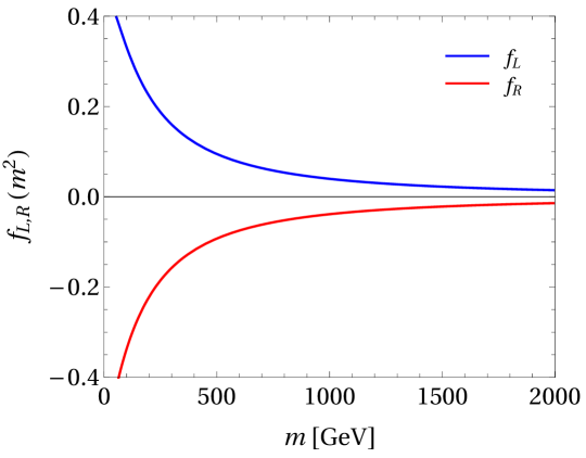
Figure 2: The functions $f_{L}\left(m^{2}\right)$ and $f_{R}\left(m^{2}\right)$.

One sees that $f_{L}\left(m^{2}\right)>0$, $f_{R}\left(m^{2}\right)<0$, and $f_{R}\left(m^{2}\right)\approx-f_{L}\left(m^{2}\right)$ for all values of $m^{2}$. Moreover, the absolute values of both functions decrease with increasing $m^{2}$. Therefore, $\delta g_{L}^{c}>0$, $\delta g_{R}^{c}<0$, and both $\delta g_{L}^{c}$ and $-\delta g_{R}^{c}$ are monotonically decreasing functions of the charged-scalar masses.

2.4 The neutral-scalar contribution

The neutral-scalar contribution to $\delta g_{L}$ and $\delta g_{R}$ has been recently emphasized in ref. [15], following the original computation in ref. [3]; it corresponds to the computation of the diagrams in figure 3

Figure 3: Feynman diagrams that produce equations (24) and (25).

and it is recapitulated in appendix B.

Figure 4: Feynman diagrams that do not contribute to $\delta g_{L}$ and $\delta g_{R}$ in the specific case of this paper.

Assuming alignment and discarding the Standard-Model contributions that involve $S_{1}^{0}$ and $S_{2}^{0}$, one has

$$\delta g_{L}^{n} = \frac{1}{16\pi^{2}}\sum_{j=3}^{2n-1}\sum_{j^{\prime}=j+1}^{2n}\mathcal{A}_{jj^{\prime}}\ \mathrm{Im}\left[\left(\mathcal{V}^{\dagger}\mathcal{F}^{\ast}\right)_{j}\left(\mathcal{V}^{T}\mathcal{F}\right)_{j^{\prime}}\right]h_{L}\left(m_{j}^{2},\,m_{j^{\prime}}^{2}\right),$$ (24a)

$$\delta g_{R}^{n} = \frac{1}{16\pi^{2}}\sum_{j=3}^{2n-1}\sum_{j^{\prime}=j+1}^{2n}\mathcal{A}_{jj^{\prime}}\ \mathrm{Im}\left[\left(\mathcal{V}^{\dagger}\mathcal{F}^{\ast}\right)_{j}\left(\mathcal{V}^{T}\mathcal{F}\right)_{j^{\prime}}\right]h_{R}\left(m_{j}^{2},\,m_{j^{\prime}}^{2}\right),$$ (24b)

where $\mathcal{F}$ is an $n\times 1$ vector with $k^{\mathrm{th}}$ component $\mathcal{F}_{k}=f_{k}$ for $k=2,\ldots,n$, and

$$h_{L}\left(m_{j}^{2},\,m_{j^{\prime}}^{2}\right) = -C_{00}\left(0,\,m_{Z}^{2},\,0,\,0,\,m_{j}^{2},\,m_{j^{\prime}}^{2}\right)$$ (25a)

$$+\frac{s_{w}^{2}}{6}\left[2\,C_{00}\left(0,\,m_{Z}^{2},\,0,\,m_{j}^{2},\,0,\,0\right)+2\,C_{00}\left(0,\,m_{Z}^{2},\,0,\,m_{j^{\prime}}^{2},\,0,\,0\right)\right.$$

$$\left.-1-m_{Z}^{2}\,C_{12}\left(0,\,m_{Z}^{2},\,0,\,m_{j}^{2},\,0,\,0\right)-m_{Z}^{2}\,C_{12}\left(0,\,m_{Z}^{2},\,0,\,m_{j^{\prime}}^{2},\,0,\,0\right)\right]$$

$$+\left(\frac{s_{w}^{2}}{6}-\frac{1}{4}\right)\left[B_{1}\left(0,\,0,\,m_{j}^{2}\right)+B_{1}\left(0,\,0,\,m_{j^{\prime}}^{2}\right)\right],$$

$$h_{R}\left(m_{j}^{2},\,m_{j^{\prime}}^{2}\right) = C_{00}\left(0,\,m_{Z}^{2},\,0,\,0,\,m_{j}^{2},\,m_{j^{\prime}}^{2}\right)$$ (25b)

$$+\left(\frac{s_{w}^{2}}{6}-\frac{1}{4}\right)\left[2\,C_{00}\left(0,\,m_{Z}^{2},\,0,\,m_{j}^{2},\,0,\,0\right)+2\,C_{00}\left(0,\,m_{Z}^{2},\,0,\,m_{j^{\prime}}^{2},\,0,\,0\right)\right.$$

$$\left.-1-m_{Z}^{2}\,C_{12}\left(0,\,m_{Z}^{2},\,0,\,m_{j}^{2},\,0,\,0\right)-m_{Z}^{2}\,C_{12}\left(0,\,m_{Z}^{2},\,0,\,m_{j^{\prime}}^{2},\,0,\,0\right)\right]$$

$$+\frac{s_{w}^{2}}{6}\left[B_{1}\left(0,\,0,\,m_{j}^{2}\right)+B_{1}\left(0,\,0,\,m_{j^{\prime}}^{2}\right)\right].$$

The functions $h_{L}$ and $h_{R}$ are independent of $s_{w}$ when $m_{Z}=0$; however, that approximation is not a good one for those functions. We depict their real parts in figure 5.

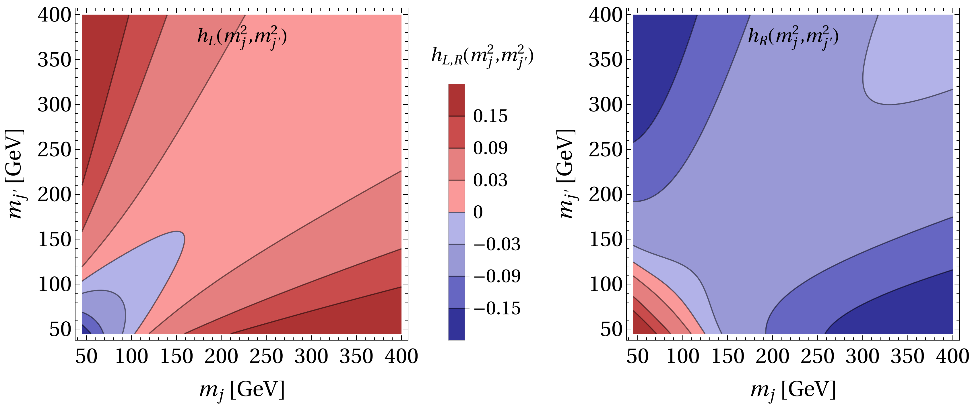
Figure 5: The functions $h_{L}\left(m_{j}^{2},\,m_{j^{\prime}}^{2}\right)$ and $h_{R}\left(m_{j}^{2},\,m_{j^{\prime}}^{2}\right)$.

One sees that, when both $m_{j}$ and $m_{j^{\prime}}$ are larger than the Fermi scale, $h_{L}\left(m_{j}^{2},\,m_{j^{\prime}}^{2}\right)>0$ and $h_{R}\left(m_{j}^{2},\,m_{j^{\prime}}^{2}\right)<0$. However, if both $m_{j}\lesssim 100$ GeV and $m_{j^{\prime}}\lesssim 100$ GeV, then both $h_{L}\left(m_{j}^{2},\,m_{j^{\prime}}^{2}\right)$ and $h_{R}\left(m_{j}^{2},\,m_{j^{\prime}}^{2}\right)$ invert their usual signs. Moreover, $\left|h_{L}\left(m_{j}^{2},\,m_{j^{\prime}}^{2}\right)\right|$ and $\left|h_{R}\left(m_{j}^{2},\,m_{j^{\prime}}^{2}\right)\right|$ become rather large either when $\left|m_{j}-m_{j^{\prime}}\right|\gtrsim 200$ GeV and one of the masses $\lesssim 50$ GeV, or when both $m_{j}$ and $m_{j^{\prime}}\lesssim 50$ GeV.

3 The aligned 2HDM

In a two-Higgs-doublet model with alignment [15], the doublet $\Phi_{2}$ may be rephased so that $R_{2}\equiv S_{3}^{0}$ and $I_{2}\equiv S_{4}^{0}$ are the new physical neutral scalars. Then,

$$\mathcal{V}=\left(\begin{array}[]{cccc}i&1&0&0\\ 0&0&1&i\end{array}\right),$$ (26)

hence $\mathcal{A}_{34}=1$ and $\left(\mathcal{V}^{\dagger}\mathcal{F}^{\ast}\right)_{3}\left(\mathcal{V}^{T}\mathcal{F}\right)_{4}=i\left|f_{2}\right|^{2}$. There are five New-Physics parameters on which $\delta g_{L}$ and $\delta g_{R}$ depend: the neutral-scalar masses $m_{3}$ and $m_{4}$, the charged-scalar mass $m_{C2}$, and the Yukawa couplings $e_{2}$ and $f_{2}$. One has [15]

$$\delta g_{L} = \frac{\left|e_{2}\right|^{2}f_{L}\left(m_{C2}^{2}\right)+\left|f_{2}\right|^{2}h_{L}\left(m_{3}^{2},\,m_{4}^{2}\right)}{16\pi^{2}},$$ (27a)

$$\delta g_{R} = \frac{\left|f_{2}\right|^{2}\left[f_{R}\left(m_{C2}^{2}\right)+h_{R}\left(m_{3}^{2},\,m_{4}^{2}\right)\right]}{16\pi^{2}}.$$ (27b)

We now consider the scalar potential of the 2HDM [18],

$$V = \mu_{1}\,\Phi_{1}^{\dagger}\Phi_{1}+\mu_{2}\,\Phi_{2}^{\dagger}\Phi_{2}+\left(\mu_{3}\,\Phi_{1}^{\dagger}\Phi_{2}+\mathrm{H.c.}\right)$$ (28)

$$+\frac{\lambda_{1}}{2}\left(\Phi_{1}^{\dagger}\Phi_{1}\right)^{2}+\frac{\lambda_{2}}{2}\left(\Phi_{2}^{\dagger}\Phi_{2}\right)^{2}+\lambda_{3}\,\Phi_{1}^{\dagger}\Phi_{1}\,\Phi_{2}^{\dagger}\Phi_{2}+\lambda_{4}\,\Phi_{1}^{\dagger}\Phi_{2}\,\Phi_{2}^{\dagger}\Phi_{1}$$

$$+\left[\frac{\lambda_{5}}{2}\left(\Phi_{1}^{\dagger}\Phi_{2}\right)^{2}+\lambda_{6}\,\Phi_{1}^{\dagger}\Phi_{1}\,\Phi_{1}^{\dagger}\Phi_{2}+\lambda_{7}\,\Phi_{2}^{\dagger}\Phi_{2}\,\Phi_{1}^{\dagger}\Phi_{2}+\mathrm{H.c.}\right].$$

In the Higgs basis, $\mu_{1}=-\left.\lambda_{1}v^{2}\right/2$ and $\mu_{3}=-\left.\lambda_{6}v^{2}\right/2$. Because of alignment, $\lambda_{6}$ (and $\mu_{3}$) are zero and

$$\lambda_{1}=\frac{m_{2}^{2}}{v^{2}}=\left(\frac{125\,\mathrm{GeV}}{246\,\mathrm{GeV}}\right)^{2}\approx 0.258.$$ (29)

From the masses of the scalars we compute

$$\lambda_{4}=\frac{m_{3}^{2}+m_{4}^{2}-2m_{C2}^{2}}{v^{2}},\quad\Lambda_{5}=\frac{m_{4}^{2}-m_{3}^{2}}{v^{2}},$$ (30)

where $\Lambda_{5}:=\left|\lambda_{5}\right|$.

The masses $m_{C2}$, $m_{3}$, and $m_{4}$ are not completely free, because they must comply with unitarity (UNI) and bounded-from-below (BFB) requirements [18]. For the sake of simplicity, in our analysis we assume $\lambda_{2}=\lambda_{7}=0$. We enforce the UNI conditions

$$\lambda_{4}^{2}<64\pi^{2}-8\pi\lambda_{1},\quad\Lambda_{5}^{2}<64\pi^{2}-8\pi\lambda_{1}$$ (31)

on the quantities (30). Additionally, there are

• BFB conditions [18]

  $$\lambda_{3}>0,\quad\lambda_{3}+\lambda_{4}-\Lambda_{5}>0;$$ (32)

• UNI conditions [18]

  $$\begin{array}[]{lcl}\left|\lambda_{3}\right|+\left|\lambda_{4}\right|<8\pi,&&\left|\lambda_{3}\right|+\Lambda_{5}<8\pi,\\[2.84526pt] \left|\lambda_{3}+2\lambda_{4}\right|+3\Lambda_{5}<8\pi,&&\left(2\lambda_{3}+\lambda_{4}\right)^{2}<64\pi^{2}-24\pi\lambda_{1};\end{array}$$ (33)

• the condition to avoid the situation of ‘panic vacuum’, namely [19]

  $$\left[\left(\frac{m_{C2}^{2}}{v^{2}}+\frac{\lambda_{4}}{2}\right)^{2}-\frac{\Lambda_{5}^{2}}{4}\right]\left(\frac{m_{C2}^{2}}{v^{2}}-\frac{\lambda_{3}}{2}\right)>0.$$ (34)

After computing $\lambda_{4}$ and $\Lambda_{5}$ through equations (30) and after checking inequalities (31), we verify whether there is any value of $\lambda_{3}$ that satisfies the inequalities (32)–(34); if there is, then the inputed masses $m_{C2}$, $m_{3}$, and $m_{4}$ are valid; else, they are not.

We also compute the contribution of the new scalars to the oblique parameter

$$T=\frac{1}{16\pi s_{w}^{2}m_{W}^{2}}\left[F\left(m_{C2}^{2},\ m_{3}^{2}\right)+F\left(m_{C2}^{2},\ m_{4}^{2}\right)-F\left(m_{3}^{2},\ m_{4}^{2}\right)\right],$$ (35)

where $m_{W}=80.4$ GeV is the mass of the gauge bosons $W^{\pm}$ and

$$F\left(A,\,B\right)=\left\{\begin{array}[]{lcl}\displaystyle{\frac{A+B}{2}-\frac{AB}{A-B}\,\ln{\frac{A}{B}}}&\Leftarrow&A\neq B,\\[8.53581pt] 0&\Leftarrow&A=B.\end{array}\right.$$ (36)

Additionally, we apply constraints on the oblique parameter [20]

$$S=\frac{4s_{w}^{2}c_{w}^{2}}{\alpha}\left[\left.\frac{\partial A_{ZZ}\left(q^{2}\right)}{\partial q^{2}}\right|_{q^{2}=m_{Z}^{2}}-\left.\frac{\partial A_{\gamma\gamma}\left(q^{2}\right)}{\partial q^{2}}\right|_{q^{2}=0}+\frac{c_{w}^{2}-s_{w}^{2}}{c_{w}s_{w}}\left.\frac{\partial A_{\gamma Z}\left(q^{2}\right)}{\partial q^{2}}\right|_{q^{2}=0}\right].$$ (37)

This parameter has been computed in ref. [21] to be

$$S=\frac{1}{24\pi}\left[\ln{\frac{m_{3}^{2}m_{4}^{2}}{m_{C2}^{4}}}+\left(s_{w}^{2}-c_{w}^{2}\right)^{2}f\left(m_{C2}^{2},\,m_{C2}^{2},\,m_{Z}^{2}\right)+f\left(m_{3}^{2},\,m_{4}^{2},\,m_{Z}^{2}\right)\right].$$ (38)

Here,

$$f\left(A,\,B,\,C\right) = -\frac{10}{3}-4\,\frac{A+B}{C}+4\,\frac{\left(A-B\right)^{2}}{C^{2}}+\left[3\,\frac{A^{2}-B^{2}}{C^{2}}-2\,\frac{\left(A-B\right)^{3}}{C^{3}}\right]\ln{\frac{A}{B}}\hskip 19.91692pt$$ (39b)

$$+\left[\frac{1}{C}+\frac{A+B}{C^{2}}-2\,\frac{\left(A-B\right)^{2}}{C^{3}}\right]h\left(t,\,r\right),$$

where $t\equiv A+B-C$, $r\equiv A^{2}+B^{2}+C^{2}-2\left(AB+AC+BC\right)$, and

$$h\left(t,\,r\right)=\left\{\begin{array}[]{lcl}{\displaystyle\sqrt{r}\,\ln{\left|\frac{t-\sqrt{r}}{t+\sqrt{r}}\right|}}&\Leftarrow&r>0,\\ 0&\Leftarrow&r=0,\\ {\displaystyle 2\,\sqrt{-r}\,\arctan{\frac{\sqrt{-r}}{t}}}&\Leftarrow&r<0.\end{array}\right.$$ (40)

We either enforce the phenomenological constraint [1]

$$T = 0.03\pm 0.12,$$ (41a)

$$S = -0.01\pm 0.10$$ (41b)

or we allow for other New Physics beyond the 2HDM and apply milder requirements by allowing values of $T$ and $S$ within its $3\sigma$ and $2\sigma$ bounds, respectively.

4 The aligned 3HDM

4.1 Parameterization of the neutral-scalar mixing

In the three-Higgs-doublet model with alignment,

$$\left(\begin{array}[]{c}R_{2}\\ R_{3}\\ I_{2}\\ I_{3}\end{array}\right)=\mathcal{T}\left(\begin{array}[]{c}S_{3}^{0}\\ S_{4}^{0}\\ S_{5}^{0}\\ S_{6}^{0}\end{array}\right),$$ (42)

where $\mathcal{T}$ is a $4\times 4$ real orthogonal matrix. We parameterize

$$\mathcal{T}=\mathcal{O}_{13}\left(\theta_{5}\right)\times\mathcal{O}_{24}\left(\theta_{6}\right)\times\mathcal{O}_{12}\left(\theta_{1}\right)\times\mathcal{O}_{34}\left(\theta_{2}\right)\times\mathcal{O}_{14}\left(\theta_{3}\right)\times\mathcal{O}_{23}\left(\theta_{4}\right),$$ (43)

where $\mathcal{O}_{pq}\left(\theta\right)$ represents a rotation through an angle $\theta$ in the $\left(p,\,q\right)$ plane. Now, $\mathcal{O}_{13}\left(\theta_{5}\right)$ is a rotation that mixes $R_{2}$ and $I_{2}$, and $\mathcal{O}_{24}\left(\theta_{6}\right)$ is a rotation mixing $R_{3}$ and $I_{3}$, viz. they represent rephasings of the doublets $\Phi_{2}$ and $\Phi_{3}$, respectively. Since such rephasings are unphysical, one may without loss of generality drop those two rotations from the parameterization (43), obtaining

$$\mathcal{T}=\left(\begin{array}[]{cccc}c_{1}c_{3}&-s_{1}c_{4}&s_{1}s_{4}&-c_{1}s_{3}\\ s_{1}c_{3}&c_{1}c_{4}&-c_{1}s_{4}&-s_{1}s_{3}\\ -s_{2}s_{3}&c_{2}s_{4}&c_{2}c_{4}&-s_{2}c_{3}\\ c_{2}s_{3}&s_{2}s_{4}&s_{2}c_{4}&c_{2}c_{3}\end{array}\right),$$ (44)

where $c_{p}=\cos{\theta_{p}}$ and $s_{p}=\sin{\theta_{p}}$ for $p=1,2,3,4$. Then,

$$\delta g_{L} = \frac{\left|e_{2}\right|^{2}f_{L}\left(m_{C2}^{2}\right)+\left|e_{3}\right|^{2}f_{L}\left(m_{C3}^{2}\right)}{16\pi^{2}}$$ (45a)

$$+\frac{1}{16\pi^{2}}\sum_{j=3}^{5}\sum_{j^{\prime}=j+1}^{6}\mathcal{A}_{jj^{\prime}}\ \mathrm{Im}\left[\left(\mathcal{V}^{\dagger}\mathcal{F}^{\ast}\right)_{j}\left(\mathcal{V}^{T}\mathcal{F}\right)_{j^{\prime}}\right]h_{L}\left(m_{j}^{2},\,m_{j^{\prime}}^{2}\right),$$

$$\delta g_{R} = \frac{\left|f_{2}\right|^{2}f_{R}\left(m_{C2}^{2}\right)+\left|f_{3}\right|^{2}f_{R}\left(m_{C3}^{2}\right)}{16\pi^{2}}$$ (45b)

$$+\frac{1}{16\pi^{2}}\sum_{j=3}^{5}\sum_{j^{\prime}=j+1}^{6}\mathcal{A}_{jj^{\prime}}\ \mathrm{Im}\left[\left(\mathcal{V}^{\dagger}\mathcal{F}^{\ast}\right)_{j}\left(\mathcal{V}^{T}\mathcal{F}\right)_{j^{\prime}}\right]h_{R}\left(m_{j}^{2},\,m_{j^{\prime}}^{2}\right),$$

with

$$\mathcal{A}_{34}=-\mathcal{A}_{56} = \left(c_{1}c_{2}+s_{1}s_{2}\right)\left(c_{3}s_{4}-s_{3}c_{4}\right),$$ (46a)

$$\mathcal{A}_{35}=\mathcal{A}_{46} = \left(c_{1}c_{2}+s_{1}s_{2}\right)\left(c_{3}c_{4}+s_{3}s_{4}\right),$$ (46b)

$$\mathcal{A}_{36}=-\mathcal{A}_{45} = s_{1}c_{2}-c_{1}s_{2},$$ (46c)

and

$$\mathrm{Im}\left[\left(\mathcal{V}^{\dagger}\mathcal{F}^{\ast}\right)_{3}\left(\mathcal{V}^{T}\mathcal{F}\right)_{4}\right] = \left|f_{2}\right|^{2}\left(c_{1}c_{2}c_{3}s_{4}-s_{1}s_{2}s_{3}c_{4}\right)+\left|f_{3}\right|^{2}\left(s_{1}s_{2}c_{3}s_{4}-c_{1}c_{2}s_{3}c_{4}\right)$$ (47a)

$$+\mathrm{Re}\left(f_{2}f_{3}^{\ast}\right)\left(c_{1}s_{2}+s_{1}c_{2}\right)\left(c_{3}s_{4}+s_{3}c_{4}\right)$$

$$+\mathrm{Im}\left(f_{2}f_{3}^{\ast}\right)\left(s_{3}s_{4}-c_{3}c_{4}\right),$$

$$\mathrm{Im}\left[\left(\mathcal{V}^{\dagger}\mathcal{F}^{\ast}\right)_{3}\left(\mathcal{V}^{T}\mathcal{F}\right)_{5}\right] = \left|f_{2}\right|^{2}\left(c_{1}c_{2}c_{3}c_{4}+s_{1}s_{2}s_{3}s_{4}\right)+\left|f_{3}\right|^{2}\left(s_{1}s_{2}c_{3}c_{4}+c_{1}c_{2}s_{3}s_{4}\right)$$ (47b)

$$+\mathrm{Re}\left(f_{2}f_{3}^{\ast}\right)\left(c_{1}s_{2}+s_{1}c_{2}\right)\left(c_{3}c_{4}-s_{3}s_{4}\right)$$

$$+\mathrm{Im}\left(f_{2}f_{3}^{\ast}\right)\left(c_{3}s_{4}+s_{3}c_{4}\right),$$

$$\mathrm{Im}\left[\left(\mathcal{V}^{\dagger}\mathcal{F}^{\ast}\right)_{3}\left(\mathcal{V}^{T}\mathcal{F}\right)_{6}\right] = -c_{1}s_{2}\left|f_{2}\right|^{2}+s_{1}c_{2}\left|f_{3}\right|^{2}+\mathrm{Re}\left(f_{2}f_{3}^{\ast}\right)\left(c_{1}c_{2}-s_{1}s_{2}\right),$$ (47c)

$$\mathrm{Im}\left[\left(\mathcal{V}^{\dagger}\mathcal{F}^{\ast}\right)_{4}\left(\mathcal{V}^{T}\mathcal{F}\right)_{5}\right] = -s_{1}c_{2}\left|f_{2}\right|^{2}+c_{1}s_{2}\left|f_{3}\right|^{2}+\mathrm{Re}\left(f_{2}f_{3}^{\ast}\right)\left(c_{1}c_{2}-s_{1}s_{2}\right),$$ (47d)

$$\mathrm{Im}\left[\left(\mathcal{V}^{\dagger}\mathcal{F}^{\ast}\right)_{4}\left(\mathcal{V}^{T}\mathcal{F}\right)_{6}\right] = \left|f_{2}\right|^{2}\left(s_{1}s_{2}c_{3}c_{4}+c_{1}c_{2}s_{3}s_{4}\right)+\left|f_{3}\right|^{2}\left(c_{1}c_{2}c_{3}c_{4}+s_{1}s_{2}s_{3}s_{4}\right)$$ (47e)

$$-\mathrm{Re}\left(f_{2}f_{3}^{\ast}\right)\left(c_{1}s_{2}+s_{1}c_{2}\right)\left(c_{3}c_{4}-s_{3}s_{4}\right),$$

$$-\mathrm{Im}\left(f_{2}f_{3}^{\ast}\right)\left(c_{3}s_{4}+s_{3}c_{4}\right),$$

$$\mathrm{Im}\left[\left(\mathcal{V}^{\dagger}\mathcal{F}^{\ast}\right)_{5}\left(\mathcal{V}^{T}\mathcal{F}\right)_{6}\right] = \left|f_{2}\right|^{2}\left(c_{1}c_{2}s_{3}c_{4}-s_{1}s_{2}c_{3}s_{4}\right)+\left|f_{3}\right|^{2}\left(s_{1}s_{2}s_{3}c_{4}-c_{1}c_{2}c_{3}s_{4}\right)$$ (47f)

$$+\mathrm{Re}\left(f_{2}f_{3}^{\ast}\right)\left(c_{1}s_{2}+s_{1}c_{2}\right)\left(c_{3}s_{4}+s_{3}c_{4}\right),$$

$$+\mathrm{Im}\left(f_{2}f_{3}^{\ast}\right)\left(s_{3}s_{4}-c_{3}c_{4}\right).$$

The contribution of the new scalars to the oblique parameter $T$, given in equation (23) of ref. [22], is

$$T = \frac{1}{16\pi s_{w}^{2}m_{W}^{2}}\left\{\left(c_{1}^{2}c_{3}^{2}+s_{2}^{2}s_{3}^{2}\right)F\left(m_{C2}^{2},\,m_{3}^{2}\right)+\left(s_{1}^{2}c_{4}^{2}+c_{2}^{2}s_{4}^{2}\right)F\left(m_{C2}^{2},\,m_{4}^{2}\right)\right.$$ (48)

$$\hskip 51.21495pt+\left(s_{1}^{2}s_{4}^{2}+c_{2}^{2}c_{4}^{2}\right)F\left(m_{C2}^{2},\,m_{5}^{2}\right)+\left(c_{1}^{2}s_{3}^{2}+s_{2}^{2}c_{3}^{2}\right)F\left(m_{C2}^{2},\,m_{6}^{2}\right)$$

$$\hskip 51.21495pt+\left(s_{1}^{2}c_{3}^{2}+c_{2}^{2}s_{3}^{2}\right)F\left(m_{C3}^{2},\,m_{3}^{2}\right)+\left(c_{1}^{2}c_{4}^{2}+s_{2}^{2}s_{4}^{2}\right)F\left(m_{C3}^{2},\,m_{4}^{2}\right)$$

$$\hskip 51.21495pt+\left(c_{1}^{2}s_{4}^{2}+s_{2}^{2}c_{4}^{2}\right)F\left(m_{C3}^{2},\,m_{5}^{2}\right)+\left(s_{1}^{2}s_{3}^{2}+c_{2}^{2}c_{3}^{2}\right)F\left(m_{C3}^{2},\,m_{6}^{2}\right)$$

$$\hskip 51.21495pt-\left(\mathcal{A}_{34}\right)^{2}\left[F\left(m_{3}^{2},\,m_{4}^{2}\right)+F\left(m_{5}^{2},\,m_{6}^{2}\right)\right]$$

$$\hskip 51.21495pt-\left(\mathcal{A}_{35}\right)^{2}\left[F\left(m_{3}^{2},\,m_{5}^{2}\right)+F\left(m_{4}^{2},\,m_{6}^{2}\right)\right]$$

$$\left.\hskip 51.21495pt-\left(\mathcal{A}_{36}\right)^{2}\left[F\left(m_{3}^{2},\,m_{6}^{2}\right)+F\left(m_{4}^{2},\,m_{5}^{2}\right)\right]\right\}.$$

For the oblique parameter $S$ one has

$$S = \frac{1}{24\pi}\left\{\left(s_{w}^{2}-c_{w}^{2}\right)^{2}\left[f\left(m_{C2}^{2},\,m_{C2}^{2},\,m_{Z}^{2}\right)+f\left(m_{C3}^{2},\,m_{C3}^{2},\,m_{Z}^{2}\right)\right]\right.$$ (49d)

$$+\ln{\frac{m_{3}^{2}m_{4}^{2}m_{5}^{2}m_{6}^{2}}{m_{C2}^{4}m_{C3}^{4}}}+\left(\mathcal{A}_{34}\right)^{2}\left[f\left(m_{3}^{2},\,m_{4}^{2},\,m_{Z}^{2}\right)+f\left(m_{5}^{2},\,m_{6}^{2},\,m_{Z}^{2}\right)\right]$$

$$+\left(\mathcal{A}_{35}\right)^{2}\left[f\left(m_{3}^{2},\,m_{5}^{2},\,m_{Z}^{2}\right)+f\left(m_{4}^{2},\,m_{6}^{2},\,m_{Z}^{2}\right)\right]$$

$$\left.+\left(\mathcal{A}_{45}\right)^{2}\left[f\left(m_{3}^{2},\,m_{6}^{2},\,m_{Z}^{2}\right)+f\left(m_{4}^{2},\,m_{5}^{2},\,m_{Z}^{2}\right)\right]\right\}.$$

4.2 The scalar potential

The parameters

The scalar potential of the 3HDM has lots of couplings and it is impractical to work with it. So we concentrate on a truncated version of the potential, viz. we discard from the quartic part of the potential all the terms that either do not contain $\Phi_{1}$ or are linear in $\Phi_{1}$. The remaining potential is

$$V = \mu_{1}\,\Phi_{1}^{\dagger}\Phi_{1}+\mu_{2}\,\Phi_{2}^{\dagger}\Phi_{2}+\mu_{3}\,\Phi_{3}^{\dagger}\Phi_{3}+\left(\mu_{4}\,\Phi_{1}^{\dagger}\Phi_{2}+\mu_{5}\,\Phi_{1}^{\dagger}\Phi_{3}+\mu_{6}\,\Phi_{2}^{\dagger}\Phi_{3}+\mathrm{H.c.}\right)$$ (50)

$$+\frac{\lambda_{1}}{2}\left(\Phi_{1}^{\dagger}\Phi_{1}\right)^{2}+\lambda_{4}\,\Phi_{1}^{\dagger}\Phi_{1}\,\Phi_{2}^{\dagger}\Phi_{2}+\lambda_{5}\,\Phi_{1}^{\dagger}\Phi_{1}\,\Phi_{3}^{\dagger}\Phi_{3}+\lambda_{7}\,\Phi_{1}^{\dagger}\Phi_{2}\,\Phi_{2}^{\dagger}\Phi_{1}+\lambda_{8}\,\Phi_{1}^{\dagger}\Phi_{3}\,\Phi_{3}^{\dagger}\Phi_{1}$$

$$+\left[\frac{\lambda_{10}}{2}\left(\Phi_{1}^{\dagger}\Phi_{2}\right)^{2}+\frac{\lambda_{11}}{2}\left(\Phi_{1}^{\dagger}\Phi_{3}\right)^{2}+\lambda_{13}\,\Phi_{1}^{\dagger}\Phi_{1}\,\Phi_{1}^{\dagger}\Phi_{2}+\lambda_{14}\,\Phi_{1}^{\dagger}\Phi_{1}\,\Phi_{1}^{\dagger}\Phi_{3}\right.$$

$$\left.+\lambda_{19}\,\Phi_{1}^{\dagger}\Phi_{1}\,\Phi_{2}^{\dagger}\Phi_{3}+\lambda_{22}\,\Phi_{1}^{\dagger}\Phi_{3}\,\Phi_{2}^{\dagger}\Phi_{1}+\lambda_{25}\,\Phi_{1}^{\dagger}\Phi_{2}\,\Phi_{1}^{\dagger}\Phi_{3}+\mathrm{H.c.}\vphantom{\frac{\lambda_{10}}{2}}\right],$$

where $\mu_{1,2,3}$ and $\lambda_{1,4,5,7,8}$ are real and the remaining parameters are in general complex. In order that the VEV of $\Phi_{1}$ is $v\left/\sqrt{2}\right.$ and the VEVs of $\Phi_{2}$ and $\Phi_{3}$ are zero, one must have

$$\mu_{1}=-\frac{\lambda_{1}v^{2}}{2},\quad\mu_{4}=-\frac{\lambda_{13}v^{2}}{2},\quad\mu_{5}=-\frac{\lambda_{14}v^{2}}{2}.$$ (51)

In order that the charged-scalar mass matrix is $\mathrm{diag}\left(m_{C2}^{2},\,m_{C3}^{2}\right)$, one must have

$$\mu_{2}=m_{C2}^{2}-\frac{\lambda_{4}v^{2}}{2},\quad\mu_{3}=m_{C3}^{2}-\frac{\lambda_{5}v^{2}}{2},\quad\mu_{6}=-\frac{\lambda_{19}v^{2}}{2}.$$ (52)

Equations (51) and (52) are the conditions for the charged Higgs basis. Next we write down the conditions for alignment, i.e. for $H\equiv S_{2}^{0}$ to have mass $m_{2}$ and not to have mass terms together with either $R_{2}$, $R_{3}$, $I_{2}$, or $I_{3}$:

$$\lambda_{1}=\frac{m_{2}^{2}}{v^{2}}\approx 0.258,\quad\lambda_{13}=\lambda_{14}=0,$$ (53)

hence $\mu_{4}$ and $\mu_{5}$ are zero too. The mass terms of $R_{2}$, $R_{3}$, $I_{2}$, and $I_{3}$ are given by

$$V=\cdots+\frac{1}{2}\left(\begin{array}[]{cccc}R_{2},&R_{3},&I_{2},&I_{3}\end{array}\right)N\left(\begin{array}[]{c}R_{2}\\ R_{3}\\ I_{2}\\ I_{3}\end{array}\right),$$ (54)

where $N$ is a $4\times 4$ real symmetric matrix. Using equations (42) and (44), one finds that

$$N_{11}-m_{C2}^{2}$$

$$=\frac{v^{2}}{2}\left(\lambda_{7}+\mathrm{Re}\,\lambda_{10}\right) = m_{3}^{2}c_{1}^{2}c_{3}^{2}+m_{4}^{4}s_{1}^{2}c_{3}^{2}+m_{5}^{2}s_{2}^{2}s_{3}^{2}+m_{6}^{2}c_{2}^{2}s_{3}^{2}-m_{C2}^{2},$$ (55a)

$$N_{33}-m_{C2}^{2}$$

$$=\frac{v^{2}}{2}\left(\lambda_{7}-\mathrm{Re}\,\lambda_{10}\right) = m_{3}^{2}s_{1}^{2}s_{4}^{2}+m_{4}^{4}c_{1}^{2}s_{4}^{2}+m_{5}^{2}c_{2}^{2}c_{4}^{2}+m_{6}^{2}s_{2}^{2}c_{4}^{2}-m_{C2}^{2},$$ (55b)

$$N_{13}=-\frac{v^{2}}{2}\,\mathrm{Im}\,\lambda_{10} = \left(m_{3}^{2}-m_{4}^{2}\right)c_{1}s_{1}c_{3}s_{4}+\left(m_{6}^{2}-m_{5}^{2}\right)c_{2}s_{2}s_{3}c_{4},$$ (55c)

$$N_{22}-m_{C3}^{2}$$

$$=\frac{v^{2}}{2}\left(\lambda_{8}+\mathrm{Re}\,\lambda_{11}\right) = m_{3}^{2}s_{1}^{2}c_{4}^{2}+m_{4}^{4}c_{1}^{2}c_{4}^{2}+m_{5}^{2}c_{2}^{2}s_{4}^{2}+m_{6}^{2}s_{2}^{2}s_{4}^{2}-m_{C3}^{2},$$ (55d)

$$N_{44}-m_{C3}^{2}$$

$$=\frac{v^{2}}{2}\left(\lambda_{8}-\mathrm{Re}\,\lambda_{11}\right) = m_{3}^{2}c_{1}^{2}s_{3}^{2}+m_{4}^{4}s_{1}^{2}s_{3}^{2}+m_{5}^{2}s_{2}^{2}c_{3}^{2}+m_{6}^{2}c_{2}^{2}c_{3}^{2}-m_{C3}^{2},$$ (55e)

$$N_{24}=-\frac{v^{2}}{2}\,\mathrm{Im}\,\lambda_{11} = \left(m_{3}^{2}-m_{4}^{2}\right)c_{1}s_{1}s_{3}c_{4}+\left(m_{6}^{2}-m_{5}^{2}\right)c_{2}s_{2}c_{3}s_{4},$$ (55f)

$$N_{12}=\frac{v^{2}}{2}\,\mathrm{Re}\left(\lambda_{22}+\lambda_{25}\right) = \left(m_{4}^{2}-m_{3}^{2}\right)c_{1}s_{1}c_{3}c_{4}+\left(m_{6}^{2}-m_{5}^{2}\right)c_{2}s_{2}s_{3}s_{4},$$ (55g)

$$N_{34}=\frac{v^{2}}{2}\,\mathrm{Re}\left(\lambda_{22}-\lambda_{25}\right) = \left(m_{4}^{2}-m_{3}^{2}\right)c_{1}s_{1}s_{3}s_{4}+\left(m_{6}^{2}-m_{5}^{2}\right)c_{2}s_{2}c_{3}c_{4},$$ (55h)

$$N_{14}=-\frac{v^{2}}{2}\,\mathrm{Im}\left(\lambda_{22}+\lambda_{25}\right) = c_{3}s_{3}\left(-c_{1}^{2}m_{3}^{2}-s_{1}^{2}m_{4}^{2}+s_{2}^{2}m_{5}^{2}+c_{2}^{2}m_{6}^{2}\right),$$ (55i)

$$N_{23}=\frac{v^{2}}{2}\,\mathrm{Im}\left(\lambda_{22}-\lambda_{25}\right) = c_{4}s_{4}\left(-s_{1}^{2}m_{3}^{2}-c_{1}^{2}m_{4}^{2}+c_{2}^{2}m_{5}^{2}+s_{2}^{2}m_{6}^{2}\right).$$ (55j)

Equations (55) allow one to compute $\lambda_{7}$, $\lambda_{8}$, $\lambda_{10}$, $\lambda_{11}$, $\lambda_{22}$, and $\lambda_{25}$ by using as input the masses of the charged scalars and the masses and mixings of the neutral scalars. On the other hand, $\lambda_{4}$, $\lambda_{5}$, and $\lambda_{19}$ constitute extra parameters that we input by hand—just as we did with $\lambda_{3}$ in section 3.

UNI constraints

These constraints state that the moduli of the eigenvalues of some matrices must be smaller than $8\pi$. The method for the derivation of those matrices in a general $n$HDM was explained in ref. [14]. In our specific case, the UNI constraints are (using $\Lambda_{i}\equiv\left|\lambda_{i}\right|$ for $i=10,11,19,22,25$),

$$\left|\lambda_{4}+\lambda_{5}-\lambda_{7}-\lambda_{8}\right|+\sqrt{\left(\lambda_{4}-\lambda_{5}-\lambda_{7}+\lambda_{8}\right)^{2}+4\left|\lambda_{19}-\lambda_{22}\right|^{2}} < 16\pi,$$ (56a)

$$\left|\lambda_{4}+\lambda_{5}+\lambda_{7}+\lambda_{8}\right|+\sqrt{\left(\lambda_{4}-\lambda_{5}+\lambda_{7}-\lambda_{8}\right)^{2}+4\left|\lambda_{19}+\lambda_{22}\right|^{2}} < 16\pi,$$ (56b)

$$\lambda_{1}+\sqrt{\lambda_{1}^{2}+4\left(\Lambda_{10}^{2}+\Lambda_{11}^{2}+2\Lambda_{25}^{2}\right)} < 16\pi,$$ (56c)

$$\lambda_{1}+\sqrt{\lambda_{1}^{2}+4\left(\lambda_{7}^{2}+\lambda_{8}^{2}+2\Lambda_{22}^{2}\right)} < 16\pi,$$ (56d)

$$3\lambda_{1}+\sqrt{9\lambda_{1}^{2}+4\left[\left(2\lambda_{4}+\lambda_{7}\right)^{2}+\left(2\lambda_{5}+\lambda_{8}\right)^{2}+2\left|2\lambda_{19}+\lambda_{22}\right|^{2}\right]} < 16\pi,$$ (56e)

and the moduli of the eigenvalues of

$$\left(\begin{array}[]{cccc}\lambda_{4}&\lambda_{10}&\lambda_{19}^{\ast}&\lambda_{25}\\ \lambda_{10}^{\ast}&\lambda_{4}&\lambda_{25}^{\ast}&\lambda_{19}\\ \lambda_{19}&\lambda_{25}&\lambda_{5}&\lambda_{11}\\ \lambda_{25}^{\ast}&\lambda_{19}^{\ast}&\lambda_{11}^{\ast}&\lambda_{5}\end{array}\right)\quad\mbox{and}\quad\left(\begin{array}[]{cccc}\lambda_{4}+2\lambda_{7}&3\lambda_{10}&\lambda_{19}^{\ast}+2\lambda_{22}^{\ast}&3\lambda_{25}\\ 3\lambda_{10}^{\ast}&\lambda_{4}+2\lambda_{7}&3\lambda_{25}^{\ast}&\lambda_{19}+2\lambda_{22}\\ \lambda_{19}+2\lambda_{22}&3\lambda_{25}&\lambda_{5}+2\lambda_{8}&3\lambda_{11}\\ 3\lambda_{25}^{\ast}&\lambda_{19}^{\ast}+2\lambda_{22}^{\ast}&3\lambda_{11}^{\ast}&\lambda_{5}+2\lambda_{8}\end{array}\right)$$ (57)

must be smaller than $8\pi$. In the inequalities (56), all the square roots are taken positive and $\lambda_{1}=m_{2}^{2}/v^{2}$ is positive too.

Necessary conditions for boundedness-from-below (BFB)

The quartic part of the potential, call it $V_{4}$, must be positive for all possible configurations of the scalar doublets, else the potential will be unbounded from below. In the configuration $\Phi_{3}=0$, the 3HDM becomes a 2HDM and one may use the BFB conditions for the 2HDM [18]:

$$\lambda_{4}>0,\quad\lambda_{4}+\lambda_{7}-\Lambda_{10}>0.$$ (58)

Similarly, from the configuration $\Phi_{2}=0$,

$$\lambda_{5}>0,\quad\lambda_{5}+\lambda_{8}-\Lambda_{11}>0.$$ (59)

We also consider the configuration

$$\Phi_{1}=\left(\begin{array}[]{c}\varphi_{1}\\ 0\end{array}\right),\quad\Phi_{2}=\left(\begin{array}[]{c}0\\ \varphi_{2}\end{array}\right),\quad\Phi_{3}=\left(\begin{array}[]{c}0\\ \varphi_{3}\end{array}\right),$$ (60)

wherein $\Phi_{1}^{\dagger}\Phi_{2}=\Phi_{1}^{\dagger}\Phi_{3}=0$ but $\Phi_{2}^{\dagger}\Phi_{3}\neq 0$. Then,

$$V_{4}\geq\frac{\lambda_{1}}{2}\,r_{1}^{2}+r_{1}\left(\lambda_{4}r_{2}+\lambda_{5}r_{3}-2\Lambda_{19}\sqrt{r_{2}r_{3}}\right),$$ (61)

where $r_{q}:=\Phi_{q}^{\dagger}\Phi_{q}$ for $q=1,2,3$. By forcing $\lambda_{4}r_{2}+\lambda_{5}r_{3}-2\Lambda_{19}\sqrt{r_{2}r_{3}}$ to be positive for every positive $r_{2}$ and $r_{3}$, one obtains the necessary BFB condition

$$\lambda_{4}+\lambda_{5}-\sqrt{\left(\lambda_{4}-\lambda_{5}\right)^{2}+4\,\Lambda_{19}^{2}}>0.$$ (62)

Sufficient BFB conditions

We know that $\Phi_{q}^{\dagger}\Phi_{q}\,\Phi_{q^{\prime}}^{\dagger}\Phi_{q^{\prime}}-\Phi_{q}^{\dagger}\Phi_{q^{\prime}}\,\Phi_{q^{\prime}}^{\dagger}\Phi_{q}\geq 0$ when $q\neq{q^{\prime}}$. Therefore, we may parameterize

$$\Phi_{1}^{\dagger}\Phi_{2}=\sqrt{r_{1}r_{2}}\,k_{12}e^{i\phi_{12}},\quad\Phi_{1}^{\dagger}\Phi_{3}=\sqrt{r_{1}r_{3}}\,k_{13}e^{i\phi_{13}},\quad\Phi_{2}^{\dagger}\Phi_{3}=\sqrt{r_{2}r_{3}}\,k_{23}e^{i\phi_{23}},$$ (63)

where $k_{12}$, $k_{13}$, and $k_{23}$ are real numbers in the interval $\left[0,\,1\right]$. Then,

$$V_{4} = \frac{\lambda_{1}}{2}\,r_{1}^{2}+\lambda_{4}r_{1}r_{2}+\lambda_{5}r_{1}r_{3}+\lambda_{7}r_{1}r_{2}k_{12}^{2}+\lambda_{8}r_{1}r_{3}k_{13}^{2}+\left\{\frac{\lambda_{10}}{2}\,r_{1}r_{2}k_{12}^{2}e^{2i\phi_{12}}\right.$$ (64a)

$$+\frac{\lambda_{11}}{2}\,r_{1}r_{3}k_{13}^{2}e^{2i\phi_{13}}+r_{1}\sqrt{r_{2}r_{3}}\left[\lambda_{19}k_{23}e^{i\phi_{23}}+\lambda_{22}k_{12}k_{13}e^{i\left(\phi_{13}-\phi_{12}\right)}\right.$$

$$\left.\left.+\lambda_{25}k_{12}k_{13}e^{i\left(\phi_{13}+\phi_{12}\right)}\right]+\mathrm{c.c.}\vphantom{\frac{\lambda_{10}}{2}}\right\}$$

$$\geq \frac{\lambda_{1}}{2}\,r_{1}^{2}+\lambda_{4}r_{1}r_{2}+\lambda_{5}r_{1}r_{3}+\left(\lambda_{7}-\Lambda_{10}\right)r_{1}r_{2}k_{12}^{2}+\left(\lambda_{8}-\Lambda_{11}\right)r_{1}r_{3}k_{13}^{2}$$ (64c)

$$-2r_{1}\sqrt{r_{2}r_{3}}\left(\Lambda_{19}k_{23}+\Lambda k_{12}k_{13}\right)$$

$$\geq \frac{\lambda_{1}}{2}\,r_{1}^{2}+\lambda_{4}r_{1}r_{2}+\lambda_{5}r_{1}r_{3}+\left(\lambda_{7}-\Lambda_{10}\right)r_{1}r_{2}k_{12}^{2}+\left(\lambda_{8}-\Lambda_{11}\right)r_{1}r_{3}k_{13}^{2}$$ (64e)

$$-r_{1}\left(r_{2}+r_{3}\right)\left(\Lambda_{19}k_{23}+\Lambda k_{12}k_{13}\right)$$

$$\geq \frac{\lambda_{1}}{2}\,r_{1}^{2}+r_{1}r_{2}\left[\lambda_{4}-\Lambda_{19}+\left(\lambda_{7}-\Lambda_{10}\right)k_{12}^{2}-\Lambda\,k_{12}k_{13}\right]$$ (64g)

$$\hskip 30.44443pt+r_{1}r_{3}\left[\lambda_{5}-\Lambda_{19}+\left(\lambda_{8}-\Lambda_{11}\right)k_{13}^{2}-\Lambda\,k_{12}k_{13}\right]$$

$$\geq \frac{\lambda_{1}}{2}\,r_{1}^{2}+r_{1}r_{2}\left[\lambda_{4}-\Lambda_{19}+\left(\lambda_{7}-\Lambda_{10}\right)k_{12}^{2}-\Lambda\,k_{12}\right]$$ (64i)

$$\hskip 30.44443pt+r_{1}r_{3}\left[\lambda_{5}-\Lambda_{19}+\left(\lambda_{8}-\Lambda_{11}\right)k_{13}^{2}-\Lambda\,k_{13}\right].$$

where $\Lambda:=\Lambda_{22}+\Lambda_{25}$. Thus, denoting $L_{7}$ and $L_{8}$ the minimum values of $\left(\lambda_{7}-\Lambda_{10}\right)k_{12}^{2}-\Lambda\,k_{12}$ and $\left(\lambda_{8}-\Lambda_{11}\right)k_{13}^{2}-\Lambda\,k_{13}$, respectively, one has the sufficient BFB conditions [23]

$$\lambda_{4}-\Lambda_{19}+L_{7}>0\quad\mbox{and}\quad\lambda_{5}-\Lambda_{19}+L_{8}>0.$$ (65)

It is easy to find that

$$L_{7} = \left\{\begin{array}[]{lcl}\lambda_{7}-\Lambda_{10}-\Lambda&\Leftarrow&\displaystyle{\lambda_{7}-\Lambda_{10}<\frac{\Lambda}{2},}\\[5.69054pt] \displaystyle{-\frac{\Lambda^{2}}{4\left(\lambda_{7}-\Lambda_{10}\right)}}&\Leftarrow&\displaystyle{\lambda_{7}-\Lambda_{10}>\frac{\Lambda}{2};}\end{array}\right.$$ (66c)

$$L_{8} = \left\{\begin{array}[]{lcl}\lambda_{8}-\Lambda_{11}-\Lambda&\Leftarrow&\displaystyle{\lambda_{8}-\Lambda_{11}<\frac{\Lambda}{2},}\\[5.69054pt] \displaystyle{-\frac{\Lambda^{2}}{4\left(\lambda_{8}-\Lambda_{11}\right)}}&\Leftarrow&\displaystyle{\lambda_{8}-\Lambda_{11}>\frac{\Lambda}{2}.}\end{array}\right.$$ (66f)

5 Numerical results

In this section we display various scatter plots obtained by using the formulas in sections 3 and 4. In all the plots, we have restricted the Yukawa couplings $e_{2}$, $e_{3}$, $f_{2}$, and $f_{3}$ to have moduli smaller than $4\pi$. The charged-scalar masses $m_{C2}$ and $m_{C3}$ were assumed to be between 150 GeV and 2 TeV. The neutral-scalar masses $m_{3},\ldots,m_{6}$ were supposed to be lower than 2 TeV, but they have sometimes been allowed to be as low as 50 GeV. In practice, the upper bound on the scalar masses is mostly irrelevant, since the contributions of the new scalars to $\delta g_{L}$ and $\delta g_{R}$ tend to zero when the scalars become very heavy.

Constraints on the masses of the new scalars of the 2HDM and 3HDM may be derived from collider experiments on the production and subsequent decay of on-shell Higgs bosons. The sensitivity is limited by the kinematic reach of the experiments; moreover, the constraints usually depend on the assumed Yukawa couplings of the scalars and the fermions, which we do not want to specify in our work.

Constraints from the process $b\to s\gamma$ are most stringent. For a 2HDM of type II, a lower bound $m_{C2}>480$ GeV at 95% CL has been derived in ref. [26]. However, in the case of the 3HDM, it has been shown in refs. [10, 27] that, due to the increased number of parameters, $m_{C2}$ and $m_{C3}$ may actually be lighter than the mass of top quark while complying with the constraints from $b\to s\gamma$.

In the 2HDM, a bound $m_{C2}\gtrsim 150$ GeV on the mass of the charged Higgs boson has been derived from searches at the LHC [28, 29]. Recent global fits [30, 31] give bounds on the scalar masses for various types of Yukawa couplings in the 2HDM. In ref. [30] it is claimed that the mass of the heavy CP-even Higgs boson $m_{H}>\{450,\,700\}$  GeV, the mass of the CP-odd Higgs boson $m_{A}>\{500,\,750\}$ GeV, and the mass of the charged Higgs boson $m_{C2}>\{460,\,740\}$ GeV; the first values in the curled brackets correspond to the “lepton specific” type of 2HDM while the second values correspond to the type II and the “flipped” 2HDM. In the fit [31] of the aligned 2HDM one finds a lower bound of the new-scalar masses $m_{C2}$, $m_{3}$, and $m_{4}$ around 500 GeV or around 750 GeV, depending on the fitted mass range.

We depict in figure 6 the confrontation between experiment and the values of $\delta g_{L}$ and $\delta g_{R}$ attainable in the aligned 2HDM.

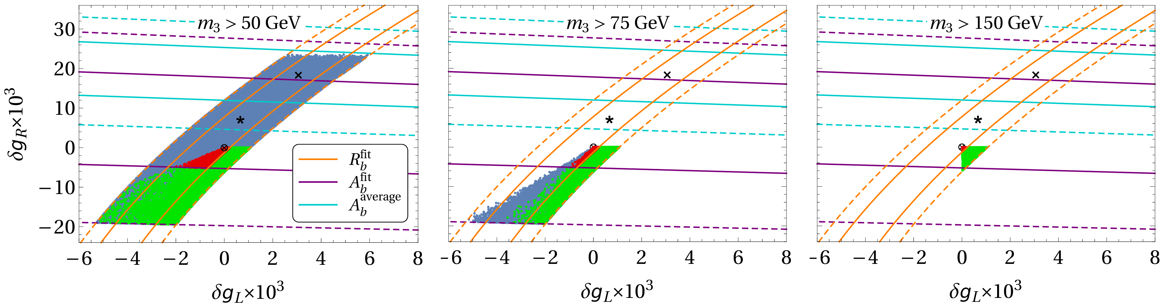
Figure 6: Scatter plot of values of $\delta g_{L}$ and $\delta g_{R}$ in the aligned 2HDM. A crossed circle marks the point $\delta g_{L}=\delta g_{R}=0$. A star marks the best-fit point of solution 1^fit, and a cross the best-fit point of solution 1^average. The orange lines mark the $1\sigma$ (full lines) and $2\sigma$ (dashed lines) boundaries of the region determined by the experimental value (10a); similarly, the violet lines correspond to the value (10b) and the light-blue lines to the value (11). Red points agree with the $1\sigma$ intervals (10); green points agree with the $2\sigma$, but not with the $1\sigma$, intervals (10); and blue points agree either with the $1\sigma$ or the $2\sigma$ intervals (10). Both the red and the green points satisfy the $1\sigma$ limits in equation (41), while the blue points comply with laxer conditions where $S$ can reach $2\sigma$ bounds and $T$ can reach $3\sigma$ bounds in equation (41). Note that some blue points are underneath either red or green points. Left panel: both new neutral scalars have masses above 50 GeV; middle panel: both new neutral scalars have masses above 75 GeV; right panel: both new neutral scalars have masses above 150 GeV.

One sees that, if one forces the 2HDM to comply with the $S$ and $T$-oblique parameter constraints (41), then the 2HDM cannot achieve a better agreement with solution 1 for $g_{L}$ and $g_{R}$ than the SM; in particular, when one uses the $A_{b}$ value (11), the 2HDM cannot even reach the $2\sigma$ interval. Only when one allows both for a laxer $S$- and $T$-oblique parameters constraints and for a very low neutral-scalar mass $m_{3}\lesssim 60$ GeV are the central values of both solutions 1^fit and 1^average attainable. In the right panel of figure 6 one sees that, if both new neutral scalars of the 2HDM have masses larger than 150 GeV, then the fit to solution 1 is never better than in the SM case, even if one does not take into account the $S$ and $T$-parameter constraints.

In figure 7 we display the same points as in figure 6, now distinguishing the neutral-scalar contribution to $\delta g_{L}$ from the charged-scalar contribution to the same quantity.

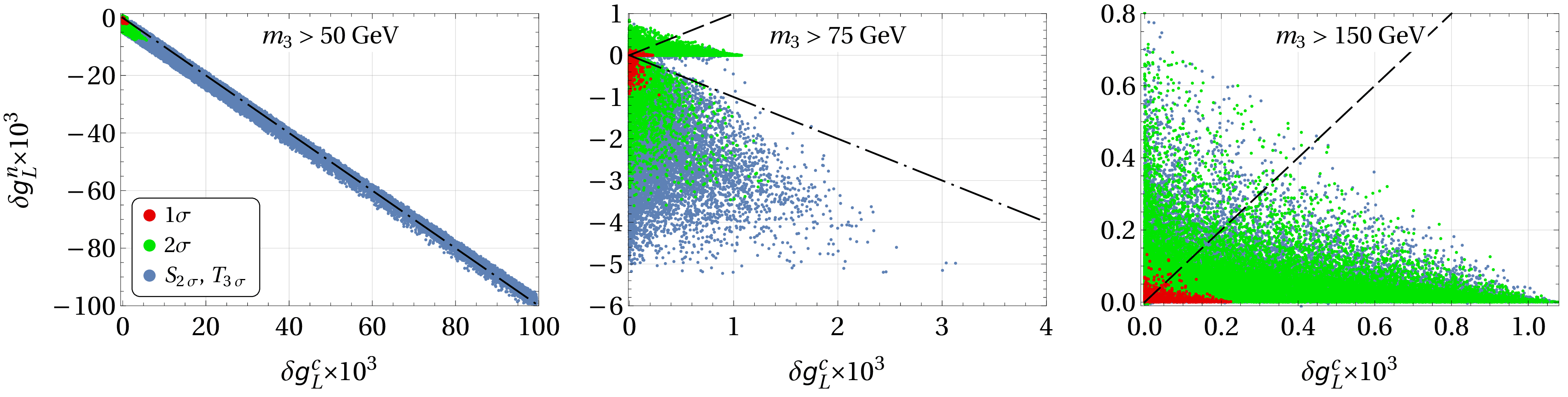
Figure 7: Scatter plot of $\delta g_{L}^{n}$ versus $\delta g_{L}^{c}$ in the aligned 2HDM. The displayed points and the colour code employed are the same as in figure 6. The dashed straight lines mark the condition $\delta g_{L}^{n}=\delta g_{L}^{c}$ and the dashed-dotted lines correspond to $\delta g_{L}^{n}=-\delta g_{L}^{c}$. Notice the vastly different scales in the three panels.

The same exercise is performed in figure 8 for the contributions to $\delta g_{R}$.

Figure 8: Scatter plot of $\delta g_{R}^{n}$ versus $\delta g_{R}^{c}$ in the aligned 2HDM. The displayed points and the colour code employed are the same as in figure 6. The dashed straight lines mark the condition $\delta g_{R}^{n}=\delta g_{R}^{c}$ and the dashed-dotted lines correspond to $\delta g_{R}^{n}=-\delta g_{R}^{c}$.

In the left panels of figures 7 and 8 one can see that the agreement of some blue points with solution 1^fit is obtained not just by using very light neutral scalars and laxer oblique parameters $S$ and $T$, but also through a fine-tuning where large neutral-scalar and charged-scalar contributions almost cancel each other. In the right panels of those figures one sees that, when both neutral scalars have masses above 150 GeV, the signs of the neutral-scalar and charged-scalar contributions are the same—this explains the agreement worse than in the SM observed in figure 6.

One also sees in figures 7 and 8 that the neutral-scalar contributions $\delta g_{L}^{n}$ and $\delta g_{R}^{n}$ are often comparable in size to, or even larger than, the charged-scalar contributions $\delta g_{L}^{c}$ and $\delta g_{R}^{c}$, respectively. Thus, the usual practice of taking into account just the charged-scalar contribution may lead to erroneous results.

One might hope the situation of disagreement with experiment to be milder in the 3HDM relative to the 2HDM, but one sees in figure 9 that this hardly happens.

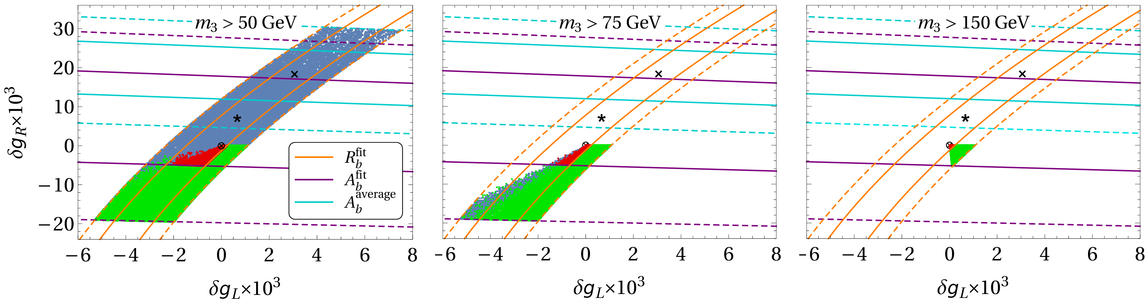
Figure 9: Scatter plot of values of $\delta g_{L}$ and $\delta g_{R}$ in the aligned 3HDM. All the conventions are the same as in figure 6.

The agreement of the 3HDM with experiment may be better than the one of the 2HDM, but only in the case where very light neutral scalars exist. We have checked that, just as in the 2HDM, the better agreement occurs through an extensive finetuning where $\delta g_{L}^{n}\approx-\delta g_{L}^{c}$ and $\delta g_{R}^{n}\approx-\delta g_{R}^{c}$.

In figures 6–9 we have tried, and failed, to make the fits of solution 1 in the 2HDM and in the 3HDM better than in the SM. Things are different with solution 2, which the $n$HDM models can easily reproduce—with some caveats. We remind the reader that in solution 2 the parameter $g_{L}$ is about the same as predicted by the SM, but the parameter $g_{R}$ has sign opposite to the one in the SM, viz. $g_{R}\approx-0.08$ in solution 2 while $g_{R}\approx+0.08$ in the SM. In the left panel of figure 10 and in figure 11 we see how the fit of solution 2 works out in the case of the 2HDM.

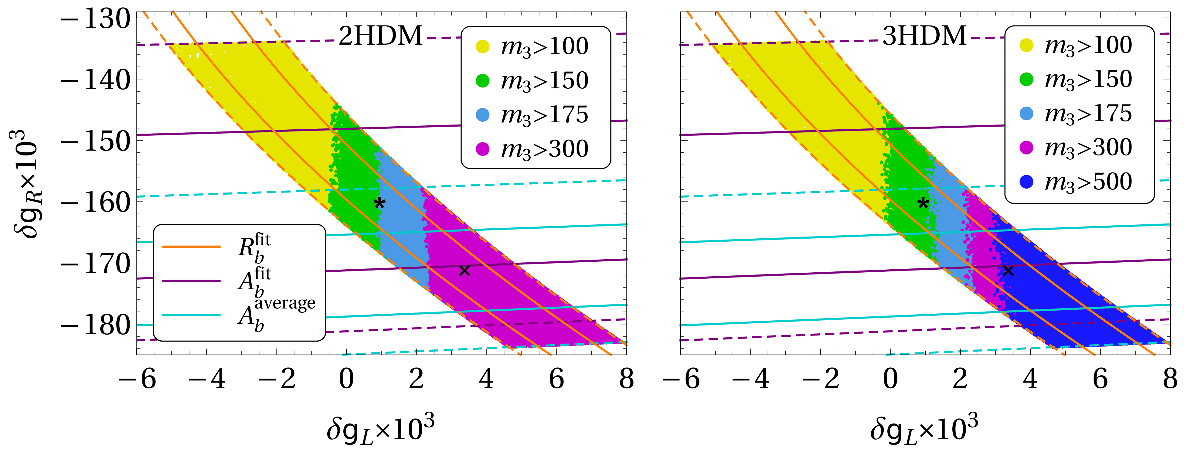
Figure 10: Scatter plot of values of $\delta g_{L}$ and $\delta g_{R}$ in the aligned 2HDM (left panel) and in the aligned 3HDM (right panel) that suit the solution 2 for $R_{b}$ and $A_{b}$. All the points depicted comply with the $S$ and $T$-oblique parameters constraint of equation (41). A star marks the best-fit point of solution 2^fit, and a cross the best-fit point of solution 2^average. The orange lines mark the $1\sigma$ (full lines) and $2\sigma$ (dashed lines) boundaries of the region determined by the experimental value (10a); similarly, the violet lines correspond to the value (10b) and the light-blue lines to the value (11). Blue points have new neutral scalars heavier than 500 GeV, pink points have them heavier than 300 GeV, light blue points have the lightest new neutral scalar in between 175 GeV and 300 GeV, green points have it in between 150 GeV and 175 GeV, and yellow points have it between 100 GeV and 150 GeV.

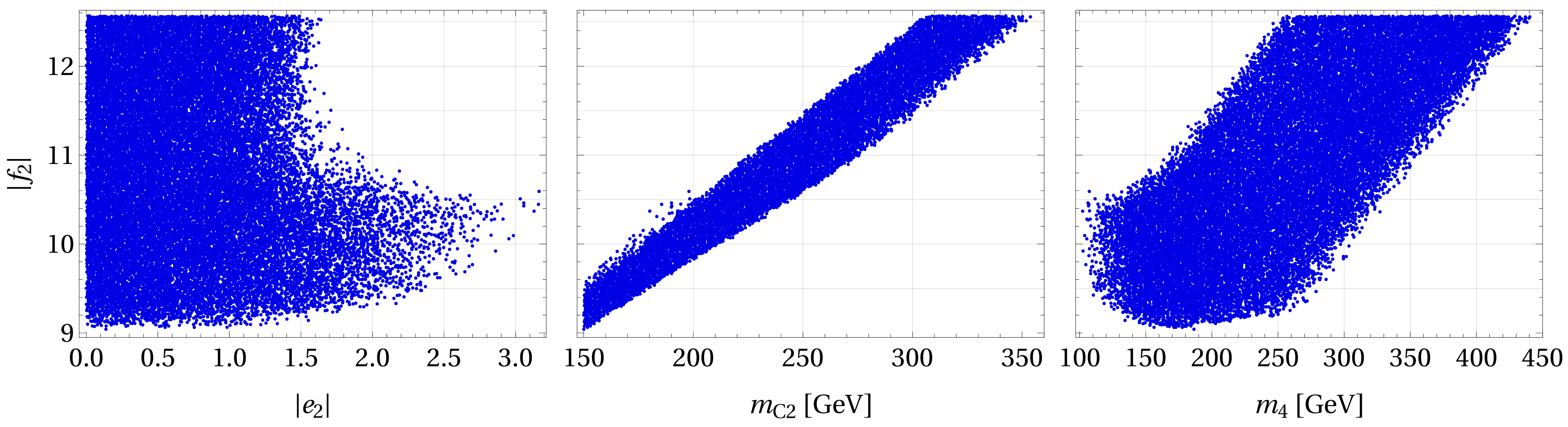
Figure 11: Scatter plot of 2HDM points that obey the $S$- and $T$-oblique parameters constraints, fit solution 2^average at the 1$\sigma$ level, and have $m_{3}>100$ GeV.

One sees that one can attain the 1$\sigma$ intervals and the best-fit points both of solution 2^fit and of solution 2^average, but this requires (1) the new scalars of the 2HDM to be lighter than 440 GeV, (2) the Yukawa coupling $f_{2}$ to be quite large, and (3) the Yukawa coupling $e_{2}$ to be relatively small, possibly even zero. In practice, the upper bound on the masses of the scalars originates in the upper bound that unitarity imposes on $f_{2}$, as seen in the middle panel of figure 11; we have taken (rather arbitrarily) that upper bound to be $\left|f_{2}\right|<4\pi\approx 12.5$. In the left panel of figure 11 one sees that $\left|f_{2}\right|$ must be larger than 9 anyway. It is also clear from figure 10 that, the lighter the new scalars are allowed to be, the easier it is to reproduce solution 2; moreover, it is easier to reproduce solution 2^average, viz. with the value (11) for $A_{b}$, than solution 2^fit, viz. with the value (10b) for $A_{b}$, because solution 2^average does not necessitate $m_{3}$ to be as low as solution 2^fit.

In the right panel of figure 10 and in figures 12 and 13 we illustrate the fitting of solution 2 in the 3HDM. Comparing the left and right panels of figure 10, we see that the 2HDM and the 3HDM give similar results, but in the 3HDM it is possible to reach solution 2^average with larger masses of the new scalars. Indeed, in the 3HDM the lightest neutral scalar $m_{3}$ may be as heavy as 620 GeV, while in the 2HDM $m_{3}<420$ GeV. Like in figure 11, in figures 12 and 13 we have used points that satisfy the $S$- and $T$-parameters $1\sigma$ bounds (41), that fall into the 1$\sigma$ intervals of $\delta g_{L}$ and $\delta g_{R}$ for solution 2^average, and that have $m_{3}>100$ GeV. In figure 12 we display the charged- and neutral-scalar contributions to $\delta g_{L}$ and $\delta g_{R}$.

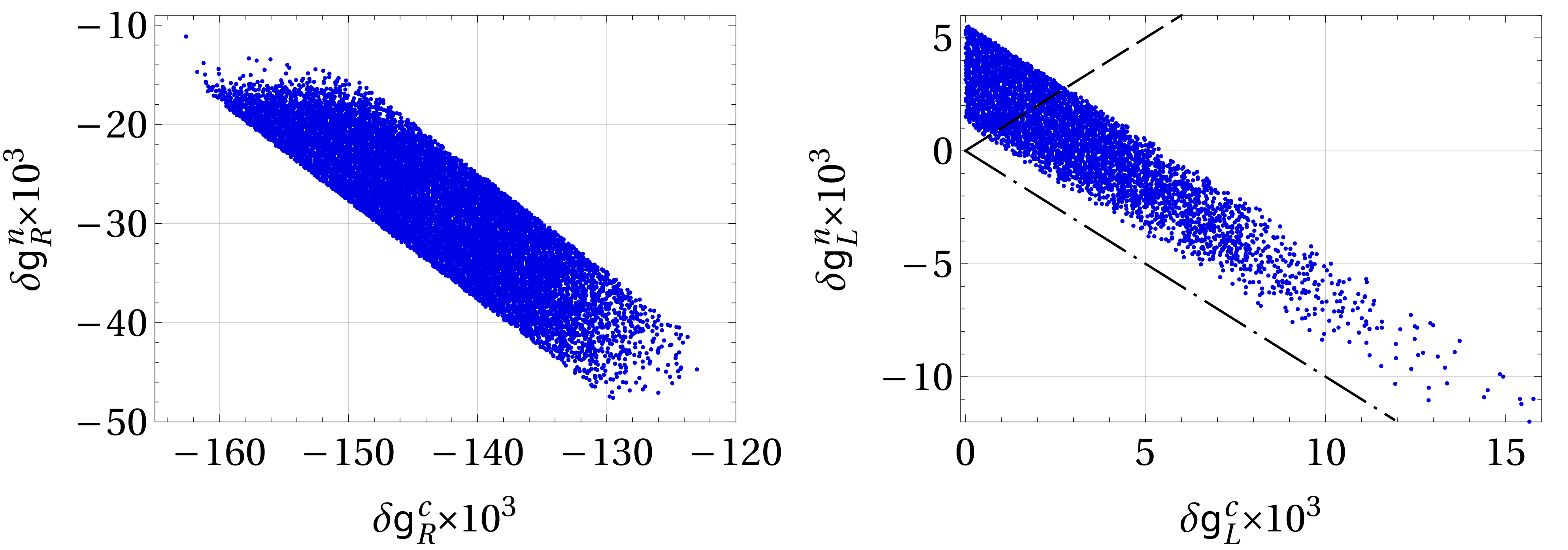
Figure 12: Scatter plot of 3HDM points that obey the $S$- and $T$-oblique parameters constraints, fit solution 2^average at the 1$\sigma$ level, and have $m_{3}>100$ GeV. Left panel: the neutral-scalar contribution to $\delta g_{R}$ versus the charged-scalar contribution to the same quantity. Right panel: the same for $\delta g_{L}$ instead of $\delta g_{R}$. In the right panel, the dashed line marks the condition $\delta g_{L}^{n}=\delta g_{L}^{c}$ and the dashed-dotted line corresponds to $\delta g_{L}^{n}=-\delta g_{L}^{c}$.

One sees that solution 2 may be considered a finetuning, with $\left|\delta g_{R}^{c}\right|\gg\left|\delta g_{R}^{n},\,\delta g_{L}^{c},\,\delta g_{L}^{n}\right|$. We stress once again that the neutral-scalar contributions are as instrumental as the charged-scalar ones in obtaining decent fits. In figure 13 we illustrate the moduli of the $f$ Yukawa couplings and their relationship to the masses of the scalars.

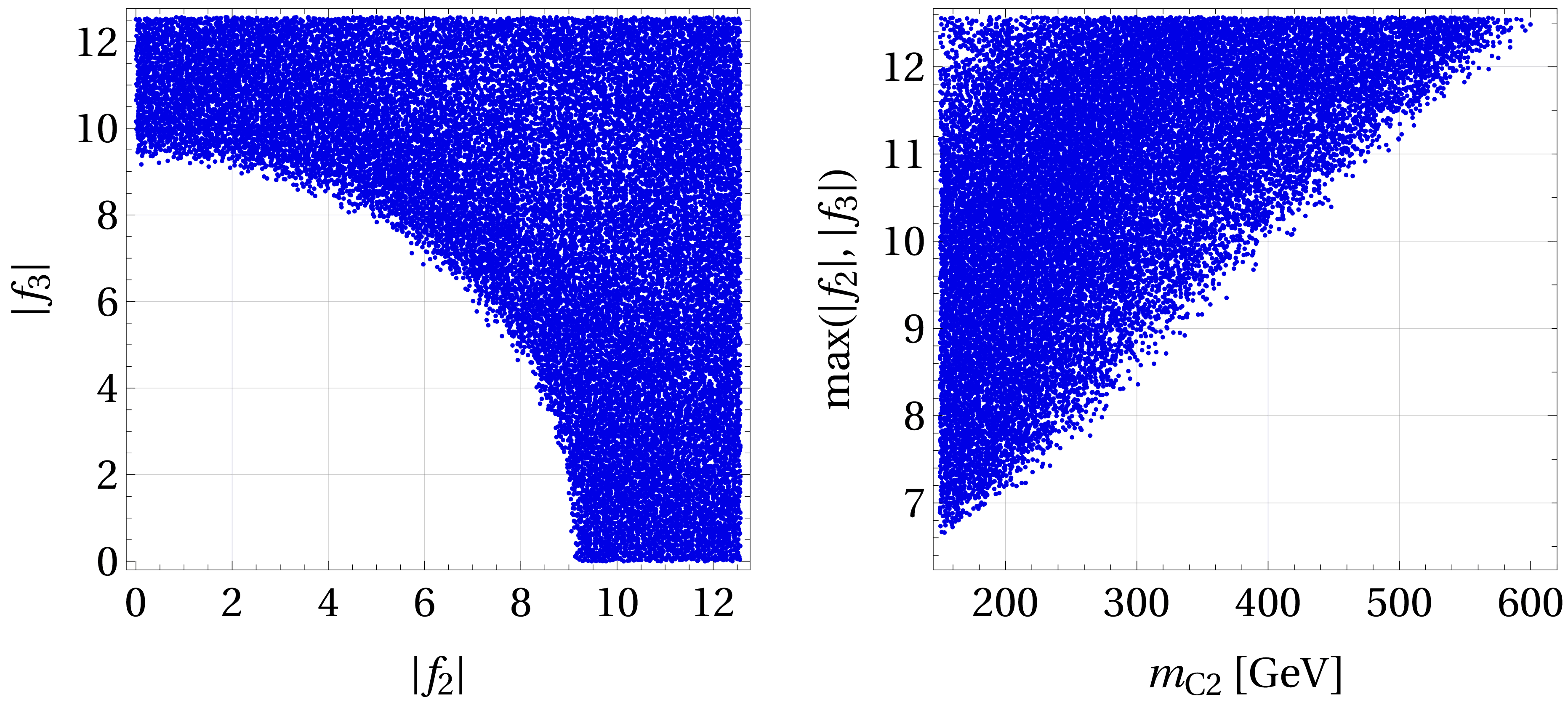
Figure 13: Scatter plot of 3HDM points that obey the $S$- and $T$-oblique parameters constraints, fit solution 2^average at the 1$\sigma$ level, and have $m_{3}>100$ GeV. Left panel: the modulus of the Yukawa coupling $f_{3}$ versus the modulus of $f_{2}$. Right panel: the largest of the two Yukawa couplings $f_{2}$ and $f_{3}$ versus the mass of the lightest charged scalar.

One sees that there is a bound $\sqrt{\left|f_{2}\right|^{2}+\left|f_{3}\right|^{2}}\gtrsim 9$, but each one of the Yukawa couplings $f_{2}$ and $f_{3}$ may separately vanish. One also observes that there is a simple straight-line correlation between the maximum possible value for the mass of the lightest charged scalar, $m_{C2}$, and the minimum possible value for the largest of the Yukawa couplings $f_{2}$ and $f_{3}$. It is worth pointing out that in the 3HDM, just as in the 2HDM, the masses $m_{3}$, $m_{4}$, and $m_{C2}$ must be low (because of the unitarity upper bound on the $f$ Yukawa couplings), but in the 3HDM the masses $m_{5}$, $m_{6}$, and $m_{C3}$ do not need to be low—they may be of order TeV.

6 Conclusions

The Standard Model (SM) has a slight problem in fitting the $Zb\bar{b}$ vertex, since it produces a $g_{R}$ smaller than what is needed to reproduce the fit (10); this discrepancy becomes larger when one uses for $A_{b}$ the value (11). In this paper we have found that this small problem can only worsen when one extends the SM through a $n$HDM. This is because the contributions of the new scalars usually produce a negative $\delta g_{R}$, i.e. they go in the wrong direction to alleviate the problem, aggravating it instead.

There is one possible escape from this conclusion if the extra neutral scalars of the $n$HDM are very light, i.e. lighter than the Fermi scale, because the contribution of the neutral scalars to $\delta g_{R}$ may in that case be positive and partially compensate for the inevitably negative contribution of the charged scalars. This is a contrived effort, though, both because it is experimentally difficult to accomodate very light neutral scalars and because, from the theoretical side, light neutral scalars together with heavy charged scalars easily lead to a much-too-large oblique parameter $T$.

In this paper we have considered the possibility that, in $n$HDM models, we might look instead at an alternative fit of the $Zb\bar{b}$ vertex, wherein $g_{R}$ has the opposite sign from the one predicted by the SM. This is what we have called “solution 2” in table 1. That solution necessitates a very large negative $\delta g_{R}$ (together with a small $\delta g_{L}$), that may seem like a finetuning, but is easy to obtain in a $n$HDM. This solution, though, also works only if the new scalars are relatively light and if at least one of the Yukawa couplings denoted $f_{k}$ in equation (16) is quite large, viz. larger than 9 or so.

Acknowledgements:

D.J. thanks the Lithuanian Academy of Sciences for financial support through projects DaFi2019 and DaFi2021. L.L. thanks the Portuguese Foundation for Science and Technology for support through CERN/FIS-PAR/0004/2019, CERN/FIS-PAR/0008/2019, PTDC/FIS-PAR/29436/2017, UIDB/00777/2020, and UIDP/00777/2020.

Appendix A Definition and measurements of $R_{b}$ and $A_{b}$

The experimental quantities $R_{b}$ and $A_{b}$ are defined for $e^{+}e^{-}$ collisions at the $Z^{0}$ peak, i.e. with $\sqrt{s}\approx m_{Z}$. Let the quark $q$ ($q=u,d,s,c,b$) couple to the $Z^{0}$ as

$$\mathcal{L}_{Zqq}=\frac{g}{c_{w}}\,Z_{\mu}\,\bar{q}\gamma^{\mu}\left(g_{Lq}P_{L}+g_{Rq}P_{R}\right)q.$$ (A1)

One has

$$g_{Lq}=\frac{1}{2}-\frac{2s_{w}^{2}}{3},\quad\quad g_{Rq}=-\frac{2s_{w}^{2}}{3}$$ (A2)

for $q=c$ and $q=u$, and

$$g_{Lq}=\frac{s_{w}^{2}}{3}-\frac{1}{2},\quad\quad g_{Rq}=\frac{s_{w}^{2}}{3}$$ (A3)

for $q=b$, $q=s$, and $q=d$. The probability that one produces a $q\bar{q}$ pair in an $e^{+}e^{-}$ collision at the $Z^{0}$ peak is, in the absence of QCD, QED, and mass corrections proportional to

$$s_{q}=2\left(g_{Lq}^{2}+g_{Rq}^{2}\right).$$ (A4)

One finds from equations (A2)–(A4) that

$$s_{c}+s_{u}+s_{s}+s_{d}=2-4s_{w}^{2}+\frac{40}{9}\,s_{w}^{4}\approx 1.32827.$$ (A5)

The experimental definition of $R_{b}$ is

$$R_{b}=\frac{\Gamma_{b\bar{b}}}{\Gamma_{\mathrm{hadrons}}}$$ (A6)

in $e^{+}e^{-}$ collisions at the $Z^{0}$ peak; thus, $R_{b}$ is the fraction of the produced hadrons that contain a $b\bar{b}$ pair. Clearly, in the absence of QCD, QED, and mass corrections,

$$R_{b} = \frac{s_{b}}{s_{b}+s_{c}+s_{u}+s_{s}+s_{d}}$$ (A7a)

$$= \frac{9-12s_{w}^{2}+8s_{w}^{4}}{45-84s_{w}^{2}+88s_{w}^{4}}\approx 0.21937.$$ (A7b)

When one includes QCD, QED, and mass corrections equation (A7a) gets substituted by equation (7) and $R_{b}$ decreases from the value in equation (A7b) to the SM prediction [4] 0.21581. Similarly, $s_{c}+s_{u}+s_{s}+s_{d}$ becomes 1.3184 instead of 1.32827 as in equation (A5).

If the mass of the bottom quark was zero, equation (5) would read

$$A_{b}=\frac{g_{L}^{2}-g_{R}^{2}}{g_{L}^{2}+g_{R}^{2}}=\frac{9-12s_{w}^{2}}{9-12s_{w}^{2}+8s_{w}^{4}}\approx 0.94059$$ (A8)

at the tree level. The quantity $A_{b}$ was accessed at LEP 1 through the forward–backward asymmetry of the produced $b\bar{b}$ quark pairs,

$$A_{\mathrm{FB}}^{0,b}=\frac{3}{4}\,A_{e}A_{b},$$ (A9)

where $A_{e}$, that is

$$A_{e}=\frac{1-4s_{w}^{2}}{1-4s_{w}^{2}+8s_{w}^{4}}\approx 0.21065$$ (A10)

at the tree level, can be extracted from other experiments. Equation (A9) is the limit of

$$A^{P_{e},b}_{\mathrm{FB}}=\frac{3}{4}\,\frac{A_{e}+P_{e}}{1+A_{e}P_{e}}\,A_{b}$$ (A11)

when the polarization $P_{e}$ of the electron beam is zero. The SLD Collaboration has used polarized beams ($P_{e}=1$) and therefore it could directly access

$$\frac{3}{4}\,A_{b}=\frac{\sigma_{L\mathrm{F}}+\sigma_{R\mathrm{B}}-\sigma_{L\mathrm{B}}-\sigma_{R\mathrm{F}}}{\sigma_{L\mathrm{F}}+\sigma_{R\mathrm{B}}+\sigma_{L\mathrm{B}}+\sigma_{R\mathrm{F}}},$$ (A12)

where the subscripts $L$ and $R$ refer to the electron’s polarization and the subscripts F and B refer to the forward or backward direction of travel of the final-state bottom quarks.

The value of $A_{b}$ obtained from the SLD measurement is $A_{b}^{\mathrm{fit}}=0.923\pm 0.020$ and is $0.6\sigma$ below the SM value [1]. However, this good agreement only applies to the overall fit of many observables. Extracting $A_{b}$ from $A_{\mathrm{FB}}^{0,b}$ when $A_{e}=0.1501\pm 0.0016$ leads to $A_{b}=0.885\pm 0.0017$, which is $2.9\sigma$ below the SM prediction. The combined value $A_{b}=0.901\pm 0.013$ deviates from the SM value by $2.6\sigma$. These discrepancies in $A_{b}$ could be an evidence of New Physics, but they could also be due to a statistical fluctuation or another experimental effect in one of asymmetries; more precise experiments are needed.

A direct measurement of the $Zb\bar{b}$ couplings at the LHC is challenging because of the large backgrounds in the detection of a $Z^{0}$ decaying into a bottom quark–antiquark pair. A recent study [6] has proposed a novel method to probe the anomalous $Zb\bar{b}$ couplings through the measurement of the cross section of the associated production $gg\to Zh$ at the High Luminosity LHC.

Lepton colliders of the next generation, vg. the CEPC, ILC, or FCC-ee offer great opportunities for further studies of the $Zb\bar{b}$ vertex, because they could collect a large amount of data around the $Z^{0}$ pole. In the analysis [25] there is a list of the observables that are most important for improving the constraints on the $Zb\bar{b}$ coupling, and of the expected precision reach of those three proposed future $e^{+}e^{-}$ colliders. These estimates, for the observables directly related to the $Zb\bar{b}$ coupling, are summarized in table 2.

Observable	Current	Precision
	measurement	Current	CEPC	ILC	FCC-ee
$R_{b}$	0.21629	0.00066	0.00017	0.00014	0.00006
		(0.00050)	(0.00016)		(0.00006)
$A_{\mathrm{FB}}^{0,b}$	0.0996	0.0016	0.00015
		(0.0007)	(0.00014)
$A_{b}$	0.923	0.020		0.001	0.00021
					(0.00015)
# of $Z^{0}$s	$\sim 2\times 10^{7}$		$\sim 2\times 10^{9}$	$\sim 10^{9}$	$\sim 10^{12}$

Table 2: The estimated precision reach for $Zb\bar{b}$ observables at future $e^{+}e^{-}$ colliders according to ref. [25]. The present result for each observable is shown in the second column. The third column shows the $\sigma$ of the present measurements at LEP and SLC, respectively, while the other columns show the estimates of the precision reach for the future colliders. In each entry, the number in the top line shows the total uncertainty and the number (in parenthesis) in the bottom line shows the systematic uncertainty. The last row shows the expected number of $Z^{0}$ events that will be collected.

We see that, with an increase of precision of more than one order of magnitude, a future collider has the potential to solve the $A_{\mathrm{FB}}^{0,b}$ discrepancy found at LEP. If its results are SM-like, a future lepton collider can provide strong constraints on models beyond the SM; if the $A_{\mathrm{FB}}^{0,b}$ discrepancy found at LEP does come from New Physics, then any of the three next-generation $e^{+}e^{-}$ colliders will be able to rule out the SM with more than $5\sigma$ significance [25].

Appendix B General formula for the neutral-scalar contribution

According to ref. [15], the contributions to $\delta g_{L}$ and $\delta g_{R}$ of loops with internal lines of neutral scalars and bottom quarks are the sums of three types of Feynman diagrams. Thus,

$$\delta g_{L}^{n}=\delta g_{L}^{n}(a)+\delta g_{L}^{n}(b)+\delta g_{L}^{n}(c),\quad\delta g_{R}^{n}=\delta g_{R}^{n}(a)+\delta g_{R}^{n}(b)+\delta g_{R}^{n}(c).$$ (B1)

Equations (24), (42), and (46) of ref. [15] inform us that

$$\delta g_{L}^{n}(a) = \frac{-i}{32\pi^{2}}\sum_{l,l^{\prime}=1}^{2n}\mathcal{A}_{ll^{\prime}}\left(\mathcal{V}^{T}F\right)_{l}\left(\mathcal{V}^{\dagger}F^{\ast}\right)_{l^{\prime}}\,C_{00}\left(0,\,m_{Z}^{2},\,0,\,0,\,m_{l^{\prime}}^{2},\,m_{l}^{2}\right),$$ (B2a)

$$\delta g_{R}^{n}(a) = \frac{-i}{32\pi^{2}}\sum_{l,l^{\prime}=1}^{2n}\mathcal{A}_{ll^{\prime}}\left(\mathcal{V}^{\dagger}F^{\ast}\right)_{l}\left(\mathcal{V}^{T}F\right)_{l^{\prime}}\,C_{00}\left(0,\,m_{Z}^{2},\,0,\,0,\,m_{l^{\prime}}^{2},\,m_{l}^{2}\right),$$ (B2b)

where $\mathcal{A}$ is the matrix defined in equation (15), and

$$F=\left(\begin{array}[]{c}\left.\sqrt{2}m_{b}\right/\!v\\[1.42262pt] f_{2}\\ \vdots\\ f_{n}\end{array}\right)$$ (B3)

is a vector formed by Yukawa coupling constants. Now,

$$C_{00}\left(0,\,m_{Z}^{2},\,0,\,0,\,m_{l^{\prime}}^{2},\,m_{l}^{2}\right)=C_{00}\left(0,\,m_{Z}^{2},\,0,\,0,\,m_{l}^{2},\,m_{l^{\prime}}^{2}\right),$$ (B4)

while $\mathcal{A}_{ll^{\prime}}=-\mathcal{A}_{l^{\prime}l}$. Therefore, equations (B2) may be rewritten

$$\delta g_{L}^{n}(a) = \frac{1}{16\pi^{2}}\sum_{l=2}^{2n-1}\sum_{l^{\prime}=l+1}^{2n}\mathcal{A}_{ll^{\prime}}\,\mathrm{Im}\left[\left(\mathcal{V}^{T}F\right)_{l}\left(\mathcal{V}^{\dagger}F^{\ast}\right)_{l^{\prime}}\right]C_{00}\left(0,\,m_{Z}^{2},\,0,\,0,\,m_{l^{\prime}}^{2},\,m_{l}^{2}\right),\hskip 8.53581pt$$ (B5a)

$$\delta g_{R}^{n}(a) = -\delta g_{L}^{n}(a),$$ (B5b)

where we have dropped from the sum over the scalars the Standard-Model contribution proportional to $\mathcal{A}_{12}$.

According to equations (2), (25), and (26) of ref. [15],

$$\delta g_{L}^{n}(b)+\delta g_{L}^{n}(c) = \frac{1}{16\pi^{2}}\sum_{l=2}^{2n}\left|\left(\mathcal{V}^{T}F\right)_{l}\right|^{2}\theta\left(m_{l}^{2}\right),$$ (B6a)

$$\delta g_{R}^{n}(b)+\delta g_{R}^{n}(c) = \frac{1}{16\pi^{2}}\sum_{l=2}^{2n}\left|\left(\mathcal{V}^{T}F\right)_{l}\right|^{2}\lambda\left(m_{l}^{2}\right),$$ (B6b)

where

$$\theta\left(m_{l}^{2}\right) := \frac{s_{w}^{2}}{6}\left[2\,C_{00}\left(0,\,m_{Z}^{2},\,0,\,m_{l}^{2},\,0,\,0\right)-\frac{1}{2}\right.$$ (B7a)

$$\left.-m_{Z}^{2}\,C_{12}\left(0,\,m_{Z}^{2},\,0,\,m_{l}^{2},\,0,\,0\right)\vphantom{\frac{1}{2}}\right]+\left(\frac{s_{w}^{2}}{6}-\frac{1}{4}\right)B_{1}\left(0,\,0,\,m_{l}^{2}\right),$$

$$\lambda\left(m_{l}^{2}\right) := \left(\frac{s_{w}^{2}}{6}-\frac{1}{4}\right)\left[2\,C_{00}\left(0,\,m_{Z}^{2},\,0,\,m_{l}^{2},\,0,\,0\right)-\frac{1}{2}\right.$$ (B7b)

$$\left.-m_{Z}^{2}\,C_{12}\left(0,\,m_{Z}^{2},\,0,\,m_{l}^{2},\,0,\,0\right)\vphantom{\frac{1}{2}}\right]+\frac{s_{w}^{2}}{6}\,B_{1}\left(0,\,0,\,m_{l}^{2}\right).$$

We now write

$$\mathcal{V}=\mathcal{R}+i\mathcal{I},$$ (B8)

where the $n\times 2n$ matrices $\mathcal{R}$ and $\mathcal{I}$ are real and satisfy

$$\mathcal{R}\mathcal{R}^{T}=\mathcal{I}\mathcal{I}^{T}=\mathbbm{1}_{n_{d}\times n_{d}},\quad\mathcal{R}\mathcal{I}^{T}=\mathcal{I}\mathcal{R}^{T}=0_{n_{d}\times n_{d}},$$ (B9)

cf. equation (14). From equation (B8),

$$\mathcal{A}:=\mathrm{Im}\left(\mathcal{V}^{\dagger}\mathcal{V}\right)=\mathcal{R}^{T}\mathcal{I}-\mathcal{I}^{T}\mathcal{R}.$$ (B10)

It follows that

$$\sum_{l^{\prime}=1}^{2n}\mathcal{A}_{ll^{\prime}}\left(\mathcal{V}^{\dagger}F^{\ast}\right)_{l^{\prime}}=-i\left(\mathcal{V}^{\dagger}F^{\ast}\right)_{l},\quad\sum_{l=1}^{2n}\left(\mathcal{V}^{T}F\right)_{l}\mathcal{A}_{ll^{\prime}}=-i\left(\mathcal{V}^{T}F\right)_{l^{\prime}}.$$ (B11)

Therefore, from equations (B6),

$$\delta g_{L}^{n}(b)+\delta g_{L}^{n}(c) = \frac{1}{32\pi^{2}}\left[\sum_{l=2}^{2n}\left(\mathcal{V}^{T}F\right)_{l}\left(\mathcal{V}^{\dagger}F^{\ast}\right)_{l}\theta\left(m_{l}^{2}\right)\right.$$ (B12b)

$$\left.+\sum_{l^{\prime}=2}^{2n}\left(\mathcal{V}^{T}F\right)_{l^{\prime}}\left(\mathcal{V}^{\dagger}F^{\ast}\right)_{l^{\prime}}\theta\left(m_{l^{\prime}}^{2}\right)\right]$$

$$= \frac{1}{32\pi^{2}}\left\{\sum_{l=2}^{2n}\left(\mathcal{V}^{T}F\right)_{l}\left[i\sum_{l^{\prime}=1}^{2n}\mathcal{A}_{ll^{\prime}}\left(\mathcal{V}^{\dagger}F^{\ast}\right)_{l^{\prime}}\right]\theta\left(m_{l}^{2}\right)\right.$$

$$\left.+\sum_{l^{\prime}=2}^{2n}\left[i\sum_{l=1}^{2n}\left(\mathcal{V}^{T}F\right)_{l}\mathcal{A}_{ll^{\prime}}\right]\left(\mathcal{V}^{\dagger}F^{\ast}\right)_{l^{\prime}}\theta\left(m_{l^{\prime}}^{2}\right)\right\}$$

$$= \frac{i}{32\pi^{2}}\sum_{l,l^{\prime}=1}^{2n}\left(\mathcal{V}^{T}F\right)_{l}\mathcal{A}_{ll^{\prime}}\left(\mathcal{V}^{\dagger}F^{\ast}\right)_{l^{\prime}}\left[\theta\left(m_{l}^{2}\right)+\theta\left(m_{l^{\prime}}^{2}\right)\right],$$ (B12c)

$$\delta g_{R}^{n}(b)+\delta g_{R}^{n}(c) = \frac{i}{32\pi^{2}}\sum_{l,l^{\prime}=1}^{2n}\left(\mathcal{V}^{T}F\right)_{l}\mathcal{A}_{ll^{\prime}}\left(\mathcal{V}^{\dagger}F^{\ast}\right)_{l^{\prime}}\left[\lambda\left(m_{l}^{2}\right)+\lambda\left(m_{l^{\prime}}^{2}\right)\right].$$ (B12d)

Thus, from equations (B1) and (B2),

$$\delta g_{L}^{n} = \frac{-i}{32\pi^{2}}\sum_{l,l^{\prime}=1}^{2n}\mathcal{A}_{ll^{\prime}}\left(\mathcal{V}^{T}F\right)_{l}\left(\mathcal{V}^{\dagger}F^{\ast}\right)_{l^{\prime}}\left[C_{00}\left(0,\,m_{Z}^{2},\,0,\,0,\,m_{l^{\prime}}^{2},\,m_{l}^{2}\right)\right.$$ (B13a)

$$\left.-\theta\left(m_{l}^{2}\right)-\theta\left(m_{l^{\prime}}^{2}\right)\right],$$

$$\delta g_{R}^{n} = \frac{-i}{32\pi^{2}}\sum_{l,l^{\prime}=1}^{2n}\mathcal{A}_{ll^{\prime}}\left(\mathcal{V}^{T}F\right)_{l}\left(\mathcal{V}^{\dagger}F^{\ast}\right)_{l^{\prime}}\left[-C_{00}\left(0,\,m_{Z}^{2},\,0,\,0,\,m_{l^{\prime}}^{2},\,m_{l}^{2}\right)\right.$$ (B13b)

$$\left.-\lambda\left(m_{l}^{2}\right)-\lambda\left(m_{l^{\prime}}^{2}\right)\right].$$

We define the functions

$$h_{L}\left(m_{l^{\prime}}^{2},\,m_{l}^{2}\right) := -C_{00}\left(0,\,m_{Z}^{2},\,0,\,0,\,m_{l^{\prime}}^{2},\,m_{l}^{2}\right)+\theta\left(m_{l^{\prime}}^{2}\right)+\theta\left(m_{l}^{2}\right),$$ (B14a)

$$h_{R}\left(m_{l^{\prime}}^{2},\,m_{l}^{2}\right) := C_{00}\left(0,\,m_{Z}^{2},\,0,\,0,\,m_{l^{\prime}}^{2},\,m_{l}^{2}\right)+\lambda\left(m_{l^{\prime}}^{2}\right)+\lambda\left(m_{l}^{2}\right).$$ (B14b)

These functions are symmetric under the interchange of their two arguments:

$$h_{L}\left(m_{l^{\prime}}^{2},\,m_{l}^{2}\right)=h_{L}\left(m_{l}^{2},\,m_{l^{\prime}}^{2}\right),\quad h_{R}\left(m_{l^{\prime}}^{2},\,m_{l}^{2}\right)=h_{R}\left(m_{l}^{2},\,m_{l^{\prime}}^{2}\right).$$ (B15)

Moreover, by utilizing equations (21) of ref. [15] it is easy to show that, although the functions $\theta\left(m_{l}^{2}\right)$, $\lambda\left(m_{l}^{2}\right)$, and $C_{00}\left(0,\,m_{Z}^{2},\,0,\,0,\,m_{l^{\prime}}^{2},\,m_{l}^{2}\right)$ contain divergences, the functions $h_{L}\left(m_{l^{\prime}}^{2},\,m_{l}^{2}\right)$ and $h_{R}\left(m_{l^{\prime}}^{2},\,m_{l}^{2}\right)$ do not. From equation (B13) we obtain

$$\delta g_{L}^{n} = \frac{1}{16\pi^{2}}\sum_{l=2}^{2n-1}\sum_{l^{\prime}=l+1}^{2n}\mathcal{A}_{ll^{\prime}}\,\mathrm{Im}\left[\left(\mathcal{V}^{\dagger}F^{\ast}\right)_{l}\left(\mathcal{V}^{T}F\right)_{l^{\prime}}\right]h_{L}\left(m_{l^{\prime}}^{2},\,m_{l}^{2}\right),$$ (B16a)

$$\delta g_{R}^{n} = \delta g_{L}^{n}\left[h_{L}\left(m_{l^{\prime}}^{2},\,m_{l}^{2}\right)\to h_{R}\left(m_{l^{\prime}}^{2},\,m_{l}^{2}\right)\right].$$ (B16b)

Thus, the functions $h_{L}$ and $h_{R}$ are crucial in the computation of the neutral-scalar contributions to $\delta g_{L}$ and $\delta g_{R}$, respectively. Those functions were not explicitly defined in ref. [15], even though they were utilized in that paper.

References

• [1] Particle Data Group collaboration, Prog. Theor. Exp. Phys. 2020 (2020) 083C01.
• [2] J. Field, Mod. Phys. Lett. A 13 (1998) 1937.
• [3] H. E. Haber and H. E. Logan, Phys. Rev. D 62 (2000) 015011.
• [4] J. Erler and A. Freitas, “Electroweak model and constraints on new physics,” in ref. [1], pp. 180 ff.
• [5] D. Choudhury, T. M. P. Tait, and C. E. M. Wagner, Phys. Rev. D 65 (2002) 053002.
• [6] B. Yan and C.-P. Yuan, arXiv:2101.06261 [hep-ph].
• [7] G. C. Branco, P. M. Ferreira, L. Lavoura, M. N. Rebelo, M. Sher, and J. P. Silva, Phys. Rept. 516 (2012) 1.
• [8] A. Pich and P. Tuzón, Phys. Rev. D 80 (2009) 091702.
• [9] A. Pilaftsis, Phys. Rev. D 93 (2016) 075012.
• [10] H. E. Logan, S. Moretti, D. Rojas-Ciofalo, and M. Song, arXiv:2012.08846 [hep-ph].
• [11] V. Keus, S. F. King, and S. Moretti, J. High Energ. Phys. 01 (2014) 052.
• [12] I. P. Ivanov and E. Vdovin, Eur. Phys. J. C 73 (2013) 2309.
• [13] D. Das and I. Saha, Phys. Rev. D 100 (2019) 035021.
• [14] M. P. Bento, H. E. Haber, J. C. Romão, and J. P. Silva, J. High Energ. Phys. 11 (2017) 095.
• [15] D. Fontes, L. Lavoura, J. C. Romão, and J. P. Silva, Nucl. Phys. B 958 (2020) 115131.
• [16] A. Denner, S. Dittmaier, and L. Hofer, Comput. Phys. Commun. 212 (2017) 220.
• [17] H. H. Patel, Comput. Phys. Commun. 197 (2015) 276.
• [18] G. C. Branco, P. M. Ferreira, L. Lavoura, M. N. Rebelo, M. Sher, and J. P. Silva. Phys. Rept. 516 (2012) 1.
• [19] A. Barroso, P. M. Ferreira, I. P. Ivanov, R. Santos, and J. P. Silva, Eur. Phys. J. C 73 (2013) 2537;
I. P. Ivanov, Phys. Rev. D 75 (2007) 035001 [erratum 76 (2007) 039902];
I. P. Ivanov, Phys. Rev. D 77 (2008) 015017;
I. P. Ivanov and J. P. Silva, Phys. Rev. D 92 (2015) 055017.
• [20] M. E. Peskin and T. Takeuchi, Phys. Rev. Lett. 65 (1990) 964;
G. Altarelli and R. Barbieri, Phys. Lett. B 253 (1991) 161;
M. E. Peskin and T. Takeuchi, Phys. Rev. D 46 (1992) 381;
G. Altarelli, R. Barbieri, and S. Jadach, Nucl. Phys. B 369 (1992) 3 [erratum 376 (1992) 444].
• [21] W. Grimus, L. Lavoura, O. M. Ogreid, and P. Osland, Nucl. Phys. B 801 (2008) 81.
• [22] W. Grimus, L. Lavoura, O. M. Ogreid, and P. Osland, J. Phys. G: Nucl. Part. Phys. 35 (2008) 075001.
• [23] P. M. Ferreira, I. P. Ivanov, E. Jiménez, R. Pasechnik, and H. Serôdio, J. High Energy Phys. 01 (2018) 065.
• [24] B. Batell, S. Gori, and L.-T. Wang, J. High Energ. Phys. 01 (2013) 139.
• [25] S. Gori, J. Gu, and L. T. Wang, J. High Energ. Phys. 04 (2016) 062.
• [26] M. Misiak et al., Phys. Rev. Lett. 114 (2015) 221801.
• [27] A. G. Akeroyd, S. Moretti, K. Yagyu, and E. Yildirim, Int. J. Mod. Phys. A 32 (2017) 1750145.
• [28] V. Khachatryan et al. (CMS Collaboration), j. High energ. Phys. 11 (2015) 018.
• [29] A. Arbey, F. Mahmoudi, O. Stal, and T. Stefaniak, Eur. Phys. J. C 78 (2018) 182.
• [30] D. Chowdhury and O. Eberhardt, J. High Energ. Phys. 05 (2018) 161.
• [31] O. Eberhardt, A. P. Martínez, and A. Pich, J. High Energ. Phys. 05 (2021) 005.