$\mathbb{Z}_{2}$ topological order and first-order quantum phase transitions
in systems with combinatorial gauge symmetry

Abstract

We study a generalization of the two-dimensional transverse-field Ising model, combining both ferromagnetic and antiferromagnetic two-body interactions, that hosts exact global and local $\mathbb{Z}_{2}$ gauge symmetries. Using exact diagonalization and stochastic series expansion quantum Monte Carlo methods, we confirm the existence of the topological phase in line with previous theoretical predictions. Our simulation results show that the transition between the confined topological phase and the deconfined paramagnetic phase is of first-order, in contrast to the conventional $\mathbb{Z}_{2}$ lattice gauge model in which the transition maps onto that of the standard Ising model and is continuous. We further generalize the model by replacing the transverse field on the gauge spins with a ferromagnetic $XX$ interaction while keeping the local gauge symmetry intact. We find that the $\mathbb{Z}_{2}$ topological phase remains stable, while the paramagnetic phase is replaced by a ferromagnetic phase. The topological–ferromagnetic quantum phase transition is also of first-order. For both models, we discuss the low-energy spinon and vison excitations of the topological phase and their avoided level crossings associated with the first-order quantum phase transitions.

I Introduction

Topological quantum states of matter are of central focus in modern condensed matter physics. One of the main features of strongly-interacting systems with gapped topological order is that they can present degenerate ground states. This degeneracy cannot be lifted by the action of local perturbations, and hence this property makes such systems perfect candidates for building stable (topological) qubits. Several theoretical models have been proposed to realize gapped topologically ordered states. For instance, the toric code Kitaev (2003) and dimer models on non-bipartite lattices Moessner and Sondhi (2001); Misguich et al. (2002) host quantum spin liquid (QSL) phases that possess $\mathbb{Z}_{2}$ topological order. In both these examples, the Hamiltonians contain multi-body interactions, making it a challenge to encounter materials realizing these phases or to realize them in artificial structures.

Attempts have been made to construct models with simpler interactions that can host gapped QSLs. A rare successful example is the cluster charging model of bosons on the kagome lattice Balents et al. (2002); Isakov et al. (2006, 2007), which has been shown theoretically and numerically to host a $\mathbb{Z}_{2}$ quantum spin liquid, in a system with only two-body interactions. However, these two-body interactions are of the $XXZ$ type, which are not easily implementable in, say, programmable quantum devices. Moreover, the $\mathbb{Z}_{2}$ gauge symmetry in this model is only emerging, i.e., it exists in the effective model derived in perturbation theory, but it is not an exact symmetry of the original Hamiltonian.

Recently, a construction for which the $\mathbb{Z}_{2}$ gauge symmetry is exact was proposed on a variant of the transverse field Ising model (TFIM), utilizing only simple two-body ferromagnetic and antiferromagnetic $ZZ$ interactions Chamon et al. (2020). Monomial (matrix) transformations that correspond to combinations of spin flips and permutations play a central role in the construction, thus dubbed combinatorial gauge symmetry. Because the construction utilizes only $ZZ$ interactions (of both signs) and a transverse field, the model can be easily implemented, for example, with current Noisy Intermediate-Scale Quantum (NISQ) technology using flux-based superconducting qubits, or other types of quantum computer architectures that provide similar interactions on qubits. The model has already been successfully implemented on a D-wave quantum device in a recent experiment Zhou et al. (2020).

In this paper, we present a quantitative and detailed study of the combinatorial $\mathbb{Z}_{2}$ gauge model originally proposed in Ref. Chamon et al., 2020. Two different types of quantum fluctuations are introduced while preserving the gauge symmetry: a transverse field acting on the gauge spins and a $XX$ ferromagnetic interaction between the gauge spins, respectively. In both cases, we observe the existence of a $\mathbb{Z}_{2}$ topological state separated by a first-order transition from another phase—a paramagnet in the first model and a ferromagnet in the second

The structure of the paper is as follows. First, in Sec. II we give a brief introduction to the model with combinatorial $\mathbb{Z}_{2}$ gauge symmetry. The model realizes the $\mathbb{Z}_{2}$ gauge symmetry through monomial transformations and effectively realizes the 4-body interaction term as the star term in the classical version of the toric code. We further introduce two types of quantum fluctuations by applying either a transverse field on the gauge spins (model-X) or a $XX$ ferromagnetic interaction between the gauge spins (model-XX), both of which respect the gauge symmetry. In Secs. III and IV, we provide numerical results on both models obtained from quantum Monte-Carlo (QMC) simulations with the Stochastic Series Expansion (SSE) method as well as exact diagonalization (ED). In both cases, we find that the system exhibits a $\mathbb{Z}_{2}$ topologically ordered phase separated by a first-order transition from either a paramagnetic phase (model-X) or a ferromagnetic phase (model-XX). We summarize our main results and discuss the remaining open questions and future prospects in Sec. V.

Figure 1: (a) The arrangement of two species of Ising spins on a square lattice. Gauge spins (green squares) reside on the links and four matter spins (orange dots) occupy each site of the square lattice. (b) The vertex unit and the interactions between spins. The interactions between gauge-matter spins within a single unit are defined by the Hadamard matrix $\mathbf{W}$ in Eq. (3). For clarity, the couplings are depicted on a deformed cell in panel (c), where the ferromagnetic and antiferromagnetic couplings are shown as thin blue lines and bold red lines, respectively.

II Spin models with combinatorial gauge symmetry

We consider two models in our studies starting from a baseline model that contains $ZZ$ interactions between the spins with both ferromagnetic and antiferromagnetic couplings arranged in a pattern such that the combinatorial gauge symmetry is realized.

On top of the baseline model, additional kinetic terms are introduced to give the system quantum dynamics. Here we consider two different types of kinetic terms. The first one is a transverse field on the gauge spins in what we call model-X; the second one is a ferromagnetic XX-type ($\sigma^{x}\sigma^{x}$) coupling between the gauge spins, which defines model-XX. In this section we start by describing the details of the baseline model and how the combinatorial gauge symmetry is realized. We then discuss the models with the two different kinetic terms.

II.1 Baseline model with combinatorial gauge symmetry

In the baseline model $S=1/2$ spins reside on both the sites and the links of a square lattice, as shown in Fig. 1(a). For each star (or vertex) $s$ of the lattice, we place four “matter” spins $\mu$ (the orange dots inside the circles representing the lattice sites) and four “gauge” spins $\sigma$ (green square) on the links of the star. One such star with its total of eight spins is depicted in Fig. 1(b) along with a labeling scheme. The Hamiltonian of the system is written as

$$H=\sum_{s}H_{s}+H^{\sigma}_{\rm kin}\;,$$ (1)

where $H^{\sigma}_{\rm kin}$ is the kinetic term involving only the $\sigma^{x}$ component of the gauge spins (on all links), and at each star $s$ we define a local Hamiltonian on its eight spins

$$H_{s}=J\sum_{a\in s}\left(\sum_{j\in s}W_{aj}\sigma^{z}_{j}\right)\mu^{z}_{a}-\Gamma_{m}\sum_{a\in s}\mu^{x}_{a}\;.$$ (2)

Here the sums with $j$ and $a$ indices include the four matter spins $\sigma^{z}_{j}$ and the four gauge spins $\mu^{z}_{a}$, respectively. Notice that $H_{s}$ contains a transverse field only on the matter spins. The $ZZ$ couplings between the gauge and matter spins have magnitude $J$ and signs controlled by the Hadamard matrix $W$,

$$\mathbf{W}=\begin{pmatrix}+1&-1&-1&-1\\ -1&+1&-1&-1\\ -1&-1&+1&-1\\ -1&-1&-1&+1\end{pmatrix}.$$ (3)

Fig. 1(c) depicts these signs; the interaction between a gauge spin and its nearest matter spin is antiferromagnetic (bold red line) while its interaction with the other 3 matter spins are ferromagnetic (thin blue line).

The Hamiltonian in Eq. (1) possesses combinatorial $\mathbb{Z}_{2}$ gauge symmetry if the $H_{s}$ terms are of the above form, and if only the $\sigma^{x}$ component of the gauge spins enters in $H^{\sigma}_{\rm kin}$. The transformations

$$\sigma^{z}_{i} \rightarrow\sum_{j}\mathbf{R}_{ij}\,\sigma_{j}^{z}$$ (4a)

$$\mu^{z}_{b} \rightarrow\sum_{a}\mu_{a}^{z}\,\mathbf{L}^{-1}_{ab}$$ (4b)

leave the spin commutation relations invariant if $\mathbf{L}$ and $\mathbf{R}$ are monomial matrices, i.e., generalized permutation matrices with a $\pm 1$ entry in each line or column in the case of the group $\mathbb{Z}_{2}$. The transformations correspond to combinations of rotations by 0 (+1 entry) or $\pi$ (-1 entry) around the $x$-axis, followed by a permutation of the indices.

A local gauge symmetry is generated by flipping gauge spins on closed loops around the elementary plaquettes, together with accompanying transformations on matter spins. Flipping the gauge spins around the loop corresponds to choosing $\mathbf{R}$ matrices for each $s$ traversed, with an even number of $-1$ entries associated with the links visited. For each such $\mathbf{R}$, there is a corresponding monomial matrix $\mathbf{L}=\mathbf{W}\,\mathbf{R}\,\mathbf{W}^{-1}$ Chamon et al. (2020). These pairs of monomial $\mathbf{R}$ and $\mathbf{L}$ matrices are such that $\mathbf{W}=\mathbf{L}^{-1}\,\mathbf{W}\,\mathbf{R}$, and thus the transformation in Eq. (4) leaves the $ZZ$ part of the Hamiltonian invariant. Moreover, since in $H_{s}$ the transverse field on the $\mu^{x}$ is the same on all $a\in s$, the permutation action of the monomial $\mathbf{L}$ also leaves these terms unchanged. Hence, $H_{s}$ is invariant under the monomial transformation with $\mathbf{L}$ and $\mathbf{R}$. Finally, since $\mathbf{R}$ is diagonal and only $\sigma^{x}$ enters in $H^{\sigma}_{\rm kin}$, this kinetic term is also invariant. For each such loop, we have a $\mathbb{Z}_{2}$ symmetry of the Hamiltonian in Eq. (1).

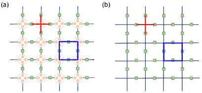
Figure 2: Connection between the model in our studies to the $\mathbb{Z}_{2}$ gauge theory. The red star in (a) represents the expanded 4-body interacting term that is equivalent to the star term $\prod\sigma^{z}$ of the $\mathbb{Z}_{2}$ gauge model in (b). The blue plaquette in (a) represents the local combinatorial gauge generator $G_{p}$ by analogy with the local gauge generator $G_{p}^{\mathrm{toric}}$ of the $\mathbb{Z}_{2}$ gauge model defined as $\prod\sigma^{x}$ of the 4 spins around a plaquette in (b).

This local $\mathbb{Z}_{2}$ gauge symmetry is exact for any value of the parameters in the Hamiltonian Eq. (1). We can obtain further intuition by connecting to the more familiar formulation of the $\mathbb{Z}_{2}$ gauge theory Wegner (1971); Kogut (1979) in certain limits. Consider the effective Hamiltonian for the $H_{s}$ terms when their energy scales are larger than those in $H^{\sigma}_{\rm kin}$; in this regime, one can diagonalize $H_{s}$ by fixing the $\sigma_{i}^{z}$ around the star and treating the problem as that of a paramagnet for the matter spins $\mu_{a}$. The result is an effective Hamiltonian for the lowest states that take the form of a four-spin interaction among the gauge spins:

$$H^{\rm eff}_{s}=-\gamma-\lambda\;\prod_{i\in s}\sigma_{i}^{z}\;,$$ (5a)

where the parameters $$\gamma \lambda$$ and are given by Chamon et al. (2020)

$$\gamma =\frac{1}{2}\left(\sqrt{\Gamma_{m}^{2}+16J^{2}}+3\Gamma_{m}+4\sqrt{\Gamma_{m}^{2}+4J^{2}}\right)$$ (5b)

$$\lambda =-\frac{1}{2}\left(\sqrt{\Gamma_{m}^{2}+16J^{2}}+3\Gamma_{m}-4\sqrt{\Gamma_{m}^{2}+4J^{2}}\right).$$ (5c)

Notice that the effective $H^{\rm eff}_{s}$ is, up to a constant shift, the same as the star term $A_{s}^{z}=\prod_{i\in s}\sigma_{i}^{z}$ that appears in the toric code Kitaev (2003) and the $\mathbb{Z}_{2}$ lattice gauge model Wegner (1971); Kogut (1979). We depict in Fig. 2(a) the star term in our model, juxtaposed to the star term represented in the toric and $\mathbb{Z}_{2}$ gauge models in Fig. 2(b) as the product of four spins on the red cross. The manifold of other states in our model, those beyond the effective term, are separated by a scale $\Gamma_{m}$. Thus, in the limit $\Gamma_{m}\to\infty$, higher energy sectors are projected out, and the system Hamiltonian asymptotically becomes the exact star term of the toric code.

In the conventional $\mathbb{Z}_{2}$ gauge transformation, the gauge operator $G_{p}^{\mathrm{toric}}=\prod_{i\in p}\sigma_{i}^{x}$ is built as a product of $\sigma_{i}^{x}$ spins along the smallest loops, shown as the blue square in Fig. 2(b)). In a system with Hamiltonian as in Eq. (1), which possesses combinatorial $\mathbb{Z}_{2}$ gauge symmetry, the exact local gauge transformation on a plaquette $p$ includes additional transformations corresponding to the action of an operator $\mathcal{L}_{s}^{\mu}$ on the matter spins of star $s$ as

$$\mathcal{L}_{s}^{\mu}\;\mu^{z}_{a}\;\left(\mathcal{L}_{s}^{\mu}\right)^{-1}=\sum_{b}\mu^{z}_{a}\;(\mathbf{L}^{-1})_{ba}\;,$$ (6)

which implements the flips and permutations associated to the monomial matrix $\mathbf{L}$. The plaquette term generating the combinatorial $\mathbb{Z}_{2}$ gauge symmetry is then defined as

$$G_{p}=\prod_{s\in p}\mathcal{L}_{s}^{\mu}\prod_{i\in p}\sigma_{i}^{x}.$$ (7)

In a system with linear size $L$ (total spins $N=L\times L\times 6$) and periodic boundary condition, one can find $M=2+(L^{2}-1)$ independent gauge operators $G_{p}$ that commute with the Hamiltonian Eq. (1). Within the $M$ operators, two of them, $G_{x}$ and $G_{y}$, are defined along non-contractible loops in the two spatial directions, and their quantum numbers uniquely characterize the topological ground state degeneracy. Therefore in the basis of these $G_{p}$ operators $G_{p}\ket{q}=q\ket{q}$ and the Hamiltonian can be block-diagonalized into $2^{M}$ blocks associated with unique quantum number sets $\mathbf{q}=(G_{x}=\pm 1,G_{y}=\pm 1;\pm 1,\pm 1,\dots)$ (See Appendix. A for details), where we list the quantum numbers of the non-contractible loops $G_{x}$ and $G_{y}$ first, and the remaining quantum numbers are associate to the other $M-2$ independent local gauge operators.

The discussion thus far is rather general, and, in particular, the combinatorial gauge symmetry is exact, provided that the kinetic term $H^{\sigma}_{\rm kin}$ involves only the $\sigma^{x}$ component. Below we shall discuss two different choices of $H^{\sigma}_{\rm kin}$.

II.2 Model with transverse field on the
gauge spins—model-X

A simple choice of kinetic term is to apply a transverse field on the gauge spins,

$$H^{\sigma}_{\rm kin}=-\Gamma_{g}\sum_{i}\sigma^{x}_{i}\;,$$ (8)

or, equivalently, the case with full Hamiltonian

$$H=J\sum_{a\in s}\left(\sum_{j\in s}W_{aj}\sigma^{z}_{j}\right)\mu^{z}_{a}-\Gamma_{m}\sum_{a\in s}\mu^{x}_{a}-\Gamma_{g}\sum_{i}\sigma^{x}_{i}\;.$$ (9)

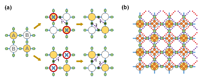
Figure 3: The second-order process generates the effective plaquette term in model-XX. The A-sublattice is marked in light yellow while the B-sublattice is indicated in white. (a) The processes that couple two stars in the A (top part) or B (bottom part) sublattice with an effective ferromagnetic interaction. (b) The arrangement of XX bonds (dashed lines) resulting in an effective TFIM on A and B sublattices. Different colors indicate bonds coupling sites in the A and B sublattices.

In the limit $\Gamma_{m}\gg J$, we can replace the first two terms by the star equivalent Eq. (5a). Therefore, Hamiltonian Eq. (9), which obeys the exact local combinatorial $\mathbb{Z}_{2}$ gauge symmetry, has the usual $\mathbb{Z}_{2}$ lattice gauge model as its low energy description:

$$H_{\mathbb{Z}_{2}}=-\lambda\sum_{s}\prod_{i\in s}\sigma^{z}_{i}-g\sum_{i}\sigma^{x}_{i},$$ (10)

with $g=\Gamma_{g}$ and $\lambda$ given by Eq. (5c). The $\mathbb{Z}_{2}$ lattice gauge model has been well studied and shown to host $\mathbb{Z}_{2}$ topological order for $g<g_{c}$, and undergo a deconfinement–confinement transition at $g=g_{c}$ that leads to a paramagnetic phase for $g>g_{c}$. The critical point is $g_{c}\approx 0.3285\lambda$ from the exact mapping to the dual 2D Ising model Rieger and Kawashima (1999); du Croo de Jongh and van Leeuwen (1998); Liu et al. (2013); Fradkin (2013). We expect similar phases to appear in the full Hamiltonian Eq (9) as the uniform transverse field on the gauge spins is varied. The limit $\Gamma_{m}\gg J$ therefore allows us to estimate the phase boundary of our model Eq (9) perturbatively by relating the parameters $\Gamma_{m},\Gamma_{g}$, and $J$ to the couplings $g$ and $\lambda$ of the $\mathbb{Z}_{2}$ lattice gauge model using Eq. (5a)) and Eq. (10) as

$$\frac{g}{\lambda}\approx\frac{\Gamma_{g}}{12J^{4}/\Gamma_{m}^{3}}=\frac{\Gamma_{g}\Gamma_{m}^{3}}{12J^{4}}.$$ (11)

Setting $g=g_{c}\approx 0.3285\lambda$ results in the leading-order phase boundary in the $(\Gamma_{g},\Gamma_{m})$ plane. By comparing with unbiased numerical results, we will later show that this $\Gamma_{m}\to\infty$ form provides a good approximation to the phase boundary even down to values as small as $\Gamma_{m}\approx 2$ [Fig. 4(a)].

Note that the mapping to the simpler lattice gauge model is only perturbatively exact in the limit of $\Gamma_{m}\rightarrow\infty$. In the region with a small $\Gamma_{m}$, we cannot in general rule out other phases appearing away from the perturbative regime. However, we do not see any obvious reasons to expect phases beyond those of the effective $\mathbb{Z}_{2}$ lattice gauge model. We present in Sec. III our numerical results that support the absence of other phases in our model and reveal the order of the phase transitions between the topological and paramagnetic phases.

II.3 Model with ferromagnetic XX-interaction on the gauge spins—model-XX

Another simple choice of kinetic term is to add two-spin $XX$ interactions between nearest-neighbor gauge spins,

$$H^{\sigma}_{\rm kin}=-J_{x}\sum_{\langle kl\rangle}\sigma^{x}_{k}\sigma^{x}_{l}\;,$$ (12)

so that the full Hamiltonian is

$$H=J\sum_{a\in s}\left(\sum_{j\in s}W_{aj}\sigma^{z}_{j}\right)\mu^{z}_{a}-\Gamma_{m}\sum_{a\in s}\mu^{x}_{a}-J_{x}\sum_{\langle kl\rangle}\sigma^{x}_{k}\sigma^{x}_{l}\;.$$ (13)

Notice that $H^{\sigma}_{\rm kin}$ satisfies the general conditions presented above to retain the combinatorial gauge symmetry. ($H^{\sigma}_{\rm kin}$ is written in terms of $\sigma^{x}$ only, and thus commute with the local operators $G_{p}$.)

To gain intuition about the model with Hamiltonian Eq. (13), we again consider the limit $\Gamma_{m}\gg J$ in which the first two terms can be replaced by their equivalent star term Eq. (5a). Defining the four-spin star operator $A^{z}_{s}\equiv\prod_{i\in s}\sigma^{z}_{i}$, the effective Hamiltonian, without the kinetic term, reads $H^{\rm eff}_{0}=-\lambda\sum_{s}A^{z}_{s}$. The ground states of $H^{\rm eff}$ have $A^{z}_{s}=1$ (parity $+1$) on all stars or vertices. Similarly to the dual mapping of the conventional $\mathbb{Z}_{2}$ lattice gauge model, we can introduce a conjugate star operator $A^{x}_{s}$ that flips the eigenvalue of $A^{z}_{s}$, in terms of which we write the gauge spin between two nearest-neighbor stars $s$ and $s^{\prime}$ as $\sigma_{i}^{x}=A_{s}^{x}A_{s^{\prime}}^{x}$.

The $XX$ kinetic term Eq. (12) perturbatively generates four-spin plaquette interactions (i.e., products of four $\sigma^{x}$ around the small loop around a plaquette). To this end, the bond operators in the kinetic term can be arranged, e.g., in the way illustrated in Fig. 3. Starting from the ground state of $H^{\rm eff}_{0}$, where all vertices have parity $A^{z}_{s}=+1$, acting with a term of the form $\sigma^{x}_{k}\sigma^{x}_{l}$ on two sites $k$ and $l$ within a vertex $s$ generates a pair of defects on either the A or the B sublattice, depending on the bond chosen. Adding another bond operator within the same plaquette, parallel to the first bond, generates a plaquette term at second order in $J_{x}/\lambda$. The effective perturbative Hamiltonian in terms of the $A^{z,x}$ operators then takes the form

$$H^{\rm eff}=-\lambda\sum_{s}A^{z}_{s}-2J_{x}\sum_{\langle ss^{\prime}\rangle}A^{x}_{s}\,A^{x}_{s^{\prime}}\;,$$ (14)

where $\langle ss^{\prime}\rangle$ indicates nearest-neighbor stars within the same sublattice, and $\lambda$ is the aforementioned effective strength of the star-term, Eq. (5c). In the limit $\Gamma_{m}\gg J$, our model effectively reduces to two independent TFIMs; one on each sublattice. The particular arrangement of the $XX$ terms imposes an additional even-odd conservation law in the system. The parity of negative $A^{z}_{s}$ vertices within a sublattice is conserved, which can be easily seen from Fig. 3(a), where the $XX$ operators can only create defects in pairs within each one of the sublattices.

In the limit $J_{x}\rightarrow\infty$, since all gauge spins interact ferromagnetically, an $x$-direction ferromagnetic phase arises; thus we expect a quantum phase transition between the topological phase and a ferromagnetic phase, replacing the topological–paramagnetic transition of the model-X discussed in Sec. II.2. Similarly to the model with transverse field on the gauge spins, where the phase boundary between the topological and paramagnetic phases is given perturbatively by Eq. (11) through the mapping to the TFIM, here this mapping gives the following relation between the field strength in the TFIM and the field $\lambda$ in Eq. (5c);

$$\frac{\lambda}{2J_{x}}\approx\frac{6J^{4}}{\Gamma_{m}^{3}J_{x}}.$$ (15)

Thus, the topological–ferromagnetic phase boundary can be obtained to leading order by setting the ratio above to the critical point $3.04497(18)$ of the 2D quantum Ising model Liu et al. (2013); du Croo de Jongh and van Leeuwen (1998). This boundary also describes numerical results for surprisingly small values of the matter field, down to $\gamma_{m}\approx 1$ [Fig. 11(a)].

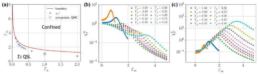
Figure 4: (a) Phase diagram of model-X. The red curve is the perturbative large-$\Gamma_{m}$ phase boundary, Eq. (11), between $\mathbb{Z}_{2}$ quantum spin liquid and the confined (paramagnetic) phase, resulting from the mapping to the $\mathbb{Z}_{2}$ lattice gauge model. Blue crosses are the boundary points from the location of maximum fidelity susceptibility calculated with ED, as shown in (b). The two open circles represent the $L\rightarrow\infty$ transition point extrapolated from the QMC data simulated at fixed $\Gamma_{g}=0.2$ and $1.0$, where the extrapolated transition points are at $\Gamma_{m}\approx 2.27$, and $\Gamma_{m}\approx 1.0$, respectively, as discussed in Sec. III.2. The Fidelity susceptibilities $\chi^{m}_{F}$ in (b) and $\chi^{g}_{F}$ in (c) were calculated using Lanczos ED with $N=2\times 2\times 6$ spins.

III Analysis of model-X

In this section, we present our numerical studies of the model-X introduced in Sec. II.2. Our results support the theoretical conjecture that the model has a topological and a paramagnetic phase with no other phases. The nature of the quantum phase transitions between these two states is revealed. In the following, we fix $J=1$ and impose periodic boundary conditions in all our numerical simulations.

III.1 Fidelity susceptibility

To confirm that the model does have phases predicted by the effective $\mathbb{Z}_{2}$ gauge theory, we start by identifying signatures of the phase transition. We first consider the fidelity susceptibility which can probe the existence of a phase transition without requiring knowledge of any order parameter You et al. (2007). The fidelity susceptibility is defined as the second derivative of the logarithmic fidelity with respect to a generic tuning parameter $x$

$$\chi_{F}=\frac{\partial^{2}\ln F_{x}}{\partial\delta_{x}^{2}}|_{\delta_{x}=0},$$ (16)

where $F_{x}=|\left<\psi(x)|\psi(x+\delta_{x})\right>|$ is the infinitesimal fidelity in the direction defined by $x$. In our model with transverse fields, two types of fidelity susceptibilities can be formally defined with variations along the two different transverse fields; $x=\Gamma_{m}$ or $x=\Gamma_{g}$;

$$\chi^{m}_{F}(\Gamma_{m},\Gamma_{g}) =\frac{\partial^{2}\ln F_{\Gamma_{m}}}{\partial\delta_{\Gamma_{m}}^{2}}|_{\delta_{\Gamma_{m}}=0},$$ (17a)

$$\chi^{g}_{F}(\Gamma_{m},\Gamma_{g}) =\frac{\partial^{2}\ln F_{\Gamma_{g}}}{\partial\delta_{\Gamma_{g}}^{2}}|_{\delta_{\Gamma_{g}}=0}.$$ (17b)

Across a phase transition, the fidelity susceptibility should develop a maximum that diverges in the thermodynamic limit.

We first calculate the fidelity susceptibilities using exact diagonalization with the Lanczos method Gu (2010); Prelovšek and Bonča (2013) on a small system with $2\times 2$ unit cells, i.e., $N=24$ spins in total. Due to the rapid growth of the Hilbert space, this is currently the largest accessible system size with our computational resources. Fig. 4(b) shows $\chi^{m}_{F}$ as a function of $\Gamma_{m}$ for several different values of $\Gamma_{g}$. A single peak is present in all cases, which implies the possibility of a phase transition in the thermodynamic limit. Furthermore, we have not observed any cases of multiple maxima in any of our calculations, suggesting only two different phases. Similar behaviors are also observed for $\chi^{g}_{F}$ as shown in Fig. 4(c). From the location of the maximum of $\chi^{m}_{F}$ shown in Fig. 4(a), we find that the data fall close to the perturbative (large-$\Gamma_{m}$) topological–paramagnetic phase boundary even though the value of $\Gamma_{m}$ is not extremely large (and $\Gamma_{g}$ not extremely small).

It may seem surprising that the phase boundary is given accurately by a system with only four unit cells. To confirm that the observed maximum of the fidelity susceptibility grows with the system size and truly indicates a phase transition, we next turn to QMC simulations to reach larger system sizes. We use the SSE QMC method Sandvik (2010, 2019), for which a convenient way to compute the fidelity susceptibility was devised recently Wang et al. (2015).

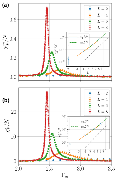
Figure 5: SSE results for the size-normalized fidelity susceptibilities $\chi^{m}_{F}/N$ (a) and $\chi^{g}_{F}/N$ (b) for systems with different number of spins $N=L\times L\times 6$. All data points for a given $L$ were obtained in the same simulation with quantum parallel tempering at fixed $\Gamma_{g}=0.2$ and inverse temperature $\beta=4L$. The insets show log-log plots of the peak value of the fidelity susceptibility versus $L$, along with solid lines drawn through pairs of data points with $L$ and $L+2$ to analyze power-law behaviors $\chi_{F}/N\sim L^{b_{L}}$. The extracted size-dependent exponents in (a) are $b_{4}\approx 3.0$ from the $L=4,6$ points and $b_{6}\approx 3.5$ from $L=6,8$. In (b) the $L=4,6$ points give $b_{4}\approx 2.7$ and $L=6,8$ give $b_{6}\approx 3.2$. The dotted lines in the insets of (a) and (b) have a slope $b=2(d+1)-d=4$ corresponding to a first-order transition and are shown as a reference.

In our simulation, we set the inverse temperature as $\beta=4L$. Because of the small vison gaps in the topological phase, this scaling of $\beta$ does not allow us to reach the finite-size ground state deep inside the topological phase. However, with the $T\to 0$ limit approached with $\beta\propto L$ we can still address the nature of the quantum phase transition from the gapped paramagnetic phase. In our model, the Ising interactions are highly frustrated, and to mitigate the associated effects of slow dynamic of the QMC updates in the topological phase and at the phase transition, we have implemented quantum replica exchange Hukushima and Nemoto (1996); Hukushima et al. (1996); Sengupta et al. (2002). Simulations are thus carried out in parallel for a large number of replicas with different values of $\Gamma_{m}$ on both sides of the transition, with swap attempts carried out for neighboring values of the parameter after several conventional SSE updates. Even with replica exchange, it is still difficult to equilibrate systems for large $L$, and we have limited the present study to $L\leq 8$. As we will see, these moderate system sizes are already sufficient for drawing definite conclusions.

Fig. 5(a) shows the results of the fidelity susceptibility $\chi^{m}_{F}$ at $\Gamma_{g}=0.2$ as a function of $\Gamma_{m}$. We indeed find that the peak identified in the ED calculations diverges upon increasing the system size, providing solid evidence of a phase transition. The other fidelity susceptibility $\chi^{g}_{F}$ shows a similar behavior, as shown in Fig. 5(b).

In order to understand the nature of the phase transition, we perform finite-size scaling of the maximum value of the fidelity susceptibility to extract the associated critical exponent. Based on the similarity of the model to the $\mathbb{Z}_{2}$ lattice gauge model, in which the transition is in the (2+1)D Ising universality class, one might naively expect a continuous transition at which the maximum should scale with system size as Gu (2010) $\chi_{F}/L^{d}\sim L^{2/\nu-d}$ with $d=2$ the spatial dimensionality and $\nu\approx 0.63$. However, we do not observe a scaling of the above form. Instead, we analyze the data using a generic scaling form $\chi_{F}/L^{d}\sim L^{b}$ with an adjustable exponent $b$. To further take into account finite-size corrections, we consider a size dependent exponent $b_{L}$ extracted from two system sizes, $L$ and $L+2$; graphically this exponent corresponds to the slope of the line drawn between two data points on a log-log scale as shown in the insets of Fig. 5.

In the case of $\chi_{F}^{m}$ in Fig. 5(a) we find $b_{4}\approx 3.0$ (i.e., the line drawn between data points for $L=4$ and $L=6$) and $b_{6}\approx 3.5$ (from $L=6,8$). In the case of $\chi^{g}_{F}$ we find $b_{4}\approx 2.7$ and $b_{6}\approx 3.2$. These exponents are significantly larger than the expected value $2/\nu-d\approx 2/0.63-2\approx 1.175$ of the (2+1)D Ising universality class, and for both susceptibilities the deviation becomes larger for the larger system sizes. It therefore appears more likely that the transition is first-order. Generally, at classical first-order transitions the same scaling forms hold as for continuous transitions, but with the exponent $1/\nu$ replaced by the dimensionality $d$ Fisher and Berker (1982); Binder and Landau (1984). In a quantum system, the replacement should be $1/\nu\rightarrow d+z$, where the appropriate value of the dynamical exponent $z$ reflects the nature of the low-energy excitations in the two coexisting phases Sen and Sandvik (2010); Zhao et al. (2019). Our results in Fig. 5 suggest a first-order behavior with $z=1$, in which case $b=2/\nu-d\rightarrow 2(d+1)-d=4$. We show this type of divergence for reference with the dotted lines in the insets of Figs. 5(a) and 5(b); this asymptotic behavior seems very plausible based on the available data.

III.2 Topological order

Next, we turn to the properties of the underlying phases. Based on the mapping to the $\mathbb{Z}_{2}$ lattice gauge model, we expect the phase with small $\Gamma_{m}$ to be a $\mathbb{Z}_{2}$ topological quantum spin liquid. Note that Elitzur’s theorem forbids any spontaneous symmetry breaking of local gauge symmetries; thus one cannot define any local order parameter to characterize such topological order Elitzur (1975); Kotecký (1992); Kogut (1979). To detect the topological order, we investigate the global, non-contractible Wilson loop operator, defined as the product of gauge spin $\sigma^{z}$ operators along a non-contractible loop in the $\alpha$-direction

$$p_{\alpha,n}=\prod_{\{i\}_{\alpha,n}}\sigma_{i}^{z},~{}~{}~{}\alpha\in\{x,y\},$$ (18)

for the set of sites $\{i\}_{\alpha,n}$ belonging to the $n$-th row or column. For a $\mathbb{Z}_{2}$ spin liquid, the quantum numbers $p_{x,n}=\pm 1$, $p_{y,n}=\pm 1$ characterize the four degenerate (in the thermodynamic limit) topological ground states regardless of which row or column $n$ is chosen. We can take advantage of this property to define a correlation function detecting the topological order using the product of two parallel non-contractible loops on rows or columns labeled by $m$ and $n$:

$$c_{p}^{\alpha}(r_{mn})=\langle p_{\alpha,m}p_{\alpha,n}\rangle=\left(\prod_{\{i\}_{\alpha,m}}\sigma_{i}^{z}\right)\left(\prod_{\{i\}_{\alpha,n}}\sigma_{i}^{z}\right),$$ (19)

which we also illustrate in the inset of Fig. 6. Instead of investigating this correlation as a function of the distance $r_{mn}$ between the two loops, we here take the longest distance for a given lattice size, $r_{mn}=L/2$, and analyze the $L$ dependence of $C_{p}(L/2)$ defined as a summation over all translations (to reduce the statistical fluctuations) of the two Wilson loops oriented in the $\alpha\in\{x,y\}$ lattice direction:

$$C_{p}(L/2)\equiv\frac{1}{L}\sum_{j=1}^{L}c_{p}^{\alpha}(r_{j,j+L/2}),$$ (20)

which can be averaged over the two directions. In the topologically ordered phase we expect $C_{p}(L/2)\neq 0$ when $L\to\infty$, while in the paramagnetic phase $C_{p}(L/2)\to 0$. Note that this quantity has been used in a previous study of topological order in classical Ising gauge models at zero and non-zero temperatures Xu et al. (2018).

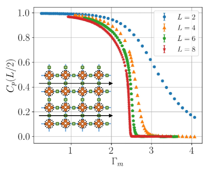
Figure 6: Wilson-loop correlation function obtained in SSE simulations with $\Gamma_{g}=0.2$. Data for different system sizes show convergence to a finite value for $\Gamma_{m}\gtrsim 2.3$, with the expected value $C_{p}(L/2)=1$ in the $\Gamma_{m}\to 0$ limit. The inset illustrates the definition Eq. (20) of the correlation function in terms of two parallel non-contractible Wilson loops in the $x$ direction of a periodic lattice of size $L=4$.

In Fig. 6, we show SSE results at $\Gamma_{g}=0.2$ as a function of $\Gamma_{m}$. We see that $C_{p}(L/2)$ indeed vanishes with increasing $L$ for large $\Gamma_{m}$, while it converges to a finite value for $\Gamma_{m}$ in a range consistent with the transition point found above for the same value of $\Gamma_{g}$. Below we will discuss the size-extrapolated phase boundary. We stress here that the Wilson loop order parameter does not detect any phases with only local order parameters (See Appendix. D for a study of the ferromagnetic state as an example) and our results therefore demonstrate conclusively a $\mathbb{Z}_{2}$ topological phase of finite extent as the field $\Gamma_{m}$ is turned on.

Having established a good topological order parameter, we further provide evidence of a first-order phase transition by a finite-size scaling analysis of the corresponding Binder ratio. To this end, we define the topological order parameter on the entire system as the sum of Wilson loops with $P^{2}=P_{x}^{2}+P_{y}^{2}$ where

$$P_{\alpha}=\frac{1}{L}\sum_{n=1}^{L}p_{\alpha,n},$$ (21)

with $\alpha\in\{x,y\}$, and the Binder ratio

$$B=\frac{\langle P^{4}\rangle}{\langle P^{2}\rangle^{2}}.$$ (22)

In a perfect $\mathbb{Z}_{2}$ ordered topological phase, $P_{x}=\pm 1$ and $P_{y}=\pm 1$, forming a $\mathbb{Z}_{2}\times\mathbb{Z}_{2}$ symmetric order parameter distribution, while $P_{x}=P_{y}=0$ in the paramagnetic phase. With increasing system sizes, the Binder ratio is expected to form a step function at the transition point in the case of a continuous transition, while the distribution of the order parameter in the coexistence state at a first-order transition typically is also associated with a divergent peak adjacent to the step Vollmayr et al. (1993); Iino et al. (2019). In Fig. 7(a) the Binder ratio indeed evolves into a step function with a side peak, though the latter is only seen clearly for the largest system sizes, $L=8$, and for $L=6$ there is a very weak maximum as well. Looking at the derivative of $B$, in Fig. 7(b) we observe a divergent positive main peak, and for $L=8$ a prominent negative peak reflects the presence of the first-order side peak in Fig. 7(a). Thus, we have strong evidence of phase coexistence at a first-order quantum phase transition caused by an avoided level crossing. In Appendix E, we further show the full distribution of the two-component Wilson loop order parameter $\rho(P_{x},P_{y})$, which clearly shows a phase coexistence characteristic of a first-order transition.

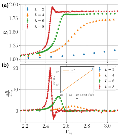
Figure 7: Results for the model with transverse field at $\Gamma_{g}=0.2$. (a) The Binder ratio $B$ defined with both components of the Wilson loop order parameter $P^{2}=P_{x}^{2}+P_{y}^{2}$ in Eq. (22). The peaks adjacent to the phase transition for system sizes $L\geq 6$ (barely discernible for $L=6$) are signatures of a first-order transition. (b) The numerical derivative of $B$ with respect to $\Gamma_{m}$ [computed using the linear approximation between the successive points in (a)]. The inset shows a power-law fit $y\propto L^{b}$ to the maximum value of the derivative, with only the largest three system sizes included. The exponent is $b\approx 3.0$, which is consistent with expected value $b=d+1=3$ for a first-order transition.

The maximum of the Binder ratio derivative diverges with the system size as the step function develops. The derivatives can be evaluated directly in the SSE simulations, using an estimator derived in Appendix B. With the replacement $1/\nu\to d+z$ in the scaling form $dB/d\Gamma_{m}\sim L^{1/\nu}$ and expecting $z=1$ here, the peaks should diverge as $L^{3}$. Indeed, in Fig. 7(b) the peak values for the three largest system sizes can be fitted to a power-law $L^{b}$ with $b\approx 3.0$, thus supporting a first-order transition.

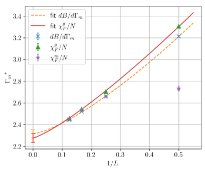
Figure 8: Scaling with the inverse system size of the $\Gamma_{m}$ values of the finite-size maxima $dB/d\Gamma_{m}$, $\chi^{m}_{F}/N$ and $\chi^{g}_{F}/N$, with $\Gamma_{g}=0.2$. Both $dB/d\Gamma_{m}^{*}$ and $\chi^{g*}_{F}/N$ have been fitted with a single power-law correction and give the $L\to\infty$ extrapolated values $\Gamma_{m}^{c}=2.31(3)$ and $\Gamma_{m}^{c}=2.27(4)$, respectively. The apparent large subleading corrections to $\chi^{m*}_{F}$ location forbid us to get a reasonable extrapolation based on the available data, though the $L=6$ and $L=8$ pints show full consistency with the other estimates.

So far, we have discussed the divergence properties of the peaks in the Binder ratio and the fidelity susceptibility. We also need to extrapolate the peak locations in order to obtain the transition point in the thermodynamic limit. Fig. 8 shows the dependence of the peak locations on $1/L$ along with extrapolations assuming power-law corrections. All quantities show mutually consistent behaviors for the largest system sizes, but $\chi_{F}^{m}$ has much larger scaling corrections than the other quantities. Extrapolations with error analysis give the critical value of the matter field $\Gamma_{m}^{c}\approx 2.27$ for the gauge field $\Gamma_{g}=0.2$ considered here. In the phase diagram in Fig. 4(a) we have marked this transition point with a circle, and we also show the result obtained using the same methods for $\Gamma_{g}=1$. These QMC points are very close to the boundary estimated from the ED results for a very small system with $L=2$.

Here we should note that the ED results are calculated exactly at $T=0$, while there are still some temperature effects left in the QMC results obtained with our choice of temperature scaling, $T=(4L)^{-1}$. In the case of $L=2$, the QMC results for $\Gamma_{m}^{c}(L)$ are actually quite far from the $T=0$ ED results because of the temperature effects. However, since $T\to 0$ as $L$ increases, the $L\to\infty$ extrapolated QMC results are not affected by finite temperature (beside unimportant constant factors in the peaks of the physical quantities). In this regard, it can also be noted that effects of inappropriate temperature scaling with $L$ could potentially ruin a quantum phase transition that does not extend to $T>0$ (as is the case with topological order in two spatial dimensions), while there is no reason to expect a transition detected when $T\propto 1/L$ to vanish if $T$ approaches zero more rapidly.

III.3 Energy derivative

In this section, we show another signature of the first-order phase transition from the ground state energy density. In practice, the $T\to 0$ internal energy is obtained with QMC calculations at $T=(4L)^{-1}$. The type of first-order transition indicated by the results above, where finite-size scaling with the exponent replacement $1/\nu\to d+z$ holds, should be associated with an avoided level crossing. Thus we expect a change in the slope of the energy at the transition with increasing $L$. In Fig. 9(a) we plot the energy per site as a function of $\Gamma_{m}$ for the same gauge-field strength as considered above, $\Gamma_{g}=0.2$. At first sight, the data exhibit a smooth behavior without any visible kink. However, by taking the numerical derivative of the energy, as shown in Fig. 9(b), we find a clear signature of non-analytic behavior, such that the derivative becomes discontinuous at the transition in the thermodynamic limit.

Along with the other results, this demonstration of a discontinuous energy derivative provides definite proof of a first-order quantum phase transition between the topological and paramagnetic states.

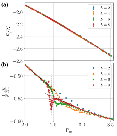
Figure 9: (a) Energy density computed in SSE simulations with $\Gamma_{m}=0.2$. (b) The corresponding derivatives are taken numerically based on the available data in (a). Features indicating a discontinuity developing with increasing $L$ demonstrate a first-order transition. We have fitted lines to the $L=8$ data away from the sharp features and observe the presence of a jump when these forms are extrapolated to the location of the sharp peak (the vertical dashed line, which can be taken as a finite-size definition of the transition point).

III.4 Level spectroscopy

Having used QMC simulations to establish the existence of an extended $\mathbb{Z}_{2}$ topological phase and its quantum phase transition into the paramagnetic phase, we now again turn to Lanczos ED calculations in order to investigate the energy level spectrum of the system. We use the combinatorial $\mathbb{Z}_{2}$ symmetry to block-diagonalize the Hamiltonian into $M=2+L^{2}-1$ blocks in the basis of $\mathbb{Z}_{2}$ gauge generators, as discussed in detail in Appendix A. The blocks are categorized by a set $\mathbf{q}=(\pm,\pm,\{\pm\})$ of quantum numbers, where the first two elements correspond to the two non-contractible loops with associated quantum numbers $G_{x}$ and $G_{y}$ and $\{\pm\}$ denotes the set of $L^{2}-1$ local quantum numbers $G_{i}$. In the thermodynamic limit, the topological ground state should be four-fold degenerate, corresponding to the lowest energy states from sectors with $G_{x}=\pm$, $G_{y}=\pm$ and $G_{i}=+$ for all other $i\in M-2$ local operators. The transverse field does not commute with the Hamiltonian; thus, there are always finite-size gaps between the four topological states in a finite system. Our ED calculations here are again restricted to $L=2$ (and we present some QMC results also for $L=4$), but even for this very small system many of the salient signatures of spinon and vison excitations can be observed, as well as signatures of the first-order quantum phase transition.

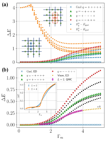
Figure 10: ED level spectrum at $\Gamma_{g}=0.2$ for a system of size $L=2$ ($N=2\times 2\times 6$ spins). In (a) the two lowest energy gaps relative to the ground state (marked Gnd in the legends) are graphed versus the matter field strength for each of the 32 blocks with quantum numbers $\mathbf{q}=(\pm,\pm,\pm,\pm,\pm)$. Many blocks are degenerate because of lattice symmetries; thus the number of different curves is much less than 64. The four states that become degenerate topological ground states in the $\mathbb{Z}_{2}$ phase are marked by blue crosses (the finite-size ground state), red stars, and green triangles (two degenerate sectors); these states all have the local quantum numbers $G_{i}=+1$. The blue dots represent all other lowest block levels; these are states with visons (two or a larger even number) of the topological phase (marked by $v$ in the inset illustration). The orange curves represent the second-lowest states in each block; they correspond to the spinon excitations (particles indicated in the inset by $s$) of the topological phase and they all become degenerate for $\Gamma_{m}\to 0$. In (b), the lowest block states are graphed on a magnified scale. The eight-fold degenerate level that is the lowest excitation in the paramagnetic phase was calculated with both ED (yellow dots) and extracted from imaginary-time correlations from QMC simulations (violet circles), to demonstrate the correctness of the latter for $L=2$. QMC results for both $L=2$ and $L=4$ (calculated at inverse temperature $\beta=24L$) are shown in the inset.

In Fig. 10(a), we graph low-energy gaps $\Delta_{E}$ relative to the ground state versus the matter field $\Gamma_{m}$ at fixed $\Gamma_{g}=0.2$. For each of the 32 topological symmetry blocks pf the $L=2$ system, the two smallest gaps are shown, but because of degeneracies due to lattice symmetries there are only 11 distinct curves. The unique finite-size ground state has $\mathbf{q}=(+,+,+,+,+)$, i.e., $G_{x}=+$, $G_{y}=+$ and $G_{i}=+$ for $i=1,2,3$. The four levels that become degenerate in the thermodynamic limit in the topological phase are highlighted with different symbols. As for the remaining low-energy levels, we note that in the $\mathbb{Z}_{2}$ topological phase two types of quasi-particle excitations should be expected; spinons ($s$) and visons ($v$), which are created in pairs by acting on the ground state with $\sigma^{x}$ and $\sigma^{z}$ respectively on the gauge spins, as indicated in the insets of Fig. 10(a).

In the $\Gamma_{m}\rightarrow 0$ limit, the spinon excitations are gapped with $\Delta_{E}\approx 4J$ (the gap value is $4J$ if $\Gamma_{g}=0$), as seen clearly in Fig. 10(a), where these levels are shown with orange symbols. The vison gap opens when increasing $\Gamma_{m}$, as can be seen from the fact that the effective model takes the form

$$H_{pert}=\sum_{s}H_{s}-g\sum_{p}G_{p}$$ (23)

to lowest order in perturbation theory. Here $G_{p}$ is the local gauge generator that appears at 12th order, where the coupling is

$$g\propto\left(\Gamma_{m}^{8}\Gamma_{g}^{4}\right)/J^{11}.$$ (24)

We can identify the vison excited states simply by considering the quantum number blocks that couple to the ground state through the on-site $\sigma^{z}$ operators (which do not commute with the local gauge operators). In Fig. 10(b), we plot ED results for the same parameters as in Fig. 10(a), but with a change in scale to focus on the vison states. These states are gapped for all $\Gamma_{m}>0$, but the gaps are much smaller in the topological phase than in the paramagnetic phase. The lowest vison state, which contains two visons, is eight-fold degenerate on the small system considered here. The other levels in Fig. 10(b) correspond to states with (an even number) more than two visons.

We can extract the lowest vison gap from QMC simulation by analyzing the imaginary-time autocorrelation function of $\sigma_{z}$, defined as

$$G(\tau)=\frac{1}{N_{g}}\sum_{i\in g}\left<\sigma^{z}_{i}(0)\sigma^{z}_{i}(\tau)\right>,$$ (25)

where $N_{g}=L\times L\times 2$ is the total number of gauge spins in the system. The gap can be extracted by fitting an exponential function to $G(\tau)$ for large $\tau$. Here it is also important that the temperature is sufficiently low, so that the asymptotic form of $G(\tau)$ is dominated by the lowest gap; See Appendix. C for further technical details on these calculations. In Fig. 10(b) we compare the lowest gap extracted from the QMC data for the $L=2$ system at inverse temperature $\beta=48$ with the ED result. We observe good agreement between the two calculations. Note that the eight-fold degenerate levels with two vison excitations undergo a true (not avoided) level crossing with a state with $G_{x}=G_{y}=+$ and all local quantum numbers $G_{i}=-$. This level-crossing is a finite-size effect, and we do not expect such behavior to persist for larger system sizes. The $G_{i}=-$ state contains four visons, i.e., it can be reached from the ground state with two different $\sigma^{z}_{i}$ operations. It therefore does not contaminate the correlation function $G(\tau)$ corresponding to the two-vison level of interest. For this small system the four-vison state falls under the lowest 2-vison state below $\Gamma_{m}\approx 3$, i.e., close to the phase transition into the topological state.

Note again that the quantum numbers $G_{i}$ are conserved (i.e. commute with the Hamiltonian) in both the topological phase and the paramagnetic phase of the model. However, visons with $G_{i}=-$ are deconfined only in the topological phase. In the paramagnetic phase, the lowest energy vison excitations must form bound states residing on two adjacent plaquettes, while states with more visons and larger separations between the visons have larger energy costs, as shown in Fig. 10(b).

In the inset of Fig. 10(b), we show the vison gap based on QMC calculations for both $L=2$ and $L=4$ at $\Gamma_{m}=0.2$, using inverse temperature $\beta=24L$. While the $L=2$ gap exhibits only a rather smooth variation with $\Gamma_{m}$, at $L=4$ a sharp feature has developed close to the phase transition. The sharp behavior of the gap here is consistent with the scenario of a first-order transition through an avoided ground state level crossing, and this mechanism should be associated also with avoided level crossings of the low-lying excitations.

Although the model possess $\mathbb{Z}_{2}$ topological order and can be directly implemented on existing quantum devices Zhou et al. (2020), it will be difficult to reach the true ground state, or even a thermal state with a low density of visons, due to the very small vison gap. These difficulties are clear from the effective model obtained perturbatively, Eq. (23) with the 12th-order effective coupling in Eq. (24). Nonetheless, there may still be signatures of the mutual statistics of the spinons and visons that could be observed in the regime where temperature is larger than the vison gap but still much smaller than the spinon gap, as discussed in Ref. Hart et al. (2021). In this regime the visons randomly appear within plaquettes because their energy of formation is much smaller than the temperature. In the presence of kinetic terms (such as a transverse field), the spinons acquire dynamics at a scale much faster than that of the visons, so effectively they quantum diffuse in a background or randomly placed visons. Because of the mutual statistical phase of $\pi$ between the two types of particles, the random visons serve as sources of $\pi$ fluxes, which lead to quantum interference corrections to the diffusion of the spinons.

IV Analysis of model-XX

Here we present numerical results for the model-XX introduced in Sec. II.3, organized in the same way as the numerical studies of model-X in Sec. III. Lanczos ED calculations were carried out for $L=2$ systems. QMC results for larger systems up to $L=6$ were again obtained using the SSE method supplemented with quantum replica exchange. We fixed $\Gamma_{m}=1.0$ and simulated several replicas at different values of $J_{x}$ across the two phases. The values are chosen such that the acceptance rate of swapping neighboring replicas is in the range $0.4\sim 0.6$. Our findings and arguments are very similar to those for model-X discussed in Sec. III, with the exception of issues pertaining to the ferromagnetic phase, and we therefore keep the discussion brief in this section.

IV.1 Fidelity susceptibility

As in the previous study of model-X, we first discuss Lanczos ED results for the fidelity susceptibility $\chi^{x}_{F}$ defined as in Eq. (17b) with the substitution $\Gamma_{g}\rightarrow J_{x}$. In Fig. 11(b), we show $\chi^{x}_{F}$ versus $J_{x}$ for several values of $\Gamma_{m}$. In all cases, we observe a peak indicative of a phase transition. The locations of the maxima are shown along with the perturbative phase boundary in Fig. 11(a).

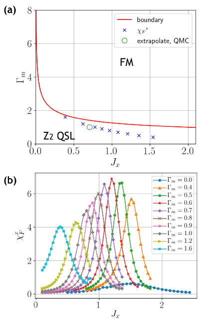
Figure 11: (a) Phase diagram of the model with XX interactions. The red curve is the approximate phase boundary obtained from the asymptotic $\Gamma_{m}\to\infty$ mapping to the TFIM. This boundary separates the $\mathbb{Z}_{2}$ topological quantum spin liquid and the ferromagnetic phases. The blue crosses are points on the boundary estimated from the maximum of the fidelity susceptibility in (b), calculated using ED on an $L=2$ system. The green open circle indicates the $L\rightarrow\infty$ extrapolated transition point $J_{x}\approx 0.706$ from QMC simulations at $\Gamma_{m}=1.0$.

In Fig. 12(a) we plot SSE results for larger systems. As expected we find a maximum that diverges with increasing system size, showing a true phase boundary and only two phases. Analyzing the peak height using the effective exponent $b_{L}$ defined with system sizes $L$ and $L+2$, we find $b_{2}\approx 4.8$ and $b_{4}\approx 3.9$. These exponents are again significantly larger than the $2/\nu-d\approx 2/0.63-2\approx 1.175$ for the (2+1)D Ising universality class, but close to $b=2(d+z)-d=4$ for a first-order transition when $z=1$. We note one difference with respect to the previous model, as seen in Fig. 5, in that case the exponent $b_{L}$ increases with $L$, while in the present case it decreases. One may then question whether the value $b=4$ is really obtained in the limit $L\to\infty$. Nevertheless, all our complementary results to be presented below also lend support to a first-order transition.

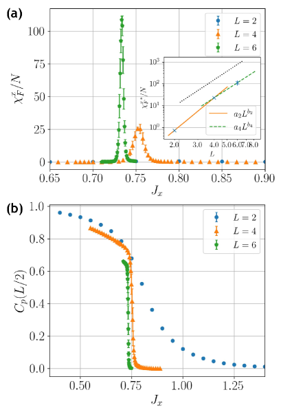
Figure 12: (a) Fidelity susceptibility of model-XX at $\Gamma_{m}=1.0$ for different system sizes $L$ calculated using SSE simulation at inverse temperature $\beta=4L$. The inset shows power-law fits $y\propto L^{b_{L}}$ to the maximum values for system sizes $L$ and $L+2$. The exponents are $b_{2}\approx 4.9$ and $b_{4}\approx 3.9$. The slope of dotted line corresponds to the predicted exponent $b_{\infty}=2(d+1)-d=4$ expected for a first-order transition. (b) QMC results at $\Gamma_{m}=1.0$ for the Wilson loop correlation function, Eq. (20).

IV.2 Topological order

To detect the topological order, we again consider the correlation function $C_{p}(L/2)$ between two parallel non-contractible Wilson loops, defined previously in Eq. (20). Fig. 12(b) shows results at $\Gamma_{m}=1.0$. Here a discontinuity reflecting the first-order transition develops more clearly as compared to the results for model-X in Fig. 6, thus suggesting a more strongly first-order transition in this case. Note, however, that the parameter values chosen for the two models in these figures, $\Gamma_{g}=0.2$ and $\Gamma_{m}=1$, are not directly comparable. In both cases, the strength of the discontinuity will vary with the model parameters.

As in Sec. III, we use the Wilson loop order parameters $P_{x}=\sum_{a}p_{x,a}$ and $P_{y}=\sum_{a}p_{y,a}$ to confirm the extent of the topological phase. We use the Binder ratio $B$ as defined in Eq. (22) with both components taken into account. The results, shown in Fig. 13(a) exhibit developing step functions with associated peaks indicative of a first-order transition. The derivatives exhibit the expected divergent peaks. Because of the limited system sizes, we refrain from analyzing the peaks further. We have used the peaks to extrapolate the transition point to infinite size and show the result with the green circle in the phase diagram in Fig. 11 at $\Gamma_{m}=1$. As in the model-X with transverse field on the gauge spins, we find only a small difference between the QMC result and the $L=2$ ED result in this case.

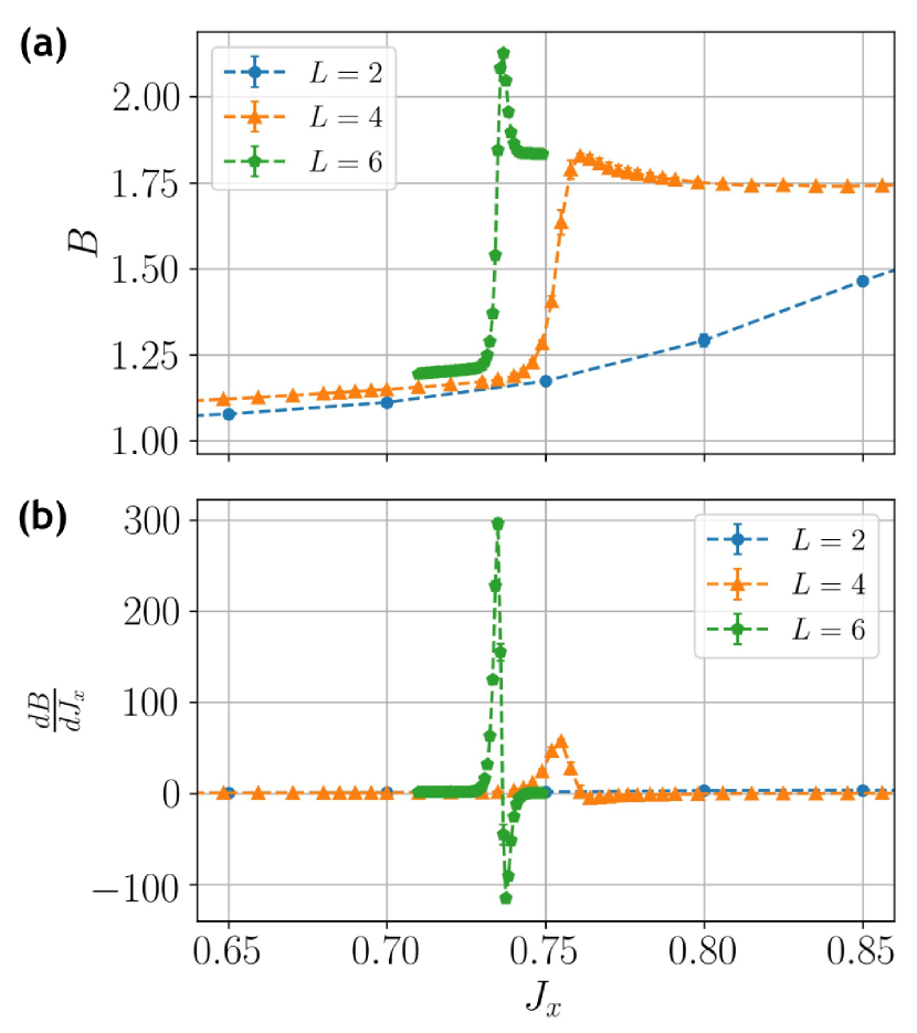
Figure 13: Results for model-XX at $\Gamma_{m}=1.0$. (a) The Binder ratio of the Wilson loop order parameter defined with both components in Eq. (21); $P^{2}=P_{x}^{2}+P_{y}^{2}$. The divergent peak next to the step indicates phase coexistence at a first-order transition. Accordingly, in (b) the derivative of the Binder ratio shows divergent positive and negative peaks.

IV.3 Energy derivative

We present further evidence of a first-order phase transition from the energy density. As shown in Fig. 14(a), in this case we observe a clear kink behavior for the larger system sizes, $L\geq 4$, and the derivative in Fig. 14(b) accordingly shows a strong discontinuity developing.

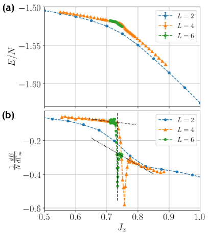
Figure 14: (a) Energy per spin of model-XX obtained in the same simulations as the other quantities at $\Gamma_{m}=1.0$ and temperature $T=(4L)^{-1}$. (b) The derivatives are evaluated using the linear approximation using the data in (a). The dotted lines are fits to the $L=4$ results away from the peak and demonstrate a jump in the energy derivative at the transition (here represented by the peak location as indicated by the vertical dashed line).

IV.4 Level spectroscopy

We have again used Lanczos ED to find low-lying states for each block of quantum numbers characterizing the combinatorial $\mathbb{Z}_{2}$ symmetries in the $L=2$ system. In Fig. 15, we present the two smallest gaps versus the XX coupling $J_{x}$ at $\Gamma_{m}=1.0$. The lowest states in the sectors $G_{x}=\pm$, $G_{y}=\pm$ and $G_{i}=+$ again are those that will eventually become degenerate as $L\rightarrow\infty$ in the topological phase, and these states are highlighted with different symbols. The lowest energy excitations in the topological phase, states with visons, form levels very similar to what we saw in the model-X. However, the spinon spectrum looks very different. Due to the $XX$ ferromagnetic interaction, spinons created in pairs within one of the sublattices has lower energy comparing to the one created in neighboring pairs (created by a single $\sigma_{x}$ operation) as illustrated in Fig. 15(a).

At $J_{x}\rightarrow 0$, only spinon excitations exist, with a gap size of order O($J$), as can be seen in Fig. 15(a) where these levels are marked in orange. The vison gap opens with increasing $J_{x}$, as the effective model from the lowest order in perturbation takes the form

$$H_{\rm pert}=\sum_{s}H_{s}-g\sum_{p}G_{p}.$$ (26)

Here $G_{p}$ is the local gauge generator (plaquette term) that appears at 10th order, with $g\sim\Gamma_{m}^{8}J_{x}^{2}/J^{9}$, which should be compared to the 12th order perturbative Hamiltonian in the case of model-X.

In the case of the XX interaction used here, there is an additional gauge spin inversion symmetry in $x$-basis that is not present in the model-X. Define the inversion operator $V=\prod_{i}\sigma_{i}^{z}$ as the product of all $\sigma^{z}$ gauge-spins. This operator clearly commute with Hamiltonian and its quantum numbers $v=\pm$ correspond to symmetric or antisymmetric states. We find that all the lowest energy levels of the 32 gauge blocks (blue) are symmetric and the second state (orange) is always anti-symmetric except for the highest energy level shown in Fig. 15(a), which exhibits an actual level crossing (see appendix  F for further details).

Among all the spinon excitations, the lowest one belongs to the same sector as the ground state, with $\mathbf{q}=+++++$. This excitation, which is marked with a dashed line in Fig. 15(a), becomes degenerate with the ground state for large $J_{x}$, reflecting the ferromagnetic Ising order with spontaneously broken $\mathbb{Z}_{2}$ symmetry in the thermodynamic limit.

For the vison excitations, since $\sigma^{z}$ operators do not commute with local gauge operators, we can identify the vison excited states simply by considering the quantum number blocks that couple to the ground state through the on-site $\sigma^{z}$ operators. In Fig. 15(b), we plot ED results for the same parameters as in Fig. 15(a), but with a change in scale to focus on the vison states. These states are gapped for all $J_{x}>0$, but the gaps are much smaller in the topological phase than in the FM phase. The lowest vison state, which is marked by yellow symbols in Fig. 15(b), contains two $m$ particles, and is eight-fold degenerate on the small system considered here. The other levels marked by blue in Fig. 15(a) correspond to states with more than two (an even number of) visons.

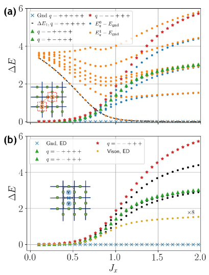
Figure 15: Level spectrum relative to the ground state for the $L=2$ system with XX interactions, calculated with Lanczos ED. The organization of panels (a) and (b) is as in the corresponding Fig. 10 for the model-X. We refer to the same for further explanation of the visualization of the spectrum. The lowest spinon excitation, shown as orange circles with a dashed line, is the first excited state from the same block as the ground state (which has $\mathbf{q}=+++++$). This state is antisymmetric with respect to spin inversion and forms the two-fold degenerate multiplet together with the corresponding symmetric state in the ferromagnetic phase.

V Conclusions and Discussion

We have presented a numerical study of spin models with only one- and two-spin interactions that realize a combinatorial $\mathbb{Z}_{2}$ gauge symmetry. We considered two models that only differ by the kinetic terms given to the gauge spins: model-X (containing a transverse field) and model-XX (containing $XX$ interactions). We found conclusive evidence for an extended $\mathbb{Z}_{2}$ topological quantum spin liquid phase in both models.

In the case of model-X, we identified two phases; a topological phase and a paramagnetic phase. We demonstrated a first-order quantum phase transition between these phases, in contrast to the well known continuous transition of the conventional $\mathbb{Z}_{2}$ lattice gauge model. In model-XX we identified a topological phase and a competing ferromagnetic state. Our data also support a first-order transition between these two phases in model-XX. Perturbatively, the $XX$ interaction of model-XX generates a plaquette operator $G_{p}$ at a lower order in perturbation theory as compared to the transverse field of model-X, and therefore the size of the vison gap increases, as we also observe.

The presence of the first-order transition between the topological and the competing state, in both models, raises the following interesting question: As we have discussed in the paper, in the limit of a large transverse field $\Gamma_{m}$ on the matter spins, the models map to the usual Ising gauge model, which has a continuous transition. An important question is then whether the continuous transition persists for some finite range of values of $\Gamma_{m}$, or whether it turns first-order immediately. This question can in principle be answered by considering the corrections to the usual $\mathbb{Z}_{2}$ gauge model in Eq. (10), which will appear when carrying out a perturbative expansion to higher order in $\Gamma_{m}^{-1}$. The question is then whether these corrections are renormalization-group relevant or irrelevant at the critical point. While we have not carried out this expansion and duality mapping, it appears likely that the additional interactions generated in the Ising model will involve products of more than two spins, and most likely these interactions will be irrelevant at the Ising critical point. Thus, we suspect that there will be indeed a tricritical point separating continuous Ising transitions and first-order transitions for large values of $\Gamma_{m}$ in Figs. 4 and 11. We leave tests of this hypothesis open for future work.

Appendix A $\mathbb{Z}_{2}$ gauge symmetry and conserved quantum numbers

Recall that in the $\mathbb{Z}_{2}$ lattice gauge theory,

$$H_{\mathbb{Z}_{2}}=J\sum_{i}A^{z}_{i}-h_{x}\sum_{i}\sigma_{x}^{i}$$ (27)

where $A^{z}_{i}$ is the star operator defined as $A^{z}_{i}=\sigma_{z}^{1}\sigma_{z}^{2}\sigma_{z}^{3}\sigma_{z}^{4}$ acting on 4 spins emanating from a single site as shown in Fig. 2(b). The local gauge generator $G=\prod\sigma_{x}$ is defined as a product of $\sigma_{x}$ operators around an elementary plaquette [shown as the blue cross in Fig. 2(b)], which is a conserved quantity of the system, i.e. $G\ket{E_{q}}=q\ket{E_{q}}$ where $\ket{E_{q}}$ is an energy eigenstate. Thus we can use these operators to characterize the quantum number sectors.

In analogy to the standard $\mathbb{Z}_{2}$ lattice gauge theory, in our model the 4-body interaction term $A_{i}$ is effectively generated with the term (See Ref. Chamon et al. (2020) for further details)

$$J\sum_{a\in s}\left(\sum_{j\in s}W_{aj}\sigma^{z}_{j}\right)\mu^{z}_{a}\rightarrow-\gamma-\lambda\sum_{i\in s}\sigma_{i}^{z},$$ (28)

and the monomial transformation leads to the modification of the local gauge generator

$$G_{p}=\prod_{s\in p}\mathcal{L}_{s}^{\mu}\prod_{i\in p}\sigma_{i}^{x},$$ (29)

with the additional $\mathcal{L}_{s}^{\mu}$ representing the action of monomial matrices $\mathcal{L}$ acting on matter spins. All the formulations that characterize the symmetry and quantum numbers in the standard $\mathbb{Z}_{2}$ lattice gauge theory can also be applied to our model with combinatorial $\mathbb{Z}_{2}$ gauge symmetry.

There are in total $M=2+(L_{x}L_{y}-1)$ such independent operators in a $L_{x}\times L_{y}$ system with periodic boundary conditions. Within the $M$ operators, two of them are defined as a product of $\sigma_{x}$, $G_{i}\equiv\prod_{j}^{(i)}\sigma_{x}^{j}$ along non-contractible loops where their quantum numbers uniquely characterize the 4-fold topological degeneracies of the ground state in the thermodynamic limit. As shown in Figure. 16(a), $G_{y}$ is defined along a non-contractible loop in the $y$-direction, and $G_{x}$ is defined in the $x$-direction. Other operators are local, defined as a product of $\sigma_{x}$ around an elementary plaquette of 4 spins.

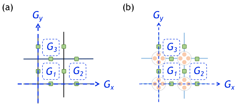
Figure 16: (a) Definitions of $M$ independent gauge operators in the conventional $\mathbb{Z}_{2}$ model for a system of size $2\times 2$. (b) The corresponding operators define on the lattice of combinatorial $\mathbb{Z}_{2}$ model. Here, $G_{x}$ and $G_{y}$ are the gauge operators defined on non-contractible loops along x and y direction respectively.

Using the fact that $G$ commutes with the Hamiltonian, we can construct eigenstates of the $G$ operators: $G\ket{q}=q\ket{q}$ where $q=\pm 1$. It is straightforward to see that for each $G$ operator, the eigenstate can be constructed by starting from a classical configuration (which we refer to as the “representative” state Sandvik (2010)) via $\ket{q}=(1+qG)\ket{\mathrm{rep}}$. Since the Hamiltonian commutes simultaneously with all $M$ operators, the state should be constructed with a product of $1+q_{i}G_{i}$ for all $G_{i}$. As an example, consider a $2\times 2$ system as shown in Fig. 16, we have

$$\ket{\mathbf{q}_{i}}=\frac{1}{Z}(1+q_{x}G_{x})(1+q_{y}G_{y})\prod_{j=1}^{3}(1+q_{j}G_{j})\ket{\mathrm{rep}_{i}}$$ (30)

where $\mathbf{q}$ indicates the quantum number set $\mathbf{q}=(q_{x},q_{y},q_{1},q_{2},q_{3})=(\pm,\pm,\pm,\pm,\pm)$, $Z$ is the normalization factor and subscript $i$ indicates the $i$-th state within the block. There are in total $2^{M}$ symmetry blocks in the system.

Appendix B SSE derivative of the Wilson loop Binder ratio

The derivative of the Binder ratio can be evaluated directly in SSE simulations, using the estimator derived here. Consider the Hamiltonian $H=JH_{0}+\delta H_{\delta}$, where $\delta$ is the tuning parameter and $[H_{0},H_{\delta}]\neq 0$. For any arbitrary diagonal observable $O$, the expectation can be express in the SSE representation as Sandvik (2010)

$$\left<O\right> =\frac{1}{Z}\sum_{\{\alpha_{i}\}}F(\beta,n)O_{\alpha_{0}\alpha_{0}}H^{\alpha_{0}\alpha_{1}}\cdots H^{\alpha_{M-1}\alpha_{0}}$$

$$=\frac{1}{Z}\sum_{\{\alpha_{i}\}}F(\beta,n)O_{\alpha_{0}\alpha_{0}}J^{n_{J}(\{\alpha_{i}\})}\delta^{n_{\delta}(\{\alpha_{i}\})}R\left[H_{a_{i},b_{i}}\right]$$ (31)

where

$$F(\beta,n)\equiv\frac{\beta^{n}(M-n)!}{M!},$$ (32)

and we have used the short-hand notation $H^{\alpha_{i}\alpha_{j}}=\left<\alpha_{i}|H|\alpha_{j}\right>$ and $O_{\alpha_{0}\alpha_{0}}=\left<\alpha_{0}|O|\alpha_{0}\right>$. Further, $Z$ is the partition function, $M$ is the operator string length and $n$ is the number of non-identity operators in the current string. The quantity denoted $R\left[H_{a_{i},b_{i}}\right]$ stands for the product of local Hamiltonian operators, $\prod_{i}H_{\alpha_{i}}$, where $H_{\alpha_{i}}=H_{0}^{i}$ or $H_{\delta}^{i}$.

The derivative of the observable with respect to the tuning parameter $\delta$ can be calculated from

$$\frac{\partial\left<O\right>}{\partial\delta} =\frac{\left<On_{\delta}\right>}{\delta}-\left<O\right>\frac{\left<n_{\delta}\right>}{\delta}$$

$$=\frac{\left<On_{\delta}\right>-\left<O\right>\left<n_{\delta}\right>}{\delta},$$ (33)

where $n_{\delta}$ is the number of the $\delta$ operators in the string. We are interested in the Binder ratio of the Wilson loop order parameter, defined as in Eq. (22). Using the above expressions we obtain

$$\frac{\partial B}{\partial\delta} =\frac{\partial_{\delta}\left<P^{4}\right>}{\left<P^{2}\right>^{2}}-\frac{2\left<P^{4}\right>\left<P^{2}\right>\partial_{\delta}\left<P^{2}\right>}{\left<P^{2}\right>^{4}}$$

$$=\frac{1}{\delta}\left[\frac{\left<P^{4}n_{\delta}\right>+\left<P^{4}\right>\left<n_{\delta}\right>}{\left<P^{2}\right>^{2}}-\frac{2\left<P^{4}\right>\left<P^{2}n_{\delta}\right>}{\left<P_{x}^{2}\right>^{3}}\right].$$ (34)

Here $P^{2}=p_{x}^{2}+P_{y}^{2}$ defined in Sec. III.2 is an equal-time quantity evaluated at a given “time slice” in the SSE configuration.

Appendix C Extraction of the vison gap

To extract the vison gap from SSE simulations, we evaluate the imaginary-time correlator defined as

$$G(\tau,\beta)=1/N_{g}\sum_{i\in g}\left<\sigma_{z}^{i}(0)\sigma_{z}^{i}(\tau)e^{-\beta\hat{H}}\right>$$ (35)

where $\sigma_{z}$ is the Pauli-$z$ operator acting on the gauge spin, $\tau$ is the imaginary time and $\beta=1/T$ is the inverse temperature. The estimator is averaged over all the $N_{g}=L\times L\times 2$ gauge spins. The operator $\sigma_{z}$ acting on the ground state creates a pair of visons, thus, at a sufficiently low temperature, the extracted gap from the exponential fitting of Green’s function gives the estimation of the vison gap.

In order to obtain the gap correctly, it is essential that the temperature is sufficiently low in the simulation. To elaborate on this point, consider a finite temperature Green’s function in the basis of energy eigenstates

$$G(\tau,\beta)_{i} \equiv\frac{1}{Z}\left<\sigma_{z}^{i}(0)\sigma_{z}^{i}(\tau)e^{-\beta\hat{H}}\right>$$

$$=\frac{1}{Z}\sum_{a,b}\bra{a}\sigma_{z}^{i}e^{-\tau E_{a}}\ket{b}\bra{b}\sigma_{z}^{i}e^{-(\beta-\tau)E_{b}}\ket{a}$$

$$=\frac{1}{Z}\sum_{a,b}|\bra{a}\sigma_{z}^{i}\ket{b}|^{2}e^{-\beta E_{b}}e^{-\tau(E_{a}-E_{b})}.$$ (36)

For the few leading terms in a system at a sufficient low temperature we have

$$G(\tau,\beta) \approx\frac{e^{-\beta E_{0}}}{Z}\sum_{a}|\sigma^{z,i}_{a0}|^{2}e^{-\tau\Delta_{a0}}$$

$$+\frac{e^{-\beta E_{1}}}{Z}\sum_{a}|\sigma^{z,i}_{a1}|^{2}e^{-\tau\Delta_{a1}}$$

$$=\frac{e^{-\beta E_{0}}}{Z}\left[|\sigma^{z,i}_{10}|^{2}e^{-\tau\Delta_{10}}+\sum_{a=2}|\sigma^{z,i}_{a0}|^{2}e^{-\tau\Delta_{a0}}\right]$$

$$+\frac{e^{-\beta E_{1}}}{Z}\sum_{a}|\sigma^{z,i}_{a1}|^{2}e^{-\tau\Delta_{a1}},$$ (37)

where $\Delta_{ab}=E_{a}-E_{b}$ is the energy difference between the two states $a$ and $b$, and we ignore all the terms with $a=b$ since the diagonal matrix element $\sigma^{zz,i}_{aa}$ vanishes. We further separate the dominant terms by rewriting the above expression as

$$G(\tau,\beta) \approx\frac{e^{-\beta E_{0}}}{Z}|\sigma^{zz,i}_{10}|^{2}e^{-\tau\Delta_{10}}\left[1+\sum_{a=2}\frac{|\sigma^{zz,i}_{a0}|^{2}}{|\sigma^{zz,i}_{10}|^{2}}r^{-\tau\Delta_{a1}}\right]$$

$$+\frac{e^{-\beta E_{1}}}{Z}\left[|\sigma^{zz,i}_{01}|^{2}e^{\tau\Delta_{10}}+\sum_{a=2}|\sigma^{zz,i}_{a1}|^{2}e^{-\tau\Delta_{a1}}\right].$$ (38)

Considering only the leading three terms related to the gap $\Delta_{10}$ we are interested in, and with the fact that $|\sigma_{10}^{zz,i}|^{2}=|\sigma_{01}^{zz,i}|^{2}$, we have

$$G(\tau,\beta) \approx\frac{e^{-\beta E_{0}}}{Z}|\sigma^{zz,i}_{10}|^{2}e^{-\tau\Delta_{10}}\left[1+\sum_{a=2}\frac{|\sigma^{zz,i}_{a0}|^{2}}{|\sigma^{zz,i}_{10}|^{2}}r^{-\tau\Delta_{a1}}\right]$$

$$+\frac{e^{-\beta E_{1}}}{Z}|\sigma^{zz,i}_{10}|^{2}e^{\tau\Delta_{10}}$$

$$=|\sigma^{zz,i}_{10}|^{2}\frac{e^{-\beta E_{0}}}{Z}\times$$

$$\{e^{-\tau\Delta_{10}}\left[1+\sum_{a=2}\frac{|\sigma^{zz,i}_{a0}|^{2}}{|\sigma^{zz,i}_{10}|^{2}}r^{-\tau\Delta_{a1}}\right]+e^{-(\beta-\tau)\Delta_{10}}\}$$ (39)

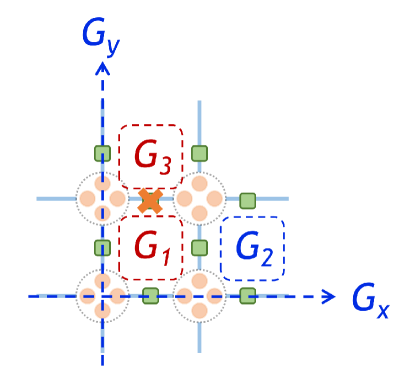
Figure 17: The on-site $\sigma_{z}$ operator creates a pair of visons when acting on the ground state with quantum number $\mathbf{q}=(+,+,+,+,+)$. The quantum number corresponding to the operators $G_{1}$ and $G_{3}$ is then changed, leading to an excited state with quantum number $\mathbf{q}^{\prime}=(+,+,-,+,-)$.

Furthermore, notice that the $\sigma_{z}$ operator does not commute with the gauge operator $G_{p}$. In fact, if we operate on the site with spin $\sigma_{z}^{1}$ with the gauge operator $G_{p}=\sigma_{x}^{1}\sigma_{x}^{2}\sigma_{x}^{3}\sigma_{x}^{4}$, the $\sigma_{z}$ operator changes the quantum number corresponding to $G_{p}$ since

$$\sigma_{z}^{1}G_{p}=-G_{p}\sigma_{z}^{1}.$$ (40)

As illustrated in Fig. 17, acting with a $\sigma_{z}$ operator on the ground state with quantum number set $\mathbf{q}=(+,+,+,+,+)$ creates a pair of visons and thereby changes the quantum numbers associated with $G_{1}$ and $G_{3}$, leading to a new quantum number set $\mathbf{q}^{\prime}=(+,+,-,+,-)$. This means that the ground state will have non-zero matrix elements only to the states with the right quantum number set. Thus, we can safely assume the matrix elements $|\sigma_{a0}^{zz}|^{2}=0$ for low levels. If we ignore these term in the summation we have

$$G(\tau,\beta)\sim\{e^{-\tau\Delta_{10}}+e^{-(\beta-\tau)\Delta_{10}}\}.$$ (41)

In our simulations, we evaluate this non-equal time correlator at various values of $\tau$ and extract the gap $\Delta_{10}$ by fitting the results to Eq. (41).

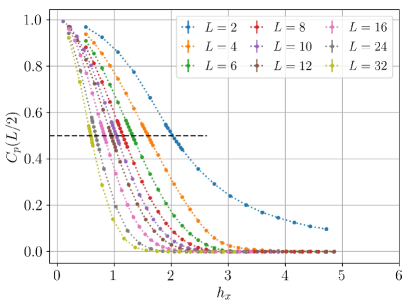
Figure 18: Wilson loop correlator calculated with SSE simulations of the square-lattice TFIM for several system sizes at inverse temperature $\beta=2L$. The inset shows the finite-size scaling of the location $h_{x}^{*}(L^{-1})$ for which the value of the correlator is $1/2$, as indicated by the horizontal dashed line. A power-law fit $y=a+bL^{-c}$ for the $L\geq 12$ data gives $a=-0.02(1)$, $b=3.15(2)$ and $c=0.472(7)$, indicating a vanishing value of the correlator at any transverse field in the thermodynamic limit.

Figure 19: Distribution $\rho(P_{x},P_{y})$ of the Wilson loop order parameter accumulated in SSE simulation at $\Gamma_{g}=0.2$ and three different values of the matter field; (a) $\Gamma_{m}=2.3952$ (in the $\mathbb{Z}_{2}$ QSL phase), (b) $\Gamma_{m}=2.4343$ (close to the transition point), and (c) $\Gamma_{m}=2.4563$ (in the confined phase). Near the transition point, in (b), five peaks are clearly observed, reflecting phase coexistence at a first-order transition.

Appendix D Parallel Wilson loop operator in square lattice transverse field Ising model

To show that the parallel Wilson loop operator does not detect the long range ferromagnetic phase, we perform simulations of the TFIM on $L\times L$ square lattices with periodic boundary conditions at inverse temperature $\beta=2L$. We compute the Wilson loop correlator defined in Eq. (20). As shown in Fig. 18, we draw the horizontal line at $C_{P}=1/2$ and extract the corresponding value $h_{x}^{*}(L)$ of the transverse field. In the inset of Fig. 18, we demonstrate finite-size scaling of the value $h_{x}^{*}$ as a function of $1/L$ with a power-law fit of the form $y=a+bL^{-c}$. Including data for the four largest system sizes, $L\geq 12$, we find the best fit with $a=-0.02(1)$, $b=3.15(2)$ and $c=0.472(7)$, confirming the expectation Wilson loop correlator vanishes for a conventional FM phase in the thermodynamic limit at any finite transverse field.

Appendix E Wilson loop order parameter distribution and phase coexistence

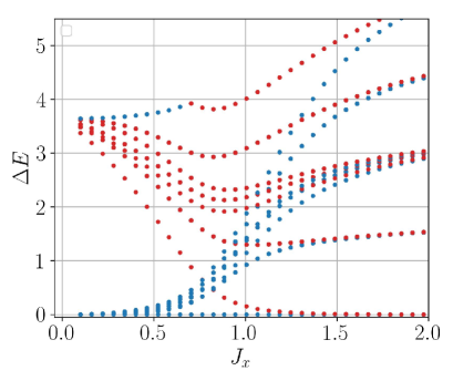
Figure 20: The low-energy levels previously shown in Fig. 15, now marked by the eigenvalues $\pm 1$ of the spin-inversion operator, Eq. (42), in model-XX at $\Gamma_{m}=1$. The gaps to the symmetric and antisymmetric states are marked with blue and red symbols, respectively. Out of all 64 states shown here, all the vison excitation states as well as the ground state are symmetric. The spinon excitations are all antisymmetric, except for the highest one, where a level crossing causes a change in symmetry at $J_{x}\approx 0.7$.

Here, we present simulation results for Wilson loop order parameter distribution $\rho(P_{x},P_{y})$ for model-X. The two components of the order parameter are defined as in Eq. (21). Fig. 19 shows color-coded plots of the distribution as the phase transition is traversed. Near the transition point, in Fig. 19(b), we observe a five-peak structure, indicating phase coexistence at a first-order transition. In (a) and (c) we observe distributions expected in systems with and without topological order, respectively.

Note that the four peaks at the corners in Fig. 19(a) and Fig. 19(b) should mathematically be of equal size, but they differ here because of the slow migration of the simulation between these peaks, which are separated by tunneling barriers in the SSE configuration space.

Appendix F Additional $\sigma_{x}$ spin inversion symmetry in model-XX

Model-XX possesses a spin inversion symmetry corresponding to the operator

$$V\equiv\prod_{i}\sigma_{i}^{z}\;,$$ (42)

which commutes with the Hamiltonian. In Fig. 20 we show the same energy levels of the model-XX at $\Gamma_{m}=1.0$ as previously in Fig. 15. Here different colors indicate symmetry or antisymmetry with respect to $V$. In the FM phase at large $J_{x}$ the gauge spins order along spin-$x$ direction, and the first excited state and the ground state are both from the block with topological quantum number set $\mathbf{q}=(+++++)$. In Fig. 15 we can observe how the symmetric and antisymmetric $V$ states become degenerate (strictly in the thermodynamic limit) to allow spontaneous symmetry breaking in the FM phase.

References

- Kitaev (2003) A. Kitaev, Ann. Phys. 303, 2 (2003).
- Moessner and Sondhi (2001) R. Moessner and S. L. Sondhi, Phys. Rev. Lett. 86, 1881 (2001).
- Misguich et al. (2002) G. Misguich, D. Serban, and V. Pasquier, Phys. Rev. Lett. 89, 137202 (2002).
- Balents et al. (2002) L. Balents, M. P. A. Fisher, and S. M. Girvin, Phys. Rev. B 65, 224412 (2002).
- Isakov et al. (2006) S. V. Isakov, Y. B. Kim, and A. Paramekanti, Phys. Rev. Lett. 97, 207204 (2006).
- Isakov et al. (2007) S. V. Isakov, A. Paramekanti, and Y. B. Kim, Phys. Rev. B 76, 224431 (2007).
- Chamon et al. (2020) C. Chamon, D. Green, and Z.-C. Yang, Phys. Rev. Lett. 125, 067203 (2020).
- Zhou et al. (2020) S. Zhou, D. Green, E. D. Dahl, and C. Chamon, “Experimental realization of spin liquids in a programmable quantum device,” (2020), arXiv:2009.07853 [cond-mat.str-el] .
- Wegner (1971) F. J. Wegner, J. Math. Phys. 12, 2259 (1971).
- Kogut (1979) J. B. Kogut, Rev. Mod. Phys. 51, 659 (1979).
- Rieger and Kawashima (1999) H. Rieger and N. Kawashima, Eur. Phys. J. B - Condensed Matter and Complex Systems 9, 233 (1999).
- du Croo de Jongh and van Leeuwen (1998) M. S. L. du Croo de Jongh and J. M. J. van Leeuwen, Phys. Rev. B 57, 8494 (1998).
- Liu et al. (2013) C.-W. Liu, A. Polkovnikov, and A. W. Sandvik, Phys. Rev. B 87, 174302 (2013).
- Fradkin (2013) E. Fradkin, Field Theories of Condensed Matter Physics, 2nd ed. (Cambridge University Press, 2013).
- You et al. (2007) W.-L. You, Y.-W. Li, and S.-J. Gu, Phys. Rev. E 76, 022101 (2007).
- Gu (2010) S.-J. Gu, Int. J. Mod. Phys. B 24, 4371 (2010).
- Prelovšek and Bonča (2013) P. Prelovšek and J. Bonča, “Ground state and finite temperature lanczos methods,” in Strongly Correlated Systems: Numerical Methods, edited by A. Avella and F. Mancini (Springer Berlin Heidelberg, Berlin, Heidelberg, 2013) pp. 1–30.
- Sandvik (2010) A. W. Sandvik, AIP Conf. Proc. 1297, 135 (2010).
- Sandvik (2019) A. W. Sandvik, “Stochastic series expansion methods,” in Many-Body Methods for Real Materials, Modeling and Simulation, Vol. 9, edited by E. K. Eva Pavarini and S. Zhang (Verlag des Forschungszentrum Julich, 2019).
- Wang et al. (2015) L. Wang, Y.-H. Liu, J. Imriška, P. N. Ma, and M. Troyer, Phys. Rev. X 5, 031007 (2015).
- Hukushima and Nemoto (1996) K. Hukushima and K. Nemoto, J. Phys. Soc. Jpn. 65, 1604 (1996).
- Hukushima et al. (1996) K. Hukushima, H. Takayama, and K. Nemoto, Int. J. Mod. Phys. C 07, 337 (1996).
- Sengupta et al. (2002) P. Sengupta, A. W. Sandvik, and D. K. Campbell, Phys. Rev. B 65, 155113 (2002).
- Fisher and Berker (1982) M. E. Fisher and A. N. Berker, Phys. Rev. B 26, 2507 (1982).
- Binder and Landau (1984) K. Binder and D. P. Landau, Phys. Rev. B 30, 1477 (1984).
- Sen and Sandvik (2010) A. Sen and A. W. Sandvik, Phys. Rev. B 82, 174428 (2010).
- Zhao et al. (2019) B. Zhao, P. Weinberg, and A. W. Sandvik, Nat. Phys. 15, 678 (2019).
- Elitzur (1975) S. Elitzur, Phys. Rev. D 12, 3978 (1975).
- Kotecký (1992) R. Kotecký, Astrophys. Space Sci. 193, 163 (1992).
- Xu et al. (2018) N. Xu, C. Castelnovo, R. G. Melko, C. Chamon, and A. W. Sandvik, Phys. Rev. B 97, 024432 (2018).
- Vollmayr et al. (1993) K. Vollmayr, J. D. Reger, M. Scheucher, and K. Binder, Z. Phys. B Condensed Matter 91, 113 (1993).
- Iino et al. (2019) S. Iino, S. Morita, N. Kawashima, and A. W. Sandvik, J. Phys. Soc. Jpn. 88, 034006 (2019).
- Hart et al. (2021) O. Hart, Y. Wan, and C. Castelnovo, Nat. Commun. 12 (2021).