Deconfinement of classical Yang-Mills color fields in a disorder potential

Abstract

We study numerically and analytically the behavior of classical Yang-Mills color fields in a random one-dimensional potential described by the Anderson model with disorder. Above a certain threshold the nonlinear interactions of Yang-Mills fields lead to chaos and deconfinement of color wavepackets with their subdiffusive spreading in space. The algebraic exponent of the second moment growth in time is found to be in a range of 0.3 to 0.4. Below the threshold color wavepackets remain confined even if a very slow spreading at very long times is not excluded due to subtle nonlinear effects and the Arnold diffusion for the case when initially color packets are located in a close vicinity. In a case of large initial separation of color wavepackets they remain well confined and localized in space. We also present comparison with the behavior of the one-component field model of discrete Anderson nonlinear Schrödinger equation with disorder.

I Introduction

The Yang-Mills (YM) gauge fields were introduced ym for an isotropic-invariant description of strong interactions. The investigation of properties of these fields still remains an interesting and important problem. The studies of classical YM fields are also important for applications in several problems of quantization polyakov1 ; polyakov2 . The classical dynamics of these fields is essentially nonlinear and nontrivial. Its analysis is rather important for semiclassical description of strong YM vacuum fluctuations polyakov3 ; polyakov4 ; vainstein ; shuryak2002 . Thus the investigation of nonlinear dynamics and time evolution of classical YM fields represents a relevant topic.

The important class of classical YM models was introduced in matinyan1 where the YM fields are homogeneous in space so that the time evolution is described only by nonlinear dynamics of interacting colors. In general this Hamiltonian dynamics of color YM fields was shown to be chaotic chis1 ; matinyan2 ; chis2 even if certain integrable solutions also exist. Thus the YM dynamics belongs to a generic class of chaotic Hamiltonian systems with divided phase space with small integrability islands embedded in a chaotic sea chirikov1979 ; lichtenberg . Even if important mathematical results have been obtained for chaotic dynamics (see e.g. arnold ; sinai ) the properties of chaos with such a divided phase space, composed of integrable islands surrounded by a chaotic component, still remain very difficult for mathematical analysis. The existence of chaos of classical homogeneous YM fields has been reported already some time ago matinyan1 ; matinyan2 ; chis1 ; chis2 but still these YM fields and related models attract attention of researchers (see e.g. ymclass1 ; ymclass2 ; ymclass3 ).

The above dynamics of YM color fields can be reduced to a rather simple Hamiltonian which for $N_{C}=2,3$ colors reads:

$$H=\sum^{N_{C}}_{i=1}({p_{\mu}}^{2}+m{x_{\mu}}^{2})/2+\beta\sum_{\mu^{\prime}\neq\mu}{x_{\mu^{\prime}}}^{2}{x_{\mu}}^{2}/2\;,$$ (1)

where $(p_{\mu},x_{\nu})$ are effective conjugated momentum and coordinate, color index is $\mu=1,...N_{C}$, $m$ is mass, which is zero or finite in presence of Higgs mechanism, and $\beta$ determines the strength of nonlinear interactions of colors matinyan1 ; chis1 ; matinyan2 ; chis2 . An interesting feature of the finite mass case (e.g. $m=1$ in dimensionless units used here) is that the measure of chaos remains finite and large (about $50\%$) even in the limit of very weak nonlinearity $\beta\rightarrow 0$ since the Kolmogorov-Arnold-Moser (KAM) theorem lichtenberg is not valid when all color masses (or oscillator frequencies) are the same chis2 .

Till present the classical dynamics of YM colors was analyzed for fields homogeneous in space. Here we consider the case of space nonhomogeneous fields. Namely, we study a spreading of such YM fields in space in presence of disorder potential which corresponds to another generic limiting case of space properties. Such a disorder corresponds to random properties of vacuum in Quantum Chromodynamics (QCD) discussed in the literature (see e.g. shuryak1980 ; olesen ; kirzhnits ; shuryak1993 ). It is well known that in quantum mechanics a disorder potential may lead to a localization of probability spreading due to quantum interference effects. This phenomenon is known as the Anderson localization anderson and plays an important role for electron transport in solid-state systems with disorder imry ; montambaux ; mirlin . The eigenstates of such a system are exponentially localized in 1 and 2 dimensions (1D and 2D) while in 3 dimensions (3D) a delocalization transition takes place at a disorder below certain threshold (see e.g. review mirlin ).

The effects on nonlinearity on Anderson localization in 1D lattice were investigated in dls1993 where it was shown that the localization is preserved at weak nonlinearity while above a certain threshold a subdiffusive spreading over the whole lattice takes place. The detailed numerical studies of this phenomenon in Disordered Anderson Nonlinear Schrödinger Equation (DANSE) have been reported in molina ; dls2008 ; flach2009 and results of different groups were reviewed in mulansky ; flach . The subdiffusive spreading has been studied for various nonlinear models in 1D and 2D (see e.g. garcia ; flachkg ; ermann ; flach2019 ; skokos ) with a spreading continuing up to enormously long dimensional times $t\sim 2\times 10^{12}$ reported for a 1D model in flach2019 . The interest to the effects of nonlinearity on Anderson localization is also supported by related experimental studies of wave propagation in a disordered nonlinear media segev ; lahini and spreading of Bose-Einstein cold atom condensates in optical disorder lattices inguscio1 ; inguscio2 described by the Gross-Pitaevskii equation.

All above investigations of packet spreading in a disorder potential with nonlinearity have been done for one-component nonlinear field of DANSE with nonlinear self-interaction (see e.g. dls2008 ; mulansky ; flach ). The case of YM color dynamics is different since nonlinearity appears only due to interactions of color components. In fact possible implications of randomness, dynamical chaos, Anderson localization and confinement has been discussed in olesen ; kirzhnits . The deconfinement transition in QCD at finite temperature is also under active investigation (see e.g. deconf1 ; deconf2 ; deconf3 and Refs. therein). Here, we find that under certain conditions the nonlinear interaction of YM colors leads to deconfinement of YM fields and their unlimited subdiffusive spreading in space. In the case of weak nonlinearity or spacial separation of YM color components the Anderson localization is preserved and fields remain localized in space. We hope that the obtained results may be of interest for the deconfinement phenomenon of quantum YM fields which attracts a significant interest.

The paper is organized as follows: in Section II, we give the system description, the numerical and analytical results are given in Section III, discussion of results is given in Section IV.

II Model description

II.1 DANSE

Me start with a brief description of DANSE model studied in dls2008 ; mulansky ; flach ; garcia . The wavefunction evolution of DANSE is described by the equation:

$$i\hbar{{\partial{\psi}_{n}}\over{\partial{t}}}=E_{n}{\psi}_{n}+{\beta}{\mid{\psi_{n}}\mid}^{2}\psi_{n}+V({\psi_{n+1}}+{\psi_{n-1})}\;.$$ (2)

Here $\beta$ determines nonlinearity strength, $V$ gives near-neighboring hopping matrix element, on-site disorder energies are randomly distributed in the range $-W/2<E_{n}<W/2$, and the total probability is conserved and normalized to unity $\sum_{n}{\mid{\psi_{n}}\mid}^{2}=1$. For $\beta=0$ all eigenstates are exponentially localized with $|\psi|\propto\exp(-|n-n_{0}|/\ell)$ and localization length is $\ell\approx 96(V/W)^{2}$ at the energy band center and weak disorder kramer1993 . Here $n_{0}$ marks a center of wavefunction. We consider a case of relatively weak disorder with $\ell>1$. For convenience we set $\hbar=V=1$ so that the energy coincides with the frequency.

Above a certain threshold $\beta>\beta_{c}$ the nonlinearity leads to a destruction of localization with a subdiffusive spreading of wavepacket width $\Delta n=n-n_{0}$:

$$\sigma=<(\Delta n)^{2}>\propto t^{\alpha}\;,$$ (3)

where brackets mark averaging over wavefunction at time $t$ and $\alpha$ is the subdiffusion exponent. The numerical simulations give its value being in a range $0.3\leq\alpha\leq 0.4$. Certain analytical arguments were given for values $\alpha=0.4$ dls1993 ; dls2008 ; garcia and $\alpha=1/3$ flach . An introduction of randomness in eigenstate phases of linear problem is supposed to produce a spreading with $\alpha=0.5$ basko ; flach . Indeed, an increase of dephasing leads to a growth of $\alpha$ approaching the value $\alpha=0.5$ ermann .

It is difficult to give an exact estimate of the threshold value $\beta_{c}$. The numerical results show that at $\beta=0.1;0.03$ the wavepacket square width $\sigma$ remains bounded without significant increase up to times $t=10^{8}$ dls2008 . However, it is possible that some type of Arnold diffusion along tiny chaotic layers chirikov1979 ; lichtenberg ; chivech may lead to a very slow spreading of a very small wavepacket fraction. It should be pointed that the Anderson localization is characterized by a pure-point dense spectrum and its perturbation by nonlinearity represents a very difficult problem for mathematical analysis. A reader can find some mathematical results for this problem reported in fishman ; wang .

A surprising feature of unlimited spreading at $\beta>\beta_{c}$ is that with growth of $\Delta n$ the relative local contribution of nonlinear term in (2) decreases as $\beta|\psi|^{2}\sim\beta/\Delta n\propto\beta/t^{\alpha/2}$ and on a first glance it seems that nonlinearity becomes weaker and weaker with time. In dls1993 is was argued that even being small this term gives a local nonlinear frequency spreading $\delta\omega\sim\beta/\Delta n$ which at $\beta>\beta_{c}\sim 1$ remains larger than the typical spacing $\Delta\omega\sim 1/\Delta n$ between frequencies of linear eigenmodes populated due to subdiffusive spreading of wavepacket at time $t$. As soon as $\delta\omega>\Delta\omega$ the spectrum of motion remains continuous and thus the spreading can continue unlimitedly in time. However, a better understanding of origins of such unlimited spreading is still highly desirable.

II.2 YM color models

In a similarity with dynamics of homogeneous YM fields described by Hamiltonian (1) and DANSE (2) we model the dynamics of YM color fields in a disorder potential by the nonlinear Schrödinger equation:

$$i{\partial{\psi^{\mu}_{n}}\over{\partial{t}}}=E_{n}\psi^{\mu}_{n}+{\beta}({\sum_{\mu^{\prime}\neq\mu}\mid{\psi^{\mu^{\prime}}_{n}}\mid}^{2})\psi^{\mu}_{n}+({\psi^{\mu}_{n+1}}+{\psi^{\mu}_{n-1})}\;.$$ (4)

Here $\mu=1,...,N_{C}$ is color index changing from $1$ to $2$ for two YM colors $N_{C}=2$ or from $1$ to $3$ for three colors $N_{C}=3$. We denote these two cases as $YMCA2$ and $YMCA3$ respectively (with A for agent). At zero nonlinearity $\beta=0$ each color evolution is described by 1D Anderson model with the same disorder $E_{n}$ for all colors and being the same as in (2). In absence of hopping to nearby sites and all energies $E_{n}$ being equal we have the dynamics of color fields described by equations similar to those for the homogeneous YM fields from Hamiltonian (1). Thus we consider the equations (4) as a realistic model of evolution of classical YM color fields in a disorder potential.

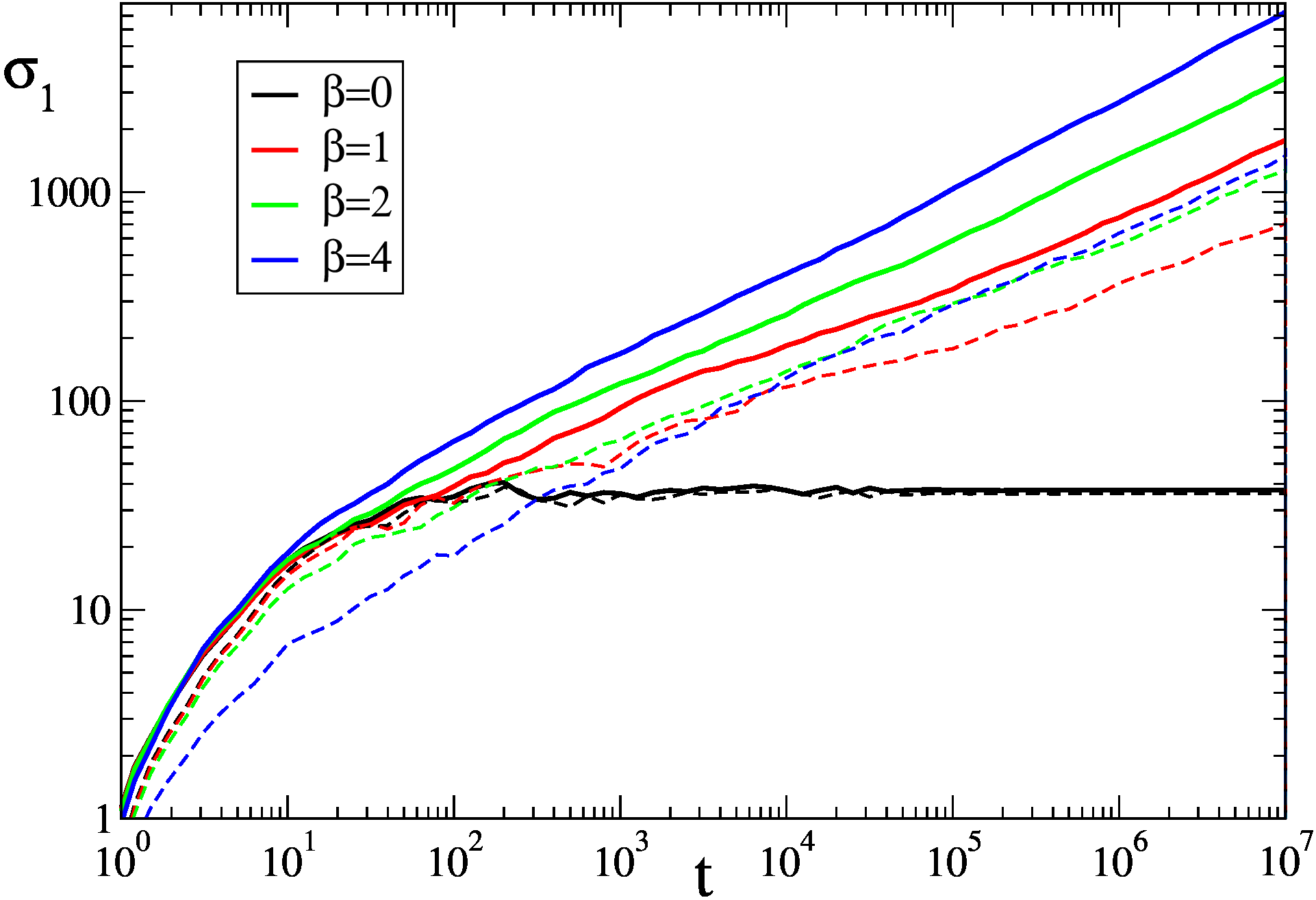
Figure 1: Time evolution of the second moment $\sigma_{1}$ of probability distribution, defined in the text, for YMCA3 model with 3 colors (4) (solid curves) and DANSE model (2) (dashed curves) at $\beta=0$ (black curves), $\beta=1$ (red curves), $\beta=2$ (green curves) and $\beta=4$ (blue curves) at $W=4$. At initial time the 3 color packets are located at 3 different sites $n=-1,0,1$ for YMCA3; for DANSE initial probability is at $n=0$. The average is done over 20 random realizations of disorder and over logarithmic equidistant intervals of time.

As for DANSE, the evolution of YM fields (4) has the energy conservation, also the probability is conserved for each component normalized to unity $\sum_{n}\mid{\psi^{\mu}_{n}}\mid^{2}=1$. The numerical simulations of DANSE and Klein-Gordon nonlinear (KGN) model with disorder flach ; flachkg ; ermannnjp show that the exponent $\alpha$ is approximately the same in these two models even if only energy is conserved in the KGN case. Thus we also expect that the probability conservation for each color component will not affect the spreading exponent $\alpha$. Indeed, the number of degrees of freedom in (4) is given by number of lattice sites multiplied by $N_{C}$ being much larger than the number of integrals $N_{C}+1$ of energy and component probabilities.

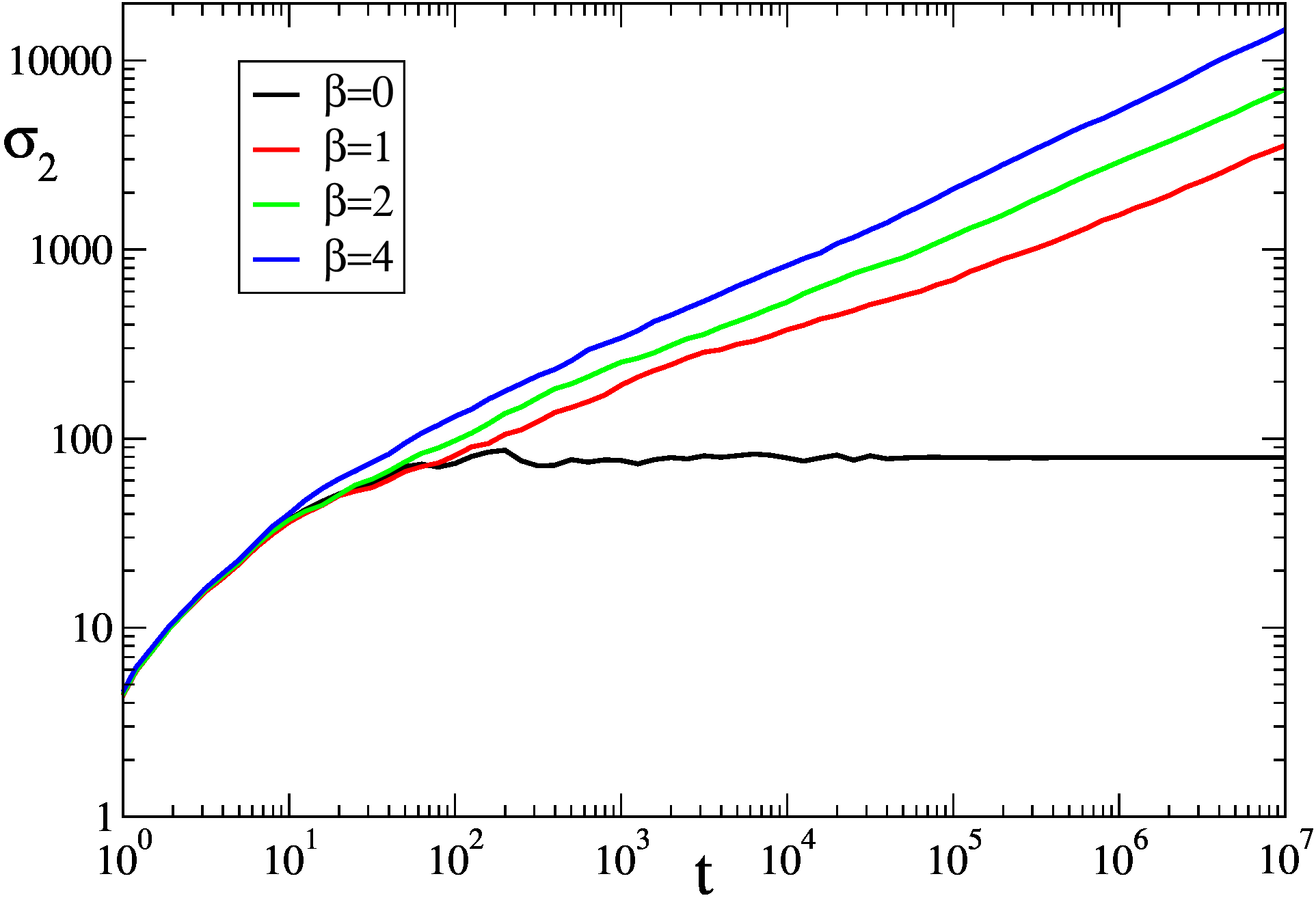
Figure 2: Same as in Fig. 1 but for the second moment $\sigma_{2}$ of probability distribution for YMCA3 model, defined in the text.

From the structure of YM equations (4) we can make certain direct observations. At first, it is possible to consider the symmetric case when initially all color components $\psi^{\mu}_{n}$ are the same. Then their evolution is described by the DANSE equation (2) with some rescaling of $\beta$ for $N_{C}=3$. However, since the field evolution is chaotic this solution is unstable and small corrections to this symmetric state grow exponentially with time so that this symmetry is completely destroyed very rapidly. Still such a symmetric case allows to expect that the spreading exponent $\alpha$ will have a value similar to those found for DANSE. As for DANSE we expect that YM fields remain confined or localized below a certain chaos threshold with $\beta\ll\beta_{c}\sim 1$. In spite of this possible similarity between DANSE and YMCA models there are two important differences between them. Thus if initially color wavepackets are located far from each other with a typical distance between them $R_{C}$ being significantly larger than the localization length $\ell$ of the linear case ($R_{c}\gg\ell$) then an effective interaction between colors becomes exponentially small $\beta_{eff}\propto\beta\exp(-2R_{C}/\ell)$ so that we have $\beta_{eff}\ll\beta_{c}\sim 1$. Thus we expect that such initial states will remain exponentially localized or confined for all times. Another new element of YMCA, compared to DANSE case, is that the eigenenergies $\varepsilon_{m}$ of linear problem eigenmodes at $\beta=0$ are the same for all colors. Thus for one site and 3 colors we have a dynamics being very similar to those of Higgs case with finite mass (1) studied in detail in chis2 . Due to this degeneracy the KAM theorem cannot be applied to this system and the measure of chaos remains about 50% even in the limit of nonlinearity going to zero chis2 . However, the initial wavepackets of colors should populate the same linear eigenmodes (this requires $R_{C}<\ell$). Such situation also generally appears in other type on nonlinear systems with many degrees of freedom mulansky2 . Since in YMCA at $N_{C}=3$ (4) there many eigenenergies $\varepsilon_{m}$ (linear frequencies) which are the same we expect that there are many initial configurations when colors are initially located on a distance $R_{c}\sim\ell$ and their dynamics remains chaotic even for very small nonlinearity $\beta\rightarrow 0$. However, a question about spreading of such chaos over lattice sites remains open.

III Numerical results for time evolution of YM colors

Following the approach used in dls2008 , the numerical integration of Eqs. (2), (4) is done by the Trotter decomposition with a time step $\Delta t=0.05$ and the total number of sites $N=1001$ for each color with the fast Fourier transform from coordinate to momentum representation and back. This integration scheme is symplectic and conserves probability exactly. Its efficiency has been confirmed by various numerical simulations (see e.g. dls2008 ; mulansky ; flach ; garcia ). We checked that the variation of system size $N$ and integration time step $\Delta t$ does not affect the results. We present here the results mainly for a typical disorder strength $W=4$ and nonlinearity values $\beta=0,1,2,4$. The spreading of color probabilities is characterized by the squared wavepacket width at different times defined as: $\sigma_{1}=\langle n_{1}^{2}\rangle-\langle n_{1}\rangle^{2}$ for DANSE, $\sigma_{1}=\sum^{N_{C}}_{\mu=1}\left(\langle n_{\mu}^{2}\rangle-\langle n_{\mu}\rangle^{2}\rangle\right)/N_{C}$ for YMCA2, YMCA3 and relative square moments $\sigma_{2}=\left\langle(n_{1}-n_{2})^{2}\right\rangle$ for YMCA2 and $\sigma_{2}=\left[\left\langle(n_{1}-n_{2})^{2}\right\rangle+\left\langle(n_{1}-n_{3})^{2}\right\rangle+\left\langle(n_{2}-n_{3})^{2}\right\rangle\right]/3$ for YMCA3. Here brackets mark the average over wavefunction. The results are also averaged over 20 disorder realisations.

III.1 Deconfinement and subdiffusive spreading of YM colors

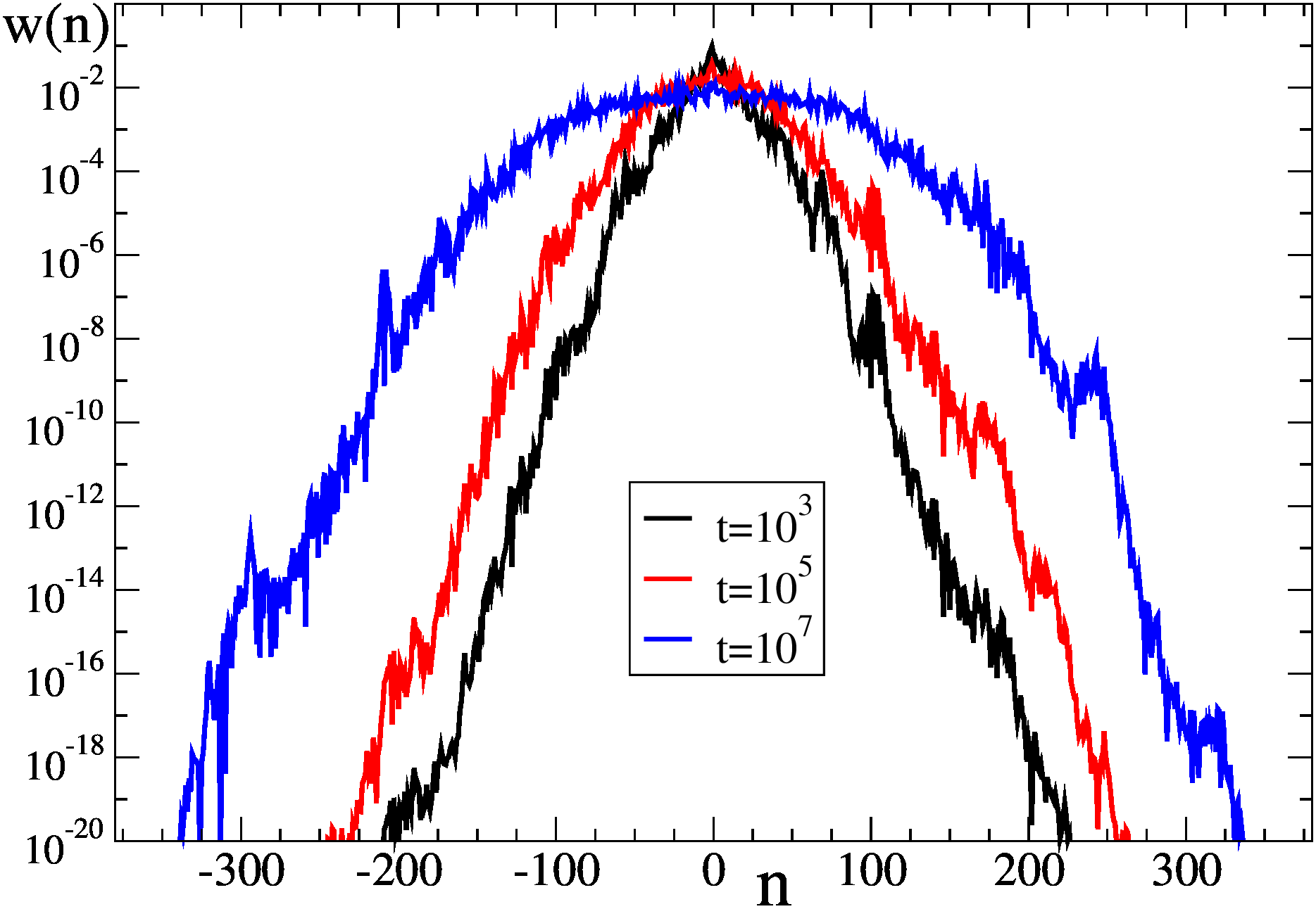
Figure 3: Probability distributions $w(n)=\sum_{\mu=1}^{N_{C}}\mid{\psi^{\mu}_{n}}\mid^{2}/N_{C}$ for YMCA3 model ($N_{C}=3$, $\beta=2$, $W=4$) are shown at times $t=10^{3}$ (black curve), $t=10^{5}$ (red curve) and $t=10^{7}$ (blue curve); probabilities are averaged over 20 disorder realizations.

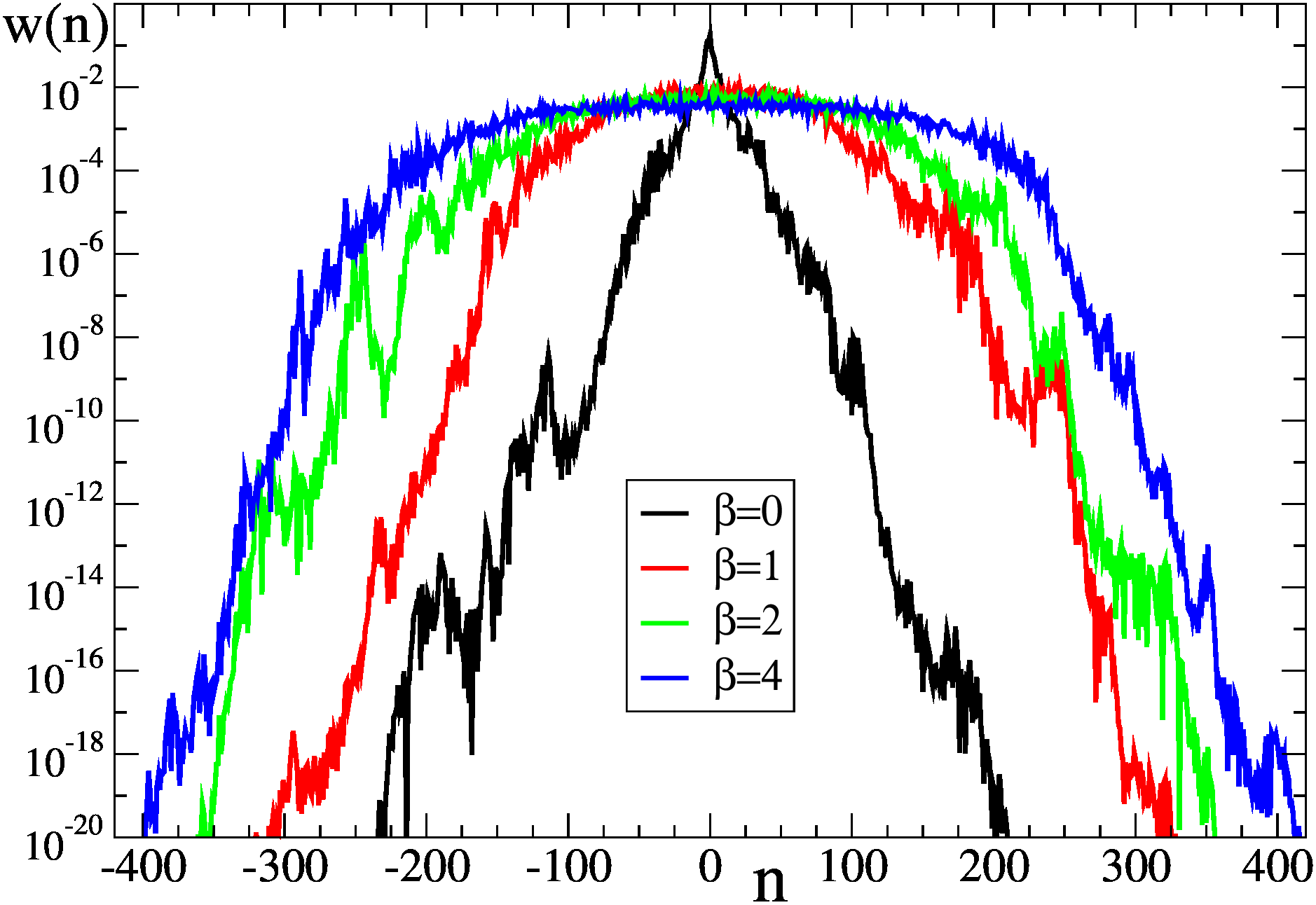
Figure 4: Same as in Fig. 3 but all distributions $w(n)$ of YMCA3 are shown at time $t=10^{7}$ for $\beta=0$ (black curve), $\beta=1$ (red curve), $\beta=2$ (green curve) and $\beta=4$ (blue curve); probabilities are averaged over 20 disorder realizations.

The time dependence of second moments $\sigma_{1}$ for DANSE and YMCA3 models is shown in Fig. 1 for different values of $\beta$ and disorder $W=4$. At such a disorder and $\beta=0$ the wavepacket spreads on approximately $\Delta n\approx 7$ sites in agreement with the theoretical value of the localization length $\ell=96/W^{2}=6$. In presence of nonlinear interactions there is a subdiffusive spreading of wavepacket which is somewhat stronger for YMCA3 compared to DANSE case. The time evolution of the second moment $\sigma_{2}$ for YMCA3 case is shown in Fig. 2 for the same values of $\beta$ as in Fig. 1. The growth of both moments $\sigma_{1}$ and $\sigma_{2}$ is very similar. This means that the color packets spread in such a way that they remain close to each other so that their effective interactions allow to make correlated joint transitions over localized eigenstates of the Anderson model at $\beta=0$. It is clear that interactions of colors leads to deconfinement of YM fields with the unlimited subdiffusive spreading over the whole lattice. The growth of moments $\sigma_{1},\sigma_{2}$ for YMCA2 case is very similar to those of YMCA3 and we do not show it here (but the obtained spearing exponents $\alpha$ are discussed below for both cases).

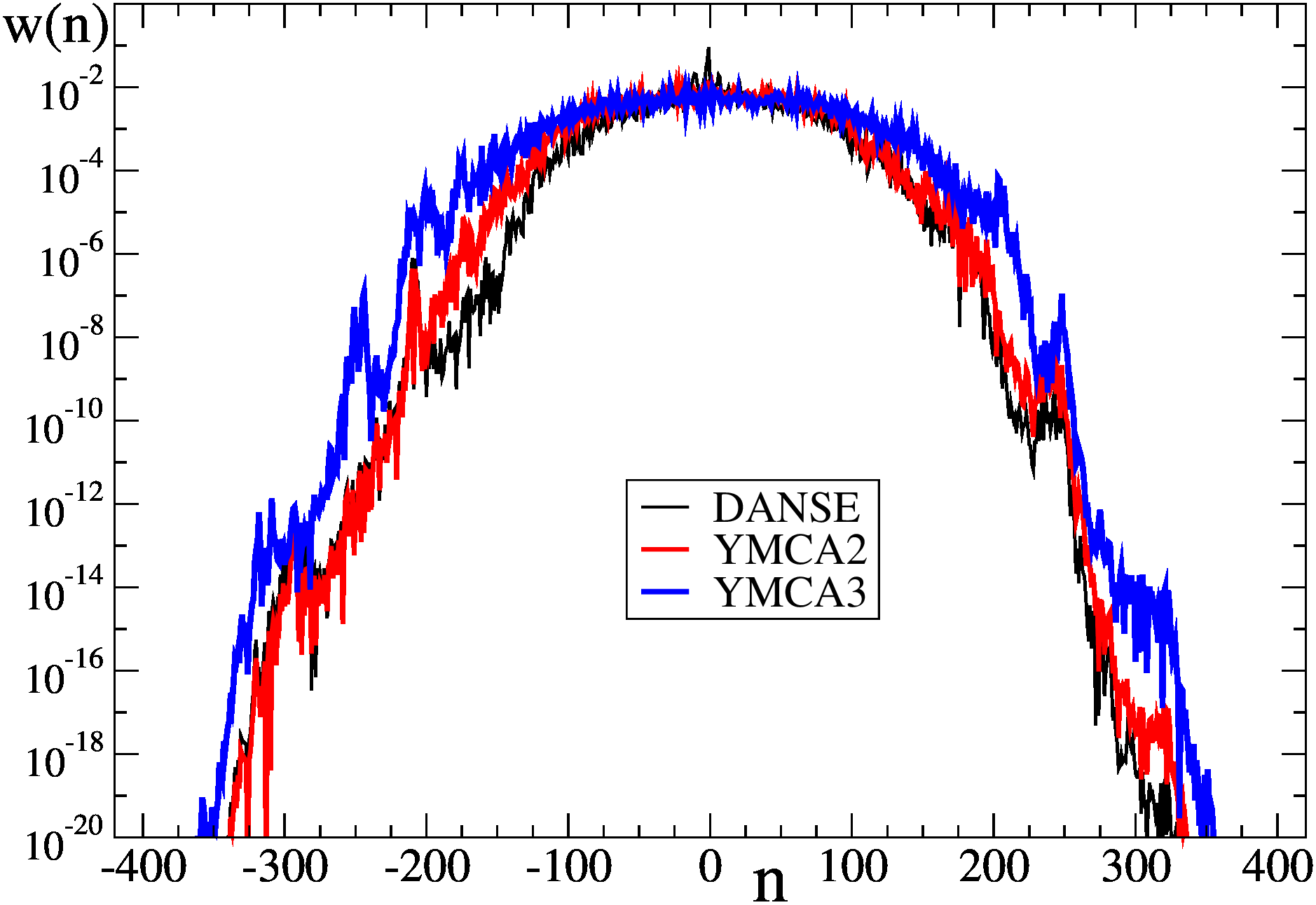
Figure 5: Probability distributions $w(n)$ are shown for DANSE (black curve), YMCA2 (red curve) and YMCA3 (blue curve) at $\beta=2,W=4$ and $t=10^{7}$; probabilities are averaged over 20 disorder realizations.

In Fig. 3 we show directly the probability distribution over lattice sites $w(n)=\sum_{\mu=1}^{N_{C}}\mid{\psi^{\mu}_{n}}\mid^{2}/N_{C}$ at different moments of time for YMCA3 case with $\beta=2$. There is a formation of quasi-plateau distribution which size $\Delta n$ increases with time. Outside of plateau there are probability tails which drop exponentially with the site number that corresponds to exponentially localized Anderson modes of linear problem.

The distributions $w(n)$ at largest reached time $t=10^{7}$ and different values of nonlinearity $\beta$ are shown in Fig. 4 The width of the above quasi-plateau size $\Delta n$ increases with $\beta$ being approximately $\Delta n\approx 220,320,440$ for $\beta=1,2,4$ respectively. These $\Delta n$ values are much larger than the Anderson localization length $\ell\approx 6$. Also the corresponding nonlinear frequency width $\Delta\omega\sim 1/\Delta n\ll 1/\ell$ becomes significantly smaller than a typical frequency spacing between modes inside localization length $\ell$. Due to these reasons we can argue that the numerical results show an asymptotic spearing of wavepacket of YM colors.

	$\alpha$
$\beta$	DANSE	YMCA2	YMCA3
1	$0.26\pm 0.02$	$0.297\pm 0.020$	$0.316\pm 0.010$
2	$0.317\pm 0.010$	$0.327\pm 0.020$	$0.363\pm 0.010$
4	$0.371\pm 0.020$	$0.378\pm 0.020$	$0.406\pm 0.010$

Table 1: Exponent $\alpha$ of growth of second moments $\sigma_{1,2}\propto t^{\alpha}$ for DANSE, YMCA2, YMCA3 models at different values of nonlinearity $\beta$ at $W=4$; the values of exponent are obtained by a fit in the time interval $2\leq\log_{10}t\leq 7$ for data averaged over 20 disorder realisations; initial states have colors located close to each other with $R_{C}=1$.

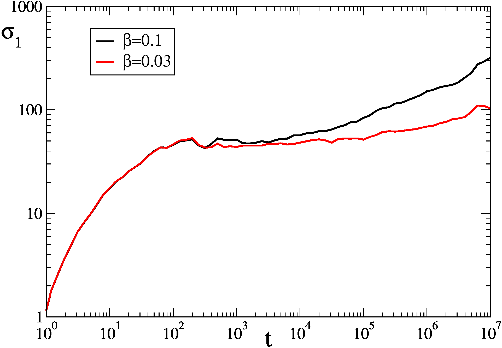
Figure 6: Time evolution of the second moment $\sigma_{1}$ of probability distribution, defined in the text, for YMCA3 model with 3 colors for $\beta=0.1$ (black curve), $\beta=0.03$ (red curve) at $W=4$. At initial time the 3 color packets are located at 3 different sites $n=-1,0,1$. The results are shown for 10 disorder realizations and logarithmic equidistant intervals of time.

The comparison of probability distributions for DANSE, YMCA2, YMCA3 models is shown in Fig. 5 for fixed $\beta,W$ and $t=10^{7}$. The most broad spreading corresponds to YMCA3 case. This is in a qualitative agreement with an expectation that, similar to Hamiltonian (1), there is an exact degeneracy of linear color eigenmodes modes so that here chaos is present even in the limit of very small $\beta$ similar to the situation discussed in chis2 ; mulansky2 (of course, this assumes that initial state have a close location of 3 colors so that degenerate linear modes are well populated, see discussion below).

According to the results of Figs. 1, 2 the growth of $\sigma_{1},\sigma_{2}$ at large times is well described by an algebraic function of time with the exponent $\alpha$. The values of $\alpha$, obtained from the fit for time range $100\leq t\leq 10^{7}$ are given in Table 1 for DANSE, YMCA2, YMCA3 models. For DANSE at $\beta=1$ the obtained value of $\alpha$ is a bit smaller than the one reported at dls2008 with $\alpha=0.306\pm 0.002$. We attribute this difference to a different number of realisations and longer time range used in dls2008 . We also should note that the spreading is rather slow in time and thus very long time simulations and large number of realizations are required to obtain accurate values of $\alpha$. Formal statistical errors reported here and in dls2008 are relatively small but the contribution of certain systematic effects, related to slow transitions between localized linear modes, may give more significant corrections to formal statistically averaged $\alpha$ values. From Table 1 we see a moderate increase of $\alpha$ for higher $\beta$ values. We also find that YMCA3 and YMCA2 models have a moderately higher values of $\alpha$ compared to DANSE case. We attribute this to a stronger chaos for YM colors compared to DANSE. Indeed, YM colors have additional color degrees of freedom that are supposed to generate a stronger chaos thus facilitating deconfinement and spreading of YM fields. However, due to the above points related to a slow spreading process further more advanced studies are required to firmly state if $\alpha$ is independent, or not, of $\beta,W$ and number of colors $N_{C}$.

III.2 Confinement and localization of YM colors

Above we discussed the cases with moderate strength of interactions of colors given by $\beta$. It is natural to expect that at small $\beta\ll\beta_{c}\sim 1$ the Anderson localization is preserved and fields remain localized in space. Indeed, the numerical results reported for DANSE dls2008 indicate that localization is preserved at small $\beta=0.1;0.03$. At the same time we note that in this limit the effects of slow processes like the Arnold diffusion chirikov1979 ; chivech are still possible with a very slow spreading of very small fraction of probability via tiny chaotic layers. The mathematical results are not able to clarify the behavior in this regime (see e.g. fishman ; wang ).

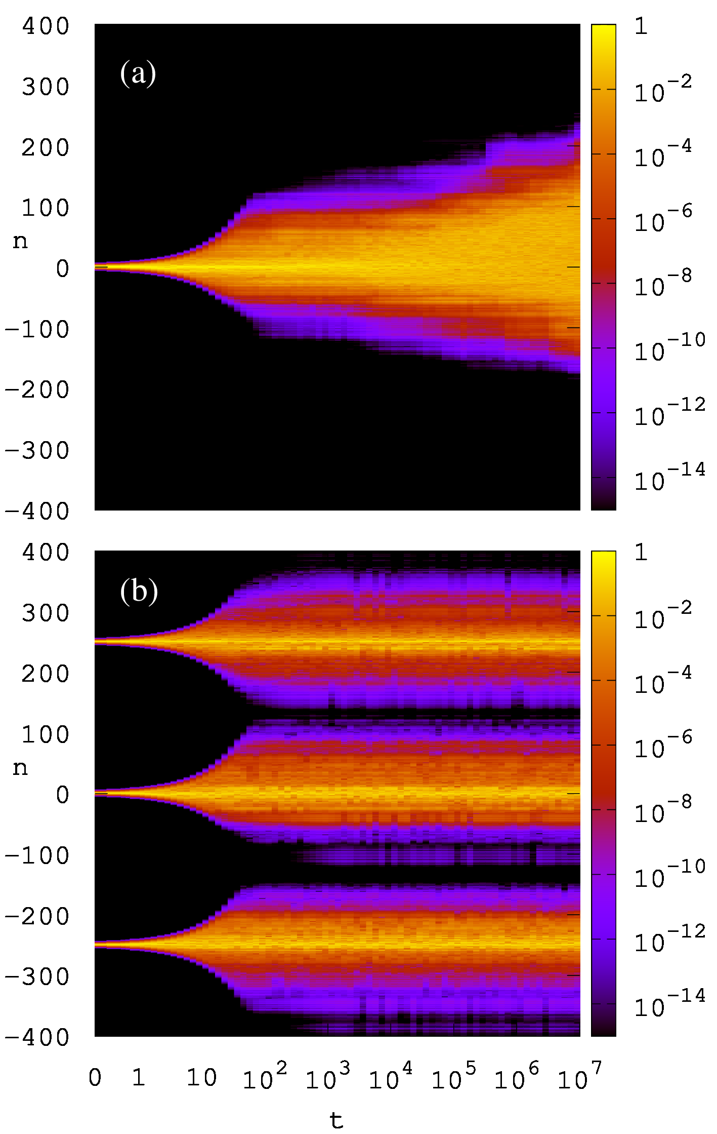
Figure 7: Probability distribution as a function of time $t$ for YMCA3 model at $\beta=2$, $W=4$, initial positions of 3 colors are $n=-1,0,1$ with $R_{C}=1$ (a); $n=-250,0,250$ with $R_{C}=250$ (b) for one disorder realisation; color bar shows probability $w(n)$ of YM color fields.

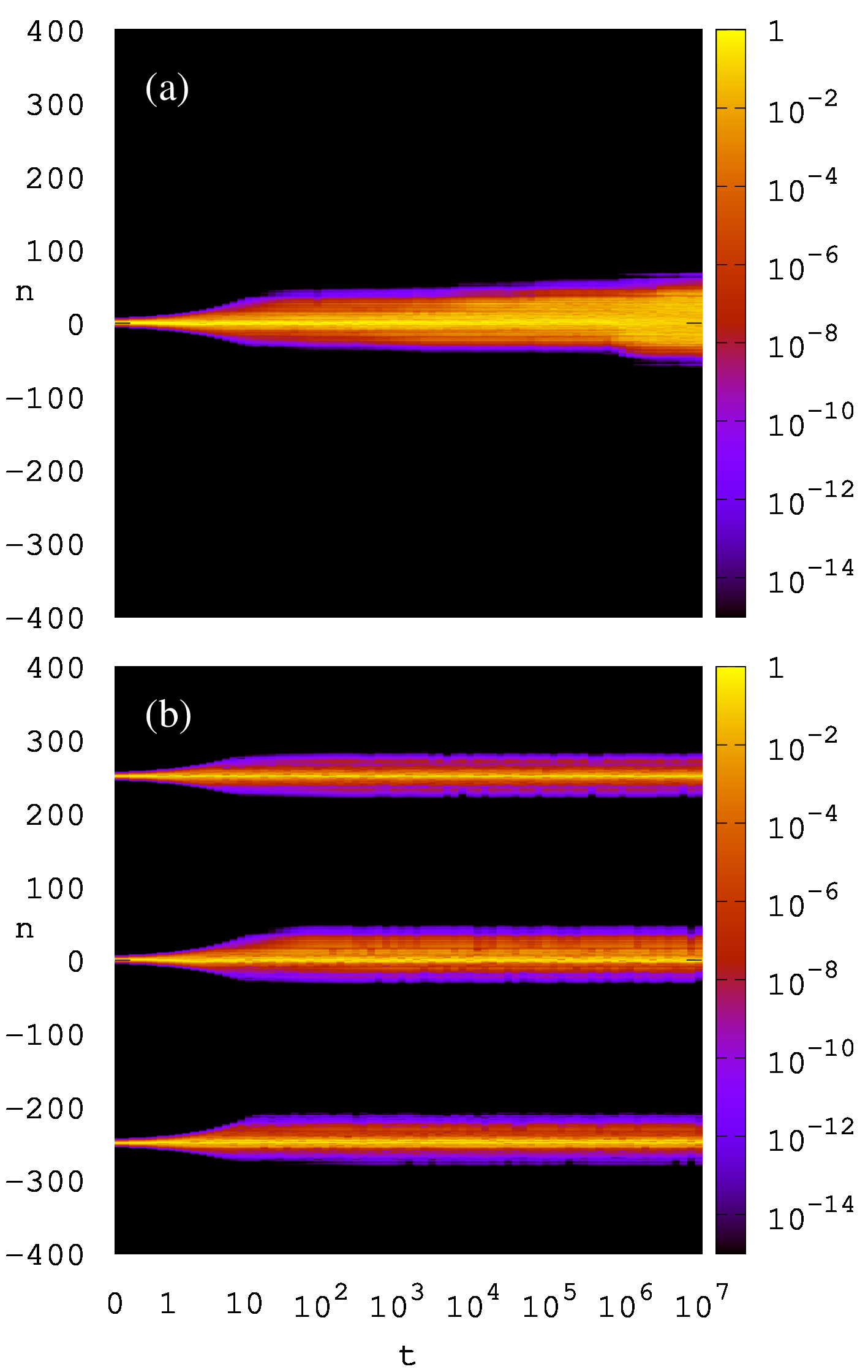
Figure 8: Same as in Fig. 7 but for $W=8$.

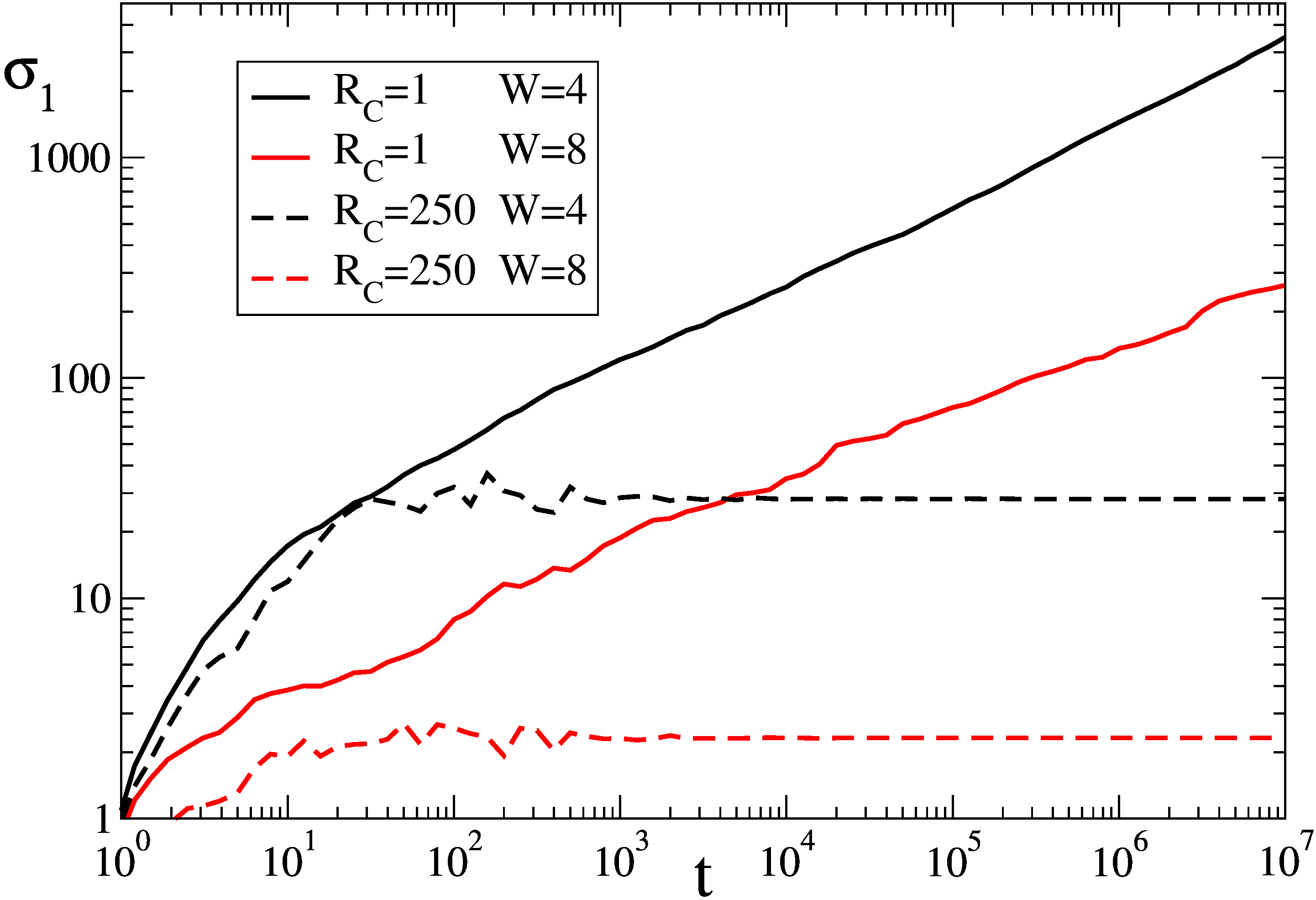
Figure 9: Time dependence of $\sigma_{1}(t)$ for YMCA3 at $\beta=2$ for initial distance between color positions: $R_{C}=1$ (full black curve for 20 disorder realisations at $W=4$ same as in Fig. 1); $R_{C}=250$ (dashed black curve for one disorder realisation at $W=4$ same as in Fig. 7); $R_{C}=1$ (full red curve for 10 disorder realisations at $W=8$); $R_{C}=250$ (dashed red curve for one disorder realisation at $W=8$ same as in Fig. 8).

For YMCA3 case at such small values of nonlinearity $\beta=0.1;0.03$ we show the time dependence of second moment $\sigma_{1}$ in Fig. 6 Here the second moment $\sigma_{1}$ remains substantially smaller compared to $\beta=1,2,4$ cases shown in Fig. 1. However, a slow increase of $\sigma_{1}$ at very large times $t>10^{5}$ is not excluded. We attribute this to a degeneracy of linear eigenmodes which, similar to the case of YMCA3 Hamiltonian (1), leads to a high fraction of chaotic phase space even for $\beta\rightarrow 0$, as discussed in chis2 ; mulansky2 for 3 colors (we note that for Hamiltonian with 2 colors (1) there is no chaos in the limit of small $\beta$ but only a significant energy exchange between two colors chis2 ). Thus, a slow spreading at very large times for YMCA3 case may take place due to frequency degeneracy present for color fields initially located on a distance $R_{C}<\ell$. The effect of very slow Arnold diffusion chirikov1979 ; chivech can be also present for a small fraction of global probability.

The interesting point is that the above exact frequency degeneracy is present only if initial color packets are close to each other. In the opposite case with their initial significant separation on a distance $R_{C}\gg\ell$ the effective nonlinear interactions between colors drop exponentially with $R_{C}$ due to localization of linear eigenmodes. In addition the frequencies of eigenmodes populated for such packets with large separation $R_{C}\gg\ell$ and statistically different and have no exact degeneracy in contrast to the case with $R_{C}<\ell$. Thus for $R_{C}\gg\ell$ we argue that this case corresponds to a very small effective interactions with $\beta_{eff}\propto\beta\exp(-2R_{C}/\ell)\ll 1$ and that the color YM fields remain confined and localized. This is confirmed by the results shown in Figs. 7, 8 were we compare close and distant location of initial color packets. We have clear deconfinement and spreading for $R_{C}=1$ (for $W=8$, $\beta=2$, $R_{c}=1$ the fit gives $\alpha=0.30\pm 0.02$ being smaller than the value at $W=4$ in Table 1). In contrast, for $R_{C}\gg\ell$ there is confinement and localization of YM color fields. The increase of disorder strength from $W=4$ in Fig. 7 to $W=8$ in Fig. 8 gives at $R_{C}=250$ a strong enhancement of localization of color YM fields. For distant initial positions of color fields $R_{C}=250$ the second moment $\sigma_{1}(t)$ shows absolutely no growth with time as it is shown in Fig. 9.

It is interesting to note that the situation with localization-delocalization of color YM fields reminds those of a quantum problem of two interacting particles coherently propagating in a disorder potential and being localized if separated by a distance being larger than a one-particle localization length (see e.g. dlstip ; imrytip ; frahmtip ).

III.3 Simple estimates for spreading exponent of YM colors

Here we present simple estimates for the spreading exponent $\alpha$ of the second moment growth $\sigma_{1,2}\propto t^{\alpha}$. Following the approach described in dls1993 ; garcia it is useful to rewrite Eq. (4) in the basis of eigenstates of the linear system at $\beta=0$. The transformation from lattice representation to eigenstate basis reads $\psi^{\mu}_{n}=\sum_{m}Q^{\mu}_{nm}C^{\mu}_{m}$ for each color $\mu$. Then the time evolution Eq. (4) takes the form:

$$i{{\partial C^{\mu}_{m}}\over{\partial{t}}}=\epsilon_{m}C^{\mu}_{m}+\beta\sum_{\mu^{\prime}\neq\mu}\sum_{{m_{1}}{m_{2}}{m_{3}}}U^{\mu^{\prime}}_{{m}{m_{1}}{m_{2}}{m_{3}}}C^{\mu}_{m_{1}}C^{{\mu^{\prime}}*}_{m_{2}}C^{\mu^{\prime}}_{m_{3}}$$ (5)

where $\epsilon_{m}$ are the eigenenergies of linear system being the same for all colors. The transitions between linear eigenmodes take place only due to the nonlinear $\beta$-term with the transition matrix elements $U^{\mu^{\prime}}_{mm_{1}m_{2}m_{3}}=\sum_{n}(Q^{{\mu}}_{nm})^{-1}Q^{\mu^{\prime}}_{nm_{1}}(Q^{\mu^{\prime}}_{nm_{2}})^{*}Q^{\mu}_{nm_{3}}$. Due to the exponential localization of linear eigenstates the sum over each $m$-index in (5) contains about $\ell$ terms.

In dls1993 it was argued that in the assumption that there is a plateau of size $\Delta n$ with random coefficients of approximately equal amplitudes and random signs or phases and zero amplitudes outside the plateau. Then the population of states outside of plateau should go with the rate $\Gamma\sim|C|^{6}\sim 1/(\Delta n)^{3}$ on nearby sites on a distance $\ell$. This gives a diffusion rate $D\sim\ell^{2}\Gamma\sim\ell^{2}/(\Delta n)^{3}\sim(\Delta n)^{2}/t$ leading to the growth $(\Delta n)^{2}\sim\sigma_{1,2}\sim t^{\alpha}$ with the spreading exponent $\alpha=2/5$.

There are also other type of arguments leading to the same exponent $\alpha=2/5$. In fact the time evolution of (5) represents the nonlinear field dynamics involving many random frequency components describing a continuous chaotic flow. The spreading $\Delta n$ in time is very slow and its Lyapunov exponent $\lambda$ at given $\Delta n$ is given by the nonlinear frequency $\lambda\sim\delta\omega\sim\beta/\Delta n$ dls1993 ; garcia . It is well established that for such a continuous chaotic flows with many frequency components the diffusion rate $D$ is related with the Lyapunov exponent $\lambda$, or typical nonlinear frequency $\delta\omega$, by the relation established in chirikov1969 ; rechester : $D\sim\lambda^{3}\sim(\delta\omega)^{3}$. This relation was well confirmed for the Chirikov typical map which represents a generic model of such continuous chaotic flows typmap (see also recent work kurchan ). Since for (5) we have $\delta\omega\sim\beta/\Delta n$ this gives us $D\propto 1/(\Delta n)^{3}\propto(\Delta n)^{2}/t$ and thus the spreading exponent is $\alpha=2/5$ in agreement with the estimate given at dls1993 . We note that for spreading in a disorder potential in higher dimension $d>1$ this approach gives the spreading $(\Delta n)^{2}=R^{2}\sim t^{\alpha}$ with the exponent $\alpha=2/(3d+2)$ with $\alpha=1/4$ for $d=2$ (here $R$ is a 1D wavepacket size) garcia .

Another estimate of $\alpha$ was proposed in basko on the assumption that the transition rate is given by the Fermi golden rule as in linear equations of quantum mechanics. This gives $\Gamma\propto|C|^{4}\sim 1/(\Delta n)^{2}$ and leads to $\alpha=1/2$,

More complicated estimate arguments were pushed forwards at flach leading to the value $\alpha=1/3$.

There are various physical arguments behind each of estimates described above. However, the time evolution of nonlinear YM fields in presence of disorder is a rather complicated problem. The obtained numerical values of the spreading exponent are found to be approximately in the range $0.3\leq\alpha\leq 0.4$. Further numerical studies are required, with longer times evolution and larger number of disorder realisations, to determine more exactly the exponent value.

III.4 YM color breathers?

The mathematical proof given in aubry guaranties that nonlinear classical Hamiltonian lattices have generic solutions called discrete breathers. They represent time-periodic nonlinear field localized, usually exponential, in space. Such breathers find a variety of applications as discussed in flachbr1 . It was shown that breathers exist also for the DANSE model with and without disorder flachbr2 ; politi . Usually the breaths appear at a strong nonlinearity of self-interacting field that effectively creates a solution similar to an impurity energy level outside of energy band in quantum mechanics. For the YM color fields (4) nonlinearity appears only due to interactions of different colors. We suppose that the breather solutions still can exist for the YM color dynamics on a discrete lattice. However, the verification of this conjecture requires further studies which are outside of the scope of this work.

IV Discussion

The dynamics of classical homogeneous Yang-Mills color fields and its chaotic properties have been investigated and well understood about 2 decades ago (see e,g matinyan1 ; chis1 ; matinyan2 ; chis2 ). Here we analyzed the spacial aspects of classical YM color fields and properties of their propagation in disorder potential in 1D. In absence of interactions of YM fields the color wavepackets are confined and exponentially localized by disorder similar to the Anderson localization of electron transport induced by disorder anderson ; imry ; montambaux ; mirlin . The interactions of YM fields leads to deconfinement of colors which, above a certain interaction threshold, spread subdiffusively over the whole disordered lattice. The exponent of this algebraic spreading is found to be approximately in a range of $0.3<\alpha<0.4$ being similar to the value found for the DANSE model dls1993 ; dls2008 ; flach and observed in experiments on cold atoms Bose-Einstein condensate spreading in a disordered optical lattices inguscio2 . Compared to the DANSE model we show that YM color fields can be deconfined and delocalized only when color component remain close to each other. In contrast separated color wavepackets remain confined and localized by disorder. We expect that the obtained results for classical YM color field dynamics in a disorder potential will be also useful for the problem of YM fields deconfinement in the full quantum problem.

- (1) C.N. Yang, and R.L. Mills, Conservation of isotopic spin and isotopic gauge invariance, Phys. Rev. 96, 191 (1954).
- (2) A.M. Polyakov, Particle spectrum in quantum field theory, JETP Lett. 20, 194 (1974) [Pis’ma Zh. Eksp. Teor. Fiz. 20, 430 (1974)].
- (3) A.M. Polyakov, Isomeric states of quantum fields, Sov. Phys. JETP 41(6), 988 (1976) [Zh. Eksp. Teor. Fiz. 68, 1975 (1975)].
- (4) A.M. Polyakov, Compact gauge fields and the infrared catastrophe, Phys. Lett. B 59, 82 (1975).
- (5) A.A.Belavin, A.M. Polyakov, A.S. Schwartz, and Yu.S. Tyupkin, Pseudoparticle solutions of the Yang-Mills equations, Phys. Lett. B 59, 85 (1975).
- (6) A.I. Vainstein, V.I. Zakharov, V.A. Novikov, and M.A. Shifman, ABC of instantons, Sov. Phys. Usp. 25, 195 (1982).
- (7) D.M. Ostrovsky, G.W. Carter, and E.V. Shuryak, Forced tunneling and turning state explosion in pure Yang-Mills theory, Phys. Rev. D 66, 036004 (2002).
- (8) S.G. Matinyan, G.K. Savvidi, and N.G. Ter-Arutunyan-Savvidi, Classical Yang-Mills mechanics. Nonlinear color oscillations, Sov. Phys. JETP 53(3), 421 (1981) [Zh. Eksp. Teor. Fiz. 80, 830 (1981)].
- (9) B.V. Chirikov, and D.L.Shepelyanskii, Stochastic oscillations of classical Yang-Mills fields, JETP Lett. 34, 163 (1981) [Pis’ma Zh. Eksp. Teor. Fiz. 34(4), 171 (1981)].
- (10) S.G. Matinyan, G.K. Savvidi, and N.G. Ter-Arutyunyan-Savvidi, Stochasticity of classical Yang-Mills mechanics and its elimination by using the Higgs mechanism, JETP Lett. 34, 590 (1981) [Pis’ma Zh. Eksp. Teor. Fiz. 34(11), 613 (1981)].
- (11) B.V. Chirikov, and D.L.Shepelyanskii, Dynamics of some homogeneous models of classical Yang-Mills fields, Sov. J. Nucl. Phys. 36(6), 908 (1982) [Yad. Fiz. 36, 1563 (1982)].
- (12) B.V. Chirikov, A universal instability of many-dimensional oscillator systems, Phys. Rep. 52, 263 (1979).
- (13) A. Lichtenberg, and M. Lieberman, Regular and chaotic dynamics, Springer, NY (1992).
- (14) V. Arnold, and A. Avez, Ergodic problems in classical mechanics, Benjamin, NY (1968).
- (15) I.P. Cornfeld, S.V.Fomin, and Y.G. Sinai, Ergodic theory, Springer-Verlag, NY (1982).
- (16) D. Berenstein, and D. Kawai, Smallest matrix black hole model in the classical limit, Phys. Rev. D 95, 106004 (2017).
- (17) T. Akutagawa, K. Hashimoto, T. Sasaki, and R. Watanabe, Out-of-time-order correlator in coupled harmonic oscillators, J. High Energ. Phys. 2020, 13 (2020).
- (18) G. Savvidy, Maximally chaotic dynamical systems, Annals of Physics 421, 168274 (2020).
- (19) E.V. Shuryak, Quantum chromodynamics and the theory of superdense matter, Phys. Reports 61, 71 (1980).
- (20) P. Olesen, Confinement and random fluxes, Nucl. Phys. B 200(FS4), 381 (1982).
- (21) S.M. Apenko, D.A. Kirzhnits, and Yu.E. Lozovik, Dynamical chaos, Anderson localization, and confinement, JETP Lett. 36(5), 213 (1982) [Pis’ma Zh. Eksp. Teor. Fiz. 36(5), 172 (1982)].
- (22) E.V. Shuryak, J.J.M. Verbaarschot, Random matrix theory and spectral sum rules for the Dirac operator in QCD, Nucl. Phys. A 560, 306 (1993).
- (23) P.W. Anderson, Absence of diffusion in certain random lattices, Phys. Rev. 109, 1492 (1958).
- (24) Y. Imry, Introduction to mesoscopic physics, Oxford University Press, Oxford UK (2002).
- (25) E. Akkermans, and G. Montambaux, Mesoscopic physics of electrons and photons, Cambridge University Press, Cambridge UK (2007).
- (26) F. Evers, and A.D. Mirlin, Anderson transitions, Rev. Mod. Phys. 80, 1355 (2008).
- (27) D.L. Shepelyansky, Delocalization of quantum chaos by weak nonlinearity, Phys. Rev. Lett. 70, 1787 (1993).
- (28) M.I. Molina, Transport of localized and extended excitations in a nonlinear Anderson model, Phys. Rev. B 58, 12547 (1998).
- (29) A.S. Pikovsky, and D.L. Shepelyansky, Destruction of Anderson localization by a weak nonlinearity, Phys. Rev. Lett. 100, 094101 (2008).
- (30) Ch. Skokos, D.O. Krimer, S. Komineas, and S. Flach, Delocalization of wave packets in disordered nonlinear chains, Phys. Rev. E 79, 056211 (2009).
- (31) M. Mulansky, and A. Pikovsky, Energy spreading in strongly nonlinear disordered lattices, New J. Phys. 15, 053015 (2013).
- (32) T.V. Lapteva, M.I. Ivanchenko, and S. Flach, Nonlinear lattice waves in heterogeneous media, J. Phys. A: Math. Theor. 47: 493001 (2014).
- (33) I. Garcia-Mata, and D.L. Shepelyansky, Delocalization induced by nonlinearity in systems with disorder, Phys. Rev. E 79, 026205 (2009).
- (34) Ch. Skokos, and S. Flach, Spreading of wave packets in disordered systems with tunable nonlinearity, Phys. Rev. E 82, 016208 (2010).
- (35) L. Ermann, and D.L. Shepelyansky, Destruction of Anderson localization by nonlinearity in kicked rotator at different effective dimensions, J. Phys. A: Math. Theor. 47, 335101 (2014).
- (36) I. Vakulchyk, M.V. Fistul, and S. Flach, Wave packet spreading with disordered nonlinear discrete-time quantum walks, Phys. Rev. Lett. 122, 040501 (2019).
- (37) B. Many Manda, B. Senyange, and Ch. Skokos, Chaotic wave-packet spreading in two-dimensional disordered nonlinear lattices, Phys. Rev. E 101, 032206 (2020).
- (38) T. Schwartz, G. Bartal, S. Fishman, and M. Segev, Transport and Anderson localization in disordered two-dimensional photonic lattices, Nature (London) 446, 52 (2007).
- (39) Y. Lahini, A. Avidan, F. Pozzi, M. Sorel, R. Morandotti, D.N. Christodoulides, and Y.Silberberg, Anderson localization and nonlinearity in one-dimensional disordered photonic lattices, Phys. Rev. Lett. 100, 013906 (2008).
- (40) J.E. Lye, L. Fallani, M. Modugno, D.S. Wiersma, C. Fort, and M. Inguscio, Bose-Einstein condensate in a random potential, Phys. Rev. Lett. 95, 070401 (2005).
- (41) E. Lucioni, B. Deissler, L. Tanzi, G. Roati, M. Zaccanti, M. Modugno, M. Larcher, F. Dalfovo, M. Inguscio, and G. Modugno, Observation of subdiffusion in a disordered interacting system, Phys. Rev. Lett. 106, 230403 (2011).
- (42) P. Petreczky, Lattice QCD at non-zero temperature, J. Phys. G: Nucl. Part. Phys. 39, 093002 (2012).
- (43) O. Philipsen, The QCD equation of state from the lattice, Prog. Part. Nucl. Phys. 70, 55 (2013).
- (44) U. Reinosa, J. Serreau, M. Tissier, and N. Wchebor, Deconfinement transition in SU(2) Yang-Mills theory: a two-loop study, Phys. Rev. D 91, 045035 (2015).
- (45) B. Kramer, and A. MacKinnon, Localization: theory and experiment, Rep. Prog. Phys. 56, 1469 (1993).
- (46) D. Basko, Kinetic theory of nonlinear diffusion in a weakly disordered nonlinear Schrödinger chain in the regime of homogeneous chaos, Phys. Rev. E 89, 022921 (2014).
- (47) B.V. Chirikov, and V.V.Vecheslavov, Arnold diffusion in large systems, JETP Am. Inst. Phys. 85(3), 616 (1997) [Zh. Eksp. Teor. Fiz. 112, 1132 (1997)].
- (48) S. Fishman, Y. Krivopalov, and A. Soffer, On the problem of dynamical localization in the nonlinear Schrödinger equation with a random potential, J. Stat. Phys. 131, 843 (2008).
- (49) J. Bourgain and W.-M. Wang, Quasi-periodic solutions of nonlinear random Schrödinger equations, J. Eur. Math. Soc. 10, 1 (2008).
- (50) L. Ermann, and D.L. Shepelyansky, Quantum Gibbs distribution from dynamical thermalization in classical nonlinear lattices, New J. Phys. 15, 12304 (2013).
- (51) M. Mulansky, K. Ahnert, A. Pikovsky, and D.L. Shepelyansky, Strong and weak chaos in weakly nonintegrable many-body Hamiltonian systems, J. Stat. Phys. 145, 1256 (2011).
- (52) D.L. Shepelyansky, Coherent propagation of two interacting particles in a random potential, Phys. Rev. Lett. 73, 2607 (1994).
- (53) Y. Imry, Coherent propagation of two interacting particles in a random potential, Europhys. Lett. 30(7), 405 (1995).
- (54) K.M. Frahm, Eigenfunction structure and scaling of two interacting particles in the one-dimensional Anderson model, Eur. Phys. J. B 89, 115 (2016).
- (55) B.V. Chirikov, Research concerning the theory of nonlinear resonance and stochasticity, Preprint N 267, Institute of Nuclear Physics, Novosibirsk (1969) [English Transl., CERN Trans. 71 - 40, Geneva, October (1971)].
- (56) A.B. Rechester, M.N. Rosenbluth, and R.B. White, Calculation of the Kolmogorov entropy for motion along a stochastic magnetic field, Phys. Rev. Lett. 42, 1247 (1979).
- (57) K.M. Frahm and D.L. Shepelyansky, Diffusion and localization for the Chirikov typical map, Phys. Rev. E 80, 016210 (2009).
- (58) T. Goldfriend, and J. Kurchan, Quasi-integrable systems are slow to thermalize but may be good scramblers, Phys. Rev. E 102, 022201 (2020).
- (59) R.S. MacKay, and S. Aubry, Proof of existence of breathers for time-reversible or Hamiltonian networks of weakly coupled oscillators, Nonlinearity 7, 1623 (1994).
- (60) S. Flach, and A.V. Gorbach, Discrete breathers - advances in theory and applications, Phys. Reports 467, 1 (2008).
- (61) G. Kopidakis, S. Komineas, S. Flach, and S.Aubry, Absence of wave packet diffusion in disordered nonlinear systems, Phys. Rev. Lett. 100, 084103 (2008).
- (62) S. Iubini, and A. Politi, Chaos and localization in the discrete nonlinear Schrödinger equation, arXiv:2103.11041[nlin.CD] (2021).