Geodesic deviation equation in Brans-Dicke theory in arbitrary dimensions
Abstract
In this paper, we study the geodesic deviation equation (GDE) within the context of the Brans-Dicke (BD) theory in dimensions. Then, we restrict our attention to the GDE for the fundamental observers and null vector field past directed. Concerning the latter, in order to apply the retrieved GDE for the cosmological models as well as examining exact solutions, we study some cosmological models in general relativity (GR) and in the context of the BD theory. For the BD framework, we provide two appropriate settings for dynamical system, which can be considered as the most extended case scenarios with respect to those studied previously. Then, we investigate a few well-known BD cosmological models, for which we present the modified and corrected exact solutions. Moreover, we show that the retrieved formalism of the GDE can also be properly applicable for the modified BD theory (MBDT), whose matter and potential emerge from the geometry. For all of our herein cosmological models, we investigate the energy conditions and depict the behavior of the deviation vector and observer area distance. We demonstrate that why the MBDT can be considered as a more appropriate candidate to describe the universe in accordance with the observational data as well as from theoretical viewpoint.
keywords:
Brans–Dicke Theory , Geodesic deviation , Mattig relation , Focusing condition , Induced–Matter Theory , Extra Dimensions , FLRW Cosmology , Extended Quintessence1 Introduction
In order to analyze the structure of spacetime geometries for all the timelike, null and spacelike cases, the GDE could provide an appropriate procedure. In this respect, it has been believed that it should be considered as one of the most significant equation in relativity, see for instance, [1, 2, 3, 4, 5] and related papers. Moreover, the GDE corresponding to every gravitational theory provides an important method in order to examine the exact solutions of the field equations. Concretely, by applying the GDE for timelike, null and spacelike geodesic congruences, we can retrieve Raychaudhuri equation, Mattig relation as well as the relative acceleration of two neighbor geodesics.
The GDE has also been studied in the alternative theories to GR: in the context of gravity, it has been studied in [6, 7]. The GDE with the Friedmann-Lemaître-Robertson-Walker (FLRW) background has been studied in the Brans-Dicke-Rastall framework [8]. In [9], by considering the induced GDE in the brane world models, it has been shown that proper time of test particle can be related to the integral multiples of a fundamental Compton-type unit of length. In [10], the GDE has been studied in the context of the gravity. The GDE in the context of a generalized Sáez-Ballester theory [11, 12] in arbitrary dimensions is investigating [13].
A few challenging problems in gravity/cosmology have persuaded researchers to establish alternative theories to GR and to generalize the standard cosmology. Among these theories, the BD theory is one the well-known and the most studied theories. Let us focus on the accelerated expansion of the universe in the context of BD theory or its modifications (for a recent very brief review, see Section I of [14] and references therein).
In the context of the BD theory, the BD scalar field, for a few particular cases, can play the role of the K-essence or Q-matter and we therefore obtain accelerating scale factor at late times. However, such models, in turn, have their own problems: (i) In contrary to the main idea of the standard BD theory [15], either a scalar potential111In the context of the standard BD theory [15], there is no scalar potential. Nevertheless, for later convenience, our herein generalized framework will be called the BD theory. must be added by hand [16, 17] or the ordinary matter interact with the scalar field. (ii) In the BD cosmological model investigated in [18], to get an accelerating universe, the BD coupling parameter must be restricted in a range which is not only inconsistent with radiation-dominated epoch but also the energy conditions associated with the BD scalar field are violated. Therefore, the FLRW model with a varying BD coupling parameter has been studied.
By employing modified BD models [19, 20, 21, 22, 23, 24] constructed from combining the standard BD setting with modern Kaluza-Klein theory, it seems that some of the mentioned problems (presented in the above paragraph) have been addressed. Such modified frameworks, in which not only the matter but also a scalar potential emerge from the geometry (see also [25] and references therein), were inspired by the space-time-matter theory (or the induced-matter theory (IMT)) [26, 27, 28]. Inspired by [29], the MBDT has also been extended to arbitrary dimensions (for higher-dimensional cosmological models, see, for instance, [30, 31, 32, 33]). Moreover, the IMT and modified scalar-tensor theories have been applied to establish interesting cosmological models [25, 34, 12, 35, 36].
In what follows, let us briefly present the objectives of this paper.
In Section 2, by considering the BD theory and the spatially flat FLRW universe filled with a perfect fluid in a -dimensional spacetime, we will retrieve the GDE in arbitrary dimensions. Then, by restricting our attention to the fundamental observers and past directed null vector fields, we will obtain Raychaudhuri equation and the observer area distance. Moreover, we will show that the Ricci focusing condition depends not only the ordinary matter fields but also on those associated with the BD scalar field.
In Section 3, assuming that the BD scalar field takes constant values and ordinary matter has contribution from both dust and radiation, we will apply the formalism obtained in Section 2 for a few particular cases in the context of GR.
In Section 4, we will study the BD cosmology (for which we establish two settings for the corresponding dynamical system in A). We also retrieve the energy conditions (i.e., null energy condition (NEC), weak energy condition (WEC), strong energy condition (SEC) and dominant energy condition (DEC)) associated with the BD cosmology in arbitrary dimensions and then check them for our exact solutions. Subsequently, concerning the well-known cosmological models, not only we will obtain extended exact solutions in arbitrary dimensions but also we will add corrections and modifications to those studied before. Then, the behavior of the deviation vector as well as observer area distance will be depicted for each model.
In Section 5, we will present a brief review of the MBDT framework. We will correct the definition of the induced scalar potential used in [34] (because for , it makes the wave equation to be inconsistent with other field equations). Subsequently, we will show that the formalism of the GDE obtained in Section 2 can also be employed for this framework. In order to apply the GDE for the cosmological models established in the MBDT, we would employ new procedures to investigate the cosmological solutions obtained in [34] and correct the wrong parts. We will argue that the cosmological solutions obtained in the MBDT framework have a few advantages with respect to the corresponding ones retrieved in the context of the conventional BD theory. Finally, we compare the behavior of the quantities of all models presented in this paper. In the last section, we will provide a summary and present further discussions.
2 GDE in BD theory in dimensions
In this section, let us first present a brief review of the BD theory in the presence of a scalar potential in arbitrary dimensions. Then, we obtain the GDE associated with our herein model with a FLRW background.
In the Jordan frame, the action of the BD theory in -dimensions can be written as
| (1) |
where and are the BD scalar field and the dimensionless BD coupling parameter,222 In a -dimensional spacetime, imposing the constraint enables us to transform the BD theory from the Jordan frame to the Einstein frame. respectively. In this paper, we have chosen the units (where and stand for the speed of light and the Newton gravitational constant, respectively). Therefore, the present value of the BD scalar field (which is normalized to ) should be equal to unity, see [37] and references therein. The Greek indices run from zero to ; and denote respectively the determinant and Ricci curvature scalar of the -dimensional spacetime metric ; denotes the covariant derivative in a -dimensional spacetime; is the Lagrangian associated with the ordinary matter.
In what follows, we first obtain the GDE for the herein BD setting and then focus on the special cases in the subsections. Let us suppose a congruence of geodesics with affine parameter whose normalized tangent vector field is defined as
| (7) |
which satisfies [5]
| (8) |
where denotes the covariant derivation along the geodesics; , if the geodesics are timelike, null and spacelike, respectively. Moreover, by considering a family of interpolating geodesics with affine parameter , we define the deviation (connecting) vector as , which connects two of the neighboring geodesics in the congruence. Therefore, commutes with . In order to simplify the corresponding equations, we can further assume [5]:
| (9) |
The general GDE is given by333From now on, let us drop the superscript of the quantities associated with a -dimensional spacetime.
| (10) |
where is the Riemann tensor. In dimensions, the Weyl tensor is related to the metric, Riemann tensor, Ricci tensor and the Ricci scalar as [38]
Now, let us restrict our attention to a -dimensional spacetime described by the spatially flat FLRW metric:
| (12) |
where and are the cosmic time and the Cartesian coordinates, respectively; is the scale factor. We should mention that, due to the spacetime symmetries, the components of the FLRW metric as well as the scalar field should depend only on the comoving time.
Moreover, we shall restrict ourselves to a perfect fluid whose energy-momentum tensor is given by
| (13) |
where the -vector velocity of the fluid satisfies . Therefore, the trace of the energy-momentum tensor in dimensions is given by
| (14) |
Concerning computing the GDE in the context of the BD theory, relations (13) and (14) will be useful. In the following four steps, we briefly describe how we can compute the GDE for our herein model. (i) The Weyl tensor associated with the FLRW metric vanishes. Therefore, equation (2) yields
| (15) |
(ii)
We substitute
the corresponding components of the energy-momentum tensor and its trace from
relations (13) and (14) into equation (6).
(iii) Subsequently, we can easily derive the Ricci scalar from the Ricci tensor obtained in (ii).
(iv) We substitute the corresponding components of the Ricci tensor and
Ricci scalar from steps (ii) and (iii) to
equation (15) and then
employ ,
and (to read a complete
explanations concerning these conditions see, for instance, [5]).
Following the steps presented above, it is
straightforward to show that the GDE in the BD theory in dimensions reads
| (16) |
In equation (16), the quantities and stand, respectively, for the sum of the energy density and pressure associated with both the ordinary matter and the BD scalar field. Namely,
| (17) |
Moreover, in analogy with the BD cosmology in four dimensions (see [39] and references therein), we have defined the energy density and pressure associated with the BD scalar field in dimensions, respectively, as
| (18) | |||||
| (19) |
where is the Hubble parameter. Equation (16) is the -dimensional GDE corresponding to the FLRW background in the context of the BD theory. Moreover, in the particular cases where , and , equation (16) reduces to the Pirani equation [1, 2, 5].
2.1 GDE for fundamental observers
For this particular case, , therefore from (8), we get , and for a normalized vector field, we have . Moreover, coincides with [5]. Therefore, (16) reduces to
| (20) |
Assuming the deviation vector as (where is parallel propagated along the cosmic time), isotropy leads to have
| (21) |
Therefore, we get
| (22) |
Consequently, equation (16) reduces to
| (23) |
Specifically for , equation (23) reads
| (24) |
which is the Raychaudhuri equation corresponding to the spatially flat FLRW metric in the context of the BD theory in -dimensions.
Substituting and from relations (18) and (19) into equation (24), the Raychaudhuri equation is rewritten as
| (25) |
It is straightforward to show that equation (24) can also be derived from the following field equations associated with the BD cosmology when the universe is described with the spatially flat FLRW line-element [34]:
| (26) | |||||
| (27) |
where it was assumed that the ordinary matter being a perfect fluid which satisfies the conservation law:
| (28) |
However, using the above assumption as well as the Bianchi identity, it is easy to show that and (which are given by relations (18) and (19)) do not satisfy such a conservation law:
| (29) |
2.2 GDE for null vector fields
Moreover, setting , , and employing a parallelly propagated and aligned basis, i.e., [5], equation (16) reduces to
| (34) |
Equation (34) yields the Ricci focusing in dimensions as
| (35) |
We should note that in order to obtain Ricci focusing condition in the BD theory as well as to recover the corresponding GR case, we can admit the following requirement: from action (1), it can be read that the gravitational coupling is [40]
| (36) |
which implies that the BD scalar field should take positive values for an attractive gravity. For the particular case where , equation (34) reduces to
| (37) |
which is a generalization of that obtained in [5] in four dimensions where the focusing condition for all families of the past-directed as well as future-directed null geodesics is given by ; while for a fluid with a equation of state (EoS) (cosmological constant) there is not any influence in the focusing [5].
For the particular case of the herein BD model corresponding to de Sitter (like) universe, i.e., choosing , equation (34) is simplified:
| (38) |
It is worth expressing equation (34) in terms of the redshift parameter . For the null geodesics, we have [5]
| (39) |
where is the present value of the scale factor. Moreover, the differential operators are transformed as
| (40) | |||||
| (41) |
Therefore, for the past directed case, using
| (42) |
and (39), we easily obtain
| (43) | |||||
| (44) |
To obtain equation (44), we have substituted as
| (45) |
which, in turn, obtained from using (42).
Now, we can compute equation (41) for : we substitute , and , respectively, from (34), (43) and (44) into (41) and then substituting from equation (24); we easily obtain:
| (46) |
We should note that using definitions (30) and equation (31), it is straightforward to show that equation (46) can also be written as
| (47) |
Equation (46) (or equivalently (47)) is the general GDE associated with the null vector fields with the FLRW background in the context of the BD framework (with a non-vanishing scalar potential), which is also applicable for the MBDT, cf Section 5.
It is worthwhile to obtain a general solution for equation (47). Assuming that the expressions in the brackets in (47) being two general functions of the redshift parameter and defining the new variables
| (48) |
equation (47) is written as
| (49) |
It is straightforward to show that (49) yields a general solution in terms of the redshift parameter as
| (50) |
where and are constants of integration.
In the next section, we first focus on the GR limit of the model and then in sections 4 and 5 we will proceed our discussions for a few interesting cosmological models in BD theory and in the MBDT, respectively. We should note that for the later, we have to use the components of the energy-momentum tensor as well as the scalar potential, which are dictated from the geometry (see Section 5).
3 GDE for null vector field in GR
In order to retrieve the GDE in GR limit in -dimensions, let us first rewrite the general formalism of the GDE for the null vector fields in the BD model by assuming a particular perfect fluid. Namely, letting the energy density and the pressure of the ordinary matter have contributions from both incoherent matter and radiation:
| (51) | |||||
| (52) |
where we have assumed (where the index refers to the radiative fluid) for which the conservation law is also satisfied. Therefore, the Friedmann equation (26) is rewritten as
| (53) |
where
| (54) |
We should note that, with the assumptions (51) and (52), equations (53)-(57) are completely general and can be used for the BD theory.
In the limit , the standard BD theory including a scalar potential reduces to where is a constant [39]. Let us investigate this particular case in our model: setting and , relations (18) and (19) yield . Therefore, equation (16) reduces to
| (58) |
which can be considered as a generalization of the Pirani equation [1, 2, 5] to -dimensions. It is seen that for , we retrieve the same equation obtained in [5].
Moreover, for the particular conditions associated with the GR limit, equation (54) reduces to
| (59) |
Therefore, it is straightforward to show that equation (55) reduces to
| (60) | |||||
Equation (60) is the GDE for the null vector fields associated with the framework in dimensions. Let us investigate the solutions associated with (60) for the following cases.
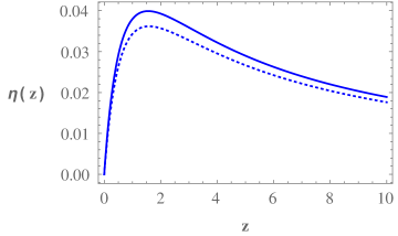
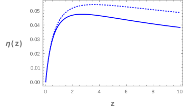
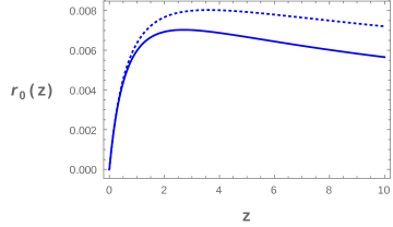
(i) For the most generalized case where , and , let us investigate the solution for the differential equation (60) by applying numerical codes. In this respect, we have employed a numerical code to depict the behavior of the deviation vector in terms of the redshift parameter in the presence of the cosmological constant, see the left panel of the figure 1. (Throughout this paper, we will use the observational data reported in [41].) Although, here we have prepared the figures only for , but our numerical endeavors have shown that the behavior of is affected by the number of the dimensions of spacetime.
(ii) For a particular case where , the analytic solution of equation (60) is given by a complicated function as444To the best of our knowledge, both of the cases (i) and (ii) (concretely, only for associated with the case (ii)) have not been investigated in GR.
| (61) |
where the integration constants and carry the dimension of and is the hypergeometric function.
Moreover, for the special case where , the solution (61) reduces to
| (62) |
The solution (62), by re-scaling the integration constants, has also been obtained in [5].
The relation for the observer area distance is given by
| (63) |
where and stand for the area of the object and the solid angle, respectively. In order to obtain we should employ and assume that the integration constants for are related to each other via . Obviously, without having an exact solution for the deviation vector, it is not possible to obtain an exact expression for .
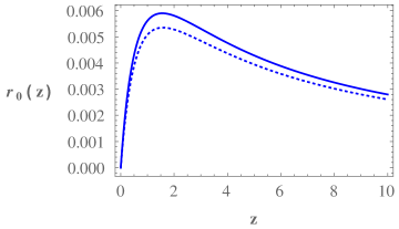
For the case (i), let us focus on numerical approaches to depict the behavior of . In the right panel of figure 1, we have plotted the behavior of for , see the solid curve.
For the case (ii), using (61), we obtain
| (64) | |||||
For the particular case where , we have , therefore equation (64) reduces to
| (65) |
Moreover, concerning the case (ii), for the sake of comparison with the physical CDM model (just as an mathematical exercise), by respecting the equality , we have also plotted the behavior of the observer area distance, see figure 2.
(iii) For another particular case where only vanishes, the behavior of and are shown by the dotted curves in left and right panels of figure 1, respectively.
4 GDE for null vector field in the context of the BD theory
In this section, we would like to apply the GDE (obtained in Section 2) for some well-known exact solutions in the context of the BD theory. Let us first investigate the energy conditions associated with our herein FLRW-BD model. Moreover, we will establish two different dynamical systems associated with the BD cosmological model presented in Section 2. However, for the sake of continuity in the content of this paper, let us present them in A.
4.1 Energy conditions in BD theory of gravity
In Einstein equations, the energy momentum tensor, on the right hand side, determines how the spacetime is curved and hence how the gravity acts. Accordingly, any conditions imposed on the matter-energy distribution immediately affect on the corresponding conditions associated with the geometry in the left hand side. In this respect, the matter-energy distribution establish the causal and geodesic structures of spacetime [42, 43, 44]. Such reasons have encouraged researchers to investigate the energy conditions not only in the standard cosmology but also in models established based on the alternative theories.
4.2 Modified Sen-Seshadri exact solutions in D dimensions
In order to solve the equations (26)-(28) and (32), following [17], let us assume the power law solutions as555It is important to note that, due to a mistake sign in equation (7) of [17], most of our herein equations/relations in the particular case where do not reduce to those obtained in that paper. Therefore, before moving to obtain the GDE associated with herein model, we will present some details regarding the exact solutions as well as the allowed ranges of the parameters of this model.
| (74) | |||
| (75) |
where and are the values of the corresponding quantities at ; and are two parameters. Solutions (74) and (75) lead to take the energy density, pressure and the scalar potential as
| (76) | |||
| (77) | |||
| (78) |
Substituting , and , respectively, from (74), (76) and (77) into (28), we can obtain a relation between and . Another relation between them can be also obtained via employing a combination of the equations (26) and (27) in which should be removed. Therefore, and are obtained. Finally, employing the later relations together with (78) in either (26) or (27), we obtain . In summary, we get
| (79) | |||||
| (80) | |||||
| (81) |
We should note that the quantities and are only two symbols to write the equations (76) and (77) in compact forms (they should have been replaced by other symbols). Concretely, they do not have the same dimension of the energy density, pressure and the potential, but instead, according to the units chosen in this paper (i.e., ), we get .
Before proceeding our discussions concerning the GDE as well as determining the allowed regions for the parameters of our model, let us present an important note about the energy density, pressure as well the EoS parameter associated with the BD scalar field. As mentioned, by imposing the conservation law for the ordinary matter in the BD theory as well as using the Bianchi identity, it is easy to show that and do not satisfy the conservation law, see equation (29). Concretely, it sounds that cannot be considered as a physically meaningful quantity. It has been suggested that a suitable candidate should come from an actual measurable quantity. For the FLRW model, admitting that the is a measurable quantity, it is straightforward to show that where (for more details in four-dimensions, see [40, 39])
| (85) | |||||
| (86) |
can be introduced as a real EoS parameter. More concretely, now and satisfy the conservation law:
| (87) |
We should note that with the new energy density , the Friedmann equation (26) is rewritten as
| (88) |
Consequently, since the tilde quantities are directly related to the observable Hubble parameter and as they satisfy the conservation law, we therefore can consider them for comparing with the predictions of GR [39]. It should be noted that the discrepancy between and is very small [39]. Therefore, for simplicity, let us proceed our investigation with only the non-tilde quantities.
In order to obtain the solutions which could describe the present universe, the range of parameters of the model should be restricted as follows. (i) The range of the deceleration parameter should be restricted such that it would match with the recent observational data [41]. For the power-law solution (74), we have . Therefore, for an accelerating scale factor, must be greater than one. (ii) From relations (79) and (80), the EoS parameter associated with the ordinary matter (as a perfect fluid ), , is:
| (89) |
which should be constrained as . Therefore, we obtain
| (90) |
From equation (90), for and we get .
(iii) The energy densities should take positive values. Therefore, by taking into account the conditions and , from relations (79) and (82), we get the following allowed range for the BD coupling parameter:
| (91) |
On the other hand, should also be restricted as
| (92) |
to get positive values for the energy density associated with the scalar field in the Einstein frame.
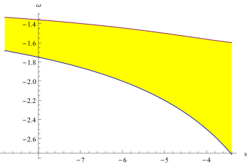
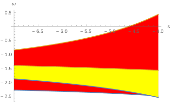
Using (93), the allowed region of can be determined for some particular values of (or ) such that the range of to be in accordance with observational data, see for instance figure 3.
Let us check that whether or not the energy conditions being satisfied for our herein BD cosmology. Substituting the energy density and pressure from relations (76), (77), (82) and (83) into equations (66)-(69), for arbitrary positive values of and , we obtain
| (96) | |||||
| (97) | |||||
| (98) | |||||
| (99) |
It is seen that, assuming an attractive gravity (i.e., ) and an accelerated scale factor, the NEC, WEC and DEC are satisfied for our model. However, in order to satisfy the SEC, inequality (98) yields which cannot be applicable for the present universe.
The GDE equation for this case is obtained by employing relations (74)-(83) in equation (46):
| (100) |
where that can be written as
| (101) |
An analytical exact solution for equation (100) is
| (102) |
where the integration constants and carry the dimension of .
Moreover, by applying (63), we obtain a general formula for the observer area distance associated with the power-law solution for our herein BD model:
| (103) |
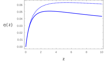
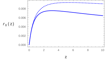
In order to plot and in terms of , we should determine the allowed values of (which, in turn, is a function of , , and ) and the integration constants and . In this regard, we apply the following procedure: (i) we assume and . Therefore (102) yields
| (104) |
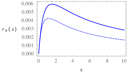
Consequently, with the obtained initial conditions and using the recent observational data [41], we could depict the behavior of the quantities of the model. In figure 4, we have plotted the behavior of the and for some allowed values of the corresponding parameters.
4.3 Standard BD theory
In this section, we restrict our attention to a cosmological application in the context of the standard BD theory for which there is no scalar potential [15]. Moreover, let us assume that the cold matter with negligible pressure is dominated. Therefore, letting , equation (28) yields
| (105) |
As our herein case is indeed a particular case of that presented in the previous subsection, we can retrieve the corresponding solutions from those obtained there. Therefore, using equation (80), we obtain
| (106) |
Moreover, , given by equation (81), should be set equal to zero, we therefore get666Another solution is and . In this case, we obtain and , which corresponds to the matter dominated case in GR.
| (107) |
where we have used (106). Substituting and from relations (106) and (107) into (79), we get
| (108) |
Substituting to equation (76) yields , hence equation (108) can be rewritten as
| (109) |
In summary, the solutions associated with this case are
| (110) | |||||
| (111) | |||||
| (112) |
In the particular case where these relations reduce to those obtained in [15, 18].
Let us proceed our discussions considering the applicability of this model for the late time for which we should have . Therefore, from (110), we obtain
| (113) |
Before moving to focus on the GDE, we would discuss concerning the energy conditions for this case. Again, assuming an attractive gravity and arbitrary values of the cosmic time, it is easy to show that these conditions are satisfied in the following ranges for the BD coupling parameter:
| (114) | |||||
| (115) |
Comparing inequalities (113)-(115), we find that if we demand to get an accelerating scale factor, all the energy conditions are satisfied except the SEC.
Concerning the GDE and its solution as well as the relation associated with the observer area distance, it is straightforward to show that all the relations (100) and (102)-(104) are still valid for this case. However, the relation of corresponding to this case is given by
| (116) |
For , the constraint (113) reduces to . However, as mentioned, to get a positive energy density in the Einstein frame, the BD coupling parameter should be restricted to . Therefore, we should restrict our attention to a very narrow range (which yields a constraint on the deceleration parameter as ), for which we get an accelerating scale factor that is applicable for the present universe.777Although our herein power-law solutions yield accelerating universe, but they have their own problems, which will be discussed in Section 6. For , by taking the allowed values of associated with the accelerating late time universe, the behavior of and has been plotted in figure 5.
5 GDE for null vector field in the context of the MBDT
In what follows, let us present a brief description of the
MBDT in arbitrary dimensions (for more details, see [34]).
In analogy with (2) and (3), we can write the BD field equations in (D+1)-dimensional spacetime as
| (117) |
| (118) |
where we have not assumed any ad hoc scalar potential in -dimensional spacetime (bulk). The Latin indices run from zero to ; all the quantities with superscript and/or Latin indices are associated with the bulk. Moreover, in order to recognize the covariant derivative in the bulk from its corresponding one on the hypersurface, we denote it with an overline, i.e., .
In Ref. [34], by employing an appropriate reduction procedure, it has been shown that the effective field equations on a -dimensional hypersurface can be obtained from (117) and (118). Concretely, it was assumed that the -dimensional spacetime is described by the metric
| (119) |
where is a non-compact coordinate associated with the th dimension; the scalar field depends on all coordinates; is an indicator allows the th dimension to be either time-like or space-like.
By considering that the -dimensional spacetime is foliated by a family of -dimensional hypersurfaces (which, by taking , are denoted by ) being orthogonal to the -dimensional unit vector
| (120) |
along the extra dimension [22, 23], the induced metric is
| (121) |
In summary, it has been eventually shown that the MBDT is described by four sets of effective field equations on the -dimensional spacetime [34]:
-
1.
The equation associated with the scalar field is:
where .
-
2.
By introducing the quantity as
(123) it has been shown that in the MBDT, in contrary to the IMT, this quantity is not conserved, but instead we obtain
(124) -
3.
Another couple of the field equations associated with the -dimensional hypersurface, i.e., the counterpart equations corresponding to (117) and (118), are given by (2) and (3), respectively888It is important to note that equations (3) and (3) are the corrected versions of the corresponding ones presented in [34] (i.e., equations (2.23) and (2.24)). Let us be more precise. In equation (3), the term is multiplied by the coefficient and therefore the wave equation can be obtained from the action (1). We should note that for the particular case where (the main cosmological discussions of [34] have been presented in four dimensions) there are no discrepancies between these equations and those presented in [34]. In order to correct and to complete the results associated with , let us investigate some additional topics in this paper.. However, there is a main difference between the conventional BD theory (presented in Section 2) and the MBDT framework: in contrary to the former, the energy-momentum tensor as well as the scalar potential associated with the latter are not assumed by phenomenological assumptions, but instead they emerge from the geometry of the extra dimension. Let us be more precise. (i) For the MBDT framework, the energy-momentum tensor in equation (2) is given by where and are given by
(125) (126) The three components of in (126) are:
(128) and the term is an induced scalar potential, which is obtained from the following differential equation
In what follows, for later applications, let us mention a few comments.
-
1.
Using the reduction procedure and the metric (119), the field equations (117) and (118) yield four sets of effective equations (2), (3) (for which, the energy-momentum tensor and the potential are obtained from the equations presented in this section rather than phenomenological assumptions), (1) and (124) on the hypersurface.
-
2.
For a special case where and/or , the MBDT framework reduces to the IMT on a -dimensional hypersurface, see [29] and references therein. In order to obtain the equations obtained in [29] from those of the MBDT, in addition to the mentioned conditions, the induced scalar potential, without loss of generality, should be set equal to zero. Therefore, both sides of equation (3) identically vanish. Consequently, equations (1), (2) and (124) reduce to (see also [29])
(130) (131)
In the rest of this section, not only we investigate the GDE in the context of the MBDT
framework, but also we present some modifications to [34] and
analyze new results. First, we should investigate
whether or not the GDE obtained in Section 2 is also valid for the
MBDT framework. For this aim, we should only show that the induced matter on the
hypersurface whether or not obeys the equation of the perfect fluid.
Subsequently, as another application of the GDE, we will obtain exact solutions in the context of the MBDT.
For the cosmological problem in the context of the MBDT, we should restrict our attention to the particular case: (i) we assume there is no ordinary matter in the bulk, i.e., (in order to justify such a specific choice, see, e.g., [27], and references therein); (ii) we impose the cylinder condition [27] (dropping the derivative of all quantities with respect to the -th coordinate ). Consequently, from equations (1), (126), (3) and (3) we obtain
| (133) | |||||
| (134) |
As the components of the induced energy-momentum tensor are essential to compute the GDE, therefore, we let us obtain them. Using (132) and (133), we can easily show that the non-vanishing components of are
| (135) | |||||
| (136) |
where , with no sum.
As it is observed, we have for any and . Namely, the induced energy-momentum tensor associated with the MBDT can be assumed as a perfect fluid with energy density and pressure . Consequently, the energy-momentum tensor associated with our herein noncompact Kaluza-Klein framework can also be expressed by relation (13). Concretely, the formalism of the GDE presented throughout Section 2 (associated with the BD theory with a general scalar potential) are also valid for the MBDT framework. However, it is important to note that for the MBDT case [34], in contrary to the phenomenological procedures used for the BD theory as well as GR, the quantities , and have not been chosen from employing some ad hoc assumptions, but instead we have to use equations (134), (135) and (136).
Assuming , equation (118) yields a constant of motion as
| (137) |
where is an integration constant. On the other hand, from solving equation (134), we get another constant of motion as
| (138) |
where is a constant. Then, from combining equations (137) and (138), we easily obtain a relation between two scalar fields of the model as
| (139) |
where is an integration constant. In the context of the MBDT, we will see that obtaining a relation for as well as using relation (139) assist us to rewrite the GDE equation in terms of the BD scalar field and its derivatives with respect to the cosmic time.
Let us also relate the scalar field to the scale factor. Equations (133), (134) and (139) yield
| (140) | |||||
| (141) |
On the other hand, for the metric (132), we obtain
| (142) |
Substituting quantities (140)–(142) into equation (3), and then using (139), we obtain
| (143) |
which can be written as
| (144) |
where is a constant.999Note that equation (144) can also be easily obtained by substituting from (139) to (137), and therefore . However, for the later applications of equations (140)-(143), we used the above approach. Moreover, this approach may imply the consistency of the field equations of the MBDT.
In order to obtain exact solutions for the field equations, we first obtain the differential equation for the scale factor only: (i) We substitute and from relations (19) and (136) into equation (27). Then, using (139) and (144), we obtain
| (145) |
(ii) By adding equations (26) and (27), and then employing a similar procedure used in (i), we obtain
| (146) |
(iii) It is straightforward to show that combining equations (145) and (146), we can remove :
| (147) |
Equation (147) can be rewritten as
| (148) |
It is easy to show that there is a unique power-law solution for equation (147) as , where and are integration constants and is a function of , and . Consequently, without loss of generality, we can take the solutions of our herein cosmological model as
| (149) |
where and are real parameters and , are nonzero constants. Therefore, is obtained from (139):
| (150) |
We should note that the constants and parameters of the model are not independent. In order to obtain relations among them, substituting the scale factor and the scalar field from (149) to equation (144), we obtain
| (151) |
Moreover, using equation (26), we can obtain a relation between the parameters , and as
| (152) |
Consequently, we can obtain exact expressions of the present quantities of the model. For instance, substituting the scalar field from (149) to equation (141), we obtain the induced scalar potential in terms of as101010There is also an induced scalar potential as a logarithmic function, which, due to the problems related to the energy conditions, will not be studied in this paper.
| (153) |
Moreover, employing (149), (151), (152) and (153), we easily obtain the physical quantities in terms of the cosmic time:
| (154) | |||||
| (155) | |||||
| (156) | |||||
| (157) | |||||
| (158) |
where is given by (152). Furthermore, using relations (152) and (156), we obtain
| (159) |
Before moving to investigate the GDE for this model, let us discuss concerning an important particular case where . Regardless of , when the BD coupling parameter takes vary large values, it is easy to show that (159) reduces to . Moreover, we obtain and . Concretely, in this special case, we retrieve , and the extra dimension decreases with cosmic time for . Consequently, our herein cosmological model for reduces to the spatially flat FLRW model in GR in the absence of the cosmological constant. As this case is not applicable for the late time, we abstain from investigating the GDE for it.
Concerning the solutions for and associated with our herein model, it is easy to show that all the equations (100)-(104) are also valid for this case. In what follows, let us retrieve the allowed ranges of the parameters associated with our herein cosmological model.
-
1.
Letting , we obtain , which implies that can take positive as well as negative values. However, as we would like to have contracting extra dimension [27], we therefore focus on the range .
-
2.
Imposing the positivity condition on and , we obtain
(160) -
3.
Using equations (158) and (160), it is straightforward to show that the allowed region of is:
(161) where . Assuming and the allowed values for (which is obtained from fixing the allowed ranges of and ), we find that always takes negative values. Therefore, letting , taking a specific value for , and substituting the values of from observational data into equation (95), we can easily determine the allowed range in the parameter space .
The above procedure can also be used for obtaining the allowed values of in (101), and we therefore can plot and in terms of the redshift parameter. Since, the behavior of these quantities is similar to those depicted in Section 4, let us abstain from plotting them.
Concerning the energy conditions, we should note that, for our herein MBDT cosmological model, it is straightforward to show that the conditions (96)-(99) are also obtained for this case. Namely, only the SEC is violated when the scale factor is accelerating.
In what follows, let us mention some advantages of our herein MBDT model with respect to the BD model investigated in subsection 4.2. For the similar conditions, it is seen that the allowed ranges for the BD coupling parameter in the MBDT is broader than the corresponding one for the BD framework, see, for instance, figure 6. In the MBDT cosmological model, for every fixed value of (or ), we have another parameter, i.e., (the parameter associated with the extra dimension), which generates the range for . For instance, for a particular case where , and the allowed range of , the allowed range of is specified as , and therefore the allowed range of is shown in figure 6. Assuming that the BD coupling parameter must be greater than (for a four-dimensional spacetime), it is seen that the allowed range of , in the parameter space , associated with the conventional BD model is more narrower than the corresponding one of the MBDT model.
5.1 Matter-dominated universe
For this case, we can use the results obtained above. In order to depict the behavior of and , we should determine the allowed values of , or equivalently, of and . For the matter dominated universe, we should solve equation . Therefore, from using (156) we obtain
| (162) |
where we used the relation (151). We should note that as therefore the extra dimension decreases with cosmic time. In order to compare our herein model with the corresponding case investigated in the context of the standard BD theory (see Subsection 4.3), let us express and in terms of the BD coupling parameter. Substituting and from relation (162) to (152), we can easily obtain such relations. In summary, the solutions associated with the matter-dominated case in the context of the MBDT are:
| (163) | |||||
| (164) | |||||
| (165) | |||||
| (166) | |||||
| (167) |
Moreover, using (151), (152) and (162), the BD coupling parameter can be written as a function of and . On the other hand, for the power-law solution (149), is related to the deceleration parameter as
| (168) |
Consequently, we obtain , and for the matter-dominated case as
| (169) |
Relations (163) and (164) imply that the BD coupling parameter should be restricted as and . On the other hand, as mentioned, the BD coupling parameter should be restricted as in dimensions. Therefore, using this constraints on the relation of in (169), we get
| (170) |
We should note that the inequalities (96)-(99) are also valid for this case. Using relations (163) and (168), these constraints can be written in terms of either or . In this case, we find that only the SEC is violated if we demand to get an accelerating universe.
Let us focus on the four-dimensional universe. Substituting , equation (170) yields
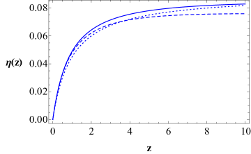
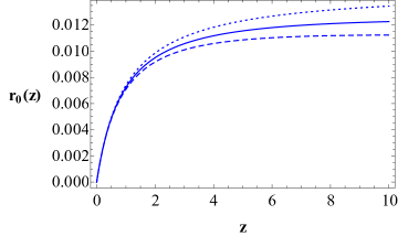
| (171) |
As the deceleration parameter for the present universe is negative, therefore we restrict our attention to the range , which is in accordance with the recent observational reports. Consequently, using relations (101), (157), (158) and (169), we finally obtain . For instance, in Fig. 7, we have plotted the behavior of the deviation vector and the observer area distance in terms of the redshift (see solid curves). As mentioned, our herein model in the limit is not applicable for the present universe [34]. Therefore, for the sake of comparison, we have also depicted the corresponding cases associated with and the standard BD model (discussed in Section 3 and 4.3), see dotted and dashed curves, respectively. It is important to note that our mathematical endeavors show that the behavior of the depicted quantities for all the models are almost similar, see, for instance, figure 7.
In what follows let us emphasize on anther great advantage of our MBDT-FLRW model with respect to the corresponding one obtained in the BD framework. As we have shown in this subsection (for the matter-dominated case), the BD coupling parameter must be restricted as . However, for radiation, i.e., , from (159), we obtain
| (172) |
which implies that for the radiation-dominated case, is not restricted. (For the upper sign, we obtain which is identical to the corresponding case in GR.) This interesting result implies that the reduced cosmology established in the context of the MBDT not only yields an accelerating matter-dominated universe but also it gives a consistent decelerating radiation-dominated universe. Let us compare our herein MBDT model with that investigated in the context of the standard BD theory (see Subsection 4.3): in the latter, the accelerating matter-dominated epoch (where the restriction on is given by (113)) is not consistent with the decelerating radiation-dominated universe for which must be restricted as (in four dimension see [18].) Therefore, in addition to the phenomenological approach employed in [18], another interesting way out of the inconsistency between the matter-dominated and radiation-dominated epoches (faced in the standard BD theory) can be applying the MBDT framework.
6 Conclusions and discussions
In this paper, in analogy with four dimensional spacetime, the field equations associated with the BD theory (including a general scalar potential) were written in arbitrary dimension. Then we restricted our attention to the spatially flat FLRW universe, which is filled with perfect fluid distribution, and obtained the GDE corresponding to our model. Subsequently, we focused on two particular cases, i.e., the fundamental observers and past directed null vector fields, which yield the Raychaudhuri equation and an extended versions of Mattig relation. Moreover, we have obtained a generalized expressions for the Ricci focusing condition, which implies that, in contrary to the corresponding GR case, it depends not only on the components of the ordinary matter fields but also on those associated with the BD scalar field, cf Section 2.
For the particular case where the BD coupling parameter takes large values, the BD scalar field and the potential being constants, we have shown that the results of Section 2 reduce to the generalized version of those obtained for the model. Concerning the latter, we have studied the GDE for three cases, for which, by employing either the exact analytical solutions or the numerical methods, we have depicted the behavior of and , cf Section 3.
Assuming the spatially flat FLRW universe and the BD framework (in the presence of the scalar potential), we have obtained generalized power-law exact solutions in dimensions, which are the corrected as well as modified version of the well-known model investigated in [17]. This model for some different particular cases reduces to those obtained in [15, 47]. We should emphasize that one of our motivations in choosing the cosmological models with a self-interaction potential was to describe the epochs of the universe with small values of the redshift parameter, which, in turn, are suitable for applying our herein GDE for null vector field.
Moreover, we have investigated the energy conditions for our herein BD cosmology and then applied them to the our exact solutions. We have shown that, if we demand to apply these solutions for the late time universe, only the SEC is violated.
It has been believed that the cosmological models studied in Section 4 face with a few problems: (i) The allowed range of the BD coupling parameter that yields an accelerating scale factor associated with the matter-dominated epoch cannot generate a consistent model with the radiation-dominated duration. An appropriate method to overcome to this problem can be generalizing that model such that the constant is replaced by a varying one, i.e., [18]. (ii) Almost in all of the BD cosmological models, the acceleration as well as coincidence problems are solved provided that the takes low negative values, which is inconsistent with its lower limit imposed by solar system experiments [48]. (iii) The components of the energy-momentum tensor associated with the BD scalar field, in contrary to those of the ordinary matter, do not satisfy the conservation law. In this respect, we defined other corresponding tilde quantities, which not only are related to the measurable quantities of the model but also satisfy the conservation law. However, due to very tiny discrepancy between the and , we eventually proceeded our discussions with the un-tilde quantities.
For all the cosmological models presented in Section 4, we investigated the corresponding GDE for null vector field and depicted the behavior of the quantities and .
In order to have comprehensive discussions of the GDE in the context of the BD models, we have also considered the modified frameworks related to the modern Kaluza-Klein theories [27]. More concretely, the GDE has also been investigated in the MBDT whose energy-momentum tensor and potential are described in terms of geometrical quantities. In this regard, we have shown that all the results obtained in Section 2 can also be applied for the MBDT framework. In order to analyze the GDE for null vector field for this case, we obtained the exact solutions where the components of the matter as well as the scalar potential emerge from the geometry of the extra dimension. We have mentioned the advantages of the MBDT-FLRW cosmology with respect to the corresponding one studied in the conventional BD theory. In this respect, we have also shown that the MBDT cosmological model, in contrast to the corresponding model obtained in the conventional BD framework, yields consistent radiation-dominated and matter-dominated epochs.
Then, we have obtained the analytical exact solutions for and , whose behavior have been depicted for this case and they have also been compared with those associated with GR and BD models. We have shown that the quantities and for all the mentioned models have similar behaviors for small values of , as expected.
We have shown that for both the BD theory and the MBDT cosmological models in arbitrary dimensions (studied in 4.2 and 5), the Ricci forcing condition (35) yields . Concretely, for an expanding universe in both of these models all families of null geodesics experience focusing. Moreover, assuming a vacuum fluid (cosmological constant) in the context of the BD theory (), the focusing condition leads to a constraint on the parameters of the model as .
In order to provide a complete description of the frameworks presented in Sections 2 and 5, we have employed two different procedures to establish the most general dynamical systems. In the first approach, assuming a general power-law scalar potential, we have obtained three coupled second order equations. In some particular case, this dynamical setting reduces to those investigated in [49, 50]. However, in the second approach, we did not impose any condition on the form of the scalar potential. Both of these frameworks can be appropriate settings to analyze the BD-FLRW cosmological models. Moreover, it worth noting that studying the evolution of the density perturbation is important not only to check the stability of the model but also to compare the results of our herein cosmological models with their corresponding observational data. However, we should emphasize that investigating these structures have not been as the main objectives of the present paper. Therefore, we abstained from presenting a full analysis of these interesting settings, but instead, in order to apply the results of Section 2, we merely paid our attention to a few particular classes of the exact solutions, which can be considered as special subclasses generated by our herein dynamical systems. Consequently, for the sake of continuity of the content of this paper, we presented the general formalism of the dynamical systems in A.
7 Acknowledgements
We are very grateful to Prof. Anupam Mazumdar and K. Atazadeh for their constructive comments. We would like to thank the anonymous reviewers for their careful reading of the paper and the valuable comments. SMMR acknowledges the FCT grants UID-B-MAT/00212/2020 and UID-P-MAT/00212/2020 at CMA-UBI. Moreover, SMMR sincerely thanks Fatimah Shojai for giving the opportunity for visiting the University of Tehran. FS is grateful to the University of Tehran for supporting this work under a grant provided by the university research council.
Appendix A Dynamical system approach for a generalized BD theory
The dynamical system theory has been employed as a powerful mathematical tool for investigating the cosmological models within the context of GR as well as alternative theories, see, for instance [51, 52, 53, 54, 55, 56, 57, 58, 59, 60, 61, 62] and references therein. It has been believed that large classes of exact solutions obtained in the context of BD theory could be recovered from a corresponding suitable dynamical system, see for instance [52]. Obviously, any class of the exact solutions corresponding to the set of equations (26)-(28) are associated with a special choice of the initial conditions. Therefore, presenting a qualitative analysis of the dynamical system corresponding to a cosmological model sounds to be a reasonable approach. Subsequently, translating the results to the physically meaningful - plane, if possible, provides a complete description of the model. In this respect, let us establish two dynamical settings for our herein cosmological mode. However, investigating the dynamical scenario has not been in the scope of the present investigation, but instead, we have only restricted our attention to some well-known examples to observe whether or not our herein GDE does work well. In this regard, we present our dynamical systems in this section.
In the first approach, using new variables, we transform the fourth-order system (26)-(28) and (32) into three coupled second-order equations. Let use the conformal time as and define the following variables
| (173) | |||||
| (174) |
where a prime denotes differentiation with respect to .
Moreover, assuming a power-law scalar potential given by and a barotropic matter described by (where is a constant and , are two real parameters), it is straightforward to show that equations (32) and (26), respectively, transform to
| (175) | |||||
| (176) |
Finally, letting , a generalized three-dimensional dynamical system is retrieved for our herein model:
| (177) | |||||
| (178) | |||||
| (179) |
For the spatially flat FLRW model, the set (177)-(179) can be considered as the most extended case scenario obtained in the context of BD theory. Let us mention a few special cases: (i) For and , this model reduces to what investigated in [63]. (ii) Assuming , the Z-equation disappears and we get a two-dimensional dynamical system, which for , we recover the model studied in [49].
Let us also provide the second dynamical system associated with our herein BD cosmological model. Defining new variables as
| (180) | |||||
| (181) | |||||
| (182) |
it is straightforward to show that the Friedmann equation and the acceleration equation can be written as
| (183) | |||||
| (184) | |||||
| (186) |
Introducing , we easily show that the following 3-dimensional dynamical system can describe our herein D-dimensional BD model:
| (187) | |||||
| (189) | |||||
| (190) | |||||
| (191) |
where
| (192) |
In the particular case where , the above dynamical system reduces to that investigated in [64] in which the dynamics for the specific case of the quadratic scalar potential has been analyzed.
Moreover, if we assume that, in addition to the presence of the scalar potential, the BD coupling parameter depends also on the BD scalar field, the most generalized dynamical system associated with the scalar-tensor theories is obtained. A particular case of this model where and has been established in [58].
Again, we emphasize that we abstained form presenting complete analysis of the above dynamical systems in this paper. Instead, we focused on a few specific exact solutions, which might be generated from the above dynamical system formalisms.
References
- [1] J. L. Synge, Ann. Math. 35, 705 (1934).
- [2] F. A. E. Pirani, Acta Phys. Polon. 15, 389 (1956).
- [3] F. A. E. Pirani, Phys. Rev. 105, 1089 (1957).
- [4] P. Szekeres, J. Maths. Phys. 6, 1387 (1965).
- [5] George F.R. Ellis and Henk van Elst, “Deviation of geodesics in FLRW spacetime geometries”, arXiv: gr-qc/9709060.
- [6] F. Shojai and A. Shojai, Phys. Rev. D 78, 104011 (2008).
- [7] A. Guarnizo, L. Castañeda ·and Juan M. Tejeiro, Gen. Relativ. Gravit. 43, 2713 (2011).
- [8] Ines G. Salako, M. J. S. Houndjo and Abdul Jawad, Int. J. of Mod. Phys. D 25, 1650076 (2016).
- [9] S. M. M. Rasouli, A. F. Bahrehbakhsh, S. Jalalzadeh and M. Farhoudi, EPL 87 40006 (2009).
- [10] F. Darabi, M. Mousavi and K. Atazadeh, Phys. Rev. D 91 084023 (2015).
- [11] D. Sáez and V. J. Ballester,Phys. Lett.113A, 9, 1986.
- [12] S. M. M. Rasouli, R. Pacheco, M. Sakellariadou and P. V. Moniz Physics of the Dark Universe 27, 100446 (2020).
- [13] S. M. M. Rasouli, M. Sakellariadou and P. V. Moniz, “Geodesic Deviation in Sáez-Ballester theory in arbitrary dimensions”, in progress.
- [14] P. Mukherjee and S. Chakrabarti, Eur. Phys. J. C 79, 681 (2019).
- [15] C. Brans and R.H. Dicke, Phys. Rev. 124, 925 (1961).
- [16] S. Sen and A.A. Sen, Phys. Rev. D 63, 124006 (2001).
- [17] S. Sen and T. R. Seshadri, Int. J. Mod. Phys. D 12, 445 (2003).
- [18] N. Banerjee and D. Pavon, Phys. Rev. D 63, 043504 (2001).
- [19] L. E. Mendesa and A. Mazumdar, Phys. Lett. B 501, 249 (2001).
- [20] L. Qiang, Y. Ma, M. Han and D. Yu, Phys. Rev. D 71, 061501 (2005).
- [21] Li-e Qiang, Yan Gonga, Yongge Ma and Xuelei Chena, Phys. Lett. B 681, 210 (2009).
- [22] J. Ponce de Leon, Class. Quant. Grav. 27, 095002 (2010).
- [23] J. Ponce de Leon, J. Cosmol. Astropart. Phys. 03, 030 (2010).
- [24] S.M. M. Rasouli, M. Farhoudi and H.R. Sepangi, Class. Quant. Grav. 28, 155004 (2011).
- [25] S. M. M. Rasouli and P. V. Moniz Class. Quantum Grav. 35, 025004 (2018).
- [26] P.S. Wesson and J. Ponce de Leon, J. Math. Phys. 33, 3883 (1992).
- [27] J.M. Overduin and P.S. Wesson, Phys. Rep. 283, 303 (1997).
- [28] P.S. Wesson, Space–Time–Matter: Modern Kaluza–Klein Theory (World Scientific, Singapore, 1999).
- [29] S. Rippl, C. Romero and R. Tavakol, Class. Quant. Grav. 12, 2411 (1995).
- [30] A. A. Garcí, A. García-Quiroz, M. Cataldo and Sergio del Campo, Phys. Rev. D 69, 041302 (2004).
- [31] Alberto A. Garcia and Steve Carlip, Phys. Lett. B 645, 101 (2007).
- [32] P. S. Letelier and J. P. M. Pitelli, Phys. Rev. D 82, 104046 (2010).
- [33] Arzu Coruhlu Tanismana, Mustafa Saltib, Hilmi Yanarc and Oktay Aydogdud, Eur. Phys. J. Plus 134, 325 (2019).
- [34] S.M. M. Rasouli, M. Farhoudi and P. V. Moniz, Classical Quantum Gravity 31, 115002 (2014).
- [35] N. Doroud, S.M. M. Rasouli and S. Jalalzadeh, Gen. Rel. Grav. 41, 2637 (2009).
- [36] S.M. M. Rasouli and S. Jalalzadeh, Ann. Phys. (Berlin) 19, 276 (2010).
- [37] S. M. M. Rasouli, J. Marto and P. V. Moniz Physics of the Dark Universe 24, 100269 (2019).
- [38] Ray D́ Inverno, Introducing Einstein’s Relativity, (Oxsford University Press, Cambridge, 1992).
- [39] Diego F. Torres, Phys. Rev. D 66, 043522 (2002).
- [40] V. Faraoni, Cosmology in Scalar Tensor Gravity (Kluiwer Academic Publishers, Netherlands, 2004).
- [41] Planck Collaboration, N. Aghanim, et al., Planck 2018 results VI: “Cosmological parameters” arXiv:1807.06209.
- [42] S.W. Hawking, G.F.R. Ellis, The Large Scale Structure of Space–Time, (Cambridge University Press, Cambridge, 1973).
- [43] R.M. Wald, General Relativity, (The University of Chicago Press, Chicago, 1984).
- [44] Salvatore Capozziello, Francisco, S.N. Lobo and José P. Mimoso, Phys. Lett. B 730, 280 (2014).
- [45] M. Sharif and Saira Waheed, Advances High Energy Phys. 2013, 253985 (2013).
- [46] Hideki Maeda, Cristián Martínez, “Energy conditions in arbitrary dimensions”, Progress of Theoretical and Experimental Physics 2020, 4 (2020), arXiv:1810.02487.
- [47] O. Bertolami and P. J. Martins, Phys. Rev. D 61, 064007 (2000).
- [48] B. Bertotti, L. Iess, and P. Tortora, Nature 425, 374 (2003).
- [49] S. J. Kolitch, and D. M. Eardley, Ann. Phys. (N.Y.) 241, 128 (1995).
- [50] Damien J. Holden and David Wands, Class. Quantum Grav. 15, 3271 (1998).
- [51] J. Wainwright and G. F. R. Ellis, eds., Dynamical Systems in Cosmology, (Cambridge University Press, Cambridge, 1997).
- [52] C. Romero and H. P. Oliveira Astrophysics and Space Science 159, 1-9 (1989).
- [53] Valerio Faraoni, Annals of Physics 317, 366 (2005).
- [54] Laur Järv and Piret Kuusk, Phys. Rev. D 78, 083530 (2008).
- [55] Piret Kuusk, Laur Järv and Erik Randla, “Scalar-Tensor and Multiscalar-Tensor Gravity and Cosmological Models”, Springer Proceedings in Mathematics and Statistics 85, DOI: , Springer-Verlag Berlin Heidelberg (2014).
- [56] M. Sharif and Rubab Manzoor Eur. Phys. J. C 76, 330 (2016).
- [57] G. Papagiannopoulos, John D. Barrow, S. Basilakos, A. Giacomini, and A. Paliathanasis, Phys. Rev. D 95, 024021 (2017).
- [58] N. Roy and N. Banerjee, Phys. Rev. D 95, 064048 (2017).
- [59] S. D. Odintsov and V. K. Oikonomou, Phys. Rev. D 96, 104049 (2017).
- [60] Jianbo Lu, Xin Zhao, Shining Yang, Jiachun Li and Molin Liu, Int. J. of Mod. Phys. D 28, 1950132 (2019).
- [61] Alex Giacomini, Genly Leon, Andronikos Paliathanasis and Supriya Pan, Eur. Phys. J. C 80, 184 (2020).
- [62] Jonghyun Sim, Jiwon Park and Tae Hoon Lee, Mod. Phys. Lett. A 35, 2050094 (2020).
- [63] C. Santos and R. Gregory Annals of Phys. 258, 111 (1997).
- [64] O. Hrycyna and M. Szydlowski, JCAP 12 016 (2013).