The mean free path of ionizing photons at 5 < z < 6: evidence for rapid evolution near reionization

Abstract

The mean free path of ionizing photons, $\lambda_{\rm mfp}$, is a key factor in the photoionization of the intergalactic medium (IGM). At $z\gtrsim 5$, however, $\lambda_{\rm mfp}$ may be short enough that measurements towards QSOs are biased by the QSO proximity effect. We present new direct measurements of $\lambda_{\rm mfp}$ that address this bias and extend up to $z\sim 6$ for the first time. Our measurements at $z\sim 5$ are based on data from the Giant Gemini GMOS survey and new Keck LRIS observations of low-luminosity QSOs. At $z\sim 6$ we use QSO spectra from Keck ESI and VLT X-Shooter. We measure $\lambda_{\rm mfp}=9.09^{+1.62}_{-1.28}$ proper Mpc and $0.75^{+0.65}_{-0.45}$ proper Mpc (68% confidence) at $z=5.1$ and 6.0, respectively. The results at $z=5.1$ are consistent with existing measurements, suggesting that bias from the proximity effect is minor at this redshift. At $z=6.0$, however, we find that neglecting the proximity effect biases the result high by a factor of two or more. Our measurement at $z=6.0$ falls well below extrapolations from lower redshifts, indicating rapid evolution in $\lambda_{\rm mfp}$ over $5<z<6$. This evolution disfavors models in which reionization ended early enough that the IGM had time to fully relax hydrodynamically by $z=6$, but is qualitatively consistent with models wherein reionization completed at $z=6$ or even significantly later. Our mean free path results are most consistent with late reionization models wherein the IGM is still 20% neutral at $z=6$, although our measurement at $z=6.0$ is even lower than these models prefer.

1 Introduction

The metagalactic UV background is a fundamental link between the intergalactic medium (IGM) and the sources of ionizing radiation (stars and active galactic nuclei). Much of our knowledge of the IGM comes from observations of the Ly$\alpha$ forest, whose opacity depends directly on the hydrogen ionization rate, $\Gamma$. For a given ionizing emissivity, $\epsilon$, the ionization rate scales roughly as $\Gamma\propto\epsilon\lambda_{\rm mfp}$ (e.g., Haardt & Madau, 2012), where $\lambda_{\rm mfp}$ is the mean free path of ionizing photons. Accurate measurements of $\lambda_{\rm mfp}$ are therefore essential for translating the measured properties of the IGM into constraints on the ionizing sources.

The redshift evolution of $\lambda_{\rm mfp}$ may also reflect the timing of reionization (e.g., Rahmati & Schaye, 2018). A number of observations now suggest that reionization had a midpoint around $z\sim$7–8 and ended near $z\sim 6$, or even later. These include (i) the electron optical depth to CMB photons (Planck Collaboration et al., 2020), (ii) the decline in Ly$\alpha$ emission from galaxies at $z>6$ (e.g., Jung et al., 2020; Morales et al., 2021, and references therein), (iii) large-scale opacity fluctuations in the Ly$\alpha$ forest at $z<6$ (Fan et al., 2006; Becker et al., 2015; Bosman et al., 2018; Eilers et al., 2018; Yang et al., 2020), (iv) the association of large Ly$\alpha$ troughs at $z\sim 5.7$ with galaxy underdensities (Becker et al., 2018; Kashino et al., 2020), (v) Ly$\alpha$ damping wings seen in the spectra of $z\sim 7$ QSOs (Mortlock et al., 2011; Greig et al., 2017, 2019; Davies et al., 2018; Bañados et al., 2018; Wang et al., 2020), (vi) the thermal history of the IGM at $z>5$ (Boera et al., 2019; Walther et al., 2019; Gaikwad et al., 2020), and (vii) the evolution in the number density of neutral metal absorbers near $z\sim 6$ (Becker et al., 2011, 2019; Cooper et al., 2019; Doughty & Finlator, 2019). If reionization did end near or below $z=6$, then the mean free path at $z<6$ should increase rapidly with time as large H ii bubbles merge and the last remaining neutral islands are ionized (e.g., Wyithe et al., 2008). Indeed, recent models of late reionization exhibit a rapid evolution in $\lambda_{\rm mfp}$ over $5<z<6$ (e.g., Kulkarni et al., 2019; Keating et al., 2020a, b; Cain et al., 2021). Additionally, absorbers in recently reionized gas are photoevaporated or pressure smoothed over a time scale $\Delta t\sim 100$ Myr, contributing further to the rapid evolution in LyC opacity. In constrast, a significantly earlier reionization would give the IGM more time to relax hydrodynamically, producing a more gradual evolution in $\lambda_{\rm mfp}$ at $z<6$ (Park et al., 2016; D’Aloisio et al., 2020; Cain et al., 2021).

Multiple techniques have been used to measure the mean free path. One approach is to calculate the ionizing opacity from the incidence rate of individual H i absorbers (e.g., Miralda-Escude & Ostriker, 1990; Meiksin & Madau, 1993; Haardt & Madau, 1996; Faucher-Giguère et al., 2008; Songaila & Cowie, 2010; Rudie et al., 2013; Prochaska et al., 2014). Alternatively, one may directly estimate the opacity from the shape of the transmitted flux profile blueward of the Lyman limit in the mean spectra of QSOs (Prochaska et al., 2009). The latter approach has arguably produced the most precise estimates of the mean free path at high redshifts, with results now spanning $2\lesssim z\lesssim 5$ (Prochaska et al., 2009; Fumagalli et al., 2013; O’Meara et al., 2013; Worseck et al., 2014; Lusso et al., 2018). One can also infer the mean free path from the average of free paths along individual QSO lines of sight (Romano et al., 2019).

One challenge at $z>5$ is that the mean free path may be comparable to or shorter than the typical size of a QSO proximity zone. In that case, the ionizing flux from a QSO will tend to decrease the opacity in its vicinity, leading to mean free path measurements based on QSO spectra that are biased high (e.g., Worseck et al., 2014; D’Aloisio et al., 2018). One possible solution is to use fainter QSOs, for which the impact of the proximity zone will be decreased (see discussion in Worseck et al., 2014). This is observationally challenging, however, particularly given the low levels of transmission expected at $z\gtrsim 5.5$. At $z\sim 6$ it is currently impractical to obtain enough high-quality spectra of QSOs that are sufficiently faint to meaningfully avoid the proximity effect.

In this work we perform new measurements of the mean free path at $z>5$, including the first direct measurement at $z\sim 6$, that address the proximity effect in two ways. First, we modify the direct measurement approach of Prochaska et al. (2009) to include a scaling of the opacity with the local ionization rate. This allows us to account for the decrease in opacity in the vicinity of a QSO. Second, we measure $\lambda_{\rm mfp}$ at $z\simeq 5$ from two groups of QSOs spanning a factor of five in mean luminosity. This provides additional leverage in separating the background opacity from the impact of the QSOs.

The rest of the paper is organized as follows. We describe the individual QSO spectra and the composites in Section 2. In Section 3 we outline our model formalism, perform tests with mock spectra, and derive measurements of $\lambda_{\rm mfp}$. We then discuss the implications of our results for reionization in Section 4 before summarizing the results in Section 5. Our observational results assume a $\Lambda$CDM cosmology with $(\Omega_{\rm m},\Omega_{\Lambda},H_{0})=(0.3,0.7,70~{}{\rm km\;s^{-1}\;Mpc^{-1}})$. Distances are quoted in proper Mpc (pMpc) except where noted.

2 Data

2.1 Samples

This work uses spectra from three QSO samples. First, we use a subset of the spectra from the Giant Gemini GMOS (GGG) survey presented by Worseck et al. (2014). Specifically, we use 40 QSOs spanning $5.00<z<5.42$, which have a mean redshift of $\langle z\rangle=5.16$ and an absolute magnitude corresponding to the mean luminosity at rest-frame 1450 Å of $M_{1450}=-26.8$. Second, we include a sample of lower-luminosity QSOs at $z\sim 5$ observed with the Keck LRIS spectrograph. The LRIS sample includes 23 QSOs spanning $4.93<z<5.24$ with $\langle z\rangle=5.09$ and an absolute magnitude corresponding to the mean luminosity of $M_{1450}=-25.1$. This is a factor of five fainter than the GGG sample. Finally, we use a sample of 13 QSOs at $z\sim 6$ observed with the Keck ESI and VLT X-Shooter spectrographs. This sample spans $5.82<z<6.08$ with $\langle z\rangle=5.97$ and an absolute magnitude corresponding to the mean luminosity of $M_{1450}=-27.0$. The samples are summarized in Table 1, and the QSOs included in each sample are listed in Table 2. We plot the rest-frame 1450 Å absolute magnitudes as a function of redshift for all of our QSOs in Fig. 1.

Table 1: QSO samples analyzed in this work

Sample	$n_{\rm qso}$	$\langle z_{\rm qso}\rangle$	$M_{1450}$
GGG	40	5.16	$-26.6$
LRIS	23	5.09	$-25.1$
ESI + X-Shooter	13	5.97	$-27.0$

For we each sample we list the number of QSOs, the mean redshift, and the absolute magnitude at rest-frame 1450 Å corresponding to the mean luminosity.

Table 2: QSOs analyzed in this work

QSO	Instrument	$z_{\rm qso}^{a}$	$M_{1450}^{b}$
SDSS J0231$-$0728	GMOS	5.420	$-$26.6
SDSS J0338$+$0021	GMOS	5.040	$-$26.7
SDSS J0824$+$1302	GMOS	5.207	$-$26.2
SDSS J0846$+$0800	GMOS	5.028	$-$26.9
SDSS J0854$+$2056	GMOS	5.179	$-$27.0
SDSS J0902$+$0851	GMOS	5.226	$-$25.9
SDSS J0913$+$5919	GMOS	5.122	$-$25.3
SDSS J0915$+$4924	GMOS	5.199	$-$26.9
SDSS J0922$+$2653	GMOS	5.042	$-$26.0
SDSS J0957$+$0610	GMOS	5.167	$-$27.6
SDSS J1026$+$2542	GMOS	5.254	$-$26.5
SDSS J1050$+$5804	GMOS	5.151	$-$26.5
SDSS J1053$+$5804	GMOS	5.250	$-$27.0
SDSS J1054$+$1633	GMOS	5.154	$-$26.4
SDSS J1101$+$0531	GMOS	5.045	$-$27.7
SDSS J1132$+$1209	GMOS	5.180	$-$27.2
SDSS J1148$+$3020	GMOS	5.128	$-$26.3
SDSS J1154$+$1341	GMOS	5.060	$-$25.6
SDSS J1202$+$3235	GMOS	5.298	$-$28.1
SDSS J1204$-$0021	GMOS	5.094	$-$27.4
SDSS J1209$+$1831	GMOS	5.127	$-$26.8
SDSS J1221$+$4445	GMOS	5.203	$-$25.8
SDSS J1222$+$1958	GMOS	5.120	$-$25.5
SDSS J1233$+$0622	GMOS	5.300	$-$26.2
SDSS J1242$+$5213	GMOS	5.036	$-$25.7
SDSS J1334$+$1220	GMOS	5.130	$-$26.8
SDSS J1337$+$4155	GMOS	5.018	$-$26.6
SDSS J1340$+$2813	GMOS	5.349	$-$26.6
SDSS J1340$+$3926	GMOS	5.048	$-$26.8
SDSS J1341$+$3510	GMOS	5.252	$-$26.6
SDSS J1341$+$4611	GMOS	5.003	$-$25.4
SDSS J1423$+$1303	GMOS	5.048	$-$27.1
SDSS J1436$+$2132	GMOS	5.227	$-$26.8
SDSS J1437$+$2323	GMOS	5.320	$-$26.8
SDSS J1534$+$1327	GMOS	5.043	$-$25.0
SDSS J1614$+$2059	GMOS	5.081	$-$26.6
SDSS J1614$+$4640	GMOS	5.313	$-$25.8
SDSS J1626$+$2751	GMOS	5.265	$-$27.8
SDSS J1659$+$2709	GMOS	5.316	$-$27.7
SDSS J2228$-$0757	GMOS	5.150	$-$26.1
J0015$-$0049	LRIS	4.931	$-$25.2
J0023$-$0018	LRIS	5.037	$-$25.1
J0108$-$0100	LRIS	5.118	$-$24.6
J0115$+$0015	LRIS	5.144	$-$25.1
J0129$-$0028	LRIS	5.015	$-$25.1
J0208$-$0112	LRIS	5.231	$-$25.3
J0221$-$0342	LRIS	5.024	$-$24.9
J0236$-$0108	LRIS	4.974	$-$25.0
J0256$+$0002	LRIS	4.960	$-$24.6
J0321$+$0029	LRIS	5.041	$-$24.9
J0338$+$0018	LRIS	4.988	$-$25.1
J0349$+$0034	LRIS	5.209	$-$25.3
J1408$+$5300	LRIS	5.072	$-$25.5
J1414$+$5732	LRIS	5.188	$-$24.8
J2111$+$0053	LRIS	5.034	$-$25.3
J2202$+$0131	LRIS	5.229	$-$24.6
J2211$+$0011	LRIS	5.237	$-$24.8
J2226$-$0109	LRIS	4.994	$-$24.6
J2233$-$0107	LRIS	5.104	$-$25.0
J2238$-$0027	LRIS	5.172	$-$25.1
J2239$+$0030	LRIS	5.092	$-$25.2
J2312$+$0100	LRIS	5.082	$-$25.6
J2334$-$0010	LRIS	5.137	$-$24.6

Table 2: – continued

QSO	Instrument	$z_{\rm qso}^{a}$	$M_{1450}$
SDSS J0002$+$2550	ESI	5.824	$-$27.3
SDSS J0005$-$0006	ESI	5.851	$-$25.7
SDSS J0818$+$1722	X-Shooter	6.001	$-$27.5
SDSS J0836$+$0054	X-Shooter	5.805	$-$27.8
SDSS J0840$+$5624	ESI	5.853	$-$27.2
SDSS J0842$+$1218	X-Shooter	6.0754d	$-$26.9
SDSS J1137$+$3549	ESI	6.030	$-$27.4
ULAS J1207$+$0630	X-Shooter	6.0366c	$-$26.6
SDSS J1306$+$0356	X-Shooter	6.0330d	$-$26.8
SDSS J1411$+$1217	ESI	5.920	$-$26.7
SDSS J1602$+$4228	ESI	6.084	$-$26.9
SDSS J2054$-$0005	ESI	6.0389d	$-$26.2
PSO J340$-$18	X-Shooter	6.0007e	$-$26.4

^aRedshifts for GMOS QSOs are adopted from Worseck et al. (2014). Other redshifts quoted to three decimal places are based on the apparent start of the Ly$\alpha$ forest. See text for details.

^b$M_{1450}$ values for GMOS QSOs were calculated from the flux-calibrated spectra published by Worseck et al. (2014). For LRIS QSOs they are adopted from McGreer et al. (2013, 2018). For ESI and X-Shooter QSOs the $M_{1450}$ values are from Bañados et al. (2016) and references therein.

^c[C ii] 158 $\mu$m redshift from Decarli et al. (2018)

^d[C ii] 158 $\mu$m redshift from Venemans et al. (2020)

^eLy$\alpha$ halo redshift from Farina et al. (2019)

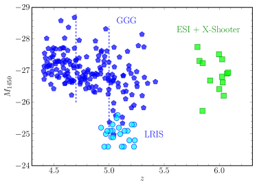
Figure 1: Absolute magnitude at rest-frame 1450 Å versus redshift for the QSOs in this work. The full GGG sample from Worseck et al. (2014) is shown for reference (dark blue pentagons) with vertical dashed lines marking their redshift bins. In this work we analyze the GGG QSOs at $z>5$, along with the samples observed with LRIS (light blue circles) and ESI + X-Shooter (green squares). Details of the individual QSOs are given in Table 2.

2.2 GGG spectra

Our subset of the GGG data includes all objects at $z>5$ observed in that survey apart from one flagged as a broad absorption line (BAL) QSO and one whose flux was affected by very poor sky subtraction. The 40 QSOs selected are listed in Table 2. Details of the observation and data reduction are given in Worseck et al. (2014). Here we note that the Lyman continuum portion of the spectra were observed with the GMOS B600 grating through a 1” slit, which gives a FWHM resolution of roughly 320 km s^-1. We also note that the spectra contain noticeable variations in the sky-level zero point, as discussed by Worseck et al. (2014). We account for these variations when fitting models to the mean flux profile (see Section 3).

2.3 LRIS observations

We observed 27 faint ($M_{\rm 1450}\sim-25$) $z\sim 5$ QSOs in March and September 2019 using the Keck Low Resolution Imaging Spectrometer (LRIS; Oke et al., 1995). The targets were drawn from the surveys for faint QSOs conducted by McGreer et al. (2013, 2018) in the SDSS Stripe 82 and the CFHT Legacy Survey fields. We used a $1.0\arcsec$ slit with the D680 dichroic. On the blue side we used the 300/5000 grism, which provided the maximum sensitivity near the Lyman limit for the QSOs in our sample (observed wavelengths near 5400–5700 Å). The resolution from this grism is relatively low (${\rm FWHM}\simeq 490$ km s^-1, measured from skylines) but sufficient for the mean free path measurement described in Section 3. On the red side we used the 831/8200 grating (${\rm FWHM}\simeq 110$ km s^-1) centered at 7989 Å, which allowed us to identify individual absorption lines near the start of the Ly$\alpha$ forest.

The spectra were reduced using a custom reduction package similar to the one described in Becker et al. (2012) and Lopez et al. (2016). Individual frames were sky-subtracted using an optimal algorithm based on Kelson (2003). Preliminary one-dimensional spectra were then optimally extracted following Horne (1986) . For each exposure, a telluric absorption model was fit to the red side and then propagated back to the two-dimensional sky-subtracted frames for both the blue and the red side. A final one-dimensional spectrum for each side was then extracted simultaneously from all exposures of a given object. One complication of our chosen setup is that the D680 dichroic combined with the 300/5000 grism allows contamination from second-order light. This is nominally not a problem for our QSOs, which have essentially no flux blueward of $\sim$5000 Å; however, it does impact the spectra of blue standard stars, which in turn can impact the flux calibration reward of $\sim$6000 Å. We addressed this problem by using the type dG-K standard star G158-100, whose flux peaks near 5000 Å and declines rapidly towards the blue. Flux calibration derived from this standard produced a good match between the blue- and red-side spectra of our QSOs. The blue (red) side was extracted in wavelength bins of 120 (60) km s^-1.

Out of this sample, 23 QSOs were selected to create the composite described in Section 2.6. These objects are listed in Table 2 and their spectra are plotted in Appendix A. The remaining four QSOs were rejected either due to the presence of BAL features (J2245$+$0024, J0210$+$0003, J0218$-$002) or due to difficulty in measuring the redshift (J0215$-$0529).

2.4 ESI and X-Shooter spectra

Our $z\sim 6$ sample is drawn from the Keck ESI and VLT X-Shooter spectra used by Becker et al. (2019). A lower redshift bound of $z>5.8$ was chosen so that the entire spectrum blueward of the Ly$\alpha$ emission line down to a rest-frame wavelength of 820 Å falls entirely in the VIS arm of X-Shooter. An upper bound of $z<6.1$ was chosen so that the Lyman series opacity of the IGM still allows some possibility of measuring flux blueward of the Lyman limit. Due to the high sensitivity required to detect any continuum transmission at these redshifts, we also required a minimum signal-to-noise ratio in the continuum near rest-frame 1285 Å of $S/N\geq 20$ per 30 km s^-1 interval. After rejecting BALs and objects with strong associated metal absorption and/or associated Ly$\alpha$ damping wing absorption (typically with associated narrow metal lines), we selected 13 QSOs. These are listed in Table 2. The mean redshift in this sample is $\langle z_{\rm qso}\rangle=5.97$. As described in Becker et al. (2019), the ESI spectra have a typical resolution of ${\rm FWHM}\simeq 45$ km s^-1 and were extracted in bins of 15 km s^-1, while the X-Shooter spectra have a typical resolution of ${\rm FWHM}\simeq 25$ km s^-1 in the VIS arm and were extracted in bins of 10 km s^-1. Individual spectra are plotted in Appendix A. The rarity of obvious transmitted flux blueward of the Lyman limit highlights the challenge of directly measuring $\lambda_{\rm mfp}$ at these redshifts.

2.5 QSO redshifts

Following Worseck et al. (2014), we measured QSO redshifts from the apparent start of Ly$\alpha$ forest absorption, $z_{\rm forest}$. Five of our $z\sim 6$ objects also have precise systemic redshifts measured from either [C ii] 158 $\mu$m emission or narrow nebular Ly$\alpha$ emission (see references listed in Table 2). An additional six QSOs from Becker et al. (2019) have CO redshifts but were not included in the composite because they were at slightly higher redshifts or their spectra fell below our S/N requirement. We used the combined sample of eleven objects to estimate the error in our $z_{\rm forest}$ estimates, finding that $z_{\rm forest}$ was lower than the systemic redshift by an average of 180 km s^-1, with a standard deviation of 180 km s^-1. For LRIS, ESI, and X-Shooter QSOs without a systemic redshift measurement we offset the $z_{\rm forest}$ measurements by this amount to arrive at an adopted systemic redshift. The results are listed in Table 2. Given the decrease in the opacity of the Ly$\alpha$ forest from $z\sim 6$ to 5 and the somewhat lower resolution of the red-side LRIS spectra versus the X-Shooter and ESI spectra, it is not entirely clear that the same offset should apply to our $z_{\rm forest}$ estimates at $z\sim 5$. On the other hand, 180 km s^-1 corresponds to an offset 0.32 pMpc at $z=5$, which is relatively small compared to the statistical uncertainties in our measurement of $\lambda_{\rm mfp}$ at that redshift arising from cosmic variance (see also Worseck et al., 2014). We therefore adopt this correction to the $z_{\rm forest}$ measurements for the LRIS spectra. Redshifts for the GGG sample are adopted from Worseck et al. (2014).

2.6 Composite spectra

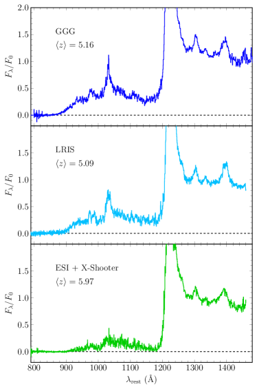
Figure 2: Composite spectra analyzed in this work. Panels are labeled with the sample name and the mean redshift of the QSOs included in the sample. The flux per unit wavelength has been normalized by the continuum flux near rest-frame 1450 Å for the GGG sample and over 1270–1380 Å for the LRIS and ESI + X-Shooter samples. Details of the Lyman continuum flux profiles are shown in Fig 6.

We created composite spectra from each of our three samples using the following procedure. We first shifted each spectrum to rest-frame wavelengths. We then divided each spectrum by its continuum flux measured over wavelengths where the flux from broad emission lines is minimal. For the GGG spectra we used the continuum flux near 1450 Å, following Worseck et al. (2014), while for LRIS, ESI, and X-Shooter we used the median flux over 1270–1380 Å. The choice of wavelength range for the continuum estimate has little impact on results because the normalization of the Lyman continuum profile is treated as a free parameter. For the LRIS, ESI, and X-Shooter spectra we corrected for residual zero-point errors by subtracting the median flux measured over a wavelength range expected to be free of transmitted flux. These wavelength ranges (750–800 Å rest frame for LRIS and 820–860 Å for ESI and X-Shooter) were verified to lie well blueward of where the fitted profiles reach zero flux (see Section 3.6). For the $z\sim 6$ data the lower wavelength bound was chosen to avoid the noisy edge of the X-Shooter VIS coverage, as well residuals from the 5577 Å skyline. The zero-point estimates for these spectra were subtracted prior to creating the composites; however, we do not require the corrections to be perfect. For the GGG sample, moreover, the wavelength coverage of the blue-side spectra does not provide a window where the zero point can be estimated safely blueward of the edge of the transmitted flux. In all cases, therefore, we include the zero point as a free parameter when fitting models to a composite. For an alternate treatment of the zero-point errors in the GGG data see Worseck et al. (2014).

Wavelength regions affected by skyline subtraction residuals were identified via peaks in the error arrays and masked. The ESI and X-Shooter spectra were also lightly median filtered using a 3-pixel sliding window to reject spurious bad pixels. Mean composite spectra were then computed in bins of 170 km s^-1 for GGG (similar to the binning used by Worseck et al. 2014) and 120 km s^-1 for the LRIS and ESI + X-Shooter data. The results are shown in Fig. 2.

In the measurements described below we use bootstrap resampling to estimate the uncertainty in $\lambda_{\rm mfp}$. In each realization, we randomly select $n_{\rm qso}$ objects from each sample, with replacement, where $n_{\rm qso}$ corresponds to the numbers in Table 1. Before creating the new composite we add a random redshift offset to each spectrum (excluding those with [C ii] 158 $\mu$m or nebular Ly$\alpha$ redshifts) drawn from a Gaussian distribution with $\sigma=180$ km s^-1(see Section 2.5). As noted by Worseck et al. (2014), we found that the redshift errors produce an uncertainty in $\lambda_{\rm mfp}$ that is small compared to the uncertainty from cosmic variance. We nevertheless include them for completeness. The bootstrap trials are also used to estimate the pixel-to-pixel errors in the flux, which we smooth using a polynomial fit over the wavelength range used to measure $\lambda_{\rm mfp}$. Additional sources of error are described in Section 3.3.

When fitting the composites we include wavelengths down to 826 Å for GGG, which is limited by the wavelength coverage of the data. For LRIS we fit down to 800 Å, while for ESI + X-Shooter we fit down to 820 Å. We note that wavelength range used to fit the composite overlaps with the wavelength range used to measure zero point offsets in the ESI and X-Shooter spectra. We find, however, that this choice does not have a significant impact on our results. The upper bound in wavelength is 910 Å for all composites, a choice we describe in Section 3.1.

3 Mean Free Path Measurements

3.1 Formalism

We measure a mean free path from the composite spectra using an approach based on the method first developed by Prochaska et al. (2009) and adapted by Worseck et al. (2014) to higher redshifts. The major change included here is to allow the ionizing opacity of the IGM to scale with the local photoionization rate. As demonstrated below, this change is necessary for extending the direct measurement method to $z\sim 6$.

The observed flux, $f_{\lambda}^{\rm obs}$, will be the mean intrinsic QSO spectral energy distribution, $f_{\lambda}^{\rm SED}$, attenuated by the effective Lyman series opacity of the foreground IGM, $\tau_{\rm eff}^{\rm Lyman}$, and the Lyman continuum effective optical depth, $\tau_{\rm eff}^{\rm LyC}$,

$$f_{\lambda}^{\rm obs}=f_{\lambda}^{\rm SED}\exp{\left(-\tau_{\rm eff}^{\rm Lyman}\right)}\exp{\left(-\tau_{\rm eff}^{\rm LyC}\right)}+f_{0}\,.$$ (1)

Here, $f_{0}$ is a zero-point correction that we include as a free parameter (see Section 2.6). We discuss the foreground Lyman series opacity in Section 3.4. The intrinsic SED blueward of the Lyman limit is modeled as a power law of the form $f_{\lambda}^{\rm SED}=f_{912}\left(\frac{\lambda}{912~{}\mbox{\small\AA}}\right)^{-\alpha_{\lambda}^{\rm ion}}$. The normalization $f_{912}$ is treated as a free parameter that incorporates the intrinsic QSO SED, any Lyman continuum attenuation directly associated with the QSOs, and any relative flux calibration error between 912 Å and the rest-frame wavelengths at which the individual QSO spectra are normalized. We adopt a nominal power-law exponent of $\alpha_{\lambda}^{\rm ion}=0.5$ (see Section 3.3). Given how rapidly $\tau_{\rm eff}^{\rm Lyman}$ and $\tau_{\rm eff}^{\rm LyC}$ evolve with wavelength, we find that our results for $\lambda_{\rm mfp}$ are highly insensitive to this choice except as it impacts our calculations for the ionizing luminosity of a QSO (see Section 3.3).

The effective Lyman continuum opacity for a photon emitted at redshift $z_{\rm qso}$ that redshifts to 912 Å at redshift $z_{912}$ will be

$$\tau_{\rm eff}^{\rm LyC}(z_{912},z_{\rm qso})=\frac{c}{H_{0}\Omega_{\rm m}^{1/2}}\left(1+z_{912}\right)^{2.75}\int_{z_{912}}^{z_{\rm qso}}\kappa_{912}(z^{\prime})\left(1+z^{\prime}\right)^{-5.25}dz^{\prime}\,,$$ (2)

where $\kappa_{912}(z)$ is the Lyman continuum opacity at 912 Å at redshift $z$ (Prochaska et al., 2009). The wavelength dependence of the ionizing absorption cross-section is approximated here as $\sigma(\lambda)\propto\lambda^{-2.75}$ following O’Meara et al. (2013) and Worseck et al. (2014).

Previous works at $z\geq 3$ have held $\kappa_{912}$ fixed when fitting a single QSO composite spectrum (Prochaska et al., 2009; Fumagalli et al., 2013; Worseck et al., 2014). The difficulty with this approach at $z>5$, however, is that $\lambda_{\rm mfp}$ may become comparable to or smaller than a typical QSO proximity zone. If the ionizing flux from a QSO decreases the opacity of the IGM in its proximity zone then this will lead to a measurement of $\lambda_{\rm mfp}$ that is biased high with respect to its value far from the QSO (see discussions in Worseck et al., 2014; D’Aloisio et al., 2018). This effect can be diminished by selecting QSOs that are relatively faint and hence have shorter proximity zones, as we have done for the LRIS sample. The measurement may still be biased, however, depending on the intrinsic value of $\lambda_{\rm mfp}$. At $z\sim 6$, moreover, $\lambda_{\rm mfp}$ is expected to be significantly shorter than the typical proximity zone of any QSO bright enough to obtain a useful spectrum.

We therefore attempt to account for the proximity effect by modeling the impact of ionizing flux from a QSO on the Lyman continuum attenuation in its vicinity. We parametrize the dependence of the opacity on the local H i ionization rate, $\Gamma$, as a power law of the form

$$\kappa_{912}=\kappa_{912}^{\rm bg}\left(\frac{\Gamma}{\Gamma_{\rm bg}}\right)^{-\xi}\,,$$ (3)

where $\kappa^{\rm bg}_{912}$ is the background opacity and $\Gamma_{\rm bg}$ is the average background photoionization rate. This form is motivated by analytic models of the IGM opacity (Miralda-Escudé et al., 2000; Furlanetto & Oh, 2005), as well as radiative transfer simulations of Lyman limit systems (McQuinn et al., 2011). These studies suggest values of $\xi\sim 2/3$ at $z>5$, which has been adopted in recent models of the Ly$\alpha$ forest opacity fluctuations at these redshifts (Davies & Furlanetto, 2016; D’Aloisio et al., 2018; Nasir & D’Aloisio, 2020). The uniform opacity model used by Worseck et al. (2014) corresponds to $\xi=0$. We discuss our priors on $\xi$ further in Section 3.5.

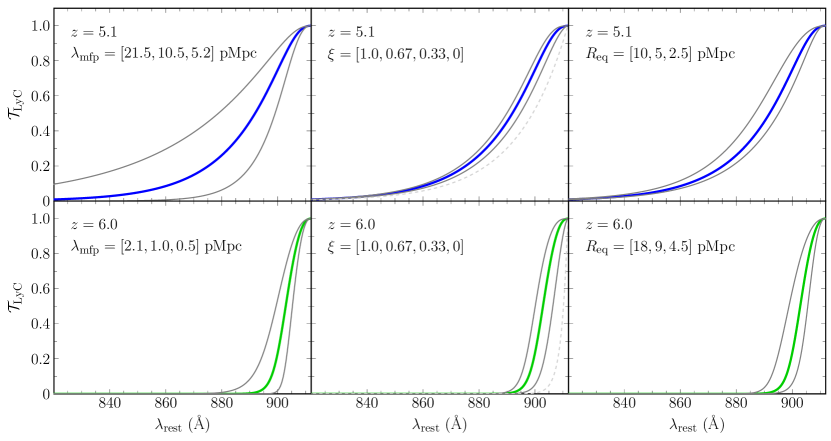
Figure 3: Examples of Lyman continuum transmission for different model parameters. At $z=5.1$ (top row), the thick lines show the fiducial model with $\lambda_{\rm mfp}=10.5$ pMpc, $\xi=0.67$, and $R_{\rm eq}=5$ pMpc. At $z=6.0$ (bottom row), the thick lines show the fiducial model with $\lambda_{\rm mfp}=1.0$ pMpc, $\xi=0.67$, and $R_{\rm eq}=9$ pMpc. The left, center, and right columns demonstrate how the transmission changes with $\lambda_{\rm mfp}$, $\xi$, and $R_{\rm eq}$, respectively. The left-to-right ordering of the parameters listed in brackets corresponds to the left-to-right ordering of the lines in each panel. In the center column, the dashed line shows the $\xi=0$ case. Note that these transmission profiles include only Lyman continuum opacity.

The local photoionization rate will be the sum of the background rate and the contribution from the QSO, which decreases with distance, giving $\Gamma=\Gamma_{\rm bg}+\Gamma_{\rm qso}(r)$. The Lyman limit opacity will therefore increase with distance from the QSO as

$$\kappa_{912}(r)=\kappa_{912}^{\rm bg}\left[1+\frac{\Gamma_{\rm qso}(r)}{\Gamma_{\rm bg}}\right]^{-\xi}\,.$$ (4)

Following Calverley et al. (2011), we characterize the ionizing luminosity of a QSO relative to the ionizing background according to the distance from the QSO, $R_{\rm eq}$, at which $\Gamma_{\rm qso}$ would be equal to $\Gamma_{\rm bg}$ in the absence of any absorption or redshifting of ionizing photons from the QSO. We note that the actual distance at which $\Gamma_{\rm qso}=\Gamma_{\rm bg}$ will tend to be less than $R_{\rm eq}$ due to absorption. Nevertheless, $R_{\rm eq}$ is a convenient parameter for helping to quantify how $\kappa_{912}$ is modified near a QSO. For a QSO with luminosity $L_{1450}$ at rest-frame 1450 Å and a broken power-law continuum of the form

$$L_{\nu}(\nu)\propto\begin{cases}\nu^{-\alpha_{\nu}^{\rm UV}},&912~{}\mbox{\AA}<\lambda<1450~{}\mbox{\AA}\\ \nu^{-\alpha_{\nu}^{\rm ion}},&\lambda<912~{}\mbox{\AA}\end{cases}$$ (5)

the luminosity at 912 Å will be $L_{912}=L_{1450}(\nu_{912}/\nu_{1450})^{-\alpha_{\nu}^{\rm UV}}$ and this distance will be

$$R_{\rm eq}=\left[\frac{L_{912}\,\sigma_{0}}{4\pi\,\Gamma_{\rm bg}\,(\alpha_{\nu}^{\rm ion}+2.75)}\right]^{1/2}\,.$$ (6)

Here, $\sigma_{0}$ is the H i ionization cross-section at 912 Å. We calculate $L_{1450}$ from the absolute magnitudes listed in Table 2. In Section 3.3 we calculate mean $R_{\rm eq}$ values for our samples and discuss constraints on $\Gamma_{\rm bg}$, $\alpha_{\nu}^{\rm UV}$, and $\alpha_{\nu}^{\rm ion}$. The ionizing flux from the QSO will be diluted geometrically and attenuated by Lyman continuum absorption, which increases with distance as $\Gamma_{\rm qso}$ decreases. We therefore solve for $\Gamma_{\rm qso}(r)$ and $\kappa_{912}(r)$ numerically under the assumption that $\kappa_{912}(r=0)=0$. Specifically, we divide the line of sight into small steps of distance $\delta r$. For the first step we assume that $\Gamma_{\rm qso}$ decreases purely geometrically, i.e.,

$$\Gamma_{\rm qso}(r=\delta r)=\Gamma_{\rm bg}\left(\frac{\delta r}{R_{\rm eq}}\right)^{-2}\,.$$ (7)

Over subsequent steps we solve for $\Gamma_{\rm qso}(r+\delta r)$ as

$$\Gamma_{\rm qso}(r+\delta r)=\Gamma_{\rm qso}(r)\left(\frac{r+\delta r}{r}\right)^{-2}e^{-\kappa_{912}(r)\delta r}\,,$$ (8)

where $\kappa_{912}(r)$ is computed using equation (4).

In principle, $L_{912}$ in equation (6) could be modified by an escape fraction, $f_{\rm esc}$ (e.g., Cristiani et al., 2016). For simplicity, however, we assume that the QSOs in our sample are roughly bimodal in terms of their escape fraction, having either $f_{\rm esc}\sim 0$ or 1, with $f_{\rm esc}$ independent of luminosity. Other than cases where there is an obvious, strong associated absorber such as DLA (see Section 2.4), we do not wish to bias our results by attempting to exclude QSOs with low $f_{\rm esc}$. Fortunately, QSOs with $f_{\rm esc}=0$ will have zero flux blueward of 912 Å. Including these objects should therefore only rescale the mean Lyman continuum profile, which will be captured by the normalization parameter, $f_{912}$. Redshift errors may cause absorption from associated high-order Lyman series lines to be blended into the composite flux below 912 Å. We mitigate this by restricting our fits to $\lambda_{\rm rest}<910$ Å, i.e., $\sim$600 km s^-1 blueward of the nominal QSO redshifts.

In total, therefore, our model for the Lyman continuum flux includes five parameters, $f_{912}$, $f_{0}$, $\kappa_{912}^{\rm bg}$, $R_{\rm eq}$, and $\xi$. The quantity we wish to obtain is the background mean free path that would be expected in the absence of the proximity effect. The mean free path is defined here to be the distance travelled by photons (emitted at a wavelength somewhat shorter than 912 Å) that would be attenuated by a factor of $1/e$ by Lyman continuum absorption. In order to calculate this quantity with the proximity effect removed, we recompute the effective Lyman continuum opacity by setting $\kappa_{912}=\kappa_{912}^{\rm bg}$ in equation (2). Given the relatively short mean free path at these redshifts, we neglect any redshift evolution of $\kappa_{912}^{\rm bg}$. We then compute $\lambda_{\rm mfp}$ as the distance between $\langle z_{\rm qso}\rangle$ and $z_{912}$ at which $\tau_{\rm eff}^{\rm LyC}(z_{912},\langle z_{\rm qso}\rangle)=1$.

Examples of our model Lyman continuum transmission ($\mathcal{T}_{\rm LyC}=e^{-\tau_{\rm eff}^{\rm LyC}}$) are shown in Fig. 3. The fiducial models at $z=5.1$ and 6.0 use $[\lambda_{\rm mfp},\xi,R_{\rm eq}]=[10.5~{}{\rm pMpc},0.67,5.0~{}{\rm pMpc}]$ and $[1.0~{}{\rm pMpc},0.67,9.0~{}{\rm pMpc}]$, respectively. The $\lambda_{\rm mfp}$ values correspond to $\log{(\kappa^{\rm bg}_{912}/{\rm cm^{-2}})}=-25.5$ ($-$24.5) at $z=5.1$ (6.0). For all models we fix $f_{912}=1$ and $f_{0}=0$. The fiducial models were chosen to be similar to those measured from the data (see Sections 3.3 and  3.6). We then show how the profile varies with $\lambda_{\rm mfp}$, $\xi$, and $R_{\rm eq}$. Changes in $\xi$ and $R_{\rm eq}$ have a wavelength (radial) dependence that is significantly different from $\lambda_{\rm mfp}$ because $\xi$ and $R_{\rm eq}$ mainly impact the transmission profile within the proximity zone. As expected, the relative importance of the proximity effect is larger at $z=6.0$, where a change of $\pm 1/3$ in $\xi$ or a factor of two change in $R_{\rm eq}$ produces a comparable change in the transmission profile as a factor of two change in $\lambda_{\rm mfp}$. Even so, these examples suggest that it is possible to measure $\lambda_{\rm mfp}$ at $z=6$ given reasonable constraints on $\xi$ and $R_{\rm eq}$, even when $R_{\rm eq}$ is a factor of ten larger than $\lambda_{\rm mfp}$. Our constraints on $\xi$ and $R_{\rm eq}$ are discussed further below.

3.2 Tests with mock spectra

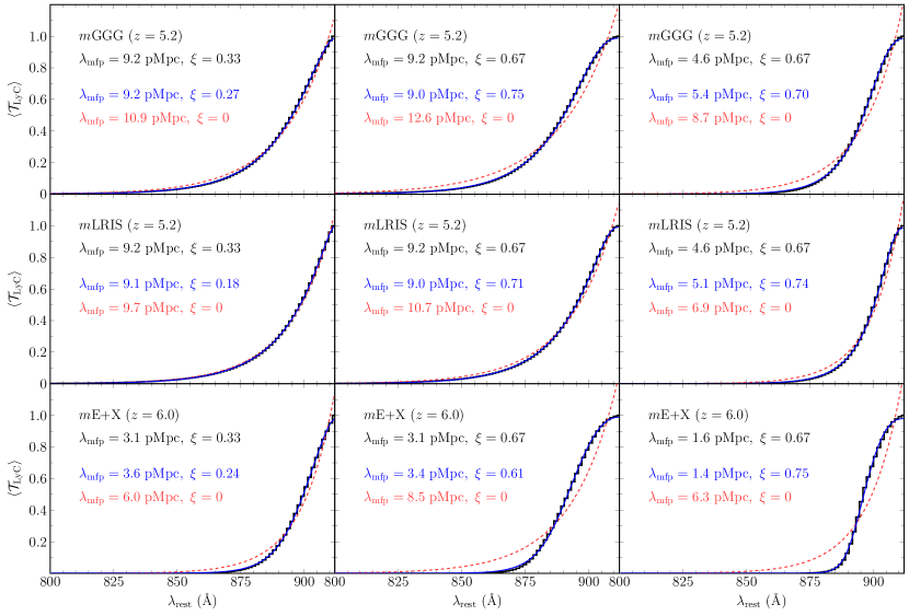
Figure 4: Fits to mock composite Lyman continuum transmission profiles. The top line in the legend in each panel gives the observed QSO sample to which the simulated QSO sample is matched in luminosity, along with the redshift. The second line gives the “true” values of $\lambda_{\rm mfp}$ and $\xi$ for that mock. Each mock spectrum (histogram) is an average of 1,000 lines of sight towards each QSO in the sample. The solid line is a fit in which both $\kappa_{\rm bg}$ (and hence $\lambda_{\rm mfp}$) are treated as free parameters, with results given in the third line of the legend. The dotted line is a fit assuming constant opacity ($\xi=0$), with results given in the fourth line. See Section 3.2 for details.

Here we investigate how well our analytic model recovers the relevant parameters from mock spectra drawn from simulations. We refer the reader to Section 4 of D’Aloisio et al. (2018) for a description of the simulations. In summary, we assign QSOs with luminosities taken from the GGG, LRIS, and ESI + X-Shooter samples to the most massive halos in a cosmological hydrodynamics simulation with box $L=200~{}h^{-1}$ Mpc and $N_{\rm gas}=N_{\rm dm}=2048^{3}$ gas and dark matter resolution elements. The hydrodynamics simulation was run with a modified version of the code of Trac & Pen (2004). The QSO halos masses range from 1.3 to $8.0\times 10^{12}~{}h^{-1}\,{\rm M_{\odot}}$. The QSO luminosities at 1450 Å rest-frame are taken from Table 2. We compute the ionizing luminosity of each QSO assuming a broken power-law of the form given by Lusso et al. (2015), which is similar to what we assume for the data (see Section 3.3).

One QSO is populated in the box at a time and we use the attenuation model of Davies & Furlanetto (2016) to compute the $\Gamma$ and $\lambda_{\rm mfp}$ fields in the box. These iterative calculations include galactic sources, spatially varying $\lambda_{\rm mfp}$  and the backreaction of $\Gamma$ on local $\lambda_{\rm mfp}$ values. The background ionization rates are $\Gamma_{\rm bg}=5\times 10^{-13}$ s^-1 and $1\times 10^{-13}$ s^-1 at $z=5.2$ and 6, respectively, which are somewhat different than the values we use when fitting the data (see below). For the $\Gamma$ and $\lambda_{\rm mfp}$ computations we use uniform grids with $64^{3}$ cells. We compute $1,000$ transmission profiles along random sight lines emanating from each QSO in a given sample. We then construct $1,000$ mock composite spectra by averaging over the QSOs in the sample.

Mock transmission profiles are generated for different combinations of $\lambda_{\rm mfp}$ and $\xi$ at $z=5.2$ and 6.0. At $z=5.2$ we consider a “long” mean free path model with $\lambda_{\rm mfp}=9.2$ pMpc (40 comoving $h^{-1}\,$Mpc) with either $\xi=0.33$ or $0.67$, and a “short” mean free path model with $\lambda_{\rm mfp}=4.6$ pMpc (20 comoving $h^{-1}\,$Mpc) and $\xi=0.67$. At $z=6.0$ we use $\lambda_{\rm mfp}=3.1$ pMpc (15 comoving $h^{-1}\,$Mpc) with either $\xi=0.33$ or $0.67$, and $\lambda_{\rm mfp}=1.6$ pMpc (8 comoving $h^{-1}\,$Mpc) with $\xi=0.67$.

We test how well our fitting approach recovers the “true" $\lambda_{\rm mfp}$ and $\xi$ values by fitting our model to the mock composite spectra. We compute $R_{\rm eq}$ for each QSO using the $\Gamma_{\rm bg}$ values quoted above. For consistency, we use the same QSO SED that was used to compute the ionizing luminosities for the mock sample. The mean $R_{\rm eq}$ values are 7.4, 3.5, and 16.9 pMpc for the mock GGG, LRIS, and ESI + X-Shooter samples, respectively, which we adopt when fitting the models. These values are somewhat larger than the values we compute for the data (see Section 3.3), mainly due to the difference in $\Gamma_{\rm bg}$. Our fits to the mock composites have three free parameters: $\kappa^{bg}_{912}$, $\xi$, and $f_{912}$. For comparison, we also fit a constant opacity model that ignores the QSO proximity effect ($\xi=0$). We employ a chi-squared approach assuming equal variance in each wavelength bin. The mocks do not include foreground Lyman series absorption or variations due to intrinsic QSO SEDs. They therefore allow us to determine how well the $\lambda_{\rm mfp}$ and $\xi$ values are recovered under ideal circumstances.

Fits to the mock transmission profiles are shown in Fig. 4. In each case where we include the proximity effect in the fit we recover the correct $\lambda_{\rm mfp}$ to within 17%. This is true even in the “short” ($\lambda_{\rm mfp}=1.6$ pMpc) case at $z=6$, where $R_{\rm eq}$ is a factor of ten larger than $\lambda_{\rm mfp}$. We also recover the correct $\xi$ to within $\sim$0.1 in all cases except the $\lambda_{\rm mfp}=9.2$ pMpc, $\xi=0.33$ case with the mock LRIS composite, where the impact of the proximity effect is weakest. In contrast, ignoring the proximity effect can produce a significant overestimate of the mean free path (and overestimates of the normalization, a fact that may be evident when fitting high-$S/N$ composites). For $\lambda_{\rm mfp}=4.6$ pMpc and $\xi=0.67$, the $\lambda_{\rm mfp}$ values returned for the LRIS and GGG mocks are too large by factors of 1.5 and 1.9, respectively. This suggests that accounting for the proximity effect may be necessary even for fainter QSOs, depending on the true value of $\lambda_{\rm mfp}$. Errors for the constant opacity model are largest at $z=6$, with $\lambda_{\rm mfp}$ overestimated by up by factors of two to four.

In summary, we find that reasonable estimates of $\lambda_{\rm mfp}$ can be obtained even when the mean free path is much shorter than the proximity zone size provided that the proximity effect is taken into account. Fitting a constant opacity model to Lyman continuum profiles at $z>5$, in contrast, can lead to significant overestimates of the mean free path, even for samples of relatively faint QSOs. In principle, at least, it is also possible to recover the scaling of Lyman continuum opacity with local ionization rate. Directly constraining $\xi$ requires extremely good data, however, a point we return to below.

An important caveat is that the simulations on which we validated our technique for simultaneously fitting $\lambda_{\rm mfp}$ and $\xi$ do not include dynamical effects that are especially relevant if reionization ended near $z=6$. Park et al. (2016) and D’Aloisio et al. (2020) found that impulsive changes to the UVB (e.g. reionization or a QSO turning on suddenly) shape the density structure of the IGM over $\Delta t\sim 100$ Myr through the interplay between self-shielding and hydrodynamic response of the gas to photoheating. One implication raised by D’Aloisio et al. (2020) is that the dependence of $\lambda_{\rm mfp}$ on $\Gamma$ may be more complex than can be captured with a universal power law. The simulations also assume an infinite QSO lifetime. If the QSOs are much younger than the $\sim 100$ Myr relaxation timescale of the optically thick absorbers that set $\lambda_{\rm mfp}$, another distinct possibility is that the local mean free paths have not had sufficient time to respond to the enhanced UV intensities. In this case, the proximity effect would be less apparent in the measurements of $\lambda_{\rm mfp}$.

3.3 $R_{\rm eq}$ values for observed QSOs

The $R_{\rm eq}$ estimates for our QSOs are derived from observational constraints on the metagalactic hydrogen ionization rate and the mean SED of high-redshift QSOs. Similar to previous works (e.g., Becker & Bolton, 2013), we estimate $\Gamma_{\rm bg}$ based on the mean intergalactic Ly$\alpha$ transmission at these redshifts. Our nominal evolution in the mean Ly$\alpha$ transmission, described in Section 3.4, corresponds to $\langle\mathcal{T}_{\rm Ly\alpha}\rangle=0.14$ at $z=5.1$ and $\langle\mathcal{T}_{\rm Ly\alpha}\rangle=0.0072$ at $z=6.0$. These values are based on measurements made from QSO spectra well outside the proximity zone (see below). We use a hydrodynamical simulation to translate these $\langle\mathcal{T}_{\rm Ly\alpha}\rangle$ values into $\Gamma_{\rm bg}$ estimates by rescaling the simulated UV background such that the mean Ly$\alpha$ transmission of the simulation box matches observations. Specifically, we use the 40 $h^{-1}\,$Mpc box with $2\times 2048^{3}$ particles (40-2048) from the Sherwood simulation suite (Bolton et al., 2017), whose IGM temperatures over $5<z<6$ are broadly consistent with existing measurements (Bolton et al., 2012; Boera et al., 2019; Walther et al., 2019; Gaikwad et al., 2020). This procedure yields $\Gamma_{\rm bg}\simeq 7\times 10^{-13}$ s^-1 and $3\times 10^{-13}$ s^-1 at $z=5.1$ and 6.0, respectively. The uncertainties affecting $\Gamma_{\rm bg}$, including those related to $\langle\mathcal{T}_{\rm Ly\alpha}\rangle$, the temperature-density relation, and numerical effects, are similar to those in Becker & Bolton (2013). We therefore adopt a similar overall error on our $\Gamma_{\rm bg}$ estimates, namely $\pm$0.15 dex. For the QSO SED in equation (5) we adopt $\alpha_{\nu}^{\rm UV}=0.6\pm 0.1$ and $\alpha_{\nu}^{\rm ion}=1.5\pm 0.3$ ($\alpha_{\lambda}^{\rm ion}=0.5\pm 0.3$). The choice of $\alpha_{\nu}^{\rm UV}$ is taken from fits to composite QSO spectra by Lusso et al. (2015), and is generally consistent with other similar works (Vanden Berk et al., 2001; Shull et al., 2012; Stevans et al., 2014). Here we adopt a larger error than found by Lusso et al. (2015) in order to allow for greater sample variance. Our choice of $\alpha_{\nu}^{\rm ion}$ is broadly consistent with fits to composite spectra from Telfer et al. (2002), Stevans et al. (2014), and Lusso et al. (2015) (though see Scott et al. 2004, who find a harder ionizing slope for low-redshift AGN). For the above parameters and the $M_{1450}$ values listed in Table 2 we calculate mean $R_{\rm eq}$ values of 6.4, 3.0, and 11.1 pMpc for the GGG, LRIS, and ESI + X-Shooter samples, respectively.

For each bootstrap composite that is used to estimate the uncertainty in $\lambda_{\rm mfp}$ (see Section 2.6) we randomly sample the above error distributions for $\Gamma_{\rm bg}$, $\alpha_{\nu}^{\rm UV}$, and $\alpha_{\nu}^{\rm ion}$ and propagate these into the estimates of $R_{\rm eq}$ for each object. We then recompute the mean $R_{\rm eq}$ based on the objects in that bootstrap sample. The same value of $\alpha_{\nu}^{\rm ion}$ is used to model the Lyman continuum transmission profile for a given bootstrap trial. When fitting the GGG and LRIS profiles simultaneously, the same random realizations of $\Gamma_{\rm bg}$ and the QSO spectral indices are applied to both data sets. For reference, the 68% (95%) ranges of the mean $R_{\rm eq}$ values from the bootstrap trials are 5.4–7.8 (4.5–9.3) pMpc, 2.5–3.6 (2.1–4.3) pMpc, and 10.3–15.1 (8.6–18.2) pMpc for the GGG, LRIS, and ESI + X-Shooter samples, respectively.

3.4 Foreground Lyman series transmission

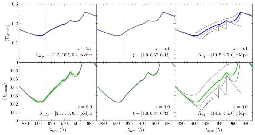
Figure 5: Examples of Lyman series transmission for different model parameters. At $z=5.1$ (top row), the thick lines show the fiducial model with $\lambda_{\rm mfp}=10.5$ pMpc, $\xi=0.67$, and $R_{\rm eq}=5$ pMpc. At $z=6.0$ (bottom row), the thick lines show the fiducial model with $\lambda_{\rm mfp}=1.0$ pMpc, $\xi=0.67$, and $R_{\rm eq}=9$ pMpc. The left, center, and right columns demonstrate how the transmission changes with $\lambda_{\rm mfp}$, $\xi$, and $R_{\rm eq}$, respectively. The left-to-right ordering of the parameters listed in brackets corresponds to the top-to-bottom ordering of the lines in each panel. In the right column, the jagged line corresponds to the no proximity effect ($R_{\rm eq}=0$) case. Vertical dotted lines mark the Lyman limit. Note that the model parameters only impact the change in transmission due to the proximity effect and do not self-consistently modify the baseline opacity (see Section 3.4).

The Lyman series opacity at an observed wavelength $\lambda_{\rm obs}<(912~{}\mbox{\AA})(1+z_{\rm qso})$ will include foreground contributions from all Lyman series lines,

$$\tau_{\rm eff}^{\rm Lyman}(\lambda_{\rm obs})=\sum_{j}\tau_{\rm eff}^{j}(z_{j})\,$$ (9)

where $\tau_{\rm eff}^{j}(z_{j})$ is the effective opacity of transition $j$ at redshift $z_{j}$, $(1+z_{j})\lambda_{j}=\lambda_{\rm obs}$, and $\lambda_{j}$ is the rest-frame wavelength of transition $j$. We compute $\tau_{\rm eff}^{\rm Lyman}$ using the 40-2048 Sherwood simulation described above. The simulation outputs are spaced in redshift intervals of $\Delta z=0.1$, with 5000 lines of sight drawn from each output. At each simulation redshift we first compute baseline Ly$\alpha$ optical depths by rescaling the native simulated Ly$\alpha$ optical depths to reproduce the observed mean IGM Ly$\alpha$ transmission. The optical depths for 38 higher-order Lyman line are then computed as $\tau^{j}/\tau^{\alpha}=(f_{j}\lambda_{j})/(f_{\alpha}\lambda_{\alpha})$, where $f$ here is the oscillator strength. The mean Ly$\alpha$ transmission, $\langle\mathcal{T}_{\rm Ly\alpha}\rangle=e^{-\tau_{\rm eff}^{\alpha}}$, is taken from Becker et al. (2013) at $z\leq 4$ and interpolated between the values of Bosman et al. (2018) at $z\geq 5.2$. Following Boera et al. (2019), we bridge between these two sets of measurements with a power law of the form $\tau_{\rm eff}^{\alpha}(z)=1.56\left[(1+z)/5.75\right]^{4.0}$ over $4.0<z<5.2$. For reference, our adopted $\langle\mathcal{T}_{\rm Ly\alpha}\rangle$ values at $z=3.5,4.0$, 4.5, 5.0, 5.5 and 6.0 are 0.54, 0.41, 0.27, 0.16, 0.067, and 0.0072, respectively.

We note that we are computing the Lyman series transmission from an optically thin simulation that does not include elements such as galactic outflows and self-shielded gas that may modify the neutral hydrogen density distribution, and hence impact the ratio of $\tau_{\rm eff}^{j}/\tau_{\alpha}$ for high-order lines. The numerical resolution of the simulations may also have an effect. We tested the numerical resolution using the 40-1024 run from the Sherwood suite, which also uses a 40 $h^{-1}\,$Mpc box but is a factor of eight lower in mass resolution than our fiducial 40-2048 run. Using the lower resolution run increased the total Lyman series transmission over 890$-$912 Å in the rest frame by 2% (10%) for QSOs at $z=5.1$ (6.0). We tested the impact of galaxy physics using the 40-1024-ps13 runs from Bolton et al. (2017), which include a subgrid implementation of star formation and galactic outflows from Puchwein & Springel (2013). These decreased the transmission relative to the 40-1024 run by 4% ($\sim$3%) at $z=5.1$ (6.0). We also tested the impact of self-shielding using a version of the 40-1024-ps13 run in which self-shielding was added in post-processing following Rahmati et al. (2013) at $z<5$ and Chardin et al. (2018) at $z>5$. This decreased the mean transmission by a further 3% (2%) at $z=5.1$ (6.0). Fortunately, in all cases the effect was mainly to rescale the transmission below 912 Å and not to change the shape of the profile in a way that would significantly impact our $\lambda_{\rm mfp}$ measurements. These effects may nevertheless need to be considered in future works.

An additional factor here is the QSO proximity effect. We include the proximity effect for each Lyman series line following the same numerical approach used to compute the Lyman continuum opacities. For a given combination of $\kappa^{\rm bg}_{912}$ and $\xi$ we compute $\tau_{\rm eff}^{j}$ as a function of wavelength over a grid in QSO redshift and $R_{\rm eq}$, interpolating between simulation redshifts as needed. For each composite or bootstrap sample we then compute $\tau_{\rm eff}^{\rm Lyman}(\lambda_{\rm obs})$ individually for each QSO using equation (9). We then compute the transmission as $\mathcal{T}_{\rm Lyman}=\exp{\left(-\tau_{\rm eff}^{\rm Lyman}\right)}$, and average the transmission over all lines of sight.

In Fig. 5 we plot the Lyman series absorption for different combinations of $\lambda_{\rm mfp}$, $\xi$, and $R_{\rm eq}$ at $z=5.1$ and 6.0. At $z=5.1$ the transmission is not strongly affected by $\lambda_{\rm mfp}$ or $\xi$ because the decrease in $\Gamma_{\rm tot}$ with distance from the QSO is mainly driven by geometric dilution. Including the proximity effect increases $\langle\mathcal{T}_{\rm Lyman}\rangle$ by a factor of $\sim$1.3 at rest-frame 912 Å for $R_{\rm eq}=5$ pMpc, similar to the mean value in the GGG sample. It also modifies the shape of the Lyman series transmission with respect to the no proximity effect ($R_{\rm eq}=0$) case. At $z=6.0$ the effect is even larger, with $\langle\mathcal{T}_{\rm Lyman}\rangle$ increasing at 912 Å by a factor of 2.5 for $R_{\rm eq}=5$ pMpc, similar to the mean value for the ESI + X-Shooter sample. There is also a greater dependence on $\lambda_{\rm mfp}$ and $\xi$. We find, however, that our final results are not highly dependent on the choice of $\lambda_{\rm mfp}$ and $\xi$ used for the Lyman series transmission. When computing $\langle\mathcal{T}_{\rm Lyman}\rangle$, therefore, we hold these parameters fixed at the nominal values shown in Fig. 5, which are comparable to our best-fit results.

3.5 Priors on $\xi$

The scaling of $\kappa_{912}$ with $\Gamma$ is highly uncertain, especially at the high redshifts that are relevant for this study. From a theoretical viewpoint, the value of $\xi$ is tied to the shape of the gas density distribution function near the self-shielding threshold. Adopting the Miralda-Escudé et al. (2000) model of IGM opacity, and assuming that the density profile of a typical self-shielding absorber is isothermal, it can be shown that $\kappa_{912}\propto\Gamma^{-2/3}$, i.e. $\xi=2/3$ (Furlanetto & Oh, 2005; McQuinn et al., 2011). Indeed, this value has been adopted in recent models of the fluctuating UVB at $z>5$ (e.g. Davies & Furlanetto, 2016; D’Aloisio et al., 2018; Nasir & D’Aloisio, 2020). Using radiative transfer simulations of self-shielding systems, McQuinn et al. (2011) found an even steeper scaling at $z=6$ with $\xi\approx 0.75$ (see their Fig. 4 and footnote 8 of D’Aloisio et al. 2018). It should be noted, however, that the radiative transfer in their study was applied in post processing to absorbers extracted from hydrodynamic simulations. This approach misses the effect of the UVB on the density structure of the absorbers.

More recently, D’Aloisio et al. (2020) used fully coupled radiation hydrodynamics simulations to study self-shielding systems (see also Park et al. 2016). Their findings suggest a more complex dependence of $\kappa_{912}$ on $\Gamma$ owing to the interplay between self-shielding and the hydrodynamic response of the gas to photoheating, which occurs on a time scale of hundreds of Myr. We can nonetheless examine their gas density distribution functions in an attempt to gain insight into $\xi$ (see their Fig. 5). At densities well above self-shielding, the probability distribution of $\Delta$ is reasonably approximated by $P\propto\Delta^{-1.8}$, where $\Delta$ is the gas density in units of the cosmic mean. Applying the analytic arguments of Furlanetto & Oh (2005) and McQuinn et al. (2011) yields a milder scaling of $\xi\approx 0.33$. This would be the scaling for a short time after a bright source turned on suddenly, before the gas had time to react to the impulse. We note, however, some important caveats which suggest that $\xi$ may be larger than this. First, the $P(\Delta)$ of D’Aloisio et al. (2020) are generally not well-described by a power law near self-shielding. Indeed, $\Delta^{3}P$ appears to flatten at densities closer to self-shielding, implying a stronger dependence of $\kappa_{912}$ on $\Gamma$. Secondly, the dependence would likely evolve as the density structure of the gas readjusted to the changing UVB. Based on these considerations, we argue here that $\xi=0.33$ may serve as an approximate lower limit. On the other hand, $\xi=1$ is the scaling for the case of a uniform IGM in photoionization equilibrium. This limit is approached if the opacity is dominated by diffuse gas near the mean density, rather than over-dense peaks. In our fits we adopt a nominal value of $\xi=0.67$ and a range $\xi=0.33$–1.0 with a flat prior from which we randomly sample when performing bootstrap trials. We also perform fits with $\xi$ fixed to 0.33, 0.67, and 1.0.

In principle, one can measure $\xi$ directly from the data. Even with good constraints on $R_{\rm eq}$ this is difficult, however, because at $z=5.1$ the dependence of the transmitted flux on $\xi$ is relatively weak unless the mean free path is short (Fig. 3), while at $z=6.0$ the data are too noisy to distinguish between variations in $\lambda_{\rm mfp}$ and $\xi$. In a joint fit to the GGG and LRIS data we find $\xi=0.56$, consistent with theoretical expectations, but with a 68% (95%) confidence range of 0.20 to 1.20 (-0.06 to 2.28). Much of this parameter space is strongly disfavored on theoretical grounds, as described above. The choice of $\xi$ ultimately has little impact at $z=5.1$. Setting $\xi=0.33$ (1.0) increases (decreases) our nominal result by 8% (6%). The impact of $\xi$ is more significant at $z=6.0$, where the proximity effect is more pronounced. There, setting $\xi=0.33$ (1.0) increases (decreases) our nominal result by 69% (68%). This represents a substantial portion of our error budget at $z=6.0$. In future works it may be possible to better constrain $\xi$ directly from the data.

3.6 Fits to the data

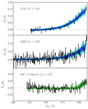
Figure 6: Fits to the data. The histogram in each panel shows the observed flux blueward of the Lyman limit for the sample indicated, normalized as in Fig. 2. Solid lines show the best-fitting model profiles, which for GGG and LRIS is a simultaneous fit to both data sets. Dark and light shaded regions show the 68% and 95% intervals, respectively, spanned by fits to the bootstrap trials.

At $z=5.1$ we fit the GGG and LRIS composites individually as well as jointly. For our nominal results we use $\xi=0.67$, as noted above, and hold the mean $R_{\rm eq}$ for each composite fixed to the values given in Section 3.3. We also include the foreground Lyman series transmission described in Section 3.4. We then fit for $\kappa_{912}^{\rm bg}$, which is used to calculate $\lambda_{\rm mfp}$, along with $f_{912}$ and $f_{0}$ separately for each composite. In the bootstrap trials we draw $\xi$ randomly from the flat distribution over $[0.3,1.0]$ while the mean $R_{\rm eq}$ is varied according to the procedure outlined above. From the individual fits we obtain $\lambda_{\rm mfp}=8.85^{+1.63}_{-1.31}$ pMpc (68% confidence intervals assuming a flat prior on $\xi$) from the GGG data and $11.64^{+4.12}_{-3.63}$ pMpc from the LRIS data. The results are thus highly consistent with one another within the errors. From the joint fit we obtain $\lambda_{\rm mfp}=9.09^{+1.62}_{-1.28}$ pMpc, which we adopt as our nominal result at $z=5.1$. At $z=6.0$ we measure $\lambda_{\rm mfp}=0.75^{+0.65}_{-0.45}$ pMpc. The nominal fits along with the ranges spanned by bootstrap trials are shown in Fig. 6. The cumulative probability density functions for $\lambda_{\rm mfp}$ at the two redshifts are shown in Fig. 7. The main results are summarized in Table 3, where we also give results for fixed values of $\xi$.

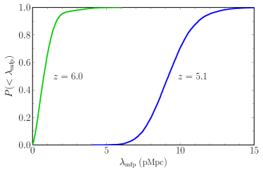
Figure 7: Cumulative probability distribution function from bootstrap fits to $\lambda_{\rm mfp}$ at $z=5.1$ (right curve) and 6.0 (left curve).

Table 3: Mean free path results

$z$	$\xi$	$\lambda_{\rm mfp}$	68% range	95% range
5.1	[0.33,1.0]	9.09	7.81–10.71	6.58–12.66
	0.33	10.06	8.83–11.57	7.78–13.37
	0.67	9.09	7.88–10.57	6.77–12.32
	1.0	8.34	7.13–9.82	6.00–11.55
6.0	[0.33,1.0]	0.75	0.30–1.40	0.07–2.67
	0.33	1.47	0.91–2.02	0.32–3.41
	0.67	0.75	0.37–1.36	0.10–2.60
	1.0	0.38	0.17–0.93	0.04–2.21

For each redshift, the first row gives the results for $\lambda_{\rm mfp}$ assuming a nominal value of $\xi=0.67$ and a flat prior over $\xi=[0.33,1.0]$. Subsequent rows give results with $\xi$ fixed.

Our value of $\lambda_{\rm mfp}$ at $z=5.1$ is consistent with the results from Worseck et al. (2014). This suggests that $\lambda_{\rm mfp}$ at this redshift is large enough that the impact of the QSO proximity effect is relatively modest, even for the brighter GGG sample where $\langle R_{\rm eq}\rangle\simeq 0.7\lambda_{\rm mfp}$. Indeed, if we neglect the proximity effect by setting $\xi=0$ and $R_{\rm eq}=0$ for both the Lyman continuum opacity and the foreground Lyman series, emulating the approach of Worseck et al. (2014), our result for $\lambda_{\rm mfp}$ increases by only 12% for the GGG composite and remains essentially unchanged for the LRIS composite. This is somewhat less than the bias found with mock spectra in Section 3.2 because the errors in the Lyman continuum modeling are partially offset by errors in the Lyman series modeling. The difference increases to 28% for the GGG sample if we include the proximity effect in the foreground Lyman series transmission but not in the Lyman continuum, a scenario closer to Figure 3, where accurate modeling of the Lyman series is assumed.

At $z=6.0$, in contrast, the mean value of $R_{\rm eq}$ is a factor of 15 larger than our value of $\lambda_{\rm mfp}$, making it critical to take the proximity effect into account. In this case, fully neglecting the proximity effect increases our $\lambda_{\rm mfp}$ measurement by a factor of 2.9 above our nominal $\xi=0.67$ value. If we attempt to emulate the mock trials by including the proximity effect in the Lyman series absorption but not in the Lyman continuum then our result for $\lambda_{\rm mfp}$ increases by a factor of 3.6. This is consistent with the bias expected from the mock trials in Section 3.2, and emphasizes the importance of properly accounting for the proximity effect at $z\sim 6$.

In Fig. 8 we plot our $\lambda_{\rm mfp}$ values as a function of redshift, along with measurements from the literature (Prochaska et al., 2009; Fumagalli et al., 2013; O’Meara et al., 2013; Worseck et al., 2014; Lusso et al., 2018). The Lusso et al. (2018) value at $z=2.44$ is their fit to the data from O’Meara et al. (2013). Lusso et al. (2018) find somewhat lower values of $\lambda_{\rm mfp}$ at $z\sim 2$ towards QSO pairs, potentially due to an increased incidence of optically thick absorbers in pair environments. We note that Romano et al. (2019) measured the mean free path towards QSOs at $z\sim 4$. They find values that are $\sim$10–20% higher than those of Prochaska et al. (2009) and Worseck et al. (2014) over the same redshifts. In trials using the two lower-redshift GGG composites from Worseck et al. (2014) we found that this discrepancy is well explained by the lack of foreground Lyman series absorption in the Romano et al. (2019) analysis. Worseck et al. (2014) fit a power law of the form $\lambda_{\rm mfp}(z)\propto(1+z)^{-5.4}$ over $2.44<z<5.16$ (dotted line in Fig. 8). Extrapolating this fit out to $z=6$ overshoots our nominal ESI + X-Shooter measurement by a factor of six, and is excluded by the data with $>$99.99% confidence. We therefore find strong evidence that the evolution of $\lambda_{\rm mfp}(z)$ with redshift steepens at $z\gtrsim 5$. This steepening is broadly consistent with the results of Songaila & Cowie (2010) based on their measurements of discrete Lyman limit absorbers towards QSOs over $5<z<6$.

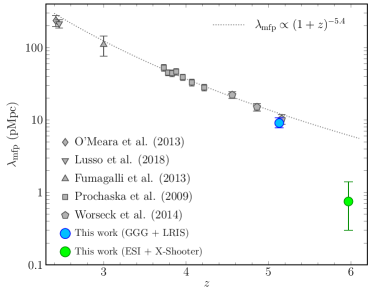
Figure 8: Direct measurements of $\lambda_{\rm mfp}$ from this work and the literature. Results from O’Meara et al. (2013) and Lusso et al. (2018) have been offset slightly in redshift for clarity. The dotted line shows the power-law fit to $\lambda_{\rm mfp}(z)$ over $2.44<z<5.16$ from Worseck et al. (2014), extrapolated out to $z=6$.

4 Discussion

4.1 Implications for reionization

Our measurements are consistent with a low value of $\lambda_{\rm mfp}$ at $z=6$ and a rapid increase from $z=6$ to 5. Taken at face value, perhaps the most interesting possibility is that this evolution is tied to the end of reionization. In Fig. 9 we compare our measurements to predictions for $\lambda_{\rm mfp}(z)$ from different reionization models. We begin with the simplistic models in D’Aloisio et al. (2020), which employ results from a suite of radiative hydrodynamics simulations of the ionizing photon sinks at $z>5$. The dotted curve shows a model in which reionization ended long before $z=6$ such that the IGM has had sufficient time to relax hydrodynamically. This model predicts a redshift evolution of $\lambda_{\rm mfp}$$\propto(1+z)^{-5.4}$ and a $\lambda_{\rm mfp}$($z=6$) that is a factor of $\sim$7 longer than our measurement. It is worth noting that this model assumes only the $\Lambda$CDM cosmology and a constant UVB intensity; yet it yields a redshift evolution for $\lambda_{\rm mfp}$ that is identical to the empirical fit of Worseck et al. (2014). The fully relaxed model is inconsistent with our $z=6.0$ measurement at the 99.9% level ($P(<\lambda_{\rm mfp})=0.999$). For comparison, the solid curves show the “rapid” and “gradual” reionization models of D’Aloisio et al. (2020) wherein reionization is 50% complete at $z=7.3$ and 9.1, respectively, and ends at $z=6$. Although $\lambda_{\rm mfp}$ at $z=6$ is lower than in the fully relaxed models, the data are still inconsistent at the 98–99% confidence levels.

It is also possible that reionization ended later than $z=6$, a scenario that has been proposed recently to explain the large scatter in the $z>5$ Ly$\alpha$ forest opacity (Kulkarni et al., 2019; Keating et al., 2020a, b; Nasir & D’Aloisio, 2020; Choudhury et al., 2020; Qin et al., 2021). The dashed curves in Fig. 9 show the “Low $\tau_{\rm CMB}$” and “Hot Low $\tau_{\rm CMB}$” models of Keating et al. (2020b), wherein reionization is 50% complete at $z\simeq 6.7$ and ends at $z\simeq 5.3$. In these models the IGM at $z=6.0$ is still $\sim$20% neutral. We also plot their "High $\tau_{\rm CMB}$” model wherein reionization ends at the same redshift but is 50% complete at $z\simeq 8.4$. In this model the IGM at $z=6.0$ is $\sim$8% neutral. The High $\tau_{\rm CMB}$ model is excluded at the 99% level. The Low $\tau_{\rm CMB}$ models are more consistent with our measurement at $z=6.0$, although the data still prefer a lower $\lambda_{\rm mfp}$ at the 97% confidence level.

We note that $\lambda_{\rm mfp}$ evolves rapidly near $z=6$ in all of these reionization models, and that they therefore become more consistent with the data if they are shifted slightly in redshift. For example, shifting the models by $\Delta z=-0.2$ decreases $P(<\lambda_{\rm mfp})$ at $z=6.0$ to 0.97 for the D’Aloisio et al. (2020) “rapid” model and 0.86 for the Keating et al. (2020b) Low $\tau_{\rm CMB}$ model. The low value of $\lambda_{\rm mfp}$ we measure at $z=6.0$ may therefore suggest that reionization occurs even later than these models propose.

We further note that the tension with existing models may be reduced if $\xi$ is near the low end of our adopted range. Our nominal $\lambda_{\rm mfp}$ value at $z=6.0$ is a factor of two higher for $\xi=0.33$ than for $\xi=0.67$ (see Table 3), a result that comes from attributing less of the transmission in Figure 6 to the proximity effect. Moreover, $P(<\lambda_{\rm mfp})$ for the Low $\tau_{\rm CMB}$ model at $z=6.0$ decreases to 0.91 when we hold $\xi$ fixed to 0.33. It is possible, therefore, that reconciling the reionization history with our measurements of $\lambda_{\rm mfp}$ may require the ionizing sinks near $z\sim 6$ to be less sensitive to photoionization effects than some models assume (for further discussion, see D’Aloisio et al., 2020).

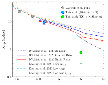
Figure 9: Measurements of $\lambda_{\rm mfp}$ from this work (circles) and Worseck et al. (2014) (pentagons), along with $\lambda_{\rm mfp}(z)$ relations from simulations. Dotted and solid lines are from D’Aloisio et al. (2020). The dotted line shows the expected evolution if the IGM reionized early enough that the absorbers have had time to fully relax hydrodynamically by $z=6$. Blue (upper) and red (lower)solid lines show their “gradual” and ”rapid" reionization models wherein reionization is 50% complete at $z=9.1$ and 7.3, respectively, and complete by $z=6$. Dashed lines are from Keating et al. (2020b). The orange (upper) line shows their "High $\tau_{\rm CMB}$” wherein reionization is 50% complete near $z\simeq 8.4$ and ends near $z\simeq 5.3$. The cyan (middle at $z<5.5$) and red (lower at $z<5.5$) dashed lines show their “Low $\tau_{\rm CMB}$” models wherein reionization still ends $z\simeq 5.3$ but is 50% complete at $z\simeq 6.7$.

4.2 Ionizing emissivity

We can use our estimates of $\Gamma_{\rm bg}$ and $\lambda_{\rm mfp}$ to infer the ionizing emissivity at $z=5$–6. Here we use the local source approximation, which neglects the redshifting of ionizing photons (e.g., Schirber & Bullock, 2003; Kuhlen & Faucher-Giguère, 2012). This is a reasonable choice given the short mean free path at $z>5$ (e.g., Becker & Bolton, 2013). Under this approximation the comoving ionizing emissivity is given by

$$\dot{N}_{\rm ion}(z)\approx\frac{1}{(1+z)^{3}}\frac{\Gamma_{\rm bg}(z)}{\sigma_{912}\lambda_{\rm mfp}(z)}\frac{(\alpha_{\rm bg}+2.75)}{\alpha_{\rm s}}\,.$$ (10)

Here, $\alpha_{\rm s}$ is the slope of the ionizing spectrum of the sources ($f_{\nu}^{\rm s}\propto\nu^{-\alpha_{\rm s}}$), and $\alpha_{\rm bg}$ is the slope of the ionizing background after filtering through the IGM. If the column density distribution of H i absorbers producing most of the Lyman continuun opacity is a power law of the form $f(N_{\rm H\,I})\propto N_{\rm H\,I}^{-\beta_{N}}$, then $\alpha_{\rm bg}=\alpha_{\rm s}-2.75(\beta_{N}-1)$. Following Becker & Bolton (2013) we adopt $\alpha_{\rm s}=2.0$ as a reasonable match to models of metal-poor star-forming galaxies, and $\beta_{N}=1.3$. Applying our $\Gamma_{\rm bg}$ and $\lambda_{\rm mfp}$ results then gives $\log{\dot{N}_{\rm ion}(z=5.1)}=0.00^{+0.16(0.32)}_{-0.17(0.33)}$ and $\log{\dot{N}_{\rm ion}(z=6.0)}=0.54^{+0.43(1.08)}_{-0.31(0.62)}$, where $\dot{N}_{\rm ion}$ is in units of $10^{51}~{}{\rm photons~{}s^{-1}~{}(comoving~{}Mpc)^{-3}}$ and the errors are 68% (95%) confidence intervals. At $z=5.1$ the errors in $\dot{N}_{\rm ion}$ are dominated by uncertainties in $\Gamma_{\rm bg}$, whereas at $z=6.0$ they are dominated by uncertainties in $\lambda_{\rm mfp}$.

The results at $z=5.1$ are similar to the values of $\dot{N}_{\rm ion}$ over $2.4<z<4.75$ found by Becker & Bolton (2013), and suggest that the ionizing emissivity over $2<z<5$ may change relatively little over this period even as the source populations of star-forming galaxies and AGN evolve considerably. In contrast, although the errors are large and we have ignored possible fluctuations in the ionizing background, the emissivity at $z=6.0$ is potentially significantly higher. If confirmed, this would suggest that the mean production efficiency and/or escape fraction of ionizing photons is higher for sources at $z\gtrsim 6$ than for sources at lower redshifts. The nominal value of $\dot{N}_{\rm ion}$ at $z=6.0$ corresponds to $\sim$17 ionizing photons per hydrogen atom per Gyr, a rate that may help explain how reionization could have been completed in only a few hundred Myr.

4.3 Caveats and future work

Finally, we note that this work has some limitations. Our measurement at $z=6.0$ is based on a relatively small sample of 13 QSOs, and within this sample there are clearly outliers in terms of Lyman continuum transmission. The spectrum of SDSS J0836$+$0054, for example, shows discrete transmission peaks down to rest-frame 870 Å (i.e., 22 pMpc from the QSO), whereas none of the other $z\sim 6$ objects shows obvious transmission below 900 Å. While a skewed distribution of free paths along individual lines of sight is expected (e.g., Romano et al., 2019), and while this particular QSO is the brightest (and lowest-redshift) one in our ESI + X-Shooter sample, a larger sample at $z\sim 6$ would help to characterize the spatial variations in ionizing opacity near the end of reionization. Given the rapid increase in $\lambda_{\rm mfp}$ between $z=6$ to 5, and the different evolutions predicted by the models over this redshift range (e.g., Figure 9), it also clearly of interest to constrain $\lambda_{\rm mfp}$ near $z=5.5$.

In term of the modeling, the uncertain scaling of $\kappa_{912}$ with $\Gamma$ has significant implications for $\lambda_{\rm mfp}$ at $z\sim 6$, as discussed above. We also note that some of the formalism we applied herein assumes an ionized IGM. If reionization is incomplete at $z\sim 6$, then the $\lambda_{\rm mfp}$ we measure at that redshift may correspond to the mean opacity only within the ionized phase provided that the ionized regions surrounding bright QSOs are larger than the proximity zone size ($R_{\rm eq}$). The tests presented in Section 3.2 suggest that our approach should be robust to the UVB fluctuations expected near the end stages of reionization. Additional trials with more realistic late reionization simulations, however, would help to clarify how well these tools can be applied when the IGM is partly neutral.

Finally, consistent with previous works, we have not attempted to model the foreground Lyman series transmission in a fully self-consistent way. Although we do not expect this to significantly impact our $\lambda_{\rm mfp}$ results, as discussed above, simultaneously fitting the Lyman series and Lyman continuum transmission may provide insight into the properties (e.g., the H i column density distribution) of the absorbers that dominate the ionizing opacity at these redshifts.

5 Summary

In this work we measure the mean free path of ionizing photons at $z\simeq 5$–6 using composite QSO spectra. We introduce a fitting approach that accounts for the QSO proximity effect by modeling the change in ionizing opacity with the local photoionization rate. This is also the first work to extend direct measurements of $\lambda_{\rm mfp}$ to $z\sim 6$, where they are sensitive to the ionizing opacity near the end of reionization.

At $z=5.1$ we measure $\lambda_{\rm mfp}=9.09^{+1.62}_{-1.28}$ pMpc (68% errors) from a combination of bright QSOs from the GGG survey and fainter QSOs observed with LRIS. This is consistent with results from the GGG sample alone obtained by Worseck et al. (2014), who did not attempt to account for the proximity effect. This suggests that $\lambda_{\rm mfp}$ is sufficiently long at $z\sim 5$ that the proximity effect does not greatly impact the transmission of Lyman continuum photons in QSO spectra.

At $z=6.0$ we measure $\lambda_{\rm mfp}=0.75^{+0.65}_{-0.45}$ pMpc using spectra from ESI and X-Shooter. In contrast to lower redshifts, we find that neglecting the proximity effect here can bias the result high by a factor of two or more. Our value lies well below extrapolations from lower redshifts, and suggests that the mean free path evolves rapidly over $5<z<6$. A short mean free path at $z=6.0$ and a rapid increase from $z=6$ to 5 are qualitatively consistent with models wherein reionization ends at $z\sim 6$, or even later (e.g., Kulkarni et al., 2019; Keating et al., 2020a, b; Nasir & D’Aloisio, 2020), but disfavor models wherein reionization ended early enough that the IGM has had time to fully relax by $z\sim 6$ (see D’Aloisio et al., 2020).

Models with later and more rapid reionization (i.e., the “rapid” model of D’Aloisio et al. 2020 and the “Low $\tau_{\rm CMB}$” models of Keating et al. 2020b) fall closest to our $\lambda_{\rm mfp}$ measurements, yet our value at $z=6.0$ lies below even models wherein the IGM at this redshift is still $\sim$20% neutral (Keating et al., 2020b). This may indicate that the end of reionization occurred even later than previously thought. Alternatively, the models may be missing some of the absorption systems that limit the mean free path near the end of reionization. Further work will help to clarify how strongly the reionization history can be constrained by mean free path measurements such as the ones in this work.

Data availability

The raw data underlying this article are available from the Gemini archive at https://archive.gemini.edu, the Keck Observatory Archive at https://www2.keck.hawaii.edu/koa/public/koa.php, and the VLT Archive at http://archive.eso.org/cms.html. Reduced GGG data are available at the CDS via http://cdsarc.u-strasbg.fr/viz-bin/qcat?J/MNRAS/445/1745. Other reduced data are available on reasonable request to the corresponding author.

Appendix A QSO Spectra

Here we present the individual spectra included in the LRIS and ESI + X-Shooter composites. The LRIS spectra are plotted in Figs. 10 and 11. The ESI and X-Shooter spectra are plotted in Fig. 12. In each case the spectra are normalized by the flux measured over rest-frame 1270–1380 Å. A vertical line marks the Lyman limit in the rest frame of the QSO. For examples of the individual GGG spectra, see Worseck et al. (2014).

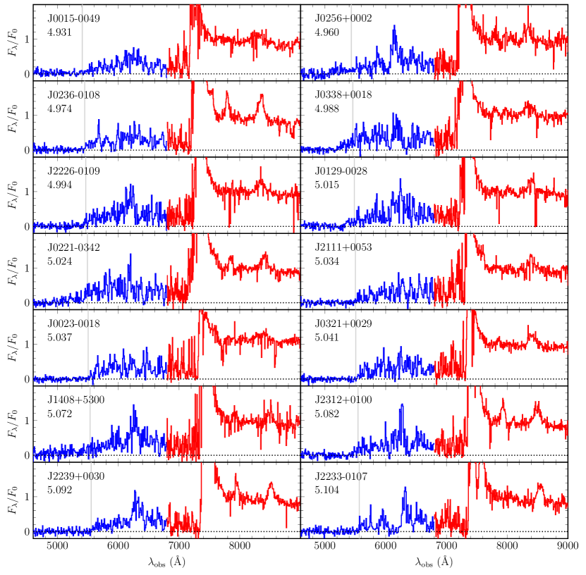
Figure 10: LRIS spectra used in this work. Panels are labeled with the QSO name and redshift. For each QSO we plot flux per unit wavelength normalized by the continuum flux measured over rest-frame 1270–1380 Å. The blue-side data taken with the 300/5000 grism are shown in blue. The red-side data taken with the 831/8200 grating are shown in red. Vertical lines mark the Lyman limit wavelength in the rest frame of the QSO.

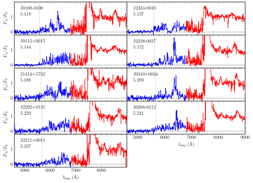
Figure 11: LRIS spectra used in this work (continued from Fig. 10)

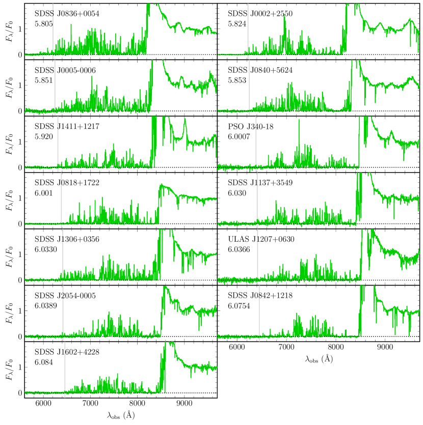
Figure 12: ESI and X-Shooter spectra used in this work. Panels are labeled with the QSO name and redshift. For each QSO we plot flux per unit wavelength normalized by the continuum flux measured over rest-frame 1270–1380 Å. The spectra have been median filtered using a 3-pixel sliding window. Vertical lines mark the Lyman limit wavelength in the rest frame of the QSO.

References

- Bañados et al. (2016) Bañados E., et al., 2016, ApJS, 227, 11
- Bañados et al. (2018) Bañados E., et al., 2018, Nature, 553, 473
- Becker & Bolton (2013) Becker G. D., Bolton J. S., 2013, MNRAS, 436, 1023
- Becker et al. (2011) Becker G. D., Bolton J. S., Haehnelt M. G., Sargent W. L. W., 2011, MNRAS, 410, 1096
- Becker et al. (2012) Becker G. D., Sargent W. L. W., Rauch M., Carswell R. F., 2012, ApJ, 744, 91
- Becker et al. (2013) Becker G. D., Hewett P. C., Worseck G., Prochaska J. X., 2013, MNRAS, 430, 2067
- Becker et al. (2015) Becker G. D., Bolton J. S., Madau P., Pettini M., Ryan-Weber E. V., Venemans B. P., 2015, MNRAS, 447, 3402
- Becker et al. (2018) Becker G. D., Davies F. B., Furlanetto S. R., Malkan M. A., Boera E., Douglass C., 2018, ApJ, 863, 92
- Becker et al. (2019) Becker G. D., et al., 2019, ApJ, 883, 163
- Boera et al. (2019) Boera E., Becker G. D., Bolton J. S., Nasir F., 2019, ApJ, 872, 101
- Bolton et al. (2012) Bolton J. S., Becker G. D., Raskutti S., Wyithe J. S. B., Haehnelt M. G., Sargent W. L. W., 2012, MNRAS, 419, 2880
- Bolton et al. (2017) Bolton J. S., Puchwein E., Haehnelt M. G., Kim T.-S., Meiksin A., Viel M., 2017, MNRAS, 464, 897
- Bosman et al. (2018) Bosman S. E. I., Fan X., Jiang L., Reed S., Matsuoka Y., Becker G., Haehnelt M., 2018, MNRAS, 479, 1055
- Cain et al. (2021) Cain C., D’Aloisio A., Gangolli N., Becker G. D., 2021, ApJ, 917, L37
- Calverley et al. (2011) Calverley A. P., Becker G. D., Haehnelt M. G., Bolton J. S., 2011, MNRAS, 412, 2543
- Carilli et al. (2010) Carilli C. L., et al., 2010, ApJ, 714, 834
- Chardin et al. (2018) Chardin J., Kulkarni G., Haehnelt M. G., 2018, MNRAS, 478, 1065
- Choudhury et al. (2020) Choudhury T. R., Paranjape A., Bosman S. E. I., 2020, arXiv:2003.08958
- Cooper et al. (2019) Cooper T. J., Simcoe R. A., Cooksey K. L., Bordoloi R., Miller D. R., Furesz G., Turner M. L., Bañados E., 2019, ApJ, 882, 77
- Cristiani et al. (2016) Cristiani S., Serrano L. M., Fontanot F., Vanzella E., Monaco P., 2016, MNRAS, 462, 2478
- D’Aloisio et al. (2018) D’Aloisio A., McQuinn M., Davies F. B., Furlanetto S. R., 2018, MNRAS, 473, 560
- D’Aloisio et al. (2020) D’Aloisio A., McQuinn M., Trac H., Cain C., Mesinger A., 2020, arXiv:2002.02467
- Davies & Furlanetto (2016) Davies F. B., Furlanetto S. R., 2016, MNRAS, 460, 1328
- Davies et al. (2018) Davies F. B., et al., 2018, ApJ, 864, 142
- Decarli et al. (2018) Decarli R., et al., 2018, ApJ, 854, 97
- Doughty & Finlator (2019) Doughty C., Finlator K., 2019, MNRAS, 489, 2755
- Eilers et al. (2017) Eilers A.-C., Davies F. B., Hennawi J. F., Prochaska J. X., Lukić Z., Mazzucchelli C., 2017, ApJ, 840, 24
- Eilers et al. (2018) Eilers A.-C., Davies F. B., Hennawi J. F., 2018, ApJ, 864, 53
- Fan et al. (2006) Fan X., et al., 2006, AJ, 132, 117
- Farina et al. (2019) Farina E. P., et al., 2019, ApJ, 887, 196
- Faucher-Giguère et al. (2008) Faucher-Giguère C.-A., Lidz A., Hernquist L., Zaldarriaga M., 2008, ApJ, 688, 85
- Fumagalli et al. (2013) Fumagalli M., O’Meara J. M., Prochaska J. X., Worseck G., 2013, ApJ, 775, 78
- Furlanetto & Oh (2005) Furlanetto S. R., Oh S. P., 2005, MNRAS, 363, 1031
- Gaikwad et al. (2020) Gaikwad P., et al., 2020, MNRAS, 494, 5091
- Greig et al. (2017) Greig B., Mesinger A., Haiman Z., Simcoe R. A., 2017, MNRAS, 466, 4239
- Greig et al. (2019) Greig B., Mesinger A., Bañados E., 2019, MNRAS, 484, 5094
- Haardt & Madau (1996) Haardt F., Madau P., 1996, ApJ, 461, 20
- Haardt & Madau (2012) Haardt F., Madau P., 2012, ApJ, 746, 125
- Horne (1986) Horne K., 1986, PASP, 98, 609
- Jung et al. (2020) Jung I., et al., 2020, ApJ, 904, 144
- Kashino et al. (2020) Kashino D., Lilly S. J., Shibuya T., Ouchi M., Kashikawa N., 2020, ApJ, 888, 6
- Keating et al. (2020a) Keating L. C., Weinberger L. H., Kulkarni G., Haehnelt M. G., Chardin J., Aubert D., 2020a, MNRAS, 491, 1736
- Keating et al. (2020b) Keating L. C., Kulkarni G., Haehnelt M. G., Chardin J., Aubert D., 2020b, MNRAS, 497, 906
- Kelson (2003) Kelson D. D., 2003, PASP, 115, 688
- Kuhlen & Faucher-Giguère (2012) Kuhlen M., Faucher-Giguère C.-A., 2012, MNRAS, 423, 862
- Kulkarni et al. (2019) Kulkarni G., Keating L. C., Haehnelt M. G., Bosman S. E. I., Puchwein E., Chardin J., Aubert D., 2019, MNRAS, 485, L24
- Lopez et al. (2016) Lopez S., et al., 2016, A&A, 594, A91
- Lusso et al. (2015) Lusso E., Worseck G., Hennawi J. F., Prochaska J. X., Vignali C., Stern J., O’Meara J. M., 2015, MNRAS, 449, 4204
- Lusso et al. (2018) Lusso E., Fumagalli M., Rafelski M., Neeleman M., Prochaska J. X., Hennawi J. F., O’Meara J. M., Theuns T., 2018, ApJ, 860, 41
- McGreer et al. (2013) McGreer I. D., et al., 2013, ApJ, 768, 105
- McGreer et al. (2018) McGreer I. D., Fan X., Jiang L., Cai Z., 2018, AJ, 155, 131
- McQuinn et al. (2011) McQuinn M., Oh S. P., Faucher-Giguère C.-A., 2011, ApJ, 743, 82
- Meiksin & Madau (1993) Meiksin A., Madau P., 1993, ApJ, 412, 34
- Miralda-Escude & Ostriker (1990) Miralda-Escude J., Ostriker J. P., 1990, ApJ, 350, 1
- Miralda-Escudé et al. (2000) Miralda-Escudé J., Haehnelt M., Rees M. J., 2000, ApJ, 530, 1
- Morales et al. (2021) Morales A., Mason C., Bruton S., Gronke M., Haardt F., Scarlata C., 2021, arXiv:2101.01205, 2101, arXiv:2101.01205
- Mortlock et al. (2011) Mortlock D. J., et al., 2011, Nature, 474, 616
- Nasir & D’Aloisio (2020) Nasir F., D’Aloisio A., 2020, MNRAS, 494, 3080
- O’Meara et al. (2013) O’Meara J. M., Prochaska J. X., Worseck G., Chen H.-W., Madau P., 2013, ApJ, 765, 137
- Oke et al. (1995) Oke J. B., et al., 1995, PASP, 107, 375
- Park et al. (2016) Park H., Shapiro P. R., Choi J.-h., Yoshida N., Hirano S., Ahn K., 2016, ApJ, 831, 86
- Planck Collaboration et al. (2020) Planck Collaboration et al., 2020, A&A, 641, A6
- Prochaska et al. (2009) Prochaska J. X., Worseck G., O’Meara J. M., 2009, ApJl, 705, L113
- Prochaska et al. (2014) Prochaska J. X., Madau P., O’Meara J. M., Fumagalli M., 2014, MNRAS, 438, 476
- Puchwein & Springel (2013) Puchwein E., Springel V., 2013, MNRAS, 428, 2966
- Qin et al. (2021) Qin Y., Mesinger A., Bosman S. E. I., Viel M., 2021, arXiv:2101.09033
- Rahmati & Schaye (2018) Rahmati A., Schaye J., 2018, MNRAS, 478, 5123
- Rahmati et al. (2013) Rahmati A., Pawlik A. H., Raičevic̀ M., Schaye J., 2013, MNRAS, 430, 2427
- Romano et al. (2019) Romano M., Grazian A., Giallongo E., Cristiani S., Fontanot F., Boutsia K., Fiore F., Menci N., 2019, A&A, 632, A45
- Rudie et al. (2013) Rudie G. C., Steidel C. C., Shapley A. E., Pettini M., 2013, ApJ, 769, 146
- Schirber & Bullock (2003) Schirber M., Bullock J. S., 2003, ApJ, 584, 110
- Scott et al. (2004) Scott J. E., Kriss G. A., Brotherton M., Green R. F., Hutchings J., Shull J. M., Zheng W., 2004, ApJ, 615, 135
- Shull et al. (2012) Shull J. M., Stevans M., Danforth C. W., 2012, ApJ, 752, 162
- Songaila & Cowie (2010) Songaila A., Cowie L. L., 2010, ApJ, 721, 1448
- Stevans et al. (2014) Stevans M. L., Shull J. M., Danforth C. W., Tilton E. M., 2014, ApJ, 794, 75
- Telfer et al. (2002) Telfer R. C., Zheng W., Kriss G. A., Davidsen A. F., 2002, ApJ, 565, 773
- Trac & Pen (2004) Trac H., Pen U.-L., 2004, New Astronomy, 9, 443
- Vanden Berk et al. (2001) Vanden Berk D. E., et al., 2001, AJ, 122, 549
- Venemans et al. (2020) Venemans B., et al., 2020, arXiv:2010.14874, 2010
- Walther et al. (2019) Walther M., Oñorbe J., Hennawi J. F., Lukić Z., 2019, ApJ, 872, 13
- Wang et al. (2020) Wang F., et al., 2020, ApJ, 896, 23
- Worseck et al. (2014) Worseck G., et al., 2014, MNRAS, 445, 1745
- Wyithe et al. (2008) Wyithe J. S. B., Bolton J. S., Haehnelt M. G., 2008, MNRAS, 383, 691
- Yang et al. (2020) Yang J., et al., 2020, ApJ, 904, 26