Gap-tunable of Tunneling Time in Graphene Magnetic Barrier

Youssef Fattasse^a, Miloud Mekkaoui^a, Ahmed Jellal^a,b and Abdelhadi Bahaoui^a

^aLaboratory of Theoretical Physics, Faculty of Sciences, Chouaïb Doukkali University,

PO Box 20, 24000 El Jadida, Morocco

^bCanadian Quantum Research Center, 204-3002 32 Ave Vernon,
BC V1T 2L7, Canada

We study the tunneling time of Dirac fermions in graphene magnetic barrier through an electrostatic potential and a mass term. This latter generates an energy gap in the spectrum and therefore affects the proprieties of tunneling of the system. For clarification, we first start by deriving the eigenspinors solutions of Dirac equation and second connect them to the incident, reflected and transmitted beam waves. This connection allows us to obtain the corresponding phases shifts and consequently compute the group delay time in transmission and reflection. Our numerical results show that the group delay time depends strongly on the energy gap in the tunneling process through single barrier. Moreover, we find that the group approaches unity at some critical value of the energy gap and becomes independent to the strengths of involved physical parameters.

PACS numbers: 81.05.ue; 73.63.-b; 73.23.-b; 73.22.Pr

Keywords: Graphene magnetic barrier, static potential, mass term, transmission, group delay time.

1 Introduction

In graphene sheets, the particles and density of the carriers can be controlled by tuning a gate bias voltage [1, 2, 3]. In a gapless graphene electrical conduction cannot be switched off by using the control voltages [4] that is essential for the operation of conventional transistors. This situation can be solved by generating an energy gap in the electronic spectrum of the carriers in graphene. Such gap is a measure of the threshold voltage and the on-off ratio of the field effect transistors [5, 6]. Experimentally, there are different techniques to open a gap in a graphene band structure [7] and its maximum value could be 260 meV because of the sublattice symmetry breaking [8]. We emphasis that its measurement varies from an experiment to another. For instance, an energy gap can be measured under the control of the structure of the interface between graphene and ruthenium [9] or by considering graphene grown epitaxially on a SiC substrate [8]. From theoretical point of view, alternative strategies have been proposed to generate an energy gap in systems based on graphene. There is a vast literature, but here we mention two developed strategies. Indeed, a graphene sheet on top of a lattice-matched hexagonal boron nitride (h-BN) substrate leading to a gap of 53 meV [9]. Also a graphene subject to the potential from an external superlattice can develop a gap provided the superlattice potential has a broken inversion symmetry [10, 11].

A basic quantum property is the tunnel effect that occurs when a particle passes through a potential barrier. Actually, it is known that under the increase of width and height of a barrier, the chance of a non-relativistic particle breaching it decreases exponentially. In contrast to the relativistic theory, which predicted that no matter how tall or wide the barrier is, a relativistic particle would tunnel through it with certainty. Such effect is called Klein tunneling that has been experimentally realized in graphene [12, 13, 14, 15]. On the other hand, the nanostructures based on graphene-magnetic barriers have recently been the subject of several investigations focusing on the tunneling time by treating time as a parameter rather than an observable in quantum mechanics [16, 17, 18, 19]. As a result, there is no straightforward way to quantify tunneling time. There are at least three different notions of traversing time in the literature for particles with a given energy [20]. To obtain the group delay time (called also phase time [21]), one first studies the evolution of the wave packets through the barrier, which requires the phase sensitivity of the tunneling amplitude to the incident energy of particles. In electron transport [22, 23, 24] and photon tunneling [25, 26], the group delay time has been described as one of the most important and interesting quantities. For instance, the group delay statistics are linked to dynamic admittance as well as other material microstructure properties [22] and to density of states [23, 24].

We investigate the group delay time for graphene magnetic field in the presence of a barrier potential and mass term. As a result we solve the Dirac equation in three regions to determine the solutions of the energy spectrum in terms of the energy gap $\Delta$. After matching the wave functions at interfaces and using the density current, we calculate the transmission and reflection probabilities. By mapping the incident, reflected and transmitted beam waves as functions of the eigenspinors we compute the group delay time. To give a better understanding of our results, we numerically investigate the basic features of the group and show that it can be controlled by tuning on $\Delta$. Moreover, we will discuss how the system parameters can affect the tunneling time in gapped graphene. In fact, we will study the main characteristics of this quantity in terms of the physical parameter of our system.

This paper is organized as follows. In section 2, we formulate our theoretical problem by writing the corresponding Hamiltonian and determine the eigenspinors and eigenvalues. In section 3, we use the boundary conditions together with current density to compute transmission and reflection probabilities that allow to derive the group delay time. We numerically discuss our results by giving different illustrations under suitable choices of the physical parameters, in section 4. Finally, we close our work by summarizing the main obtained results.

2 Theoretical model

We consider a system made of graphene having three regions labeled by $j={1},{2},{3}$ such that the medium region is subjected to a magnetic barrier together with a square potential and a mass term as geometrically represented in Figure 1. Note that, the mass term can be owing to the sublattice symmetry breaking or can be seen as the energy gap $\Delta=\Delta_{so}$ originating from the spin-orbit interaction. Near Dirac point ${\bm{K}}$, our system can be described by the Hamiltonian

$$H_{j}=v_{F}{\bm{\sigma}}\cdot\left({\bm{p}}+e{\bm{A}}\right)+V_{j}(x)\mathbb{I}_{2}+\Delta\Theta(Lx-x^{2})\sigma_{z}$$ (1)

where $v_{F}$ is the Fermi velocity, ${\bm{\sigma}}=(\sigma_{x},\sigma_{y})$ are the Pauli matrices and ${\mathbb{I}}_{2}$ is the $2\times 2$ unit matrix, $\Theta$ is the step function. We use a static square potential barrier of the form

$$V_{j}(x)=\left\{\begin{array}[]{ll}V_{0},&\qquad\hbox{$0\leq x\leq L$}\\ 0,&\qquad\hbox{otherwise}.\\ \end{array}\right.$$ (2)

Regarding a magnetic barrier, the relevant physics is described by a magnetic field translationally invariant along the $y$-direction $B(x,y)=B(x)$. It is associated to the vector potential in Landau gauge ${\bm{A}}=(0,A_{y}(x))^{T}$ since $\partial_{x}A_{y}(x)=B(x)$ and consequently the transverse momentum $p_{y}$ is a conserved quantity. In our study we consider $\textbf{B}=B\textbf{e}_{z}$ along $z$-direction within the strip $0\leq x\leq L$ but $B=0$ elsewhere, namely $B(x,y)=B\Theta(Lx-x^{2})$, with $B$ is a constant. Due to the continuity, we have the potential

$$\qquad A_{y}(x)=\left\{\begin{array}[]{ll}0,&\qquad\hbox{$x<0$}\\ Bx,&\qquad\hbox{$0\leq x\leq L$}\\ BL,&\qquad\hbox{$x>L$}.\\ \end{array}\right.$$ (3)

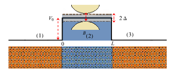
(a)

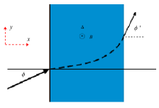
(b)

Figure 1: (color online) (a): Schematic of the potential profile in graphene magnetic barrier with mass term, forming three regions denoted by $j=1,2,3$. (b): Trajectory for an electron of our system having the incident angle $\phi$ and the transmitted angle $\phi^{\prime}$.

The solutions of energy spectrum associated to (1) can be obtained by solving Dirac equation for the spinor $\Psi_{j}(x,y)=e^{ik_{y}y}(\varphi^{+}_{j}(x),\varphi^{-}_{j}(x))^{T}$

$$\left[{\bm{\sigma}}\cdot\frac{1}{\hbar}\left({\bm{p}}+e{\bm{A}}\right)+\tilde{V}_{j}(x)\mathbb{I}_{2}+\tilde{\Delta}\Theta(Lx-x^{2})\sigma_{z}\right]\Psi_{j}(x,y)=\epsilon\Psi_{j}(x,y)$$ (4)

and we have set the quantities $\epsilon=E/\hbar\upsilon_{F}$, $\tilde{V}=\frac{V}{\hbar v_{F}}$ and $\tilde{\Delta}=\frac{\Delta}{\hbar v_{F}}$. Consequently, in region $1$ $(x<0)$, the solution is obtained as sum of incident $\Psi_{\sf in}(x,y)$ and reflected $\Psi_{\sf re}(x,y)$ waves that is

$$\Psi_{1}(x,y)=\frac{1}{\sqrt{2}}\begin{pmatrix}1\\ e^{i\phi}\end{pmatrix}e^{i(k_{x}x+k_{y}y)}+\frac{r}{\sqrt{2}}\begin{pmatrix}1\\ -e^{-i\phi}\end{pmatrix}e^{i(-k_{x}x+k_{y}y)}$$ (5)

where $r$ is the reflection amplitude and the wave vector component is defined in terms of the incident energy $\epsilon$ as

$$k_{x}=s\sqrt{\epsilon^{2}-k^{2}_{y}}.$$ (6)

It is convenient for our task to express the wave vector components $k_{x}$ and $k_{y}$ in terms of the incident angle $\phi$. Thus, we can write

$$k_{x}=\epsilon\cos\phi,\qquad k_{y}=\epsilon\sin\phi$$ (7)

As far as region $3$ $(x>L)$ is concerned, we solve (4) to end up with the eigenspinor $\psi_{3}(x,y)$ for transmitted electron

$$\Psi_{3}(x,y)=\frac{t}{\sqrt{2}}\begin{pmatrix}1\\ e^{i\phi^{\prime}}\end{pmatrix}e^{ik^{\prime}_{x}x+k_{y}y}$$ (8)

where $t$ is the transmission amplitude and we have

$$k^{\prime}_{x}=\sqrt{\epsilon^{2}-(k_{y}+\beta L)^{2}}$$ (9)

such that $\beta=\frac{eB}{\hbar}$ has the inverse of length. The transmitted angle is related to the wave vector components via

$$k^{\prime}_{x}=\epsilon\cos\phi^{\prime},\qquad k_{y}=\epsilon\sin\phi^{\prime}-\beta L$$ (10)

and consequently we establish the relation

$$\sin\phi^{\prime}=\sin\phi+\frac{\beta L}{\epsilon}.$$ (11)

Regarding region 2 ($0\leq x\leq L$), let us first write the corresponding Hamiltonian in terms of the annihilation $a^{-}$ and creation $a^{+}$ operators

$$H_{2}=\hbar v_{F}\left(\begin{array}[]{cc}V^{+}&-i\sqrt{2\beta}a^{-}\\ i\sqrt{2\beta}a^{+}&V^{-}\\ \end{array}\right)$$ (12)

such that $V^{\pm}=\tilde{V}\pm\tilde{\Delta}$ and we have

$$a^{\pm}=\frac{1}{\sqrt{2\beta}}\left(\mp\partial_{x}+k_{y}+x\beta\right)$$ (13)

which satisfy the commutation relation $[a,a^{\dagger}]=\mathbb{I}$. As usual, we solve the eigenvalue equation for $\psi_{2}(x,y)=e^{ip_{y}y}(\varphi_{2}^{+}(x),\varphi_{2}^{-}(x))^{T}$

$$H_{2}\left(\begin{array}[]{c}\varphi_{2}^{+}\\ \varphi_{2}^{-}\\ \end{array}\right)=\hbar v_{F}\epsilon\left(\begin{array}[]{c}\varphi_{2}^{+}\\ \varphi_{2}^{-}\\ \end{array}\right)$$ (14)

to obtain two coupled equations

$$V^{+}\varphi_{2}^{+}-i\sqrt{2\beta}a^{-}\varphi_{2}^{-}=\epsilon\varphi_{2}^{+}$$ (15)

$$i\sqrt{2\beta}a^{+}\varphi_{2}^{+}+V^{-}\varphi_{2}^{-}=\epsilon\varphi_{2}^{-}.$$ (16)

Injecting (16) into (15) we end up with a differential equation of second order for $\varphi_{2}^{+}$

$$\left(\epsilon-V^{+}\right)\left(\epsilon-V^{-}\right)\varphi_{2}^{+}=2\beta a^{-}a^{+}\varphi_{2}^{+}.$$ (17)

This is in fact an equation of the harmonic oscillator and therefore we identify $\varphi_{2}^{+}$ with its eigenstates $|n-1\rangle$ associated to the eigenvalues

$$\tilde{\varepsilon}=\sqrt{2\beta n+\tilde{\Delta}^{2}}$$ (18)

where we have set $\tilde{\varepsilon}=s^{\prime}\left(\epsilon-\tilde{V}\right)$, $s^{\prime}=\mbox{sign}\left(\epsilon-\tilde{V}\right)$ correspond to positive and negative energy solutions. From (16), we derive the second spinor component

$$\varphi^{-}_{2}=s^{\prime}i\sqrt{\frac{\tilde{\varepsilon}-s^{\prime}\tilde{\Delta}}{\tilde{\varepsilon}+s^{\prime}\tilde{\Delta}}}\mid n\rangle.$$ (19)

Combing all components we can map the eigenspinors in terms of the parabolic cylinder functions $D_{n}(x)=2^{-\frac{n}{2}}e^{-\frac{x^{2}}{4}}H_{n}\left(\frac{x}{\sqrt{2}}\right)$ as

$$\Psi_{\sf 2}(x,y)=e^{ik_{y}y}\sum_{\pm}c^{\pm}\begin{pmatrix}\sqrt{\frac{\tilde{\varepsilon}+s^{\prime}\tilde{\Delta}}{\tilde{\varepsilon}}}D_{\left(\tilde{\varepsilon}^{2}-\tilde{\Delta}^{2}\right)/2\beta-1}\left(\pm\sqrt{\frac{2}{\beta}}\left(\beta x+k_{y}\right)\right)\\ \frac{\pm i\sqrt{2\beta}}{\sqrt{\tilde{\varepsilon}\left(\tilde{\varepsilon}+s^{\prime}\tilde{\Delta}\right)}}D_{\left(\tilde{\varepsilon}^{2}-\tilde{\Delta}^{2}\right)/2\beta}\left(\pm\sqrt{\frac{2}{\beta}}\left(\beta x+k_{y}\right)\right)\\ \end{pmatrix}$$ (20)

with the Hermite polynomials $H_{n}(x)$. Note that, the transmission $t$ and reflection $r$ coefficients will be determined by using the boundary conditions at interfaces.

3 Group delay time

We study the group delay time in transmission and reflection beams around some transverse wave vector $k_{y}$ and incident angle $\phi\in[0,\frac{\pi}{2}]$ fulfilling the relation (11). This is because the wave incident from the right- and left-hand sides of the surface normal will behave differently [27]. Then, we characterize our waves by introducing a critical angle $\phi_{c}$ defined by

$$\phi_{c}=\arcsin\left[1-\frac{L\beta}{\epsilon}\right]$$ (21)

which corresponds to take $\phi^{\prime}=\frac{\pi}{2}$ in (11). Consequently, an immediate conclusion takes place such that we have oscillating guided modes when $\phi<\phi_{c}$ and decaying or evanescent wave modes in the opposite case. As a matter of simplicity, we will be interested in studying the case $\phi<\phi_{c}$ in the forthcoming analysis.

Based on different considerations, we study the interesting properties of our system in terms of the corresponding transmission and reflection probabilities. To start we use the continuity of eigenspinors at the interfaces $x=0$ and $x=L$ to write the boundary conditions

$$\Psi_{1}(0,y)=\Psi_{2}(0,y),\qquad\Psi_{2}(L,y)=\Psi_{3}(L,y)$$ (22)

which give rise to a set of equations. Then after a lengthy but straightforward algebra, we show that the transmission and reflection coefficients take the forms

$$t=\frac{2\xi_{1}\xi_{2}}{\chi}(u_{1L}v_{2L}+u_{2L}v_{1L})\cos{\phi}$$ (23)

$$r=\frac{\Lambda}{\chi}$$ (24)

where we have defined the quantities

$$\chi=\left(\xi_{2}u_{20}-\xi_{1}u_{10}e^{-i\phi}\right)\left(\xi_{1}v_{1L}e^{i\phi^{\prime}}-\xi_{2}v_{2L}\right)+\left(\xi_{1}u_{1L}e^{i\phi^{\prime}}+\xi_{2}u_{2L}\right)\left(\xi_{2}v_{20}+\xi_{1}v_{10}e^{-i\phi}\right)$$ (25)

$$\Lambda=\left(-\xi_{2}u_{20}-\xi_{1}u_{10}e^{i\phi}\right)\left(\xi_{1}v_{1L}e^{i\phi^{\prime}}-\xi_{2}v_{2L}\right)+\left(\xi_{1}u_{1L}e^{i\phi^{\prime}}+\xi_{2}u_{2L}\right)\left(-\xi_{2}v_{20}+\xi_{1}v_{10}e^{i\phi}\right)$$ (26)

and the following shorthand notation

$$u_{1x}=D_{\left(\tilde{\varepsilon}^{2}-\tilde{\Delta}^{2}\right)/2\beta-1}\left(\sqrt{\frac{2}{\beta}}\left(\beta x+k_{y}\right)\right),\qquad u_{2x}=D_{\left(\tilde{\varepsilon}^{2}-\tilde{\Delta}^{2}\right)/2\beta}\left(-\sqrt{\frac{2}{\beta}}\left(\beta x+k_{y}\right)\right)$$ (27)

$$v_{1x}=D_{\left(\tilde{\varepsilon}^{2}-\tilde{\Delta}^{2}\right)/2\beta-1}\left(\sqrt{\frac{2}{\beta}}\left(\beta x+k_{y}\right)\right),\qquad v_{2x}=D_{\left(\tilde{\varepsilon}^{2}-\tilde{\Delta}^{2}\right)/2\beta}\left(-\sqrt{\frac{2}{\beta}}\left(\beta x+k_{y}\right)\right)$$ (28)

$$\xi_{1}=\sqrt{\frac{\tilde{\varepsilon}+s^{\prime}\tilde{\Delta}}{\tilde{\varepsilon}}},\qquad\xi_{2}=\frac{i\sqrt{2\beta}}{\sqrt{\tilde{\varepsilon}\left(\tilde{\varepsilon}+s^{\prime}\tilde{\Delta}\right)}}.$$ (29)

It is easy to show the mapping

$$t=|t|e^{i\varphi_{t}},\qquad t=|r|e^{i\varphi_{r}}$$ (30)

in terms of the phase shifts $\varphi_{t}$ and $\varphi_{r}$. Both relations will play a crucial rule in computing the group delay time associated to our system.

To determine the transmission $T$ and reflection $R$ probabilities, we introduce the current density, which can be found to be

$$J=ev_{F}\psi^{+}\sigma_{x}\psi$$ (31)

which allows to obtain its incident $J_{\sf in}$, transmitted $J_{\sf tr}$ and reflected $J_{\sf re}$ components. Then, from the relations $T=\frac{|J_{\sf tr}|}{|J_{\sf in}|}$ and $R=\frac{|J_{\sf re}|}{|J_{\sf in}|}$ we get the results

$$T=\frac{k^{\prime}_{x}}{k_{x}}|t|^{2},\qquad R=|r|^{2}.$$ (32)

In the next, we show how the above tools can be used to study the group delay time in transmission and reflection. In the beginning, let us notice that a finite pulsed electron beam can be represented by a tempo-spatial wave packet as weighed superposition of plane wave spinors. As a results, we can express the incident, reflected and transmitted beam waves at $x=0$ as double Fourier integrals over $\omega$ and $k_{y}$ [29, 28]. They are

$$\Phi_{\sf in}(x,y,t)=\iint f(k_{y},\omega)\ \Psi_{\sf in}(x,y)\ e^{-i\omega t}\ dk_{y}d\omega$$ (33)

$$\Phi_{\sf re}(x,y,t)=\iint f(k_{y},\omega)\ \Psi_{\sf re}(x,y)\ e^{-i\omega t}\ dk_{y}d\omega$$ (34)

$$\Phi_{\sf tr}(x,y,t)=\iint f(k_{y},\omega)\ \Psi_{\sf tr}(x,y)\ e^{-i\omega t}\ dk_{y}d\omega$$ (35)

where the three spinors $\Psi_{\sf in},\Psi_{\sf re}$ and $\Psi_{\sf tr}$ are given in (5) and (8), respectively. The frequency of wave is $\omega=E/\hbar$ and the angular spectral distribution is assumed to be of Gaussian shape, i.e. $f(k_{y},\omega)=w_{y}e^{-w_{y}^{2}(k_{y}-\omega)^{2}}$ with the half beam width at waist $w_{y}$ [30]. From (34-35), we get the total phases for the reflected and transmitted waves functions at ($x=0$, $x=L$), which are

$$\phi_{r}=\varphi_{r}+k_{y}y-\omega t,\qquad\phi_{t}=\varphi_{t}+(k_{y}+\beta L)y-\omega t.$$ (36)

To determine the Goos-Hänchen (GH) shifts $S_{\gamma}$ and group delay time $\tau_{\gamma}$, one can use the stationary phase approximation [31, 32]. In this case $S_{\gamma}$ is given by

$$S_{\gamma}=-\frac{\partial\varphi_{\gamma}}{\partial k_{y}}$$ (37)

where $\gamma=t,r$ stands for transmission and reflection. As for $\tau_{\gamma}$ we use the two derivatives of phase shifts with respect to the incident angle $\phi$ and frequency $\omega$. Then from the conditions

$$\frac{\partial\varphi_{\gamma}}{\partial\phi}=0,\qquad\frac{\partial\varphi_{\gamma}}{\partial\omega}=0$$ (38)

we end up with a result

$$\tau_{\gamma}=\tau^{\varphi_{\gamma}}+\tau^{s_{\gamma}}$$ (39)

as sum of two parts

$$\tau^{\varphi_{\gamma}}=\frac{\partial\varphi_{\gamma}}{\partial\omega},\qquad\tau^{s_{\gamma}}=\left(\frac{\partial k_{y}}{\partial\omega}\right)S_{\gamma}$$ (40)

such that $\tau^{\varphi_{\gamma}}$ represents the time derivative of phase shifts, while $\tau^{s_{\gamma}}$ results from the contribution of the shift $S_{\gamma}$. Since the wave function is involving two-component spinor then $\tau_{\gamma}$ can be regarded as average of the group delay times of two components. Consequently, we have in phase shifts

$$\tau^{\varphi_{t}}=\hbar\frac{\partial\varphi_{t}}{\partial E}+\frac{\hbar}{2}\frac{\partial\phi^{\prime}}{\partial E},\qquad\tau^{\varphi_{r}}=\hbar\frac{\partial\varphi_{r}}{\partial E}$$ (41)

and in GH shifts

$$\tau^{s_{t}}=\frac{\sin\phi}{\upsilon_{F}}S_{t},\qquad\tau^{s_{r}}=\frac{\sin\phi}{\upsilon_{F}}S_{r}.$$ (42)

These results will be numerically investigated to emphasis the basic features of our system. It will help us to understand the effect of various potential parameters on the group delay time of a gap opening in graphene magnetic barrier scattered by a square potential.

4 Numerical results

To numerically study the transmission probability $T$ and group delay time $\tau_{\gamma}$ for our system, we first fix some requirements needed. Indeed, according to (9) we show that the magnetic field $B$ should fulfill the condition

$$\frac{\sqrt{|(E-V)^{2}-\Delta^{2}|}}{eL\upsilon_{F}}<B<\frac{E}{eL\upsilon_{F}}$$ (43)

in order to have a real wave vector $k^{\prime}_{x}$. Then beyond this, $k^{\prime}_{x}$ will be imaginary, which physically entails the evanescence of the wave function inside the barrier. In contrast, when the magnetic field satisfies (9), the evanescent wave function exists, but still propagating inside the transmission region. As a result, for our numerical analysis, we choose the parameters $\phi=0$, $V=80$ meV, $E=125$ meV, $\Delta=20$ meV, $L=75$ nm to get the magnetic interval 0.53 T $<B<$ 1.67 T. Additionally, in each configuration a set of appropriate values of physical parameters will be fixed depending on the plots. These will result in generating interesting information regarding our system and may shed some light on its possible technological application. In the next and for numerical reason we use dimensionless group delay time $\tau_{t}/\tau_{0}$ by introducing a time scale $\tau_{0}=L/v_{F}$. In fact this will help to understand and determine the particle velocities when cross the barrier either greater or less than that of Fermi.

Figure 2 shows the transmission probability $T$ and group delay time $\tau_{t}/\tau_{0}$ as a function of the energy gap $\Delta$ for three values of magnetic field $B=0.1$ T (red), $0.3$ T (blue), $0.4$ T (green) with barrier height $V_{0}=80$ meV and width $L=70$ nm. In panel 2a, we distinguish two energy zones such that in the first one $\Delta$ $<E-V_{0}$, there is full transmission (Klein tunneling) even with the increase of $\Delta$ because the wave vector inside the barrier is real corresponding to the transmission mode. Whereas in the second zone $\Delta$ $>E-V_{0}$, we notice that $T$ decays exponentially as long as $\Delta$ increases and later on it approaches to zero because the wave vector $k_{x}$ inside the barrier becomes imaginary giving rise to an evanescent mode. Additionally, according the values taken by $B$ we observe that $T$ decreases rapidly as $B$ increased. In panel 2b, we observe that for $\Delta$ $=0$ and $B=0.1$ T (red) the particles propagate through the barrier with the Fermi velocity $v_{F}$ ($\tau_{t}/\tau_{0}=1$) but by increasing $\Delta$ one sees that $\tau_{t}/\tau_{0}$ start to increase slowly to reach a maximum and after that it decreases rapidly toward a constant value, which becomes independent of $\Delta$. We notice that $B$ affects the behavior of $\tau_{t}/\tau_{0}$ because it decreases when $B$ increases.

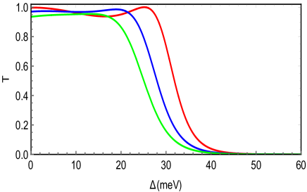
(a) $B$=0.1 T, 0.3 T, 0.4 T

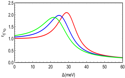
(b) $B$=0.1 T, 0.3 T, 0.4 T

Figure 2: (color online) Panel (a): The transmission $T$ and panel (b): group delay in transmission $\tau/\tau_{0}$ as a function of the energy gap $\Delta$ for three values of the magnetic field $B=0.1$ T (red), $0.3$ T (blue), $0.4$ T (green) with $\phi=0$, $E=120$ meV, $V=80$ meV, $L=70$ nm.

In Figure 3 we plot the group delay time $\tau_{t}$ as a function of the incident energy $E$ for various physics parameters. Indeed, panel 3a illustrates the case of three values of the incident angle $\phi=25$ (red), $30$ (blue), $35$ (green) for $V_{0}=80$ meV, $B=0.5$ T, $L=100$ nm and $\Delta=20$ meV. We observe that $\tau_{t}$ oscillates with the increase of $E$ and also its peak increases as long as $\phi$ increases, but when $E$ becomes larger than a critical value $E_{c}=40$ meV, $\tau_{t}$ approaches quickly zero. Panel 3b shows the influences of the barrier widths $L=65$ nm (red), $95$ nm (blue), $122$ nm (green) with $V_{0}=80$ meV, $B=0.4$ T, $\phi=30$ and $\Delta=10$ meV. When $E<E_{c}$, $\tau_{t}$ shows oscillatory behavior with different amplitudes and the number of oscillations increases with the increase of $L$. Another important remark is that when $L$ becomes large enough $\tau_{t}$ becomes independent of $E$. We notice that when $E$ is larger than $E_{c}$, $\tau_{t}$ goes to stabilize at zero whatever the value of $L$. In panel 3c we consider three values of magnetic field $B=0.4$ T (red), $0.5$ T (blue), $0.6$ T (green) for $V_{0}=80$ meV, $L=95$ nm, $\phi=30$ and $\Delta=10$ meV. It is clearly seen that $B$ affects the oscillatory behavior of $\tau_{t}$ because its peaks get decreased by increasing $B$ and their positions shifted clockwise as well. Panel 3d presents three values of the energy gap $\Delta=10$ meV (red), $20$ meV (blue), $\Delta=30$ meV (green), for $V_{0}=80$ meV, $L=100$ nm, $\phi=30$ and $B=0.5$ T. As for the case $E<E_{c}$, we observe that $\tau_{t}$ oscillates with different amplitudes. Now by increasing $\Delta$, we notice that there is an important increase of $\tau_{t}$ and their peaks also get affected in position and value.

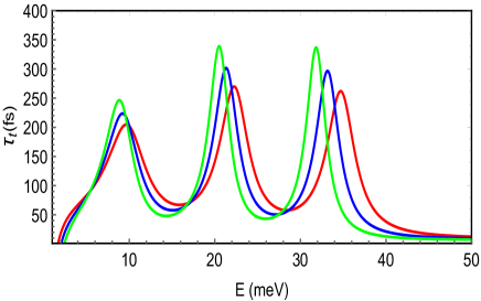
(a) $\phi=25,30,35$

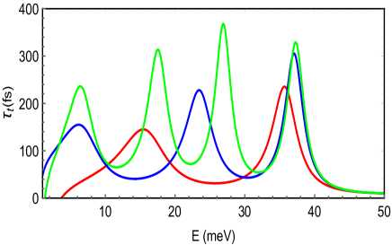
(b) $L=65\ \mbox{nm},85\ \mbox{nm},122\ \mbox{nm}$

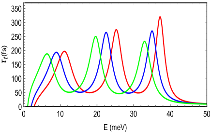
(c) $B=0.4\ \mbox{T},0.5\ \mbox{T},0.6\ \mbox{T}$

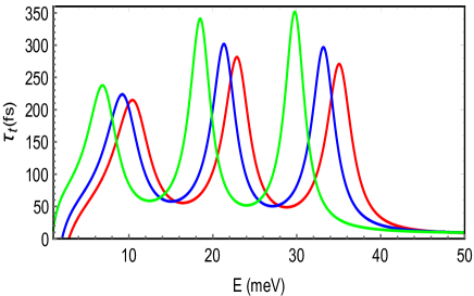
(d) $\Delta=10\ \mbox{meV},20\ \mbox{meV},30\ \mbox{meV}$

Figure 3: (color online) The group delay time in transmission $\tau_{t}$ as a function of the incident energy $E$ for the barrier height $V_{0}=80$ meV. Panel (a): $\phi$= 25 (red), 30 (blue), 35 (green) with $B=0.5$ T, $L=100$ nm, $\Delta=20$ meV. Panel (b): $L$=65 nm (red), 85 nm (blue), 122 nm (green) with $B=0.4$ T, $\Delta=10$ meV, $\phi=30$. Panel (c): $B$=0.4 T (red), 0.5 T (blue), 0.6 T (green) with $L=95$ nm, $\Delta=10$ meV, $\phi=30$. Panel (d): $\Delta$= 10 meV (red), 20 meV (blue), 30 meV (green) with $B=0.5$ T, $L=100$ nm, $\phi=30$.

Figure 4 presents the group delay time $\tau_{t}$ as function of the barrier height $V_{0}$ for $E=80$ meV and under suitable choices of physical parameters. Panel 4a present the effect of three values of the incident angle $\phi=25$ (red), $30$ (blue), $35$ (green) for $B=0.5$ T, $L=100$ nm and $\Delta=20$ meV. We observe that $\tau_{t}$ oscillates by decreasing when $V_{0}$ increases and goes to a constant value after some critical value of $V_{0}$. Also its peaks decrease as long as $\phi$ increases because for $V_{0}=0$, $\tau_{t}$ has maximal value for $\phi=25$ compared to $\phi=30$ and $\phi=35$. It is interesting to stress that for different values of $\phi$, $\tau_{t}$ does not oscillate in the same manner. Moreover, for $V_{0}\geq 40$ meV one sees that $\tau_{t}$ becomes not sensitive to any increase of $V_{0}$ and converges to a constant value. In panel 4b we take three values of the barrier width $L=80$ nm (red), $90$ nm (blue), $95$ nm (green) for $\phi=30$, $B=0.4$ T and $\Delta=20$ meV. It is clear that $\tau_{t}$ represents an oscillatory behavior and its peaks oscillate in the same manner but their values increase with $L$. Furthermore as for $V_{0}\geq 40$ meV, $\tau_{t}$ becomes independent of $L$ and shows saturation to a constant value. Panel 4c shows the effect of three values of magnetic field $B=0.4$ T (red), $0.5$ T (blue), $0.6$ T (green) for $L=100$ nm, $\phi=30$ and $\Delta=20$ meV. We notice that $\tau_{t}$ oscillates with the increase of $V_{0}$ and also is modulated by the presence of $B$ because when $B$ increases $\tau_{t}$ decreases. We observe that when $V_{0}$ exceeds $25$ meV, $\tau_{t}$ is not influenced and remains constant whatever the value taken by $V_{0}$ and $B$. In panel 4d we consider the influence of three values of energy gap $\Delta=10$ meV (red), $20$ meV (blue), $30$ meV (green) for $\phi=30$, $B=0.5$ T, $L=100$ nm. It shows that the peak of $\tau_{t}$ increases by increasing $\Delta$ and $V_{0}$. One can see that when $V_{0}\geq 30$ the group delay time $\tau_{t}$ saturates to a constant value. We conclude that $\Delta$ moderates the variation of $\tau_{t}$ toward a tunable way.

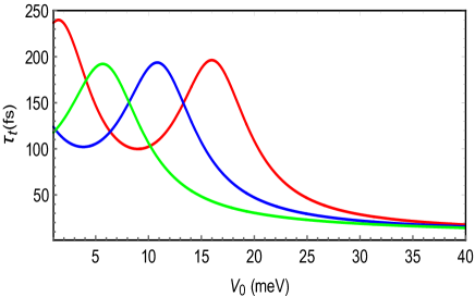
(a) $\phi=25$, $30$, $35$

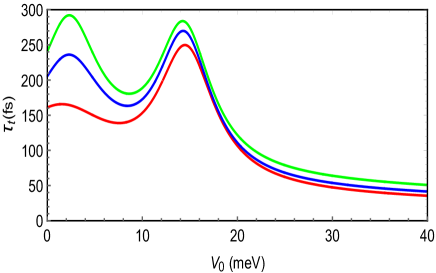
(b) $L=80$ nm, 90 nm, 95 nm

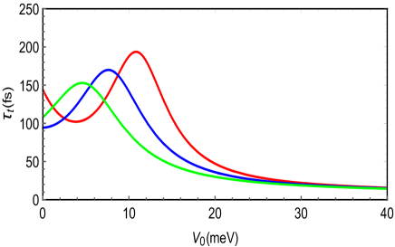
(c) $B=0.4$ T, $0.5$ T, $0.6$ T

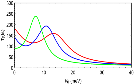
(d) $\Delta=10$ meV, $20$ meV, $30$ meV

Figure 4: (color online) The group delay time in transmission as a function of barrier height $V_{0}$ for the incident energy $E=80$ meV. Panel (a): $\phi$= 25 (red), 30 (blue), 35 (green), $B=0.5$ T, $L=100$ nm, $\Delta=20$ meV. Panel (b): $L$=(80 nm, $90$ nm, $95$ nm), $\phi=30$, $B=0.4$ T, $\Delta=20$ meV. Panel (c): $B=0.4$ T (red), $0.5$ T (blue), $0.6$ T (green), $L=100$ nm, $\Delta=20$. Panel (d): $\Delta$=10 meV (red), $20$ meV (blue), $30$ meV (green), $\phi=30$, $B=0.5$ T, $L=100$ nm.

Figure 5 presents the group delay time in reflection $\tau_{r}$ as a function of the incident energy $E$ and barrier height $V_{0}$ with the configuration $L=100$ nm, $\phi=30$, $\Delta=20$. We recall that $\tau_{r}$ contains two parts such that the phase group delay $\tau^{\varphi_{r}}$ and that resulted from GH shifts $\tau^{s_{r}}$. In panel 5a we choose $V_{0}=80$ meV and observe that $\tau^{s_{r}}$ (red) and $\tau^{\varphi_{r}}$ (blue) are oscillating differently because $\tau^{s_{r}}$ shows positive behavior and $\tau^{\varphi_{r}}$ negative one. The resulting $\tau_{r}$ (green) oscillates from negative for small range of $E$ to positive for a large range. Now in panel 5b we choose $E=80$ meV and observe that all contribution to $\tau^{\varphi_{r}}$ are oscillating positively by showing only one peak and decrease quickly to zero as long as $V_{0}$ increase.

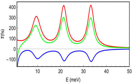
(a)

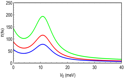
(b)

Figure 5: (color online) The group delay time $\tau_{r}=\tau^{s_{r}}+\tau^{\varphi_{r}}$ in reflection as a function of the incident energy $E$ and the potential barrier $V_{0}$. Panel (a): $V_{0}=80$ meV and panel (b): $E=80$ meV for $\phi=30$, $B=0.5$ T, $L=100$ nm, $\Delta=20$ meV, with $\tau_{r}$ (green), $\tau^{s_{r}}$ (blue), $\tau^{\varphi_{r}}$ (red).

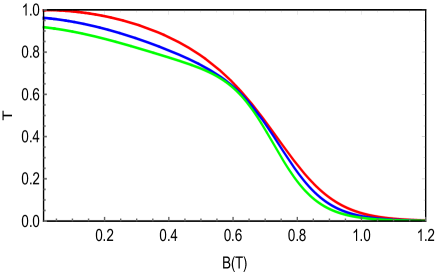
(a) $\Delta=0$ meV, 9 meV, 13 meV

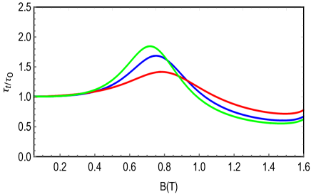
(b) $\Delta=0$ meV, 9 meV, 13 meV

Figure 6: (color online) Panel (a): transmission $T$ and panel (b): group delay time in transmission $\tau/\tau_{0}$ as a function of the magnetic field $B$ for three values of energy gap $\Delta$=0 meV (red), 9 meV (blue), 13 meV (green) with $\phi=0$, $E=125$ meV, $V=80$ meV, $L$=75 nm.

In Figure 6 we plot the transmission $T$ and group delay time $\tau_{t}/\tau_{0}$ as a function of the magnetic field $B$ for three values of energy gap $\Delta=0$ meV (red), $9$ meV (blue), $13$ meV (green) with $\phi=0$, $E=125$ meV, $V=80$ meV and $L=75$ nm. For null $\Delta$ (red) panel 6a tells us that $T$ decays exponentially toward zero as long as $B$ increases. Now for no-null $\Delta$ (blue, green) we observe that $T$ shows the same behavior as before except that $\Delta$ acts by diminishing the amplitude of $T$, which means that $T$ decreases rapidly with the increase of $\Delta$. In panel 6b, we observe that for the barrier static $B$ $=0$ the particles propagate through the barrier with the Fermi velocity $v_{F}$ ($\tau_{t}/\tau_{0}=1$), we notice that for the magnetic field less than $0.4$ T, the particles propagate through the barrier with the Fermi velocity $v_{F}$, but when $B$ is in the range [$0.4$ T, $1$ T], $\tau_{t}/\tau_{0}$ is subluminal, which can be changed from subluminal to superluminal. With the increase of $B$, we observe that $\tau_{t}/\tau_{0}$ decreases and becomes less than $L/v_{F}$, i.e. $\tau_{t}<\tau_{0}$. Note that for different values of $\Delta$, the peak of $\tau_{t}/\tau_{0}$ increases as long as $B$ increases. As we increase the energy gap $\Delta$ we observe that the oscillations set in much earlier.

5 Conclusion

We have studied the tunneling time in graphene magnetic barrier scattered by a scalar potential and subject to a mass term. Taking into account the advantage of an opening gap in the energy spectrum we have analyzed the corresponding group delay time. To do that we have first solved Dirac equation to obtain the eigenspinors and used the boundary conditions at interfaces together with current density to determine the transmission and reflection probabilities. After establishing a link between our eigenspinors and beam waves, we have showed that the group delay time has two contributions resulted from phase shifts and that of Goos-Hänchen (GH). More precisely, we have derived analytic expressions for the group delay time by taking into account the lateral displacement resulting from the angular spread of the incident electron wave packet. In fact, a total group $\tau_{t}$ involving two parts such as the phase group delay $\tau^{\varphi_{t}}$ and the group delay contributing from the lateral GH shifts $\tau^{s_{t}}$ is obtained.

Subsequently, we have numerically analyzed the group delay time by considering various choice of the physical parameters. Indeed, to start we have fixed the magnetic interval that allowed us to generate interesting results. Particularly in the propagating case, we have showed that the group delay time is greatly enhanced by transmission resonances thanks to the presence of energy gap. Additionally, at different occasion we have noticed that at some large values of the involved physical parameters the group delay time becomes insensible of the increase of them and converges toward constant values. As a result, the group delay time in transmission $\tau_{t}/\tau_{0}$ can be controlled by tuning on $\Delta$ in orienting experiments to engineer new systems for potential applications.

References

- [1] K. S. Novoselov, A. K. Geim, S. V. Morozov, D. Jiang, M. I. Katsnelson, I. V. Grigorieva, S. V. Dubonos, and A. A. Firsov, Nature 438, 197 (2005).
- [2] Y. B. Zhang, Y. W. Tan, H. L. Störmer, and P. Kim, Nature 438, 201 (2005).
- [3] J. Nilsson, A. H. Castro Neto, F. Guinea, and N. M. R. Peres, Phys. Rev. B 76, 165416 (2007).
- [4] M. I. Katsnelson, K. S. Novoselov, and A. K. Geim, Nature Phys. 2, 620 (2006).
- [5] Y. Lin, K. A. Jenkins, A. Valdes-Garcia, J. P. Small, D. B. Farmer, and P. Avouris, Nano Lett. 9, 422 (2009).
- [6] J. Kedzierski, P. Hsu, P. Healey, P. W. Wyatt, C. L. Keast, M. Sprinkle, C. Berger, and W. A. de Heer, IEEE Trans. Electron Devices 55, 2078 (2008).
- [7] D. S. L. Abergel, V. Apalkov, J. Berashevich, K. Ziegler and T. Chakraborty, Adv. Phys. 59, 261 (2010).
- [8] C. Enderlein, Y. S. Kim, A. Bostwick, E. Rotenberg and K. Horn, New. J. Phys. 12, 033014 (2010).
- [9] G. Giovannetti, P. A. Khomyakov, G. Brocks, P. J. Kelly and J. van den Brink, Phys. Rev. B 76, 073103 (2007).
- [10] R. P. Tiwari and D. Stroud, Phys. Rev. B 79, 205435 (2009).
- [11] A. Kamal and A. Jellal, Physica E 119, 114010 (2020); E 125, 114193 (2021).
- [12] B. Huard, J. A. Sulpizio, N. Stander, K. Todd, B. Yang, and D. Goldhaber-Gordon, Phys. Rev. Lett. 98, 236803 (2007).
- [13] R. V. Gorbachev, A. S. Mayorov, A. K. Savchenko, D. W. Horsell, and F. Guinea, Nano Lett. 8, 1995 (2008).
- [14] N. Stander, B. Huard, and D. Goldhaber-Gordon, Phys. Rev. Lett. 102, 026807 (2009).
- [15] A. F. Young and P. Kim, Nat. Phys. 5, 222 (2009).
- [16] Z. Wu, K. Chang, J. T. Liu, X. J. Li, and K. S. Chan, J. Appl. Phys. 105, 043702 (2009).
- [17] Y. Gong and Y. Guo, J. Appl. Phys. 106, 064317 (2009).
- [18] E. Faizabadia and F. Sattarib, J. Appl. Phys. 111, 093724 (2012).
- [19] R. A. Sepkhanov, M. V. Medvedyeva, and C. W. J. Beenakker, Phys. Rev. B 80, 245433 (2009).
- [20] R. Landauer and T. Martin, Rev. Mod. Phys. 66, 217 (1994).
- [21] E. H. Hauge and J. A. Stvneng, Rev. Mod. Phys. 61, 917 (1989).
- [22] M. Büttiker, J. Phys.: Condens. Matter 5, 9361 (1993); M. Büttiker, H. Thomas, and A. Prêtre, Phys. Lett. A 180, 364 (1993).
- [23] V. Gasparian, T. Christen, and M. Büttiker, Phys. Rev. A 54, 4022 (1996).
- [24] M. Büttiker, J. Phys. (Pramana) 58, 241 (2002)
- [25] A. M. Steinberg, P. G. Kwiat, R. Y. Chiao, Phys. Rev. Lett. 71, 708 (1993).
- [26] Ch. Spielmann, R. Szipöcs, A. Stingl, F. Krausz, Phys. Rev. Lett. 73, 2308 (1994).
- [27] S. Ghosh and M. Sharma, J. Phys.: Condens. Matter 21, 292204 (2009).
- [28] Yue Ban, Lin-Jun Wang, and Xi Chen, J. Appl. Phys. 115, 173703 (2014).
- [29] X. Chen, C.-F. Li, and Y. Ban, Eur. Phys. J. B 62, 453 (2008).
- [30] C. W. J. Beenakker, R. A. Sepkhanov, A. R. Akhmerov, and J. Tworzydlo, Phys. Rev. Lett. 102, 146804 (2009).
- [31] A. M. Steinberg and R. Y. Chiao, Phys. Rev. A 49, 3283 (1994).
- [32] C.-F. Li, Phys. Rev. A 65, 066101 (2002).