Local output feedback stabilization of a Reaction-Diffusion equation with saturated actuation

Abstract

This paper is concerned with the output feedback stabilization of a reaction-diffusion equation by means of bounded control inputs in the presence of saturations. Using a finite-dimensional controller composed of an observer coupled with a finite-dimensional state-feedback, we derive a set of conditions ensuring the stability of the closed-loop plant while estimating the associated domain of attraction in the presence of saturations. This set of conditions is shown to be always feasible for an order of the observer selected large enough. The stability analysis relies on Lyapunov functionals along with a generalized sector condition classically used to study the stability of linear finite-dimensional plants in the presence of saturations.

I Introduction

Saturation mechanisms are ubiquitous in practical applications and impose severe constraints on control design [2]. Even in the favorable case of finite-dimensional linear time-invariant systems, saturations are well-known for their capability to introduce instabilities mechanisms as well as the loss of global stability properties [4]. We refer to [29, 32] for comprehensive introductions to the topic of feedback control in the presence of saturations.

The impact of input saturations on the application of different control strategies for infinite-dimensional plants has been investigated in a number of papers. Among the very first contributions in this research direction, one can find the seminal works [27, 12]. The saturation mechanisms considered therein are expressed in terms of control input functions evaluated in the norm of an abstract functional space. However, saturations encountered in practical applications generally consist in pointwise saturation mechanisms. Such pointwise saturation scenarios have been the topic of a number of recent papers. The stabilization of different types of PDEs, including e.g. wave and Korteweg-de Vries equations, under cone-bounded feedback (which in particular include saturations) have been reported in [24, 18, 19] based on Lyapunov stability analysis methods. The feedback stabilization of reaction-diffusion equations with control input constraints was reported in [7] by means of model predictive control and in [8] by means of singular perturbation techniques. The use of spectral reduction methods for the state-feedback of a reaction-diffusion equation was recently reported in [21] with explicit estimation of the domain of attraction based on linear (LMIs) and bilinear (BMIs) matrix inequalities.

This paper considers the problem of local output feedback stabilization of a reaction-diffusion equation by means of saturated control inputs. In this setting, the control inputs apply in the domain by means of a bounded operator while the observation can take the form of either a bounded or an unbounded measurement operator. The latter scenario covers the cases of Dirichlet and Neumann measurements. The adopted approach relies on spectral-reduction methods which have been extensively used in a great variety of contexts for the control of parabolic PDEs [25, 5, 13, 17, 16, 21]. This is particularly because the state-feedback setting for the control of parabolic PDEs is well-known to allow the design of the control strategy on a finite dimensional truncated model capturing the unstable dynamics while ensuring the preservation of the stability properties of the residual infinite-dimension dynamics [25]. With such a state-feedback control strategy, the presence of saturated actuators induce that the domain of attraction is only limited by the domain of attraction of the finite-dimensional truncated model while the initial conditions of the residual modes are unconstrained. We refer to [21, Proposition 1] for a precise statement of this result. In the case of an output feedback strategy such as the ones described in this paper, such a decoupling is not possible in general. This is in particular the reason why the subsets of the domain of attraction of the closed-loop plant that we derive in this paper impose constraints on the initial conditions of all the modes of the reaction-diffusion plant simultaneously.

The employed control strategy takes the form of a finite-dimensional controller composed of a finite-dimensional observer coupled with a finite-dimensional state-feedback [26, 1, 6]. We take advantage of the control architecture initially reported in [26] augmented with the LMI-based procedure introduced in [11]. This approach has been extended in [15] to the case of boundary control and a either Dirichlet or Neumann measurement, as well as in [14] for PI regulation control. In this paper, the presence of the input saturation is handled in the stability analysis by invoking a generalized sector condition [29, Lem. 1.6]. While this sector condition has emerged as the predominant technique to study the stability of saturated linear finite-dimensional plants, this paper reports its very first use in the context of output feedback stabilization of infinite-dimensional systems. Combining this generalized sector condition with a Lyapunov-based analysis procedure adapted from [15], we derive different sets of explicit constraints ensuring the exponential stability of the system trajectories for all initial conditions belonging to a subset of the region of attraction. It is worth noting that, due to the use of the generalized sector condition, certain of these initial conditions may induce the actual saturation of the command during the transient. This is in sharp contrast with a number of works in which very conservative subsets of the domain of attraction of the PDE system are obtained by restraining the norm of the initial condition so that the saturation mechanism is never active, see e.g. [10] in a state feedback context. The obtained subset of the domain of attraction is characterized by the decision variables of the abovementionned constraints. In this process, we show that the order of the controller can always be selected large enough so that the abovementionned constraints can be satified.

The rest of this paper is organized as follows. After introducing some notations and general properties of the Sturm-Liouville operators, the control design problem is introduced in Section II for a bounded measurement operator. The controller architecture, the stability analysis, and the subsequent stability properties are presented in Section III. The theoretical results are then illustrated based on numerical computations in Section IV. The extension of the stability results to the cases of Dirichlet and Neumann boundary measurement are reported in Section V. Finally, concluding remarks are formulated in Section VI.

II Notation, properties, and problem description

II-A Notation

Spaces $\mathbb{R}^{n}$ are endowed with the Euclidean norm denoted by $\|\cdot\|$. The associated induced norms of matrices are also denoted by $\|\cdot\|$. For any $x,y\in\mathbb{R}^{n}$, $x\leq y$ means that each component of $x$ is less than or equal to the corresponding component of $y$. For any $x\in\mathbb{R}^{n}$ we denote by $|x|$ the vector of $\mathbb{R}^{n}$ obtained by replacing each component of $x$ by its absolute value. Given two vectors $X$ and $Y$, $\mathrm{col}(X,Y)$ denotes the vector $[X^{\top},Y^{\top}]^{\top}$. $L^{2}(0,1)$ stands for the space of square integrable functions on $(0,1)$ and is endowed with the inner product $\langle f,g\rangle=\int_{0}^{1}f(x)g(x)\,\mathrm{d}x$ with associated norm denoted by $\|\cdot\|_{L^{2}}$. For an integer $m\geq 1$, the $m$-order Sobolev space is denoted by $H^{m}(0,1)$ and is endowed with its usual norm denoted by $\|\cdot\|_{H^{m}}$. For a symmetric matrix $P\in\mathbb{R}^{n\times n}$, $P\succeq 0$ (resp. $P\succ 0$) means that $P$ is positive semi-definite (resp. positive definite) while $\lambda_{M}(P)$ (resp. $\lambda_{m}(P)$) denotes its maximal (resp. minimal) eigenvalue.

Let $(\phi_{n})_{n\geq 1}$ be a Hilbert basis of $L^{2}(0,1)$. For any integers $1\leq N<M$, we define the operators of projection $\pi_{N}:L^{2}(0,1)\rightarrow\mathbb{R}^{N}$ and $\pi_{N,M}:L^{2}(0,1)\rightarrow\mathbb{R}^{M-N}$ by setting $\pi_{N}f=\begin{bmatrix}\left<f,\phi_{1}\right>&\ldots&\left<f,\phi_{N}\right>\end{bmatrix}^{\top}$ and $\pi_{N,M}f=\begin{bmatrix}\left<f,\phi_{N+1}\right>&\ldots&\left<f,\phi_{M}\right>\end{bmatrix}^{\top}$. We also define $\mathcal{R}_{N}:L^{2}(0,1)\rightarrow L^{2}(0,1)$ by $\mathcal{R}_{N}f=f-\sum_{n=1}^{N}\left<f,\phi_{n}\right>\phi_{n}=\sum_{n\geq N+1}\left<f,\phi_{n}\right>\phi_{n}$.

II-B Properties of Sturm-Liouville operators

Let $\theta_{1},\theta_{2}\in[0,\pi/2]$, $p\in\mathcal{C}^{1}([0,1])$, and $q\in\mathcal{C}^{0}([0,1])$ with $p>0$ and $q\geq 0$. Consider the Sturm-Liouville operator $\mathcal{A}:D(\mathcal{A})\subset L^{2}(0,1)\rightarrow L^{2}(0,1)$ defined by $\mathcal{A}f=-(pf^{\prime})^{\prime}+qf$ on the domain $D(\mathcal{A})=\{f\in H^{2}(0,1)\,:\,\cos(\theta_{1})f(0)-\sin(\theta_{1})f^{\prime}(0)=0,\,\cos(\theta_{2})f(1)+\sin(\theta_{2})f^{\prime}(1)=0\}$. The eigenvalues $\lambda_{n}$, $n\geq 1$, of $\mathcal{A}$ are simple, non-negative, and form an increasing sequence with $\lambda_{n}\rightarrow+\infty$ as $n\rightarrow+\infty$. Moreover, the associated unit eigenvectors $\phi_{n}\in L^{2}(0,1)$ form a Hilbert basis. We also have $D(\mathcal{A})=\{f\in L^{2}(0,1)\,:\,\sum_{n\geq 1}|\lambda_{n}|^{2}|\left<f,\phi_{n}\right>|^{2}<+\infty\}$ and $\mathcal{A}f=\sum_{n\geq 1}\lambda_{n}\left<f,\phi_{n}\right>\phi_{n}$. For $f\in D(\mathcal{A})$ we consider $\mathcal{A}^{1/2}f=\sum_{n\geq 1}\lambda_{n}^{1/2}\left<f,\phi_{n}\right>\phi_{n}$.

Let $p_{*},p^{*},q^{*}\in\mathbb{R}$ be such that $0<p_{*}\leq p(x)\leq p^{*}$ and $0\leq q(x)\leq q^{*}$ for all $x\in[0,1]$, then it holds [22]:

$$0\leq\pi^{2}(n-1)^{2}p_{*}\leq\lambda_{n}\leq\pi^{2}n^{2}p^{*}+q^{*}$$ (1)

for all $n\geq 1$. Assuming further that $q>0$, an integration by parts and the continuous embedding $H^{1}(0,1)\subset L^{\infty}(0,1)$ (see, e.g., [3, Thm. 8.8]) show the existence of constants $C_{1},C_{2}>0$ such that we have

$$C_{1}\|f\|_{H^{1}}^{2}\leq\sum_{n\geq 1}\lambda_{n}\left<f,\phi_{n}\right>^{2}=\left<\mathcal{A}f,f\right>\leq C_{2}\|f\|_{H^{1}}^{2}$$ (2)

for all $f\in D(\mathcal{A})$. In that case, we easily deduce that $f(0)=\sum_{n\geq 1}\left<f,\phi_{n}\right>\phi_{n}(0)$ and $f^{\prime}(0)=\sum_{n\geq 1}\left<f,\phi_{n}\right>\phi_{n}^{\prime}(0)$ hold for all $f\in D(\mathcal{A})$. Finally, if we further assume that $p\in\mathcal{C}^{2}([0,1])$, we obtain that $\phi_{n}(0)=O(1)$ and $\phi_{n}^{\prime}(0)=O(\sqrt{\lambda_{n}})$ as $n\rightarrow+\infty$ [22].

II-C Problem description

We consider the reaction-diffusion equation with Robin boundary conditions described by

$$z_{t}(t,x)=\left(p(x)z_{x}(t,x)\right)_{x}-\tilde{q}(x)z(t,x)$$ (3a)

$$\phantom{z_{t}(t,x)=}\;+\sum_{k=1}^{m}b_{k}(x)u_{\mathrm{sat},k}(t)$$

$$\cos(\theta_{1})z(t,0)-\sin(\theta_{1})z_{x}(t,0)=0$$ (3b)

$$\cos(\theta_{2})z(t,1)+\sin(\theta_{2})z_{x}(t,1)=0$$ (3c)

$$z(0,x)=z_{0}(x).$$ (3d)

Here we have $\theta_{1},\theta_{2}\in[0,\pi/2]$, $p\in\mathcal{C}^{1}([0,1])$ with $p>0$, and $\tilde{q}\in\mathcal{C}^{0}([0,1])$. Moreover $b_{k}\in L^{2}(0,1)$ represents the manner the scalar control input $u_{\mathrm{sat},k}(t)\in\mathbb{R}$ acts on the system, $z_{0}\in L^{2}(0,1)$ is the initial condition, and $z(t,\cdot)\in L^{2}(0,1)$ is the state of the reaction-diffusion PDE. We introduce without loss of generality a function $q\in\mathcal{C}^{0}([0,1])$ and a constant $q_{c}\in\mathbb{R}$ such that

$$\tilde{q}=q-q_{c},\quad q\geq 0.$$ (4)

Hence (3) can be rewritten in abstract form as

$$z_{t}(t,\cdot)=\left\{-\mathcal{A}+q_{c}\mathrm{Id}_{L^{2}}\right\}z(t,\cdot)+\sum_{k=1}^{m}b_{k}u_{\mathrm{sat},k}(t)$$ (5a)

$$z(0,\cdot)=z_{0}$$ (5b)

where $\mathcal{A}$ is the Sturm-Liouville operator defined in Subsection II-B. Reaction-diffusion PDEs with in-domain actuation described by (3) are encountered in practical applications such as thermonuclear fusion with Tokamaks [20], stabilization of fronts in chemical reactors [28], surface decontamatination [30], and population dynamics [31].

We start this study by assuming that the measurement takes the form of a bounded observation operator, i.e.,

$$y(t)=\int_{0}^{1}c(x)z(t,x)\,\mathrm{d}x$$ (6)

for some $c\in L^{2}(0,1)$. This type of measurement covers the case of in-domain sensors measuring an averaged value of the state in a spatial neighborhood. It is worth noting that bounded observation operators are generally easier to handle from a control design perspective. The extension of the control design procedure from bounded to unbounded observation operators is reported in Section V.

The application of the control input $u_{\mathrm{sat},k}(t)$ is assumed to be subject to saturations. More specifically, we define for an arbitrary $l>0$ the saturation function $\mathrm{sat}_{l}:\mathbb{R}\rightarrow\mathbb{R}$ as

$$\mathrm{sat}_{l}(v)=\left\{\begin{split}v&\qquad\mathrm{if}\;|v|\leq l;\\ l\frac{v}{|v|}&\qquad\mathrm{if}\;|v|\geq l.\end{split}\right.$$

For a given $\ell=\begin{bmatrix}l_{1}&l_{2}&\ldots&l_{m}\end{bmatrix}^{\top}\in(\mathbb{R}_{>0})^{m}$, we define $\mathrm{sat}_{\ell}:\mathbb{R}^{m}\rightarrow\mathbb{R}^{m}$ as

$$\mathrm{sat}_{\ell}(v)=\begin{bmatrix}\mathrm{sat}_{l_{1}}(v_{1})&\mathrm{sat}_{l_{2}}(v_{2})&\ldots&\mathrm{sat}_{l_{m}}(v_{m})\end{bmatrix}^{\top}.$$

Hence, we assume that the actually applied control $u_{\mathrm{sat},k}(t)$ is linked to the nominally designed control input $u_{k}(t)$ by

$$u_{\mathrm{sat},k}(t)=\mathrm{sat}_{l_{k}}(u_{k}(t))$$

for all $1\leq k\leq m$. Introducing

$$u(t) =\begin{bmatrix}u_{1}(t)&u_{2}(t)&\ldots&u_{m}(t)\end{bmatrix}^{\top}\in\mathbb{R}^{m},$$

$$u_{\mathrm{sat}}(t) =\begin{bmatrix}u_{\mathrm{sat},1}(t)&u_{\mathrm{sat},2}(t)&\ldots&u_{\mathrm{sat},m}(t)\end{bmatrix}^{\top}\in\mathbb{R}^{m}$$

the latter identity reads in compact form

$$u_{\mathrm{sat}}(t)=\mathrm{sat}_{\ell}(u(t)).$$

The objective is to design a finite-dimensional output feedback controller in order to achieve the local stabilization of (3) with measurement (6) while estimating the associated domain of attraction in the presence of the saturating control inputs. To do so, it is relevant to introduce the deadzone nonlinearity $\phi_{\ell}:\mathbb{R}^{m}\rightarrow\mathbb{R}^{m}$ defined for any $v\in\mathbb{R}^{m}$ by

$$\phi_{\ell}(v)=\mathrm{sat}_{\ell}(v)-v.$$ (7)

This representation is mainly motivated by the fact that this deadzone nonlinearity satisfies the following generalized sector condition borrowed from [29, Lem. 1.6].

Lemma 1

Let $\ell\in(\mathbb{R}_{>0})^{m}$ be given. For any $v,\omega\in\mathbb{R}^{m}$ such that $|v-\omega|\leq\ell$ and any diagonal positive definite matrix $\mathbf{T}\in\mathbb{R}^{m\times m}$ we have $\phi_{\ell}(v)^{\top}\mathbf{T}(\phi_{\ell}(v)+\omega)\leq 0$.

Remark 1

The problem of saturated feedback control of the reaction-diffusion plant (3) and estimation of the associated region of attraction was studied in [21] in the case of a state-feedback (the studied setting was focused on Dirichlet boundary conditions but extends in a straightforward manner to Robin boundary conditions). We focus here in this paper onto the case of an output feedback.   $\circ$

III Control architecture and stability results

III-A Control architecture

Define the coefficients of projection $z_{n}(t)=\left<z(t,\cdot),\phi_{n}\right>$, $b_{n,k}=\left<b_{k},\phi_{n}\right>$, and $c_{n}=\left<c,\phi_{n}\right>$. Then the projection of the system trajectories (5) and the output equation (6) into the Hilbert basis $\{\phi_{n}\,:\,n\geq 1\}$ gives the following representation:

$$\dot{z}_{n}(t) =(-\lambda_{n}+q_{c})z_{n}(t)+\sum_{k=1}^{m}b_{n,k}u_{\mathrm{sat},k}(t)$$ (8a)

$$y(t) =\sum_{n\geq 1}c_{n}z_{n}(t)$$ (8b)

We consider the feedback law taking the form of a finite-dimensional state-feedback coupled with a finite-dimensional observer [26, 11, 15]. More precisely, let $\delta>0$ and $N_{0}\geq 1$ be such that $-\lambda_{n}+q_{c}<-\delta$ for all $n\geq N_{0}+1$. For a given integer $N\geq N_{0}+1$ to be selected later, the controller architecture takes the form:

$$\dot{\hat{z}}_{n}(t) =(-\lambda_{n}+q_{c})\hat{z}_{n}(t)+\sum_{k=1}^{m}b_{n,k}u_{\mathrm{sat},k}(t)$$ (9a)

$$\phantom{=}\;-L_{n}\left\{\sum_{k=1}^{N}c_{k}\hat{z}_{k}(t)-y(t)\right\},\quad 1\leq n\leq N$$

$$u_{k}(t) =\sum_{l=1}^{N_{0}}K_{k,l}\hat{z}_{l}(t),\quad 1\leq k\leq m$$ (9b)

with $L_{n},K_{k,l}\in\mathbb{R}$ where $L_{n}=0$ for $N_{0}+1\leq n\leq N$. See [26] for an early occurrence of such a control architecture.

Remark 2

Due to the measurement (8b), the dynamical controller (9) receives in input all the infinite number of modes of the reaction-diffusion plant (3). Therefore, the resulting closed-loop system cannot be recasted into the setting of [21, Sec. III.E] except in the very particular case where $c_{n}=0$ for all $n\geq N+1$.   $\circ$

We define the error signals $e_{n}(t)=z_{n}(t)-\hat{z}_{n}(t)$. Introducing the vectors and matrices defined by $\hat{Z}^{N_{0}}=\begin{bmatrix}\hat{z}_{1}&\ldots&\hat{z}_{N_{0}}\end{bmatrix}^{\top}$, $\hat{Z}^{N-N_{0}}=\begin{bmatrix}\hat{z}_{N_{0}+1}&\ldots&\hat{z}_{N}\end{bmatrix}^{\top}$, $E^{N_{0}}=\begin{bmatrix}e_{1}&\ldots&e_{N_{0}}\end{bmatrix}^{\top}$, $E^{N-N_{0}}=\begin{bmatrix}e_{N_{0}+1}&\ldots&e_{N}\end{bmatrix}^{\top}$, $A_{0}=\mathrm{diag}(-\lambda_{1}+q_{c},\ldots,-\lambda_{N_{0}}+q_{c})$, $A_{1}=\mathrm{diag}(-\lambda_{N_{0}+1}+q_{c},\ldots,-\lambda_{N}+q_{c})$, $B_{0}=(b_{n,k})_{1\leq n\leq N_{0},1\leq k\leq m}$, $B_{1}=(b_{n,k})_{N_{0}+1\leq n\leq N,1\leq k\leq m}$, $C_{0}=\begin{bmatrix}c_{1}&\ldots&c_{N_{0}}\end{bmatrix}$, $C_{1}=\begin{bmatrix}c_{N_{0}+1}&\ldots&c_{N}\end{bmatrix}$, $L=\begin{bmatrix}L_{1}&\ldots&L_{N_{0}}\end{bmatrix}^{\top}$, and $K=(K_{k,l})_{1\leq k\leq m,1\leq l\leq N_{0}}$, we infer that

$$\dot{\hat{Z}}^{N_{0}} =A_{0}\hat{Z}^{N_{0}}+B_{0}u_{\mathrm{sat}}+LC_{0}E^{N_{0}}+LC_{1}E^{N-N_{0}}+L\zeta$$

$$\dot{E}^{N_{0}} =(A_{0}-LC_{0})E^{N_{0}}-LC_{1}E^{N-N_{0}}-L\zeta$$

$$\dot{\hat{Z}}^{N-N_{0}} =A_{1}\hat{Z}^{N-N_{0}}+B_{1}u_{\mathrm{sat}}$$

$$\dot{E}^{N-N_{0}} =A_{1}E^{N-N_{0}}$$

with

$$u=K\hat{Z}^{N_{0}}$$

and where $\zeta(t)=\sum_{n\geq N+1}c_{n}z_{n}(t)$. Using the deadzone nonlinearity (7) we obtain that

$$\dot{\hat{Z}}^{N_{0}} =(A_{0}+B_{0}K)\hat{Z}^{N_{0}}+LC_{0}E^{N_{0}}+LC_{1}E^{N-N_{0}}$$

$$\phantom{=}\;+L\zeta+B_{0}\phi_{\ell}(K\hat{Z}^{N_{0}})$$

$$\dot{E}^{N_{0}} =(A_{0}-LC_{0})E^{N_{0}}-LC_{1}E^{N-N_{0}}-L\zeta$$

$$\dot{\hat{Z}}^{N-N_{0}} =A_{1}\hat{Z}^{N-N_{0}}+B_{1}K\hat{Z}^{N_{0}}+B_{1}\phi_{\ell}(K\hat{Z}^{N_{0}})$$

$$\dot{E}^{N-N_{0}} =A_{1}E^{N-N_{0}}.$$

Introducing the state-vector

$$X=\mathrm{col}(\hat{Z}^{N_{0}},E^{N_{0}},\hat{Z}^{N-N_{0}},E^{N-N_{0}})$$ (10)

as well as the matrices

$$F=\begin{bmatrix}A_{0}+B_{0}K&LC_{0}&0&LC_{1}\\ 0&A_{0}-LC_{0}&0&-LC_{1}\\ B_{1}K&0&A_{1}&0\\ 0&0&0&A_{1}\end{bmatrix},$$ (11)

$\mathcal{L}=\mathrm{col}(L,-L,0,0)$ and $\mathcal{L}_{\phi}=\mathrm{col}(B_{0},0,B_{1},0)$, we obtain that

$$\dot{X}=FX+\mathcal{L}\zeta+\mathcal{L}_{\phi}\phi_{\ell}(K\hat{Z}^{N_{0}}).$$ (12)

Defining $E=\begin{bmatrix}I&0&0&0\end{bmatrix}$ and $\tilde{K}=\begin{bmatrix}K&0&0&0\end{bmatrix}$, we also have $\hat{Z}^{N_{0}}=EX$ and $u=\tilde{K}X$.

III-B Main results

III-B1 Stabilization in $L^{2}$ norm

Our first main result is stated below.

Theorem 1

Let $\theta_{1},\theta_{2}\in[0,\pi/2]$, $p\in\mathcal{C}^{1}([0,1])$ with $p>0$, $\tilde{q}\in\mathcal{C}^{0}([0,1])$, and $\ell\in(\mathbb{R}_{>0})^{m}$. Let $q\in\mathcal{C}^{0}([0,1])$ and $q_{c}\in\mathbb{R}$ be such that (4) holds. Let $c\in L^{2}(0,1)$ and $b_{k}\in L^{2}(0,1)$ for $1\leq k\leq m$. Consider the reaction-diffusion system described by (3) with measured output (6). Let $N_{0}\geq 1$ and $\delta>0$ be given such that $-\lambda_{n}+q_{c}<-\delta<0$ for all $n\geq N_{0}+1$. Assume that 1) for any $1\leq n\leq N_{0}$, there exists $1\leq k=k(n)\leq m$ such that $b_{n,k}\neq 0$; 2) $c_{n}\neq 0$ for all $1\leq n\leq N_{0}$. Let $K\in\mathbb{R}^{m\times N_{0}}$ and $L\in\mathbb{R}^{N_{0}}$ be such that $A_{0}+B_{0}K$ and $A_{0}-LC_{0}$ are Hurwitz with eigenvalues that have a real part strictly less than $-\delta<0$. For a given $N\geq N_{0}+1$, assume that there exist a symmetric positive definite $P\in\mathbb{R}^{2N\times 2N}$, $\alpha,\beta,\gamma,\mu,\kappa>0$, a diagonal positive definite $T\in\mathbb{R}^{m\times m}$, and $C\in\mathbb{R}^{m\times N_{0}}$ such that

$$\Theta_{1}(\kappa)\preceq 0,\quad\Theta_{2}\succeq 0,\quad\Theta_{3}(\kappa)\leq 0$$ (13)

where

$$\Theta_{1}(\kappa) =\begin{bmatrix}\Theta_{1,1,1}(\kappa)&P\mathcal{L}&-E^{\top}C^{\top}T+P\mathcal{L}_{\phi}\\ \mathcal{L}^{\top}P&-\beta&0\\ -TCE+\mathcal{L_{\phi}}^{\top}P&0&\alpha\gamma\sum_{k=1}^{m}\|\mathcal{R}_{N}b_{k}\|_{L^{2}}^{2}I-2T\end{bmatrix}$$

$$\Theta_{2} =\begin{bmatrix}P&E^{\top}(K-C)^{\top}\\ (K-C)E&\mu\,\mathrm{diag}(\ell)^{2}\end{bmatrix},$$

$$\Theta_{3}(\kappa) =2\gamma\left\{-\lambda_{N+1}+q_{c}+\kappa+\frac{1}{\alpha}\right\}+\beta\|\mathcal{R}_{N}c\|_{L^{2}}^{2}$$

with $\Theta_{1,1,1}(\kappa)=F^{\top}P+PF+2\kappa P+\alpha\gamma\sum_{k=1}^{m}\|\mathcal{R}_{N}b_{k}\|_{L^{2}}^{2}\tilde{K}^{\top}\tilde{K}$. Consider the block representation $P=(P_{i,j})_{1\leq i,j\leq 4}$ with dimensions that are compatible with (10) and define

$$\mathcal{E}_{1} =\bigg{\{}z\in L^{2}(0,1):$$

$$\hskip 22.76228pt(\pi_{N}z)^{\top}\begin{bmatrix}P_{2,2}&P_{2,4}\\ P_{4,2}&P_{4,4}\end{bmatrix}(\pi_{N}z)+\gamma\|\mathcal{R}_{N}z\|_{L^{2}}^{2}\leq\frac{1}{\mu}\bigg{\}}.$$ (14)

Then, considering the closed-loop system composed of the plant (3) with measured output (6) and the control law (9), there exists $M>0$ such that for any initial condition $z_{0}\in\mathcal{E}_{1}$ and with a zero initial condition of the observer (i.e., $\hat{z}_{n}(0)=0$ for all $1\leq n\leq N$), the system trajectory satisfies

$$\|z(t,\cdot)\|_{L^{2}}^{2}+\sum_{n=1}^{N}\hat{z}_{n}(t)^{2}\leq Me^{-2\kappa t}\|z_{0}\|_{L^{2}}^{2}$$ (15)

for all $t\geq 0$. Moreover, for any fixed $\kappa\in(0,\delta]$, the above constraints are always feasible for $N$ large enough.

Proof:

In order to use a Lyapunov-based argument, we start by considering classical solutions. The result for mild solutions will then be obtained by a density argument. Let $z_{0}\in D(\mathcal{A})$ be an initial condition and let $(z,\hat{Z}^{N_{0}},\hat{Z}^{N-N_{0}})\in\mathcal{C}^{0}(\mathbb{R}_{\geq 0};D(\mathcal{A})\times\mathbb{R}^{N})\cap\mathcal{C}^{1}(\mathbb{R}_{\geq 0};L^{2}(0,1)\times\mathbb{R}^{N})$ be the associated classical solution of the closed-loop system with zero initial conditions for the observer, whose existence is obtained from [23, Thm. 6.1.2, Thm. 6.1.6, Cor. 4.2.11]. Define the Lyapunov function candidate $V(X,z)=X^{\top}PX+\gamma\sum_{n\geq N+1}\left<z,\phi_{n}\right>^{2}$ for $X\in\mathbb{R}^{2N}$ and $z\in L^{2}(0,1)$ (see e.g. [5]). The computation of the time derivative of $V$ along the system trajectories (8) and (12) gives

$$\dot{V}+2\kappa V=X^{\top}\left(F^{\top}P+PF+2\kappa P\right)X+2X^{\top}P\mathcal{L}\zeta$$

$$+2X^{\top}P\mathcal{L}_{\phi}\phi_{\ell}(K\hat{Z}^{N_{0}})+2\gamma\sum_{n\geq N+1}(-\lambda_{n}+q_{c}+\kappa)z_{n}^{2}$$

$$+2\gamma\sum_{n\geq N+1}z_{n}\mathcal{L}_{b,n}\tilde{K}X+2\gamma\sum_{n\geq N+1}z_{n}\mathcal{L}_{b,n}\phi_{\ell}(K\hat{Z}^{N_{0}})$$

where $\mathcal{L}_{b,n}=\begin{bmatrix}b_{n,1}&\ldots&b_{n,m}\end{bmatrix}$. Using Young’s inequality, we have for any $\alpha>0$ and any $w\in\mathbb{R}^{m}$ that

$$2\sum_{n\geq N+1}z_{n}\mathcal{L}_{b,n}w \leq\dfrac{1}{\alpha}\sum_{n\geq N+1}z_{n}^{2}+\alpha\sum_{k=1}^{m}\|\mathcal{R}_{N}b_{k}\|_{L^{2}}^{2}\|w\|^{2}.$$

Hence, defining $\tilde{X}=\mathrm{col}(X,\zeta,\phi_{\ell}(K\hat{Z}^{N_{0}}))$, we infer that

$$\dot{V}+2\kappa V\leq\tilde{X}^{\top}\begin{bmatrix}\Theta_{1,1,1}(\kappa)&P\mathcal{L}&P\mathcal{L}_{\phi}\\ \mathcal{L}^{\top}P&0&0\\ \mathcal{L}_{\phi}^{\top}P&0&\alpha\gamma\sum_{k=1}^{m}\|\mathcal{R}_{N}b_{k}\|_{L^{2}}^{2}I\end{bmatrix}\tilde{X}$$

$$\phantom{\dot{V}+2\kappa V\leq}\,+2\gamma\sum_{n\geq N+1}\left(-\lambda_{n}+q_{c}+\kappa+\dfrac{1}{\alpha}\right)z_{n}^{2}.$$

Recalling that $\zeta=\sum_{n\geq N+1}c_{n}z_{n}$, we obtain that $\zeta^{2}\leq\|\mathcal{R}_{N}c\|_{L^{2}}^{2}\sum_{n\geq N+1}z_{n}^{2}$. Hence, for any $\beta>0$, $\beta\|\mathcal{R}_{N}c\|_{L^{2}}^{2}\sum_{n\geq N+1}z_{n}^{2}-\beta\zeta^{2}\geq 0$. Assuming that $\hat{Z}^{N_{0}}\in\mathbb{R}^{N_{0}}$ satisfies $|(K-C)\hat{Z}^{N_{0}}|\leq\ell$, we also have from Lemma 1 that

$$\phi_{\ell}(K\hat{Z}^{N_{0}})^{\top}T(\phi_{\ell}(K\hat{Z}^{N_{0}})+C\hat{Z}^{N_{0}})\leq 0.$$

Combining the three latter inequalities, defining $\Gamma_{n}=2\gamma\left(-\lambda_{n}+q_{c}+\kappa+\frac{1}{\alpha}\right)+\beta\|\mathcal{R}_{N}c\|_{L^{2}}^{2}$, and recalling that $\hat{Z}^{N_{0}}=EX$, we obtain that

$$\dot{V}+2\kappa V\leq\tilde{X}^{\top}\Theta_{1}(\kappa)\tilde{X}+\sum_{n\geq N+1}\Gamma_{n}z_{n}^{2}$$

for all $X\in\mathbb{R}^{2N}$ satisfying $|(K-C)EX|\leq\ell$. Since $\Gamma_{n}\leq\Theta_{3}(\kappa)\leq 0$ for all $n\geq N+1$ and $\Theta_{1}(\kappa)\preceq 0$, we infer that $\dot{V}+2\kappa V\leq 0$ holds as soon as $X\in\mathbb{R}^{2N}$ is such that $|(K-C)EX|\leq\ell$.

Consider $X\in\mathbb{R}^{2N}$ and $z\in L^{2}(0,1)$ such that $V(X,z)\leq 1/\mu$. By Schur complement, $\Theta_{2}\succeq 0$ implies that $P\succeq\frac{1}{\mu}E^{\top}(K-C)^{\top}\mathrm{diag}(\ell)^{-2}(K-C)E$. Therefore we have $\|\mathrm{diag}(\ell)^{-1}(K-C)EX\|\leq 1$. This in particular implies that $|(K-C)EX|\leq\ell$ hence, in the context of the previous paragraph, $\dot{V}+2\kappa V\leq 0$.

Assume now that the initial condition is selected such that $z_{0}\in D(\mathcal{A})\cap\mathcal{E}_{1}$. Since the initial condition of the observer is zero, this implies that $X(0)=\mathrm{col}(0,\pi_{N_{0}}z_{0},0,\pi_{N_{0},N}z_{0})$ and $V(X(0),z_{0})\leq 1/\mu$. Assuming that $z_{0}\neq 0$ (otherwise the system trajectory is identically zero), we obtain that $\dot{V}(X(0),z_{0})\leq-2\kappa V(X(0),z_{0})<0$. A simple contradiction argument shows that $V(X(t),z(t,\cdot))\leq 1/\mu$ hence $\dot{V}(X(t),z(t,\cdot))+2\kappa V(X(t),z(t,\cdot))\leq 0$ for all $t\geq 0$. We deduce that $V(X(t),z(t,\cdot))\leq e^{-2\kappa t}V(X(0),z_{0})$ for all $t\geq 0$ and all $z_{0}\in D(\mathcal{A})\cap\mathcal{E}_{1}$. The claimed estimate now easily follows for classical solutions from the definition of $V$. The result for mild solutions associated with any $z_{0}\in\mathcal{E}_{1}$ follows from a classical density argument [23, Thm. 6.1.2].

It remains to show that for any given $\kappa\in(0,\delta]$, the constraints are always feasible for $N$ sufficiently large. We first set $C=0$. Now, we note that the gains $K$ and $L$ are independent of $N$ while $\|C_{1}\|=O(1)$ and $\|B_{1}\|=O(1)$ because $c,b_{k}\in L^{2}(0,1)$. The matrices $A_{0}+B_{0}K+\kappa I$ and $A_{0}-LC_{0}+\kappa I$ are Hurwitz. Finally $\|\exp((A_{1}+\kappa I)t)\|\leq e^{-\kappa_{0}t}$ for all $t\geq 0$ and all $N\geq N_{0}+1$ with $\kappa_{0}=\lambda_{N_{0}+1}-q_{c}-\kappa\geq\lambda_{N_{0}+1}-q_{c}-\delta>0$. Hence, the application of the Lemma reported in Appendix to the matrix $F+\kappa I$ ensures the existence of $Q\succ 0$ such that $F^{\top}Q+QF+2\kappa Q=-I$ with $\|Q\|=O(1)$ as $N\rightarrow+\infty$. We now define $P=\eta Q$ for some $\eta>0$ to be defined and the matrix

$$\Theta_{1p} =\begin{bmatrix}\Theta_{1,1,1}(\kappa)&P\mathcal{L}\\ \mathcal{L}^{\top}P&-\beta\end{bmatrix}$$

$$=\begin{bmatrix}-\eta I+\alpha\gamma\sum_{k=1}^{m}\|\mathcal{R}_{N}b_{k}\|_{L^{2}}^{2}\tilde{K}^{\top}\tilde{K}&\eta Q\mathcal{L}\\ \eta\mathcal{L}^{\top}Q&-\beta\end{bmatrix}.$$

Invoking Schur complement, $\Theta_{1p}\prec 0$ if and only if $-\eta I+\alpha\gamma\sum_{k=1}^{m}\|\mathcal{R}_{N}b_{k}\|_{L^{2}}^{2}\tilde{K}^{\top}\tilde{K}+\frac{\eta^{2}}{\beta}Q\mathcal{L}\mathcal{L}^{\top}Q\prec 0$. Fixing an arbitrary value for $\alpha>0$ while setting $\beta=\eta N$ and $\gamma=\eta/\sqrt{N}$, we obtain that $\Theta_{1p}\prec 0$ and $\Theta_{3}(\kappa)\leq 0$ if and only if

$$-I+\frac{\alpha}{\sqrt{N}}\sum_{k=1}^{m}\|\mathcal{R}_{N}b_{k}\|_{L^{2}}^{2}\tilde{K}^{\top}\tilde{K}+\frac{1}{N}Q\mathcal{L}\mathcal{L}^{\top}Q\prec 0,$$

$$-\lambda_{N+1}+q_{c}+\kappa+\frac{1}{\alpha}+N\sqrt{N}\frac{\|\mathcal{R}_{N}c\|_{L^{2}}^{2}}{2}\leq 0.$$

Based on (1) and noting that $\|\mathcal{L}\|=\sqrt{2}\|L\|$ and $\|\tilde{K}\|=\|K\|$ while recalling that $\|Q\|=O(1)$, we obtain the existence of a sufficiently large $N$, selected independently of $\eta,\mu>0$ and of the matrix $T$, such that $\Theta_{1p}\prec 0$ and $\Theta_{3}(\kappa)\leq 0$. This fixes the dimension $N\geq N_{0}+1$ as well as the matrix $Q$. We now consider the constraint $\Theta_{2}\succeq 0$, which is equivalent to $\eta Q-\frac{1}{\mu}E^{\top}K^{\top}\mathrm{diag}(\ell)^{-2}KE\succeq 0$ by Schur complement. We fix an arbitrary value of $\mu>0$. Since $Q\succ 0$,we fix $\eta>0$ large enough such that we indeed have $\Theta_{2}\succeq 0$. This definitely fixes the decision variables $P=\eta Q\succ 0$, $\beta=\eta N>0$, and $\gamma=\eta/\sqrt{N}>0$. To conclude, it remains to tune the diagonal positive definite matrix $T\in\mathbb{R}^{m\times m}$ in order to ensure that $\Theta_{1}(\kappa)\preceq 0$. Imposing $T=\tau I$ for $\tau>\frac{\alpha\gamma}{2}\sum_{k=1}^{m}\|\mathcal{R}_{N}b_{k}\|_{L^{2}}^{2}$, Schur complement shows that $\Theta_{1}(\kappa)\preceq 0$ if and only if

$$\Theta_{1p}+\frac{1}{2\tau-\alpha\gamma\sum_{k=1}^{m}\|\mathcal{R}_{N}b_{k}\|_{L^{2}}^{2}}\begin{bmatrix}P\mathcal{L}_{\phi}\\ 0\end{bmatrix}\begin{bmatrix}P\mathcal{L}_{\phi}\\ 0\end{bmatrix}^{\top}\preceq 0.$$

Since $\Theta_{1p}\prec 0$ is independent of $\tau$, we obtain that the latter inequality is satisfied for $\tau>0$ large enough. Hence, we have achieved an adjustment of the different degrees of freedom such that $\Theta_{1}(\kappa)\preceq 0$, $\Theta_{2}\succeq 0$, $\Theta_{3}(\kappa)\leq 0$. This completes the proof. ∎

Remark 3

In [21] the control law takes the form of the state-feedback $u=K\pi_{N_{0}}z(t,\cdot)$. In the presence of saturations, the region of attraction derived therein takes the form of $\mathcal{E}=\{z\in L^{2}(0,1)\,:\,(\pi_{N_{0}}z)^{\top}P(\pi_{N_{0}}z)\leq 1\}$ where $P\succ 0$ satisfies suitable LMI conditions. Hence the presence of a saturation mechanism only imposes constraints on the $N_{0}$ first modes of the reaction-diffusion plant. In sharp contrast, the presence of a saturation mechanism for the output feedback controller (9) imposes constraints on all the modes of the PDE as seen from (14).   $\circ$

Remark 4

For any given $\kappa>0$, the exponential stability estimate (15) with decay rate $\kappa$ can always be achieved for initial conditions in a neighborhood of the origin of the form (14) by setting $\delta=\kappa$ and by selecting the integer $N$ large enough.   $\circ$

Remark 5

Considering a given $N\geq N_{0}+1$ and $0<\kappa\leq\overline{\kappa}$, it is easy to see that $\Theta_{1}(\kappa)\preceq\Theta_{1}(\overline{\kappa})$ and $\Theta_{3}(\kappa)\leq\Theta_{3}(\overline{\kappa})$. Therefore, the feasibility of the constraints of Theorem 1 with decay rate $\overline{\kappa}>0$ implies the feasibility of the constraints with the same value of the decision variables $P,\alpha,\beta,\gamma,\mu,T,C$ for all $\kappa\in(0,\overline{\kappa}]$.   $\circ$

Remark 6

In the context of Theorem 1, let $N\geq N_{0}+1$, a symmetric positive definite $P\in\mathbb{R}^{2N\times 2N}$, $\alpha,\beta,\gamma,\mu>0$, a diagonal positive definite $T\in\mathbb{R}^{m\times m}$, and $C\in\mathbb{R}^{m\times N_{0}}$ such that

$$\Theta_{1}(0)\prec 0,\quad\Theta_{2}\succeq 0,\quad\Theta_{3}(0)<0.$$ (16)

Then a continuity argument at $\kappa=0$ shows the existence of $\kappa>0$ such that $\Theta_{1}(\kappa)\preceq 0$, $\Theta_{2}\succeq 0$, $\Theta_{3}(\kappa)\leq 0$, allowing the application of the conclusions of Theorem 1.   $\circ$

Remark 7

Even if stated for a zero initial condition $\hat{z}_{0}=0$ of the observer, the conclusions of Theorem 1 can actually be extended in a straightforward manner to non zero initial conditions $\hat{z}_{0}\in\mathbb{R}^{N}$. In that case, following the proof of Theorem 1, we obtain the exponential decay to the origin of the system trajectories as soon as the initial conditions satisfy $V(X(0),z_{0})\leq 1/\mu$ with $X(0)=\mathrm{col}(\hat{z}_{0,1},\pi_{N_{0}}z_{0}-\hat{z}_{0,1},\hat{z}_{0,2},\pi_{N_{0},N}z_{0}-\hat{z}_{0,2})$ where $\hat{z}_{0}=\mathrm{col}(\hat{z}_{0,1},\hat{z}_{0,2})$, $\hat{z}_{0,1}\in\mathbb{R}^{N_{0}}$, and $\hat{z}_{0,2}\in\mathbb{R}^{N-N_{0}}$.   $\circ$

Remark 8

The quantity $\|\mathcal{R}_{N}z\|_{L^{2}}^{2}$ appearing in the definition of the ellipsoid $\mathcal{E}_{1}$ defined by (14) can be easily computed in practice by noting that $\|\mathcal{R}_{N}z\|_{L^{2}}^{2}=\|z\|_{L^{2}}^{2}-\|\pi_{N}z\|^{2}$.   $\circ$

III-B2 Stabilization in $H^{1}$ norm

The following result deals with the exponential stability of the system trajectories evaluated in $H^{1}$ norm.

Theorem 2

In the context of Theorem 1, we further constrain $q\in\mathcal{C}^{0}([0,1])$ and $q_{c}\in\mathbb{R}$ such that (4) holds with the additional constraint $q>0$. For a given $N\geq N_{0}+1$, assume that there exist a symmetric positive definite $P\in\mathbb{R}^{2N\times 2N}$, $\alpha>1$, $\beta,\gamma,\mu,\kappa>0$, a diagonal positive definite $T\in\mathbb{R}^{m\times m}$, and $C\in\mathbb{R}^{m\times N_{0}}$ such that

$$\Theta_{1}(\kappa)\preceq 0,\quad\Theta_{2}\succeq 0,\quad\Theta_{3}(\kappa)\leq 0$$ (17)

where $\Theta_{1}(\kappa)$ and $\Theta_{2}$ are defined as in Theorem 1 while

$$\Theta_{3}(\kappa) =2\gamma\left\{-\left(1-\frac{1}{\alpha}\right)\lambda_{N+1}+q_{c}+\kappa\right\}+\frac{\beta\|\mathcal{R}_{N}c\|_{L^{2}}^{2}}{\lambda_{N+1}}.$$

Consider the block representation $P=(P_{i,j})_{1\leq i,j\leq 4}$ with dimensions that are compatible with (10) and define

$$\mathcal{E}_{2} =\bigg{\{}z\in D(\mathcal{A}):(\pi_{N}z)^{\top}\begin{bmatrix}P_{2,2}&P_{2,4}\\ P_{4,2}&P_{4,4}\end{bmatrix}(\pi_{N}z)$$

$$\hskip 68.28644pt+\gamma\|\mathcal{R}_{N}\mathcal{A}^{1/2}z\|_{L^{2}}^{2}\leq\frac{1}{\mu}\bigg{\}}.$$ (18)

Then, considering the closed-loop system composed of the plant (3) with measured output (6) and the control law (9), there exists $M>0$ such that for any initial condition $z_{0}\in\mathcal{E}_{2}$ and with a zero initial condition of the observer (i.e., $\hat{z}_{n}(0)=0$ for all $1\leq n\leq N$), the system trajectory satisfies $\|z(t,\cdot)\|_{H^{1}}^{2}+\sum_{n=1}^{N}\hat{z}_{n}(t)^{2}\leq Me^{-2\kappa t}\|z_{0}\|_{H^{1}}^{2}$ for all $t\geq 0$. Moreover, for any fixed $\kappa\in(0,\delta]$, the above constraints are always feasible for $N$ large enough.

Proof:

Consider the Lyapunov functional candidate $V(X,z)=X^{\top}PX+\gamma\sum_{n\geq N+1}\lambda_{n}\left<z,\phi_{n}\right>^{2}$ defined for $X\in\mathbb{R}^{2N}$ and $z\in D(\mathcal{A})$ (see e.g. [5]). The computation of the time derivative of $V$ along the system trajectories (8) and (12) gives

$$\dot{V}+2\kappa V=X^{\top}\left(F^{\top}P+PF+2\kappa P\right)X+2X^{\top}P\mathcal{L}\zeta$$

$$+2X^{\top}P\mathcal{L}_{\phi}\phi_{\ell}(K\hat{Z}^{N_{0}})+2\gamma\sum_{n\geq N+1}\lambda_{n}(-\lambda_{n}+q_{c}+\kappa)z_{n}^{2}$$

$$+2\gamma\sum_{n\geq N+1}\lambda_{n}z_{n}\mathcal{L}_{b,n}\tilde{K}X+2\gamma\sum_{n\geq N+1}\lambda_{n}z_{n}\mathcal{L}_{b,n}\phi_{\ell}(K\hat{Z}^{N_{0}})$$

where $\mathcal{L}_{b,n}=\begin{bmatrix}b_{n,1}&\ldots&b_{n,m}\end{bmatrix}$. Using Young’s inequality, we have for any $\alpha>0$ and any $w\in\mathbb{R}^{m}$ that

$$2\sum_{n\geq N+1}\lambda_{n}z_{n}\mathcal{L}_{b,n}w \leq\dfrac{1}{\alpha}\sum_{n\geq N+1}\lambda_{n}^{2}z_{n}^{2}+\alpha\sum_{k=1}^{m}\|\mathcal{R}_{N}b_{k}\|_{L^{2}}^{2}\|w\|^{2}.$$

Introducing the vector $\tilde{X}=\mathrm{col}(X,\zeta,\phi_{\ell}(K\hat{Z}^{N_{0}}))$ and the quantity $\Gamma_{n}=2\gamma\left\{-\left(1-\frac{1}{\alpha}\right)\lambda_{n}+q_{c}+\kappa\right\}+\frac{\beta\|\mathcal{R}_{N}c\|_{L^{2}}^{2}}{\lambda_{n}}$ for $n\geq N+1$, we infer similarly to the proof of Theorem 1 that

$$\dot{V}+2\kappa V\leq\tilde{X}^{\top}\Theta_{1}(\kappa)\tilde{X}+\sum_{n\geq N+1}\lambda_{n}\Gamma_{n}z_{n}^{2}$$

for all $X\in\mathbb{R}^{2N}$ satisfying $|(K-C)EX|\leq\ell$. Since $\alpha>1$, we infer that $\Gamma_{n}\leq\Theta_{3}(\kappa)\leq 0$ for all $n\geq N+1$. Combining this with $\Theta_{1}(\kappa)\preceq 0$, we obtain that $\dot{V}+2\kappa V\leq 0$ for all $X\in\mathbb{R}^{2N}$ such that $|(K-C)EX|\leq\ell$. Following now similar arguments that the ones employed in the proof of Theorem 1, we obtain that $V(X(t),z(t,\cdot))\leq e^{-2\kappa t}V(X(0),z_{0})$ for all $t\geq 0$ and all $z_{0}\in\mathcal{E}_{2}$ while considering zero initial conditions for the observer dynamics. The claimed estimate now follows from the definition of $V$ and (2). The feasibility of the constraints for $N$ large enough follows the same arguments that the ones reported in the proof of Theorem 1. ∎

Remark 9

Note that similar remarks to the ones stated in Remarks 4, 5, 6 and 7 also apply to Theorem 2. Moreover, the quantity $\|\mathcal{R}_{N}\mathcal{A}^{1/2}z\|_{L^{2}}^{2}$ appearing in the definition (18) of the ellipsoid $\mathcal{E}_{2}$ can be easily computed in practice by noting that $\|\mathcal{R}_{N}\mathcal{A}^{1/2}z\|_{L^{2}}^{2}=\left<\mathcal{A}z,z\right>-\sum_{n=1}^{N}\lambda_{n}\left<z,\phi_{n}\right>^{2}$ while an integration by parts shows that $\left<\mathcal{A}z,z\right>=p(0)z(0)z^{\prime}(0)-p(1)z(1)z^{\prime}(1)+\int_{0}^{1}p(z^{\prime})^{2}+qz^{2}\,\mathrm{d}x$.   $\circ$

III-C Numerical considerations

III-C1 Derivation of LMI conditions

For a given decay rate $\kappa\in(0,\delta]$ and a given number of observed modes $N\geq N_{0}+1$, the constraints of either Theorem 1 or Theorem 2 are nonlinear functions of the decision variables $P,\alpha,\beta,\gamma,\mu,T,C$. We propose here to reformulate these constraints in order to obtain LMIs, allowing the use of efficient numerical tools for a fixed value of $N$.

First, one can arbitrarily fix the value of $\alpha>0$ in the case of Theorem 1 and $\alpha>1$ in the case of Theorem 2. Even if this removes one degree of freedom, the constraints of either Theorem 1 or Theorem 2 still remain feasible for a sufficiently large $N$ as shown in the associated proofs. By doing so, the constraints take the form of BMIs of the decision variables $P,\beta,\gamma,\mu,T,C$.

Second, in order to obtain LMIs, we further constrain the decision variables by imposing $T=\tau T_{0}$ for some given diagonal positive definite matrix $T_{0}\in\mathbb{R}^{m\times m}$ while $\tau>0$ stands for the new decision variable. Again, by a slight adaptation of the proof of Theorem 1, the resulting constraints are still feasible for $N$ large enough. Introducing the change of variable $\tilde{C}=\tau C$, we infer that

$$\Theta_{1}(\kappa)=$$

$$\begin{bmatrix}\Theta_{1,1,1}(\kappa)&P\mathcal{L}&-E^{\top}\tilde{C}^{\top}T_{0}+P\mathcal{L}_{\phi}\\ \mathcal{L}^{\top}P&-\beta&0\\ -T_{0}\tilde{C}E+\mathcal{L}_{\phi}^{\top}P&0&\alpha\gamma\sum_{k=1}^{m}\|\mathcal{R}_{N}b_{k}\|_{L^{2}}^{2}I-2\tau T_{0}\end{bmatrix}.$$

Moreover, defining $\tilde{\mu}=\tau^{2}\mu$ and

$$\tilde{\Theta}_{2}=\begin{bmatrix}I&0\\ 0&\tau I\end{bmatrix}^{\top}\Theta_{2}\begin{bmatrix}I&0\\ 0&\tau I\end{bmatrix}=\begin{bmatrix}P&E^{\top}(\tau K-\tilde{C})^{\top}\\ (\tau K-\tilde{C})E&\tilde{\mu}\,\mathrm{diag}(\ell)^{2}\end{bmatrix}$$

we have $\Theta_{2}\succeq 0$ if and only if $\tilde{\Theta}_{2}\succeq 0$. Hence, with fixed $\alpha,T_{0}$, the constraints reduce to the LMIs $\Theta_{1}(\kappa)\preceq 0$, $\tilde{\Theta}_{2}\succeq 0$, $\Theta_{3}(\kappa)\leq 0$ with decision variables $P,\beta,\gamma,\tilde{\mu},\tau,\tilde{C}$. If feasibles, one can recover the original variables by setting $C=\tilde{C}/\tau$, $T=\tau T_{0}$, and $\mu=\tilde{\mu}/\tau^{2}$.

Remark 10

In the case of a single input channel ($m=1$), the diagonal positive definite matrix $T$ reduces to a positive constant. Hence the application of the above procedure only imposes to fix $\alpha>0$ in the case of Theorem 1 and $\alpha>1$ in the case of Theorem 2 in order to obtain the constraints in the form of LMIs.   $\circ$

III-C2 Estimation of the domain of attraction

In the context of Theorem 1, let an integer $N\geq N_{0}+1$ and a $\kappa\in(0,\delta]$ such that the associated constraints (13) are feasible. Consider a given symmetric positive definite matrix $R\in\mathbb{R}^{(N+1)\times(N+1)}$. Let $r>0$ be such that

$$\mathcal{P}\triangleq\begin{bmatrix}P_{2,2}&P_{2,4}&0\\ P_{4,2}&P_{4,4}&0\\ 0&0&\gamma\end{bmatrix}\preceq\frac{r}{\mu}R.$$ (19)

under the constraints (13). Note that $\mathcal{P}\preceq\frac{r}{\mu}R$ can always be achieved by selecting $r>0$ large enough. In this case we have

$$\begin{bmatrix}\pi_{N}z\\ \|\mathcal{R}_{N}z\|_{L^{2}}\end{bmatrix}^{\top}rR\begin{bmatrix}\pi_{N}z\\ \|\mathcal{R}_{N}z\|_{L^{2}}\end{bmatrix}\leq 1$$

$$\qquad\Rightarrow\begin{bmatrix}\pi_{N}z\\ \|\mathcal{R}_{N}z\|_{L^{2}}\end{bmatrix}^{\top}\mathcal{P}\begin{bmatrix}\pi_{N}z\\ \|\mathcal{R}_{N}z\|_{L^{2}}\end{bmatrix}\leq\frac{1}{\mu}$$

i.e.,

$$\left\{z\in L^{2}(0,1):\begin{bmatrix}\pi_{N}z\\ \|\mathcal{R}_{N}z\|_{L^{2}}\end{bmatrix}^{\top}R\begin{bmatrix}\pi_{N}z\\ \|\mathcal{R}_{N}z\|_{L^{2}}\end{bmatrix}\leq\frac{1}{r}\right\}\subset\mathcal{E}_{1}$$ (20)

where $\mathcal{E}_{1}$ is given by (14). In this context, for given $N\geq N_{0}+1$ and $\kappa\in(0,\delta]$ such that the constraints (13) have been found feasible, we are interested in minimizing $r>0$ under the constraints (13) and (19) with decision variables $P,\alpha,\beta,\gamma,\mu,T,C,r$.

Note that the obtained minimization problem is nonlinear. In practice, it is easier to solve iteratively the following sub-optimal problem. First, we fix the values of $\alpha,\mu>0$ to values associated with a feasible solution of the constraints (13). By doing so, the only nonlinearity is the product term $TC$ in $\Theta_{1}(\kappa)\preceq 0$, making the problem bilinear. Second, one can successively fix either the value of $T$ or $C$ to its previously computed value in order to iteratively minimize the value of $r>0$ under LMI constraints. This approach, although sub-optimal, has the merit to be numerically efficient.

The above procedure also applies to the setting of Theorem 2. In that case, (19) under the constraints (17) implies that

$$\left\{z\in D(\mathcal{A}):\begin{bmatrix}\pi_{N}z\\ \|\mathcal{R}_{N}\mathcal{A}^{1/2}z\|_{L^{2}}\end{bmatrix}^{\top}R\begin{bmatrix}\pi_{N}z\\ \|\mathcal{R}_{N}\mathcal{A}^{1/2}z\|_{L^{2}}\end{bmatrix}\leq\frac{1}{r}\right\}\subset\mathcal{E}_{2}$$ (21)

where $\mathcal{E}_{2}$ is given by (18).

IV Numerical example

We illustrate the theoretical results of Theorem 1 and Theorem 2 in the case of Dirichlet boundary conditions ($\theta_{1}=\theta_{2}=0$) with $p=1$ and $\tilde{q}=-10$, yielding an unstable open-loop reaction-diffusion PDE. We consider the case of $m=2$ control inputs characterized by $b_{1}(x)=\cos(x)1_{[1/10,3/10]}(x)$ and $b_{2}(x)=-(1/2+x)1_{[7/10,9/10]}(x)$. The associated saturation levels are set as $l_{1}=1$ and $l_{2}=2$. The measured output is characterized by $c(x)=1_{[9/20,11/20]}(x)$.

We select $q=1>0$ and $q_{c}=11$ which are such that (4) holds. We set $\delta=1$ giving $N_{0}=1$. The feedback and observation gains are set as $K=\begin{bmatrix}2.59&3.41\end{bmatrix}^{\top}$ and $L=15.13$. The application of the procedure reported in Subsection III-C1 shows the feasibility of (16) for $N=4$ in the cases of both Theorem 1 and Theorem 2. We now set $R=\mathrm{diag}(I_{4},0.005)$ and we aim at minimizing the value of $r>0$ such that (20) and (21) hold simultaneously. Applying the procedure reported in Subsection III-C2, the value of $r>0$ decreases from $7.27$ to $0.41$.

We consider the initial condition $z_{0}(x)=8.5x(1-x)$ which is such that $z_{0}\in\mathcal{E}_{1}\cap\mathcal{E}_{2}$, ensuring based on Theorems 1 and 2 the exponential decay of the system trajectories to zero in both $L^{2}$ and $H^{1}$ norms. The behavior of the closed-loop system (obtained based on the 50 dominant modes of the PDE) associated with this initial condition is depected in Fig 1. It can been seen that both the state of the PDE and the observation error converge to zero in spite of significant saturations in both scalar control input channels $u_{1}(t)$ and $u_{2}(t)$. This numerical result shows that Theorems 1 and 2 can be used to assess the exponential decay of certain system trajectories of the closed-loop plant even when the saturation mechanism is actively solicited during the transient.

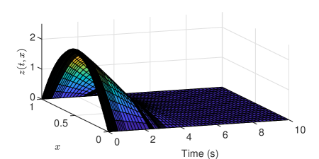
(a) State $z(t,x)$

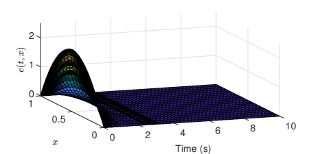
(b) Observation error $z(t,x)-\sum_{n=1}^{N}\hat{z}_{n}(t)\phi_{n}(x)$

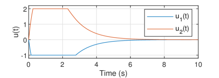
(c) Control input $u(t)$

Figure 1: Closed-loop behavior for the initial condition $z_{0}(x)=8.5x(1-x)$

V Extension to boundary measurements

Assume that $p\in\mathcal{C}^{2}([0,1])$ and consider instead of the bounded measurement operator (6) that the observation is made by either the left Dirichlet boundary measurement

$$y(t)=z(t,0)=\sum_{n\geq 1}c_{n}z_{n}(t)$$ (22)

with $c_{n}=\phi_{n}(0)$ in the case $\theta_{1}\in(0,\pi/2]$ or the left Neumann boundary measurement

$$y(t)=z_{x}(t,0)=\sum_{n\geq 1}c_{n}z_{n}(t)$$ (23)

with $c_{n}=\phi^{\prime}_{n}(0)$ in the case $\theta_{1}\in[0,\pi/2)$, where the above series expansion hold for classical solutions. We reuse the control architecture (9) and the control design procedure presented in Subsection III-A with the updated version of $c_{n}\in\mathbb{R}$. Note that the existence of classical solutions associated with initial conditions $z_{0}\in D(\mathcal{A})$ for the subsequent closed-loop system is the consequence of [23, Sec. 6.3]. After replacement of the definition of $E^{N-N_{0}}$ and $C_{1}$ by

$$E^{N-N_{0}} =\begin{bmatrix}\sqrt{\lambda_{N_{0}+1}}e_{N_{0}+1}&\ldots&\sqrt{\lambda_{N}}e_{N}\end{bmatrix}^{\top},$$

$$C_{1} =\begin{bmatrix}\frac{c_{N_{0}+1}}{\sqrt{\lambda_{N_{0}+1}}}&\ldots&\frac{c_{N+1}}{\sqrt{\lambda_{N+1}}}\end{bmatrix}$$

in the case of the Dirichlet boundary measurement (22) and by

$$E^{N-N_{0}} =\begin{bmatrix}\lambda_{N_{0}+1}e_{N_{0}+1}&\ldots&\lambda_{N}e_{N}\end{bmatrix}^{\top},$$

$$C_{1} =\begin{bmatrix}\frac{c_{N_{0}+1}}{\lambda_{N_{0}+1}}&\ldots&\frac{c_{N+1}}{\lambda_{N+1}}\end{bmatrix}$$

in the case of the Neumann boundary measurement (23), we infer that (12) holds with $F$ defined by (11) with the updated version of $C_{1}$. The main interest of this re-scaling procedure is that the matrix $\|C_{1}\|=O(1)$ as $N\rightarrow+\infty$, which will allow the application of Lemma 2; see [15] for details.

Remark 11

It can be seen that the pair $(A_{0},C_{0})$ is observable if and only if $c_{n}\neq 0$ for $1\leq n\leq N_{0}$. In the case $c_{n}=\phi_{n}(0)$ with $\theta_{1}\in(0,\pi/2]$, due to the boundary condition $\cos(\theta_{1})\phi_{n}(0)-\sin(\theta_{1})\phi_{n}^{\prime}(0)=0$, the identity $c_{n}=0$ would imply that $\phi_{n}(0)=\phi_{n}^{\prime}(0)$, giving the contradiction $\phi_{n}=0$. A similar argument applies in the case $c_{n}=\phi_{n}^{\prime}(0)$ with $\theta_{1}\in[0,\pi/2)$. Hence, in both cases, the pair $(A_{0},C_{0})$ is observable.   $\circ$

In the case of the Dirichlet boundary measurement (22), the stability analysis can now be conducted similarly to the proof of Theorem 2 by modifying the estimate of $\zeta(t)$ by $\zeta(t)^{2}\leq M_{1,\phi}\sum_{n\geq N+1}\lambda_{n}z_{n}(t)^{2}$ with $M_{1,\phi}=\sum_{n\geq N+1}\frac{\phi_{n}(0)^{2}}{\lambda_{n}}<+\infty$. We hence obtain the following result.

Theorem 3

Let $\theta_{1}\in(0,\pi/2]$, $\theta_{2}\in[0,\pi/2]$, $p\in\mathcal{C}^{2}([0,1])$ with $p>0$, $\tilde{q}\in\mathcal{C}^{0}([0,1])$, and $\ell\in(\mathbb{R}_{>0})^{m}$. Let $q\in\mathcal{C}^{0}([0,1])$ and $q_{c}\in\mathbb{R}$ be such that (4) holds with the additional constraint $q>0$. Let $b_{k}\in L^{2}(0,1)$ for $1\leq k\leq m$. Consider the reaction-diffusion system described by (3) with left Dirichlet boundary measurement (22). Let $N_{0}\geq 1$ and $\delta>0$ be given such that $-\lambda_{n}+q_{c}<-\delta<0$ for all $n\geq N_{0}+1$. Assume that for any $1\leq n\leq N_{0}$, there exists $1\leq k=k(n)\leq m$ such that $b_{n,k}\neq 0$. Let $K\in\mathbb{R}^{m\times N_{0}}$ and $L\in\mathbb{R}^{N_{0}}$ be such that $A_{0}+B_{0}K$ and $A_{0}-LC_{0}$ are Hurwitz with eigenvalues that have a real part strictly less than $-\delta<0$. For a given $N\geq N_{0}+1$, assume that there exist a symmetric positive definite $P\in\mathbb{R}^{2N\times 2N}$, $\alpha>1$, $\beta,\gamma,\mu,\kappa>0$, a diagonal positive definite $T\in\mathbb{R}^{m\times m}$, and $C\in\mathbb{R}^{m\times N_{0}}$ such that

$$\Theta_{1}(\kappa)\preceq 0,\quad\Theta_{2}\succeq 0,\quad\Theta_{3}(\kappa)\leq 0$$ (24)

where $\Theta_{1}(\kappa)$ and $\Theta_{2}$ are defined as in Theorem 1 while

$$\Theta_{3}(\kappa) =2\gamma\left\{-\left(1-\frac{1}{\alpha}\right)\lambda_{N+1}+q_{c}+\kappa\right\}+\beta M_{1,\phi}.$$

Consider the block representation $P=(P_{i,j})_{1\leq i,j\leq 4}$ with dimensions that are compatible with (10) and define

$$\mathcal{E}_{3} =\bigg{\{}z\in D(\mathcal{A}):\begin{bmatrix}\pi_{N_{0}}z\\ \pi_{N_{0},N}\mathcal{A}^{1/2}z\end{bmatrix}^{\top}\begin{bmatrix}P_{2,2}&P_{2,4}\\ P_{4,2}&P_{4,4}\end{bmatrix}\begin{bmatrix}\pi_{N_{0}}z\\ \pi_{N_{0},N}\mathcal{A}^{1/2}z\end{bmatrix}$$

$$\hskip 68.28644pt+\gamma\|\mathcal{R}_{N}\mathcal{A}^{1/2}z\|_{L^{2}}^{2}<\frac{1}{\mu}\bigg{\}}.$$ (25)

Then, considering the closed-loop system composed of the plant (3) with left Dirichlet boundary measurement (22) and the control law (9), there exists $M>0$ such that for any initial condition $z_{0}\in\mathcal{E}_{3}$ and with a zero initial condition of the observer (i.e., $\hat{z}_{n}(0)=0$ for all $1\leq n\leq N$), the system trajectory satisfies $\|z(t,\cdot)\|_{H^{1}}^{2}+\sum_{n=1}^{N}\hat{z}_{n}(t)^{2}\leq Me^{-2\kappa t}\|z_{0}\|_{H^{1}}^{2}$ for all $t\geq 0$. Moreover, for any fixed $\kappa\in(0,\delta]$, the above constraints are always feasible for $N$ large enough.

In the case of the Neumann boundary measurement (23), the stability analysis can also be conducted similarly to the proof of Theorem 2 by modifying the estimate of $\zeta(t)$ by $\zeta(t)^{2}\leq M_{2,\phi}(\epsilon)\sum_{n\geq N+1}\lambda_{n}^{3/2+\epsilon}z_{n}(t)^{2}$ with $M_{2,\phi}(\epsilon)=\sum_{n\geq N+1}\frac{\phi_{n}^{\prime}(0)^{2}}{\lambda_{n}^{3/2+\epsilon}}<+\infty$ for any given $\epsilon\in(0,1/2]$. We hence obtain the following result.

Theorem 4

Let $\theta_{1}\in[0,\pi/2)$, $\theta_{2}\in[0,\pi/2]$, $p\in\mathcal{C}^{2}([0,1])$ with $p>0$, $\tilde{q}\in\mathcal{C}^{0}([0,1])$, and $\ell\in(\mathbb{R}_{>0})^{m}$. Let $q\in\mathcal{C}^{0}([0,1])$ and $q_{c}\in\mathbb{R}$ be such that (4) holds with the additional constraint $q>0$. Let $b_{k}\in L^{2}(0,1)$ for $1\leq k\leq m$. Consider the reaction-diffusion system described by (3) with left Neumann boundary measurement (23). Let $N_{0}\geq 1$ and $\delta>0$ be given such that $-\lambda_{n}+q_{c}<-\delta<0$ for all $n\geq N_{0}+1$. Assume that for any $1\leq n\leq N_{0}$, there exists $1\leq k=k(n)\leq m$ such that $b_{n,k}\neq 0$. Let $K\in\mathbb{R}^{m\times N_{0}}$ and $L\in\mathbb{R}^{N_{0}}$ be such that $A_{0}+B_{0}K$ and $A_{0}-LC_{0}$ are Hurwitz with eigenvalues that have a real part strictly less than $-\delta<0$. For a given $N\geq N_{0}+1$, assume that there exist a symmetric positive definite $P\in\mathbb{R}^{2N\times 2N}$, $\alpha>1$, $\beta,\gamma,\mu,\kappa>0$, $\epsilon\in(0,1/2]$, a diagonal positive definite $T\in\mathbb{R}^{m\times m}$, and $C\in\mathbb{R}^{m\times N_{0}}$ such that

$$\Theta_{1}(\kappa)\preceq 0,\quad\Theta_{2}\succeq 0,\quad\Theta_{3}(\kappa)\leq 0,\quad\Theta_{4}\geq 0$$ (26)

where $\Theta_{1}(\kappa)$ and $\Theta_{2}$ are defined as in Theorem 1 while

$$\Theta_{3}(\kappa) =2\gamma\left\{-\left(1-\frac{1}{\alpha}\right)\lambda_{N+1}+q_{c}+\kappa\right\}+\beta M_{2,\phi}(\epsilon)\lambda_{N+1}^{1/2+\epsilon}$$

$$\Theta_{4} =2\gamma\left\{1-\frac{1}{\alpha}\right\}-\dfrac{\beta M_{2,\phi}(\epsilon)}{\lambda_{N+1}^{1/2-\epsilon}}.$$

Consider the block representation $P=(P_{i,j})_{1\leq i,j\leq 4}$ with dimensions that are compatible with (10) and define

$$\mathcal{E}_{4} =\bigg{\{}z\in D(\mathcal{A}):\begin{bmatrix}\pi_{N_{0}}z\\ \pi_{N_{0},N}\mathcal{A}z\end{bmatrix}^{\top}\begin{bmatrix}P_{2,2}&P_{2,4}\\ P_{4,2}&P_{4,4}\end{bmatrix}\begin{bmatrix}\pi_{N_{0}}z\\ \pi_{N_{0},N}\mathcal{A}z\end{bmatrix}$$

$$\hskip 68.28644pt+\gamma\|\mathcal{R}_{N}\mathcal{A}^{1/2}z\|_{L^{2}}^{2}<\frac{1}{\mu}\bigg{\}}.$$ (27)

Then, considering the closed-loop system composed of the plant (3) with left Neumann boundary measurement (23) and the control law (9), there exists $M>0$ such that for any initial condition $z_{0}\in\mathcal{E}_{4}$ and with a zero initial condition of the observer (i.e., $\hat{z}_{n}(0)=0$ for all $1\leq n\leq N$), the system trajectory satisfies $\|z(t,\cdot)\|_{H^{1}}^{2}+\sum_{n=1}^{N}\hat{z}_{n}(t)^{2}\leq Me^{-2\kappa t}\|z_{0}\|_{H^{1}}^{2}$ for all $t\geq 0$. Moreover, for any fixed $\kappa\in(0,\delta]$, the above constraints are always feasible for $N$ large enough.

Remark 12

Even if Theorems 3 and 4 address the case of left boundary measurements, right boundary measurements can also be conducted similarly. This is also the case of in-domain measurements of the type $y(t)=z(t,\xi)$ and $y(t)=z_{x}(t,\xi)$ for some $\xi\in(0,1)$. In that case, one need to explicitly check that the pair $(A_{0},C_{0})$ is observable, which holds true if an only if $\phi_{n}(\xi)\neq 0$ for all $1\leq n\leq N_{0}$ in the case of a Dirichlet measurement while $\phi_{n}^{\prime}(\xi)\neq 0$ for all $1\leq n\leq N_{0}$ in the case of a Neumann measurement.   $\circ$

VI Conclusion

This paper has studied the output feedback stabilization of a reaction-diffusion PDEs by means of bounded control inputs. The control strategy takes the form of a finite-dimensional controller. The reported stability analysis takes advantage of Lyapunov functionals along with a classical generalized sector condition that is commonly used in the analysis of finite-dimensional saturated systems. The obtained sets of constraints ensuring the stability of the closed-loop system take an explicit form and have been shown to be feasible when the order of the observer is large enough. An explicit subset of the domain of attraction of the closed-loop system has been derived.

Technical lemma

The statement of the following Lemma is borrowed from [15, Appendix] and generalizes a result presented in [11].

Lemma 2

Let $n,m,N\geq 1$, $M_{11}\in\mathbb{R}^{n\times n}$ and $M_{22}\in\mathbb{R}^{m\times m}$ Hurwitz, $M_{12}\in\mathbb{R}^{n\times m}$, $M_{14}^{N}\in\mathbb{R}^{n\times N}$, $M_{24}^{N}\in\mathbb{R}^{m\times N}$, $M_{31}^{N}\in\mathbb{R}^{N\times n}$, $M_{33}^{N},M_{44}^{N}\in\mathbb{R}^{N\times N}$, and

$$F^{N}=\begin{bmatrix}M_{11}&M_{12}&0&M_{14}^{N}\\ 0&M_{22}&0&M_{24}^{N}\\ M_{31}^{N}&0&M_{33}^{N}&0\\ 0&0&0&M_{44}^{N}\end{bmatrix}.$$

We assume that there exist constants $C_{0},\kappa_{0}>0$ such that $\|e^{M_{33}^{N}t}\|\leq C_{0}e^{-\kappa_{0}t}$ and $\|e^{M_{44}^{N}t}\|\leq C_{0}e^{-\kappa_{0}t}$ for all $t\geq 0$ and all $N\geq 1$. Moreover, we assume that there exists a constant $C_{1}>0$ such that $\|M_{14}^{N}\|\leq C_{1}$, $\|M_{24}^{N}\|\leq C_{1}$, and $\|M_{31}^{N}\|\leq C_{1}$ for all $N\geq 1$. Then there exists a constant $C_{2}>0$ such that, for any $N\geq 1$, there exists a symmetric matrix $P^{N}\in\mathbb{R}^{n+m+2N}$ with $P^{N}\succ 0$ such that $(F^{N})^{\top}P^{N}+P^{N}F^{N}=-I$ and $\|P^{N}\|\leq C_{2}$.

References

- [1] M. J. Balas, “Finite-dimensional controllers for linear distributed parameter systems: exponential stability using residual mode filters,” Journal of Mathematical Analysis and Applications, vol. 133, no. 2, pp. 283–296, 1988.
- [2] D. S. Bernstein and A. N. Michel, “A chronological bibliography on saturating actuators,” 1995.
- [3] H. Brézis, Functional analysis, Sobolev spaces and partial differential equations. Springer, 2011, vol. 2, no. 3.
- [4] P. Campo and M. Morari, “Robust control of processes subject to saturation nonlinearities,” Computers & Chemical Engineering, vol. 14, no. 4-5, pp. 343–358, 1990.
- [5] J.-M. Coron and E. Trélat, “Global steady-state controllability of one-dimensional semilinear heat equations,” SIAM Journal on Control and Optimization, vol. 43, no. 2, pp. 549–569, 2004.
- [6] R. Curtain, “Finite-dimensional compensator design for parabolic distributed systems with point sensors and boundary input,” IEEE Transactions on Automatic Control, vol. 27, no. 1, pp. 98–104, 1982.
- [7] S. Dubljevic, N. H. El-Farra, P. Mhaskar, and P. D. Christofides, “Predictive control of parabolic pdes with state and control constraints,” International Journal of Robust and Nonlinear Control: IFAC-Affiliated Journal, vol. 16, no. 16, pp. 749–772, 2006.
- [8] N. H. El-Farra, A. Armaou, and P. D. Christofides, “Analysis and control of parabolic pde systems with input constraints,” Automatica, vol. 39, no. 4, pp. 715–725, 2003.
- [9] J. M. Gomes da Silva Jr and S. Tarbouriech, “Antiwindup design with guaranteed regions of stability: an lmi-based approach,” IEEE Transactions on Automatic Control, vol. 50, no. 1, pp. 106–111, 2005.
- [10] W. Kang and E. Fridman, “Boundary control of delayed ODE-heat cascade under actuator saturation,” Automatica, vol. 83, pp. 252–261, 2017.
- [11] R. Katz and E. Fridman, “Constructive method for finite-dimensional observer-based control of 1-D parabolic PDEs,” Automatica, vol. 122, p. 109285, 2020.
- [12] I. Lasiecka and T. I. Seidman, “Strong stability of elastic control systems with dissipative saturating feedback,” Systems & Control Letters, vol. 48, no. 3-4, pp. 243–252, 2003.
- [13] H. Lhachemi and C. Prieur, “Feedback stabilization of a class of diagonal infinite-dimensional systems with delay boundary control,” IEEE Transactions on Automatic Control, vol. 66, no. 1, pp. 105–120, 2020.
- [14] ——, “Finite-dimensional observer-based PI regulation control of a reaction-diffusion equation,” IEEE Transactions on Automatic Control, 2021, in press.
- [15] ——, “Finite-dimensional observer-based boundary stabilization of reaction-diffusion equations with either a Dirichlet or Neumann boundary measurement,” Automatica, vol. 135, p. 109955, 2022.
- [16] H. Lhachemi, C. Prieur, and R. Shorten, “In-domain stabilization of block diagonal infinite-dimensional systems with time-varying input delays,” IEEE Transactions on Automatic Control, vol. 66, no. 12, pp. 6017–6024, 2021.
- [17] H. Lhachemi, C. Prieur, and E. Trélat, “PI regulation of a reaction-diffusion equation with delayed boundary control,” IEEE Transactions on Automatic Control, vol. 66, no. 4, pp. 1573–1587, 2020.
- [18] S. Marx, V. Andrieu, and C. Prieur, “Cone-bounded feedback laws for m-dissipative operators on hilbert spaces,” Mathematics of Control, Signals, and Systems, vol. 29, no. 4, pp. 1–32, 2017.
- [19] S. Marx, E. Cerpa, C. Prieur, and V. Andrieu, “Global stabilization of a korteweg–de vries equation with saturating distributed control,” SIAM Journal on Control and Optimization, vol. 55, no. 3, pp. 1452–1480, 2017.
- [20] B. Mavkov, E. Witrant, and C. Prieur, “Distributed control of coupled inhomogeneous diffusion in tokamak plasmas,” IEEE Transactions on Control Systems Technology, vol. 27, no. 1, pp. 443–450, 2017.
- [21] A. Mironchenko, C. Prieur, and F. Wirth, “Local stabilization of an unstable parabolic equation via saturated controls,” IEEE Transactions on Automatic Control, vol. 66, no. 5, pp. 2162–2176, 2020.
- [22] Y. Orlov, “On general properties of eigenvalues and eigenfunctions of a Sturm–Liouville operator: comments on “ISS with respect to boundary disturbances for 1-D parabolic PDEs”,” IEEE Transactions on Automatic Control, vol. 62, no. 11, pp. 5970–5973, 2017.
- [23] A. Pazy, Semigroups of linear operators and applications to partial differential equations. Springer Science & Business Media, 2012, vol. 44.
- [24] C. Prieur, S. Tarbouriech, and J. M. Gomes da Silva Jr, “Wave equation with cone-bounded control laws,” IEEE Transactions on Automatic Control, vol. 61, no. 11, pp. 3452–3463, 2016.
- [25] D. L. Russell, “Controllability and stabilizability theory for linear partial differential equations: recent progress and open questions,” SIAM Review, vol. 20, no. 4, pp. 639–739, 1978.
- [26] Y. Sakawa, “Feedback stabilization of linear diffusion systems,” SIAM journal on control and optimization, vol. 21, no. 5, pp. 667–676, 1983.
- [27] M. Slemrod, “Feedback stabilization of a linear control system in Hilbert space with an a priori bounded control,” Mathematics of Control, Signals and Systems, vol. 2, no. 3, pp. 265–285, 1989.
- [28] Y. Smagina, O. Nekhamkina, and M. Sheintuch, “Stabilization of fronts in a reaction-diffusion system: Application of the Gershgorin theorem,” Industrial & engineering chemistry research, vol. 41, no. 8, pp. 2023–2032, 2002.
- [29] S. Tarbouriech, G. Garcia, J. M. da Gomes da Silva Jr, and I. Queinnec, Stability and stabilization of linear systems with saturating actuators. Springer Science & Business Media, 2011.
- [30] S. Wang, M. Diagne, and J. Qi, “Delay-adaptive predictor feedback control of reaction-advection-diffusion PDEs with a delayed distributed input,” IEEE Transactions on Automatic Control, 2021.
- [31] Y. Wang, K. Xu, Y. Kang, H. Wang, F. Wang, and A. Avram, “Regional influenza prediction with sampling twitter data and PDE model,” International journal of environmental research and public health, vol. 17, no. 3, p. 678, 2020.
- [32] L. Zaccarian and A. R. Teel, Modern anti-windup synthesis: control augmentation for actuator saturation. Princeton University Press, 2011.