Abstract

Effective field theories (EFT) are commonly used to parameterize effects of BSM physics in vector boson scattering (VBS). For Wilson coefficients which are large enough to produce presently observable effects, the validity range of the EFT represents only a fraction of the energy range covered by the LHC, however. In order to shed light on possible extrapolations into the high energy region, a class of UV-complete toy models, with extra SU(2) multiplets of scalars or of fermions with vector-like weak couplings, is considered. By calculating the Wilson coefficients up to energy-dimension eight, and full one-loop contributions to VBS due to the heavy multiplets, the EFT approach, with and without unitarization at high energy, is compared to the perturbative prediction. For high multiplicities, e.g. nonets of fermions, the toy models predict sizable effects in transversely polarized VBS, but only outside the validity range of the EFT. At lower energies, dimension-eight operators are needed for an adequate description of the models, providing another example that dimension-eight can be more important than dimension-six operators. A simplified VBFNLO implementation is used to estimate sensitivity of VBS to such BSM effects at the LHC. Unitarization captures qualitative features of the toy models at high energy but significantly underestimates signal cross sections in the threshold region of the new particles.

1 Introduction

With over 300 fb^-1 of data collected at the LHC, vector boson scattering processes (VBS) have become important testing grounds for the non-abelian structure of electroweak interactions, as described by the Standard Model (SM). While early measurements of the CMS and ATLAS collaborations firmly established the presence of these electroweak $qq\to qqVV$ signals [1, 2], at a level as predicted by the SM, the focus is now shifting to precise comparisons between data and theoretical predictions and the search for possible signals beyond the SM. Possible deviations in the three- and four-vector-boson-couplings as compared to SM predictions, so called anomalous triple gauge couplings (aTGC) or anomalous quartic gauge couplings (aQGC) have received particular attention [2, 3].

Anomalous couplings are conveniently described within an effective field theory (EFT) framework [4, 5, 6, 7] with operators of energy dimension $d=6$ and 8 such as

$$\mathcal{L}_{EFT} =\sum_{d=6}^{\infty}\sum_{i}\frac{{f_{i}}^{(d)}}{\Lambda^{d-4}}{O_{i}}^{(d)}=\sum_{i}\frac{{f_{i}}^{(6)}}{\Lambda^{2}}{O_{i}}^{(6)}+\sum_{i}\frac{{f_{i}}^{(8)}}{\Lambda^{4}}{O_{i}}^{(8)}+...$$

$$=\frac{f_{WWW}}{\Lambda^{2}}\text{Tr}\left(\tensor{\hat{W}}{{}^{\mu}_{\nu}}\tensor{\hat{W}}{{}^{\nu}_{\rho}}\tensor{\hat{W}}{{}^{\rho}_{\mu}}\right)+\dots$$

$$+\frac{f_{T_{0}}}{\Lambda^{4}}\text{Tr}\left(\hat{W}^{\mu\nu}\hat{W}_{\mu\nu}\right)\text{Tr}\left(\hat{W}^{\alpha\beta}\hat{W}_{\alpha\beta}\right)+\dots$$

$$+\frac{f_{M_{0}}}{\Lambda^{4}}\hbox{Tr}\left[{\hat{W}}_{\mu\nu}{\hat{W}}^{\mu\nu}\right]\times\left[\left(D_{\beta}\Phi\right)^{\dagger}D^{\beta}\Phi\right]+\dots$$

$$+\frac{f_{S_{0}}}{\Lambda^{4}}\left[\left(D_{\mu}\Phi\right)^{\dagger}D_{\nu}\Phi\right]\times\left[\left(D^{\mu}\Phi\right)^{\dagger}D^{\nu}\Phi\right]\,+\dots.$$ (1)

Here $\Phi$ represents the Higgs doublet field ($\Phi=(0,v+h)/\sqrt{2}$ in the unitary gauge), ${\hat{W}}_{\mu\nu}$ is the SU(2) field strength tensor, and the scale of new physics is generically called $\Lambda$. For a process with typical momentum transfer $Q^{2}$, deviations from SM amplitudes will generally scale like $(Q/\Lambda)^{d-4}$ or $(v/\Lambda)^{d-4}$ within the validity range of the EFT, which is set by $Q^{2}<\Lambda^{2}$, and, thus, dimension-6 operators are expected to dominate at the LHC. The dynamics of the new physics may, however, suppress the Wilson coefficients $f_{i}/\Lambda^{2}$ of dimension-6 operators such that the leading effects arise from dimension-8 operators. A simple example is the Euler-Heisenberg Lagrangian [8], where a term analogous to $f_{T_{0}}$ in Eq. (1) exists, due to the electron loop producing a 4-photon interaction, while a $f_{WWW}$-like term is forbidden by Furry’s theorem, i.e. the fact that the photon is C-odd. As we will see later, such a suppression of aTGCs vs. aQGCs, due to Furry’s theorem, does indeed occur for simple extensions of the SM.

A second consideration is whether the operators in the EFT Lagrangian are loop induced or whether they may occur due to tree level effects of the underlying UV-complete model. While terms such as $f_{S_{0}}$ in Eq. (1) can arise from tree level scalar exchange in e.g. a two-Higgs-doublet model, the appearance of field strength tensors in the effective Lagrangian generally points to a loop origin of the effective interaction. The concomitant suppression by loop factors $g^{2}/(16\pi^{2})$ tends to substantially reduce the phenomenological importance of such operators [9], at least when they are competing with SM tree level effects. One might thus be tempted to ignore any loop induced operators in the study of VBS, arguing that loop induced effects are too small to be observed above sizable SM contributions to VBS. We will show that this assumption, while warranted for a large class of models, can be false when high multiplicities of the additional fields occur in the UV physics.

New charged particles are expected to first appear in direct pair production at colliders, or, indirectly, in the simplest $n$-point functions which can be probed. Already three decades ago, de Rujula and collaborators asked “Does LEP-1 obviate LEP-2?” [10], i.e. does the non-observation of new physics in 2-point functions, via the $S$, $T$, $U$ parameters of LEP-1, exclude the observation of anomalies in $W$-pair production at LEP-2. Translated to the present, the question arises whether the measurement of quartic couplings in VBS can lead to a first BSM signal, even though the $\bar{q}q\to VV$ vector boson pair production processes are observed at the LHC with much higher statistics and are also known better theoretically, with the availability of e.g. NNLO QCD corrections [11, 12, 13, 14, 15]. An additional scalar resonance would be an obvious example for the power of VBS. However, we will show that for large isospin multiplets also purely transverse aQGCs, like the $f_{T}$ term in Eq. (1), may be more sensitive probes of new physics than aTGCs, because aQGCs are enhanced by an additional factor of isospin-squared. Of course, very large isospin representations will push models out of the perturbative domain, a tension which we will probe by unitarity considerations.

Typically, Wilson coefficients of dimension-8 operators, which are large enough to be observable in present data, will produce scattering amplitudes which exceed unitarity bounds within the energy range of the LHC. Not taking into account the resulting unitarity limits on cross sections results in overly stringent constraints on Wilson coefficients. Accordingly, recent LHC analyses take unitarity constraints into account in their extraction of limits on aQGC (see e.g. Refs. [2, 3]). Unfortunately, unitarization procedures for VBS amplitudes such as the T-matrix approach of Refs. [16, 17, 18] or the $T_{u}$-model of Ref. [19] are arbitrary to a significant degree, introducing model dependence in the measurement of the Wilson coefficients of an EFT. A comparison of unitarized cross sections with predictions of UV-complete toy models can help to make the unitarization procedures more realistic.

In this paper we address the above questions by confronting the EFT description of the transverse, dimension-6 $f_{WWW}$- and dimension-8 $f_{T}$-type operators in Eq. (1) with a fairly generic class of UV-complete models with additional matter fields in arbitrary weak isospin representations. The model, given by the addition to the SM of $(2J_{R}+1)$-dimensional SU(2) multiplets of heavy scalars and/or heavy non-chiral Dirac fermions, is further specified in Section 2.1. At the one-loop level, which is summarized in Section 2.2, its low energy manifestation is described by an EFT Lagrangian involving (derivatives of) SU(2) field strengths, i.e. only transverse operators contribute. The relevant operators are introduced in Section 2.3. In Section 2.4 we present the Wilson coefficients of all EFT terms up to energy dimension eight. Many of them have been measured in various experiments and the existing bounds are translated into exclusions of $(J_{R},M_{R})$ combinations in Section 2.5, with $M_{R}$ denoting the mass of the heavy scalars or fermions. The resulting amplitudes for VBS processes diverge at high energy, proportional up to $s^{2}/M_{R}^{4}$ where $\sqrt{s}$ is the c.m. energy of the $VV\to VV$ VBS process. In order to assess the validity range of the EFT description, we also calculate, in Section 3, the full one-loop corrections to the $VV\to VV$ scattering amplitudes which arise from the heavy new matter fields. Performing a partial wave analysis, their trajectory around the Argand circle is analyzed in Section 3.1 and we are thus able to specify for which isospin $J_{R}$ a perturbative description is still justified. At the limit of this perturbative range, we compare the full one-loop corrected cross sections for $VV\to VV$ scattering with the EFT approximation in Section 3.2. We find good agreement of the two approaches only for $\sqrt{s}\lesssim 1.3M_{R}$, as is to be expected.

While the above results are obtained in a simplified setting, neglecting the hypercharge coupling $g^{\prime}$ and considering on-shell scattering only, an approximate implementation for the full $qq\to qqVV$ processes within the VBFNLO Monte Carlo program [20, 21] is presented in Section 4. On the theoretical side, this allows for a more realistic comparison of the full model with its EFT approximation, at dimension-8 level, and with the unitarized replacement of the EFT in the $T_{u}$ model of Ref. [19]. Also here, good agreement between the three approaches is found for $\sqrt{s}<1.3M_{R}$, very large deviations are seen in the threshold region for pair production of the heavy particles ($M_{R}<\sqrt{s}<2M_{R}$), and qualitatively acceptable agreement of the $T_{u}$-model with the full one-loop corrected results occurs well above pair production threshold. The VBFNLO implementation also allows to compare the expected VBS signals of high isospin fermion or scalar multiplets with LHC data. Finally, conclusions are presented in Section 5.

2 The toy model and its EFT

As a set of minimal, ultraviolet-complete models, we consider the addition of heavy fermionic or scalar SU$(2)_{L}$ multiplets to the SM. These new degrees of freedom are assumed to couple through the SU$(2)_{L}$ gauge interaction only, i.e. they are color singlets and have vanishing hypercharge. In addition, they are assumed to have negligible Yukawa or $\Phi^{4}$ couplings to the SM Higgs doublet field and, thus, they do not mix with the other particles of the SM.

2.1 Definition and description of the toy model

To be specific, and in order to fix the notation, we consider Dirac fermions $\Psi$ with mass $M_{F}$ or complex scalars $\Phi$ with mass $M_{S}$, which transform under a generic SU$(2)_{L}$ representation $R$ described by the generators $t_{R}^{a}$. The representation $R$ is specified by its isospin, $J_{R}$, i.e. each multiplet has $(2J_{R}+1)$ components and $t_{R}^{a}t_{R}^{a}=J_{R}(J_{R}+1)$. Since the covariant derivatives of the new, hypercharge-zero fields contain SU$(2)_{L}$ gauge fields only,

$$D_{\mu}=\partial_{\mu}+igt_{R}^{a}W^{a}_{\mu}\,,$$ (2)

no relevant information will be lost in our loop calculations and EFT considerations by simplifying the model to a pure SU$(2)_{L}$ gauge theory, i.e. we restrict most of the discussion to the SU$(2)_{L}$ limit of the electroweak sector of the SM, where the hypercharge coupling $g^{\prime}$ of U$(1)_{Y}$ is set to zero.

Within this approximation, the covariant derivative of the Higgs doublet field is $\hat{D}_{\mu}=\partial_{\mu}+ig\frac{\tau^{a}}{2}W_{\mu}^{a}$, with the Pauli matrices $\tau^{a}$, and the SU$(2)_{L}$ field-strength tensor is defined through

$$\hat{W}^{\mu\nu}=\left[\hat{D}^{\mu},\hat{D}^{\nu}\right]=ig\frac{\tau^{a}}{2}\left(\partial^{\mu}W^{a\nu}-\partial^{\nu}W^{a\mu}-g\epsilon^{abc}W^{b\mu}W^{c\nu}\right)=ig\frac{\tau^{a}}{2}W^{a\mu\nu}\,.$$ (3)

Suppressing the SM fermions and the Higgs potential, the relevant toy-model Lagrangian can be written as

$$\mathcal{L}= \frac{1}{2}\left(\partial_{\mu}H\right)^{2}-\frac{m_{H}^{2}}{2}H^{2}-\frac{1}{2}\text{Tr}\left(\hat{W}^{\mu\nu}\hat{W}_{\mu\nu}\right)+\frac{m_{W}^{2}}{2}\left(\sum_{a=1}^{3}W^{a}_{\mu}W^{a\mu}\right)\left(1+\frac{H}{v}\right)^{2}$$

$$+\bar{\Psi}\left(i\gamma_{\mu}D^{\mu}-M_{F}\right)\Psi+(D^{\mu}\Phi)^{\dagger}(D_{\mu}\Phi)-M_{S}{}^{2}\Phi^{\dagger}\Phi\,.$$ (4)

The first line corresponds to the well-known SM Lagrangian of the gauge and Higgs sector in the unitary gauge, albeit with equal $W$ and $Z$ masses, $m_{W}=m_{Z}=gv/2$. The second line of Eq. (4) comprises the new particles and their interactions with the gauge fields, which give rise to familiar expressions for the Feynman rules. Our loop calculations will involve internal lines of only the new fermions or scalars. Thus, results in the unitary gauge, outlined above, are identical to those of a more general $R_{\xi}$ gauge. The new fermions’ gauge couplings are assumed to be non-chiral and therefore their mass, $M_{F}$, can be chosen arbitrarily (and large) prior to spontaneous symmetry breaking of the SU$(2)_{L}$. In principle our toy model can host various fermionic and scalar multiplets without mass mixing. However, this will be irrelevant for our phenomenological discussion.

Our toy model is closely related to new-physics solutions of problems that remain open in the SM, like an explanation of neutrino masses or dark matter: Large fermionic and scalar SU$(2)_{L}$ multiplets up to quintets that couple among each other and to the lepton sector of the SM are known to provide an explanation of neutrino masses [22, 23, 24, 25, 26, 27, 28]. However, we are interested in the impact of such SU$(2)_{L}$ multiplets on vector boson scattering only and thus allow the new particles to couple to the SM only through the gauge coupling of SU$(2)_{L}$. Such large multiplets can also contain a dark matter candidate, as the lightest particle in the multiplet spectrum can be stable. Our model coincides with a class of minimal dark matter models [29, 30, 31], which range from SU$(2)_{L}$ triplets up to septets (see Ref. [32] for a review).

Embedding the heavy matter fields into the full SM, i.e. including the U$(1)_{Y}$ gauge field, the mass degeneracy of the additional SU$(2)_{L}$ multiplets at lowest-order in perturbation theory is lifted at the one-loop level, due to the mass splitting between photon, $W$ and $Z$. As an example, and in agreement with the literature [29], for a $J_{F}=4$ fermion nonet of zero hypercharge, the differences in mass of the charged states with respect to the neutral state are given by $\Delta m^{4\pm}=m_{\Psi^{4\pm}}-m_{\Psi^{0}}=2.7$ GeV, $\Delta m^{3\pm}=1.5$ GeV, $\Delta m^{2\pm}=0.66$ GeV and $\Delta m^{\pm}=0.166$ GeV. Thus, cascade decays from the heavier, charged states to the neutral, stable state proceed through far off-shell gauge bosons that result in very soft leptons and pions. If on the one hand the decay length of the charged states is short enough that they decay within the interaction region and do not result in a charged track in the detector, but on the other hand the final state leptons and pions are still soft enough, then such dark matter models are very hard to be probed at the LHC.

A thorough discussion of the current exclusions of a minimal dark matter quintet, based on LHC searches, can be found in Ref. [33], including projections for the high-luminosity runs. Expected exclusion bounds range to quintet masses up to $750$ GeV for integrated luminosities of $3$ ab^-1. Going beyond quintets, i.e. beyond $J_{R}=2$, results in the existence of additional charged states, that are pair-produced with large cross sections that rise proportional to $J_{R}(J_{R}+1)$ [29]. It is also known that the minimal dark matter model needs masses of the dark matter candidate in the range of $10$ TeV [34] in order to achieve the correct relic abundance, such that for lighter masses, as discussed in this paper, only a fraction of the observed abundance can be explained by the neutral, stable particle of the minimal dark matter model. Alternatively, extensions with additional singlet states [35] are discussed in the literature, which, however, change the collider phenomenology substantially without impacting too much the discussion carried out in this paper. Because the collider constraints can always be avoided by somewhat increasing the mass parameters $M_{F}$ or $M_{S}$, we omit a more detailed discussion of direct exclusion limits from existing collider searches, as this is not the focus of the present paper.

2.2 One-loop corrections to gauge-boson vertices, isospin factors and renormalization

The additional SU$(2)_{L}$ multiplets contribute to various observables at the one-loop level. Here we focus on contributions to VBS, which enter through propagator, three- and four-boson vertex corrections. In practice we use FeynCalc [36, 37] for the handling of Dirac structures, we regularize ultraviolet divergences through dimensional regularization and express our findings in terms of Passarino-Veltman integrals [38, 39] to obtain numerical results. We refrain from showing the explicit, rather lengthy expressions for the corrections to the three- and four-gauge-boson vertices. Instead, we here concentrate on the general structure of the one-loop contributions, including their representation dependence.

We start with the vacuum polarization. For the fermion case only a single diagram contributes. For the scalar case a second diagram involving the four-particle vertex needs to be added. As the propagator corrections are purely transverse, they generically take the form

$$\vbox{\hbox{\includegraphics[page=2,scale={0.8}]{figures/Renormalization2W}}}+\vbox{\hbox{\includegraphics[page=3,scale={0.8}]{figures/Renormalization2W}}}=i\delta^{ab}\left(p^{2}g^{\mu\nu}-p^{\mu}p^{\nu}\right)T_{S}\Pi_{S}(p^{2},M_{S}^{2})\,$$ (5)

for the scalar case and similarly, replacing $T_{S}\Pi_{S}(p^{2},M_{S}^{2})$ by $T_{F}\Pi_{F}(p^{2},M_{F}^{2})$ for the fermion loop. For the diagrams involving two three-particle vertices the isospin factor is $\text{Tr}\left(t_{R}^{a}t_{R}^{b}\right)=T_{R}\delta^{ab}$ while the scalar diagram with the four-particle vertex has $\text{Tr}\left(\{t_{R}^{a},t_{R}^{b}\}\right)=2T_{R}\delta^{ab}$. Therein $T_{R}=T_{F}$ or $T_{S}$ is the index of the representation, given by $T_{R}=\frac{1}{3}\left[J_{R}(J_{R}+1)(2J_{R}+1)\right]$ for an isospin $J_{R}$ representation. The explicit form of the propagator corrections is given by

$$\Pi_{F}(p^{2},M_{F}^{2})=-\frac{g^{2}}{16\pi^{2}}\frac{4}{9p^{2}}\left[6M_{F}^{2}-p^{2}-6A_{0}(M_{F}^{2})+3(2M_{F}^{2}+p^{2})B_{0}(p^{2},M_{F}^{2},M_{F}^{2})\right]\,,$$

$$\Pi_{S}(p^{2},M_{S}^{2})=\frac{g^{2}}{16\pi^{2}}\frac{1}{9p^{2}}\left[12M_{S}^{2}-2p^{2}-12A_{0}(M_{S}^{2})+3(4M_{S}^{2}-p^{2})B_{0}(p^{2},M_{S}^{2},M_{S}^{2})\right]\,.$$ (6)

These expressions can be expanded in small momenta $p^{2}$ motivated by $p^{2}\sim m_{W}^{2}\ll M_{F}^{2},M_{S}^{2}$. As we employ dimensional regularization, working in $d=4-2\epsilon$ dimensions, we parameterize the divergences in terms of $\Delta_{\epsilon}=\frac{1}{\epsilon}-\gamma_{E}+\log(4\pi)$. The propagator corrections then turn into

$$\Pi_{F}(0,M_{F}^{2})=-\frac{g^{2}}{16\pi^{2}}\frac{4}{3}\left[\Delta+\log\left(\frac{\mu^{2}}{M_{F}^{2}}\right)\right]\,,$$

$$\Pi_{S}(0,M_{S}^{2})=-\frac{g^{2}}{16\pi^{2}}\frac{1}{3}\left[\Delta+\log\left(\frac{\mu^{2}}{M_{S}^{2}}\right)\right]\,,$$ (7)

where $\mu$ denotes the renormalization scale. It is therefore clear that choosing an $\overline{\text{MS}}$ scheme with $\mu=M_{F},M_{S}$ leads practically to an on-shell scheme with almost vanishing propagator corrections, such that electroweak precision data are not significantly impacted by the extra degrees of freedom.

We now turn our attention to the three-boson vertex. The result is generically of the form

$$\left(\vbox{\hbox{\includegraphics[page=1,scale={0.7}]{figures/Renormalization3W}}}+\text{permutations}\right)=i\epsilon^{abc}T_{F}\Gamma_{3,F}^{\mu\nu\rho}(p_{1},p_{2},p_{3},M_{F}^{2})\,$$ (8)

for heavy fermions, and analogously for scalars. Here “permutations” of the external gauge bosons refers to the Feynman graph with the opposite direction of the fermion arrow. For the three-boson vertex correction in the scalar case, all diagrams involving the $WW\Phi\Phi$ seagull vertex vanish individually because, among other reasons, their isospin factor $\text{Tr}\left(t_{R}^{a}\{t_{R}^{b},t_{R}^{c}\}\right)$ is zero. The sum of the depicted diagrams, on the other hand, carries an isospin factor $\text{Tr}\left(t_{R}^{a}[t_{R}^{b},t_{R}^{c}]\right)=iT_{R}\epsilon^{abc}$.

For the scalar case, the one-loop corrections to the four-gauge boson vertex take the form

$$\left(\vbox{\hbox{\includegraphics[page=3,scale={0.8}]{figures/Renormalization4W}}}+\vbox{\hbox{\includegraphics[page=4,scale={0.8}]{figures/Renormalization4W}}}+\vbox{\hbox{\includegraphics[page=2,scale={0.8}]{figures/Renormalization4W}}}+\text{permutations}\right)$$

$$+\left(\vbox{\hbox{\includegraphics[page=5,scale={0.8}]{figures/Renormalization4W}}}+\text{$t$- and $u$-type}\right)=\tilde{\Gamma}_{4,S}^{\mu\nu\alpha\beta,abcd}(p_{1},p_{2},p_{3},p_{4},M_{S}^{2},J_{S})\,,$$ (9)

while the corresponding heavy fermion contribution, $\tilde{\Gamma}_{4,F}^{\mu\nu\alpha\beta,abcd}(p_{1},p_{2},p_{3},p_{4},M_{F}^{2},J_{F})$ is given by a box-diagram analogous to the one shown, and its permutations. Above, the three permutations for the scalar one-loop graphs involving two four-particle vertices are labeled $s$-, $t$- and $u$-type diagram. For all diagrams we get traces over four generators, which generically result in

$$\text{Tr}\left(t_{R}^{a}t_{R}^{b}t_{R}^{c}t_{R}^{d}\right)= \frac{1}{15}T_{R}(3C_{2,R}-1)\left(\delta^{ab}\delta^{cd}+\delta^{ac}\delta^{bd}+\delta^{ad}\delta^{bc}\right)$$

$$+\frac{1}{6}T_{R}\left(\delta^{ab}\delta^{cd}-2\delta^{ac}\delta^{bd}+\delta^{ad}\delta^{bc}\right)\,.$$ (10)

Here, $T_{R}=\frac{1}{3}\left[J_{R}(J_{R}+1)(2J_{R}+1)\right]$ is the index, and $C_{2,R}=J_{R}(J_{R}+1)$ is the quadratic casimir of a representation. Eq. (10) separates the isospin symmetric part proportional to $T_{R}(3C_{2,R}-1)$, which is the only contribution to pure $ZZ\rightarrow ZZ$ scattering, from terms coming from products of $\epsilon$ tensors. Alternatively, all one-loop corrections can be sorted into terms proportional to $T_{R}$ only and terms proportional to $C_{2,R}T_{R}$, which provides the full isospin dependence. As a consequence, numerical evaluations can be performed for a fixed mass choice and can then easily be reweighted to any representation $R$. We use this procedure in VeBoS and our implementation in VBFNLO.

We now turn our attention to the renormalization of ultraviolet divergences. Since we are only considering $n$-point functions of the SU$(2)_{L}$ gauge fields which are transverse, as in Eq. (5), only the $\text{Tr}\left(\hat{W}^{\mu\nu}\hat{W}_{\mu\nu}\right)$ term in Eq. (4) can produce the necessary counter terms, via the renormalization of the gauge fields and the coupling constant. Denoting the renormalization constants between the bare Lagrangian parameters (with subscript $0$) and the physical parameters as

$$W_{0}^{a\mu}=\sqrt{Z_{3}}W^{a\mu},\qquad g_{0}=Z_{g}g\,,$$

the renormalization constants of the three and four gauge-boson vertices are given by $Z_{3W}=Z_{g}Z_{3}^{3/2}$ and $Z_{4W}=Z_{g}^{2}Z_{3}^{2}$, respectively. Writing $Z_{i}=1+\delta_{i}$, we obtain $\delta_{3W}=\delta_{g}+\frac{3}{2}\delta_{3}$ and $\delta_{4W}=2\delta_{g}+2\delta_{3}$, which defines the counter-terms for the three and four gauge-boson vertices, respectively. The counter-term of the propagator reads $\delta_{2W}=\delta_{3}$. It directly follows from the vacuum polarization in Eq. (7) that in the $\overline{\text{MS}}$ scheme the field renormalization constant $\delta_{3}$ is given by

$$\delta_{3}=-g^{2}\Delta_{\epsilon}\left(\sum_{F}n_{F}\frac{T_{F}}{12\pi^{2}}+\sum_{S}n_{S}\frac{T_{S}}{48\pi^{2}}\right)\,,$$ (11)

assuming $n_{F}$ and $n_{S}$ copies of a fermionic and scalar multiplet with isospin $J_{F}$ and $J_{S}$, respectively. From the ultraviolet divergence of the three gauge-boson vertex we obtain

$$\left(\delta_{g}+\frac{3}{2}\delta_{3}\right) =-g^{2}\Delta_{\epsilon}\left(\sum_{F}n_{F}\frac{T_{F}}{12\pi^{2}}+\sum_{S}n_{S}\frac{T_{S}}{48\pi^{2}}\right)=\delta_{3}$$ (12)

and, therefore, the renormalization constant of the SU$(2)_{L}$ coupling is given by $\delta_{g}=-\frac{1}{2}\delta_{3}$. It is easy to check that indeed the now fully determined counter term to the four gauge-boson vertex, namely $\delta_{4W}=2(\delta_{g}+\delta_{3})=\delta_{3}$, also cancels the divergence of the corresponding one-loop corrections to gauge-boson four-point functions.

2.3 Effective-field theory description

Considering the low-energy expansion of the now finite two-, three- and four-point functions of the gauge bosons, we can derive the contributions of additional heavy SU$(2)_{L}$ multiplets to the EFT Lagrangian

$$\mathcal{L}_{EFT}=\sum_{d=6}^{\infty}\sum_{i}\frac{{f_{i}}^{(d)}}{\Lambda^{d-4}}{O_{i}}^{(d)}\,,$$ (13)

i.e. we can now determine the Wilson coefficients $f_{i}/\Lambda^{2}$ and $f_{i}/\Lambda^{4}$ of the dimension-6 and dimension-8 operators which are relevant for VBS in our concrete model.

By construction, the SU$(2)_{L}$ gauge bosons are the only SM particles which couple via the heavy fermions or scalars and which can, at the one-loop level, appear as fields in the effective Lagrangian. Gauge invariance then implies that we can restrict the EFT Lagrangian to operators which contain the SU$(2)_{L}$ field strength tensor $\hat{W}^{\mu\nu}$ of Eq. (3) or its commutator with covariant derivatives. For a description of vector boson scattering we need vacuum polarization effects (dimension-4 operators and higher), anomalous triple-gauge couplings (dimension-6 and -8 operators) and anomalous quartic-gauge couplings (dimension-8 operators).

The dimension-4 operator is unique and given by

$$O_{WW} =\text{Tr}\left(\hat{W}^{\mu\nu}\hat{W}_{\mu\nu}\right)\,.$$ (14)

It is already part of the SM kinetic term. Since it receives contributions from the additional SU$(2)_{L}$ multiplets it is explicitly listed here. However, as discussed in the last section, it disappears as a result of renormalization. As a basis for the dimension-6 operators, following Ref. [5], we choose

$$O_{WWW} =\text{Tr}\left(\tensor{\hat{W}}{{}^{\mu}_{\nu}}\tensor{\hat{W}}{{}^{\nu}_{\rho}}\tensor{\hat{W}}{{}^{\rho}_{\mu}}\right)\,,$$

$$O_{DW} =\text{Tr}\left([\hat{D}_{\alpha},\hat{W}^{\mu\nu}][\hat{D}^{\alpha},\hat{W}_{\mu\nu}]\right)\,.$$ (15)

Our focus is on the dimension-8 operators which first appear as aQGC in vector boson scattering, and which involve four field-strength tensors, namely

$$O_{T_{0}} =\text{Tr}\left(\hat{W}^{\mu\nu}\hat{W}_{\mu\nu}\right)\text{Tr}\left(\hat{W}^{\alpha\beta}\hat{W}_{\alpha\beta}\right)\,,$$

$$O_{T_{1}} =\text{Tr}\left(\hat{W}^{\mu\nu}\hat{W}_{\alpha\beta}\right)\text{Tr}\left(\hat{W}^{\alpha\beta}\hat{W}_{\mu\nu}\right)\,,$$

$$O_{T_{2}} =\text{Tr}\left(\hat{W}^{\mu\nu}\hat{W}_{\nu\alpha}\right)\text{Tr}\left(\hat{W}^{\alpha\beta}\hat{W}_{\beta\mu}\right)\,,$$

$$O_{T_{3}} =\text{Tr}\left(\hat{W}^{\mu\nu}\hat{W}^{\alpha\beta}\right)\text{Tr}\left(\hat{W}_{\nu\alpha}\hat{W}_{\beta\mu}\right)\,.$$ (16)

Here we follow the notation of Refs. [7, 41, 19, 42]. However, since our definition of $\hat{W}^{\mu\nu}$ includes the coupling factor $ig$, the operators in Eq. (16) contain an overall factor $g^{4}$ as compared to the Éboli convention of Refs. [7, 41]. Please note that $O_{T_{3}}$ is a non-vanishing, linearly independent operator which was missing in previous discussions and, therefore, is also not experimentally constrained explicitly. We refer to the four operators in Eq. (16) as $T$-operators.

For three field-strength tensors in combination with covariant derivatives, seven operators can be written down which are, however, related through integration-by-parts for the covariant derivative, the Jacobi identity for covariant derivatives, and $\hat{W}^{\mu\nu}=\left[\hat{D}^{\mu},\hat{D}^{\nu}\right]$. Our set of independent operators is then given by

$$O_{DWWW_{0}} =\text{Tr}\left([\hat{D}_{\alpha},\tensor{\hat{W}}{{}^{\mu}_{\nu}}][\hat{D}^{\alpha},\tensor{\hat{W}}{{}^{\nu}_{\rho}}]\tensor{\hat{W}}{{}^{\rho}_{\mu}}\right)\,,$$

$$O_{DWWW_{1}} =\text{Tr}\left([\hat{D}_{\alpha},\tensor{\hat{W}}{{}^{\mu}{}^{\nu}}][\hat{D}_{\beta},\tensor{\hat{W}}{{}_{\mu}{}_{\nu}}]\tensor{\hat{W}}{{}^{\alpha}{}^{\beta}}\right)\,.$$ (17)

For the case of two field-strength tensors in combination with covariant derivatives we pick

$$O_{D2W}=\text{Tr}\left([\hat{D}_{\alpha},[\hat{D}^{\alpha},\hat{W}^{\mu\nu}]][\hat{D}_{\beta},[\hat{D}^{\beta},\hat{W}_{\mu\nu}]]\right)\,,$$ (18)

as, again, other combinations are not linearly independent.

The above choice of basis is by no means unique but simply driven by the physics of the underlying theory. Looking at the dimension-6 operators one could make an argument for using the Warsaw Basis [6] as this could make comparisons easier and gives more direct access to exclusion limits for the Wilson coefficients. Rewriting the $O_{DW}$ operator using integration-by-parts, the commutator for the covariant derivatives as well as the Jacobi identity for covariant derivatives, one arrives at 

$$O_{DW}=2\text{Tr}\left([\hat{D}_{\alpha},\hat{W}^{\alpha\mu}][\hat{D}^{\nu},\hat{W}_{\nu\mu}]\right)-4\,O_{WWW}\,.$$ (19)

At this point we can use the equations of motion for the $W$-field twice:

$$[\hat{D}^{\alpha},\hat{W}_{\alpha\mu}]=\frac{ig^{2}\,\tau^{I}}{4}\left(i\phi^{\dagger}\tau^{I}D_{\mu}\phi-i\left(D_{\mu}\phi\right)^{\dagger}\tau^{I}\phi+\bar{l}\gamma_{\mu}\tau^{I}l+\bar{q}\gamma_{\mu}\tau^{I}q\right)+\mathcal{O}(\frac{1}{\Lambda^{2}}).$$ (20)

Here the last term accounts for corrections to the equations of motion due to the presence of $O_{DW}$ and $O_{WWW}$ which are of order $\frac{1}{\Lambda^{2}}$. This leaves us with four types of terms: operators containing four Higgs fields, the ones containing fermionic currents, and also terms of order $\frac{1}{\Lambda^{2}}$ and $\frac{1}{\Lambda^{4}}$ of which only the latter may be neglected as they are of order $\frac{1}{\Lambda^{6}}$ when including the Wilson coefficient of $O_{DW}$. The terms with four Higgs fields can again be rewritten by using relations for the SU$(2)_{L}$ generators as well as the equations of motion for the Higgs field and one finds

$$O_{DW}=-g^{3}\,{\rm{O}}_{W}-\frac{3g^{4}}{4}{\rm{O}}_{\phi\square}+\frac{g^{4}m_{H}^{2}}{2}\left(\phi^{\dagger}\phi\right)^{2}-2g^{4}\lambda{\rm{O}}_{\phi}+{\rm{O}}_{\psi^{2}\phi^{2}D}+{\rm{O}}_{\psi^{4}}+\mathcal{O}(\frac{1}{\Lambda^{2}})\,,$$ (21)

where the operators on the r.h.s., with $\phi$ representing the SM Higgs doublet field, are written in the Warsaw basis. Here $\psi$ stands for either leptons or quarks. The last two operators are just symbolizing the class of additional operators that can appear following the conventions in Ref. [6]. Individual terms in this new set now give local corrections to Higgs and fermionic observables that, at the one-loop level, are not present for the BSM heavy matter fields which we consider. Therefore, these corrections have to cancel each other when calculating amplitudes for physical processes in our new physics model. This also implies that any exclusion limits for Wilson coefficients are only useful when provided with full error correlations. With this in mind it becomes apparent that there is no advantage in using the Warsaw basis over the basis defined by Eqs. (15)-(18).

2.4 Wilson coefficients due to additional SU$(2)_{L}$ multiplets

After presenting the full EFT Lagrangian we can map our concrete model onto the Wilson coefficients at low energies by integrating out the heavy new degrees of freedom. Again we assume to have $n_{F}$ and $n_{S}$ copies of fermionic and scalar multiplets with isospin $J_{F}$ and $J_{S}$, respectively. We expand the one-loop corrections in small momenta with respect to the mass scale of the new heavy degrees of freedom, i.e. $\frac{p_{i}\cdot p_{j}}{M^{2}}\ll 1$, which for the Wilson coefficients originating from propagator corrections results in

$$f_{WW} =\sum_{F}n_{F}\frac{T_{F}}{24\pi^{2}}\left(\Delta_{\epsilon}+\log\left(\frac{\mu^{2}}{M_{F}^{2}}\right)\right)+\sum_{S}n_{S}\frac{T_{S}}{96\pi^{2}}\left(\Delta_{\epsilon}+\log\left(\frac{\mu^{2}}{M_{S}^{2}}\right)\right)\,,$$ (22)

$$\frac{f_{DW}}{\Lambda^{2}} =\sum_{F}n_{F}\frac{T_{F}}{120\pi^{2}M_{F}^{2}}+\sum_{S}n_{S}\frac{T_{S}}{960\pi^{2}M_{S}^{2}}\,,$$ (23)

$$\frac{f_{D2W}}{\Lambda^{4}} =\sum_{F}n_{F}\frac{T_{F}}{1120\pi^{2}M_{F}^{4}}+\sum_{S}n_{S}\frac{T_{S}}{13440\pi^{2}M_{S}^{4}}\,.$$ (24)

We continue to expand the three gauge boson-vertex corrections in a similar manner in small momenta, which leads to

$$\frac{f_{WWW}}{\Lambda^{2}} =\sum_{F}n_{F}\frac{13T_{F}}{360\pi^{2}M_{F}^{2}}+\sum_{S}n_{S}\frac{T_{S}}{360\pi^{2}M_{S}^{2}}\,,$$ (25)

$$\frac{f_{DWWW_{0}}}{\Lambda^{4}} =\sum_{F}n_{F}\frac{2T_{F}}{105\pi^{2}M_{F}^{4}}+\sum_{S}n_{S}\frac{T_{S}}{1120\pi^{2}M_{S}^{4}}\,,$$ (26)

$$\frac{f_{DWWW_{1}}}{\Lambda^{4}} =\sum_{F}n_{F}\frac{T_{F}}{630\pi^{2}M_{F}^{4}}+\sum_{S}n_{S}\frac{T_{S}}{4032\pi^{2}M_{S}^{4}}\,.$$ (27)

Finally, the Wilson coefficients of the $T$-operators are given by

$$\frac{f_{T_{0}}}{\Lambda^{4}} =\sum_{F}n_{F}\frac{\left(-14C_{2,F}+1\right)T_{F}}{10080\pi^{2}M_{F}^{4}}+\sum_{S}n_{S}\frac{\left(7C_{2,S}-2\right)T_{S}}{40320\pi^{2}M_{S}^{4}}\,,$$ (28)

$$\frac{f_{T_{1}}}{\Lambda^{4}} =\sum_{F}n_{F}\frac{\left(-28C_{2,F}+13\right)T_{F}}{10080\pi^{2}M_{F}^{4}}+\sum_{S}n_{S}\frac{\left(14C_{2,S}-5\right)T_{S}}{40320\pi^{2}M_{S}^{4}}\,,$$ (29)

$$\frac{f_{T_{2}}}{\Lambda^{4}} =\sum_{F}n_{F}\frac{\left(196C_{2,F}-397\right)T_{F}}{25200\pi^{2}M_{F}^{4}}+\sum_{S}n_{S}\frac{\left(14C_{2,S}-23\right)T_{S}}{50400\pi^{2}M_{S}^{4}}\,,$$ (30)

$$\frac{f_{T_{3}}}{\Lambda^{4}} =\sum_{F}n_{F}\frac{\left(98C_{2,F}+299\right)T_{F}}{25200\pi^{2}M_{F}^{4}}+\sum_{S}n_{S}\frac{\left(7C_{2,S}+16\right)T_{S}}{50400\pi^{2}M_{S}^{4}}\,.$$ (31)

As discussed previously, all UV divergences of propagator-, triangle-, and box-diagrams are contained in the coefficient of the field-strength-square operator $O_{WW}$ and, hence, disappear upon renormalization of the SU$(2)_{L}$ gauge coupling $g$ and the gauge boson fields.

Some additional remarks are in order:

• The isospin factors of propagator and three-boson-vertex corrections are given by $T_{R}$ and thus rise with $J_{R}^{3}$. The Wilson coefficients of the $T$-operators, on the other hand, are enhanced by an additional casimir factor, i.e. they rise as $J_{R}^{5}$, enhancing their importance over the dimension-6 operators for high isospin.

• Individual operators in the scalar case are more suppressed than for heavy fermions of the same mass and isospin.

• The Wilson coefficients of the $T$-operators $f_{T_{0}}$ and $f_{T_{1}}$ receive opposite sign contributions from heavy scalars vs. heavy fermions, which can induce cancellations between $T$-operator contributions to e.g. VBS cross sections. $f_{T_{2}}$ changes its sign at $J_{R}\sim 1$ for both the fermionic and scalar multiplets.

2.5 Confronting Wilson coefficients with experiment

Having obtained the low-energy EFT of the general model, we next investigate whether specific model realizations are compatible with experimental limits on four-fermion contact terms, anomalous triple- and anomalous quartic-gauge couplings. Since we are only interested in rough estimates for our toy model, we restrict the discussion to the single multiplet realization and determine bounds in the $(J_{R},M_{R})$ parameter space.

The insertion of $O_{DW}$ into the gauge boson propagator of a $q\bar{q}\to l^{+}l^{-}$ amplitude scales like

$$\frac{1}{p^{2}-m_{W}^{2}}\times p^{4}\frac{f_{DW}}{\Lambda^{2}}\times\frac{1}{p^{2}-m_{W}^{2}}\quad\sim\quad\frac{f_{DW}}{\Lambda^{2}}$$

at high energy and, thus, reduces to a flavor universal, dimension-6 four-fermion interaction which affects left-chiral amplitudes only. Writing the coefficient of the $\bar{Q}_{L}\gamma^{\mu}Q_{L}\,\bar{L}\gamma_{\mu}L$ EFT operator as $2\pi\,\eta_{LL}/\Lambda_{LL}^{2}$ one finds $\eta_{LL}=-1$ and

$$\Lambda^{2}_{LL}=2\pi\,\frac{240\pi^{2}M_{F}^{2}}{g^{4}T_{F}}\qquad{\rm or}\qquad\Lambda^{2}_{LL}=2\pi\,\frac{1920\pi^{2}M_{S}^{2}}{g^{4}T_{S}}\,,$$ (32)

for a single fermion or scalar multiplet in the loop, respectively. In the EFT approximation, experimental bounds on four-fermion contact terms, such as recent ATLAS measurements [43], can thus be turned into the lower limits on $M_{R}^{2}/T_{R}$ which are shown in Fig. 1.

aTGCs are typically measured in the LEP parameterization, where the effective $WWV$-coupling parameters $\Delta g_{1}$, $\Delta\kappa$ and $\lambda$ are used [44]. $\lambda$ parameterizes transverse weak boson interactions and thus is the one of primary interest here. The loop-corrections of our model contribute both to propagators, via the dimension-6 operator $O_{DW}$, and to triple gauge-boson vertices, via both $O_{DW}$ and $O_{WWW}$. In the $\bar{q}q\to WW$ amplitude, in the SU$(2)_{L}$ limit, the former is equivalent to an energy dependent $\Delta g_{1}=\Delta\kappa$ contribution, while the latter are best captured after the operator redefinition in Eq. (19). One finds

$$\lambda=\frac{3m_{W}^{2}g^{2}}{2}\left(\frac{f_{WWW}}{\Lambda^{2}}-4\frac{f_{DW}}{\Lambda^{2}}\right)\, =g^{2}\,m_{W}^{2}\,\left(\sum_{F}n_{F}\frac{T_{F}}{240\pi^{2}M_{F}^{2}}-\sum_{S}n_{S}\frac{T_{S}}{480\pi^{2}M_{S}^{2}}\right)\,,$$ (33)

$$\Delta\kappa=\Delta g_{1}=2g^{2}m_{W}^{2}\frac{f_{DW}}{\Lambda^{2}}\,\frac{s-2m_{W}^{2}}{s-m_{W}^{2}} \approx g^{2}\,m_{W}^{2}\,\left(\sum_{F}n_{F}\frac{T_{F}}{60\pi^{2}M_{F}^{2}}+\sum_{S}n_{S}\frac{T_{S}}{480\pi^{2}M_{S}^{2}}\right)\,.$$ (34)

Going beyond the SU$(2)_{L}$ limit, the $\lambda$-aTGC can easily be compared to existing data, via $\lambda_{\gamma}=\lambda_{Z}=\lambda$. The $\Delta g_{1}$ and $\Delta\kappa$ contributions would appear as process dependent form-factors, however, which are constrained at a similar level as the induced $\lambda$-aTGC.

Coefficient	limit without unitar.	channel	limit with unitarity cut	channel
$\eta_{LL}=-1$: $\Lambda_{LL}$	$26.0$ TeV	$pp\to l^{+}l^{-}X$	–	–
$\lambda$	$[-6.5,6.6]\cdot 10^{-3}$	$WV\to l\nu J$	–	–
$g^{4}\frac{f_{T_{0}}}{\Lambda^{4}}$	$[-0.24,0.22]\,$TeV-4	$ZZ$	$[-1.1,1.6]\,$TeV-4	$ssWW,WZ$
$g^{4}\frac{f_{T_{1}}}{\Lambda^{4}}$	$[-0.12,0.14]\,$TeV-4	$ssWW,WZ$	$[-0.69,0.97]\,$TeV-4	$ssWW,WZ$
$g^{4}\frac{f_{T_{2}}}{\Lambda^{4}}$	$[-0.35,0.48]\,$TeV-4	$ssWW,WZ$	$[-1.6,3.1]\,$TeV-4	$ssWW,WZ$

Table 1: Experimental 95% CL bounds on four-fermion couplings [43], aTGCs [45] and aQGCs [46, 47]. The values for aQGCs from the CMS analyses are derived from leptonic decay channels in VBS processes only. aQGC bounds are presented with and without a unitarization in form of a cut at the perturbative unitarity limit of the EFT calculation. In addition, we name the channels from which the presented bounds are derived.

Table 1 summarizes relevant bounds on four-fermion couplings, aTGCs, and aQGCs. For the bounds on $T$-operators, we use the recent CMS results of Refs. [46, 47] on leptonic decay modes in VBS processes, which also take into account limitations from unitarity. Since these aQGC bounds are only specified for insertions of single EFT operators, Fig. 1 depicts the limits on the $(J_{R},M_{R})$ parameter space for each Wilson coefficient separately. Although the strong correlations between the Wilson coefficients in our model are not taken into account by this procedure, it suffices here, since we are only aiming at a rough estimate of allowed regions in the $(J_{R},M_{R})$ plane.

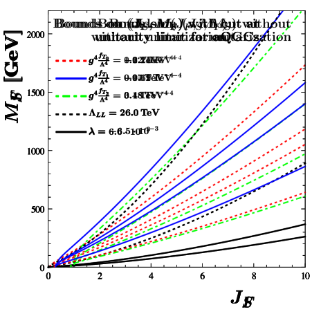
Figure 1: Translation of the experimental bounds on Wilson coefficients as in Table 1 to the $(J_{R},M_{R})$ parameter space: masses above the curves are allowed by the individual measurements. Shown are the cases of a fermion multiplet (left panel) and a scalar multiplet (right panel). For aQGCs, experimental results are derived with a step-function form-factor, cutting off the EFT prediction at the unitarity limit (see Ref. [3] for details).

The figures indicate that a measurement of aQGCs has higher potential to find effects of the BSM physics considered here than aTGC measurements. To be more concrete, we consider the cases of a fermion with $J_{F}=4$ and of a scalar with $J_{S}=6$ in the following, values which represent maximal multiplet sizes compatible with unitarity and perturbativity limits to be discussed in Section 3.1.

For the fermion multiplet, the strongest bound is associated with searches for $qqll$ contact terms, disfavoring masses below $700\,$GeV. Somewhat weaker, at $M_{F}>540\,$GeV, are bounds derived from limits on the dimension-8 $T_{1}$-operator, which do take into account unitarity constraints. Restrictions via the other $T$-operators are qualitatively similar. The aQGC bounds in turn are much more stringent than the bound from the $\lambda$-aTGC, which only excludes masses below $100\,$GeV in the EFT dimension-6 approximation.

The discussion is comparable in the scalar case. The bounds in the $(J_{S},M_{S})$ parameter plane are less stringent, however, as anticipated from the higher numerical suppression in the Wilson coefficients. Again all $T$-operator bounds appear to be stronger than the aTGC bounds, even when including unitarity considerations only for the former (see Fig. 1, right), making VBS more promising for the investigation of this model than vector boson pair production. For $J_{S}=6$, the bound on the coefficient of the $T_{1}$ operator disfavors masses below $470\,$GeV, while searches for $qqll$ contact terms appear to imply a slightly weaker bound of $M_{S}>430$ GeV.

Guided by these constraints, we will use $J_{F}=4,\,M_{F}=600$ GeV and $J_{S}=6,\,M_{S}=600$ GeV as benchmark points in the remainder of the paper to illustrate consequences for VBS at the LHC. For fermion multiplets, $M_{F}=600$ GeV appears to be in slight tension with $qqll$ contact term limits. However, additional BSM effects which we do not consider, like an extra $Z^{\prime}$, might ameliorate the tension. Since we are not explicitly proposing a viable BSM model, but are rather interested in generic features for VBS, we prefer a common mass for fermions and scalars in our subsequent discussions.

Another reason for taking the $(J_{R},M_{R})$ bounds derived from EFT considerations only as indicative is the concern that the experimental EFT analyses, especially for the $qqll$ contact terms and the aQGC, are largely based on data with dilepton or $VV$ invariant masses above 1 TeV. For our large multiplet model the EFT approximation cannot be expected to hold for invariant masses of the order of the threshold energy of $2\,M_{R}$ or larger.

As a case in point, let us have a brief look at $q\bar{q}\to l^{+}l^{-}$ production at the LHC, from which $qqll$ contact term bounds are derived. In this process and at 1-loop level, our model only influences the vector boson propagator. The Dyson-resummation of the on-shell renormalized propagator corrections, which follow from Eqs. (5) and (6), leads to

$$D(p^{2})=\frac{-i}{p^{2}-m_{W,pole}^{2}-p^{2}\Pi_{R,pole}}\,$$ (41)

for $W^{\pm}$ exchange between purely left-chiral fermions. For comparison with $l^{+}l^{-}$ data, $\gamma$-$Z$ propagator mixing needs to be considered and the BSM contributions are somewhat diluted by U$(1)_{Y}$ hypercharge contributions which, in our toy model, are left unchanged with respect to the SM. The results are shown in Fig. 2 where the ratio of the dilepton invariant mass distribution in our toy model as compared to the SM is displayed for $M_{R}=600$ GeV and a selection of isospins. Also shown, for the $J_{F}=4$ and $J_{S}=6$ benchmark points, is the BSM to SM ratio in the EFT approximation, considering the equivalent dimension-6 $qqll$ contact term only.

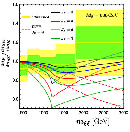
Figure 2: Ratio of the modified Drell-Yan invariant mass distribution to the SM expectation at the LHC. For a multiplet mass of $M_{R}=600$ GeV, the left (right) panel considers the effect of four different isospin choices of a fermion (scalar) multiplet. The colored bands, based on the results of Ref. [48], provide an estimate of present experimental sensitivity at the $1\sigma$ and $2\sigma$ level.

While BSM effects are negligible in the $m_{ll}<m_{R}/2$ region (below 1.5% for $J_{F}=4$ and well below 1% for $J_{S}=6$), sizable deviations from the SM are expected at higher energies, for large isospin representations. The EFT dimension-6 approximation reproduces the full one-loop result considerably below production threshold, but it fails spectacularly above threshold. Since the bounds on $qqll$ contact terms in Table 1 heavily depend on data at $m_{ll}>2.5$ TeV, one concludes that the contact term bounds on the $(J_{R},M_{R})$ parameter plane cannot be taken at face value. However, around the production threshold, the deviations from the SM are even bigger than suggested by the EFT approximation, and a full analysis of the model should be performed in this region to extract bounds on $M_{R}$.

As a first rough approximation, we have translated the results of a recent CMS analysis of dilepton production [48] to 1- and 2-$\sigma$ error bands in Fig. 2, assuming fully correlated systematic errors between electron and muon channels and adding systematic and statistical errors in quadrature, otherwise. Inspection of Fig. 2 then suggests that for $M_{R}=600$ GeV and at 95% CL the scalar benchmark point with $J_{S}=6$ is still allowed, while strong evidence for the fermionic case with $J_{F}=4$ should have been seen already. Since we consider our setup as a toy model, and since we are primarily interested in its qualitative predictions for VBS, we postpone a more detailed analysis to future work and use the benchmark point merely for illustration in the following.

3 On-shell vector boson scattering at one-loop

The large deviations between EFT results and the full model prediction for lepton pair-production provide a strong motivation to also consider the full model for VBS predictions. For a study of its main phenomenological features, we start with a discussion of on-shell VBS. In the following we neglect the normal SM electroweak corrections, which are parametrically small compared to the contributions from extra SU$(2)_{L}$ multiplets, due to the $J_{R}^{3}$ to $J_{R}^{5}$ enhancement of the latter. Corrections from the new heavy degrees of freedom originate from the previously discussed one-loop contributions to the gauge-boson propagators and the three- and four-gauge-boson vertex functions. In terms of Feynman diagrams, for external gauge bosons in the adjoint basis ($W^{\mu}_{a_{i}}$ with $a_{i}=1,2,3$) the scattering amplitudes can be depicted as

$$\vbox{\hbox{\includegraphics[page=8,scale={0.75}]{figures/VBS}}}=\vbox{\hbox{\includegraphics[page=1,scale={0.75}]{figures/VBS}}}+\left(\vbox{\hbox{\includegraphics[page=2,scale={0.75}]{figures/VBS}}}+\vbox{\hbox{\includegraphics[page=3,scale={0.75}]{figures/VBS}}}+\text{$t$- and $u$-type}\right)$$

$$\qquad+\left(\vbox{\hbox{\includegraphics[page=4,scale={0.75}]{figures/VBS}}}+\vbox{\hbox{\includegraphics[page=5,scale={0.75}]{figures/VBS}}}+\vbox{\hbox{\includegraphics[page=6,scale={0.75}]{figures/VBS}}}+\text{$t$- and $u$-type}\right)+\vbox{\hbox{\includegraphics[page=7,scale={0.75}]{figures/VBS}}}$$

$$\qquad=i\left(\mathcal{M}_{1}\delta^{ab}\delta^{cd}+\mathcal{M}_{2}\delta^{ac}\delta^{bd}+\mathcal{M}_{3}\delta^{ad}\delta^{bc}\right)\,.$$ (42)

The last equality follows from isospin symmetry, because all isospin combinations for the four indices $a_{i}$ associated with the external gauge bosons $W^{\mu}_{a_{i}}$ can be expressed by Kronecker deltas in the adjoint space. Obviously, the reduced amplitudes $\mathcal{M}_{1}$, $\mathcal{M}_{2}$, and $\mathcal{M}_{3}$ can be obtained from each other by crossing.

In this section we consider on-shell vector boson scattering in the SU$(2)_{L}$ limit, i.e. we set $g^{\prime}=0$, which eliminates any photon contributions and leads to $Z=W^{3}$ and $m_{Z}=m_{W}=\frac{gv}{2}$, thus simplifying the scattering kinematics. Projecting the amplitude of Eq. (42) onto $Z$ bosons (with a factor $\delta^{3a_{i}}$) or $W$ bosons (with a factor $\frac{1}{\sqrt{2}}\left(\delta^{1a_{i}}\pm i\delta^{2a_{i}}\right)$ for each incoming $W^{\pm}$ or outgoing $W^{\mp}$), one finds

$$\mathcal{M}\left(W^{\pm}W^{\pm}\rightarrow W^{\pm}W^{\pm}\right) =\mathcal{M}_{2}+\mathcal{M}_{3}\,,$$ (43a)

$$\mathcal{M}\left(W^{\pm}Z\rightarrow W^{\pm}Z\right) =\mathcal{M}_{2}\,,$$ (43b)

$$\mathcal{M}\left(W^{\pm}W^{\mp}\rightarrow W^{\pm}W^{\mp}\right) =\mathcal{M}_{1}+\mathcal{M}_{2}\,,$$ (43c)

$$\mathcal{M}\left(W^{\pm}W^{\mp}\rightarrow ZZ\right) =\mathcal{M}_{1}\,,$$ (43d)

$$\mathcal{M}\left(ZZ\rightarrow ZZ\right) =\mathcal{M}_{1}+\mathcal{M}_{2}+\mathcal{M}_{3}\,.$$ (43e)

As indicated by the absence of double vertex insertions in Eq. (42), our full amplitudes correspond to a coupling expansion to order $g^{4}$, with $\overline{\text{MS}}$ renormalization. Before proceeding, we need to address whether such a perturbative expansion is justified for large multiplicities, $2J_{R}+1$, which we do by a unitarity analysis of partial wave amplitudes.

3.1 Partial wave analysis of VBS amplitudes

The notation for VBS partial wave amplitudes follows Ref. [19], the results of which are implemented in VBFNLO. However, the present case is simplified by taking the SU$(2)_{L}$ limits and by considering on-shell scattering only. Exploiting angular momentum conservation, the helicity amplitudes $\mathcal{M}_{\lambda_{1}\lambda_{2}\lambda_{3}\lambda_{4}}$ of the various $VV\to VV$ processes are decomposed into coefficients of Wigner d-functions

$$\mathcal{M}_{\lambda_{1}\lambda_{2}\lambda_{3}\lambda_{4}}\left(s,\theta\right)= 8\pi\mathcal{N}_{fi}\sum_{j=max\left(|\lambda_{12}|,|\lambda_{34}|\right)}^{\infty}(2j+1)\mathcal{A}^{j}_{\lambda_{1}\lambda_{2}\lambda_{3}\lambda_{4}}\left(s\right)d^{j}_{\lambda_{12}\lambda_{34}}\left(\theta\right)\,,$$ (44)

where $\lambda_{ij}:=\lambda_{i}-\lambda_{j}$, and the normalization factor is given by $\mathcal{N}_{fi}=\frac{1}{\beta\sqrt{S_{f}S_{i}}}$, with $\beta=\sqrt{1-4m_{W}^{2}/s}$ and statistics factors $S_{f}$ or $S_{i}=1/2$ in case of two identical weak bosons. $\mathcal{N}_{fi}$ is chosen such as to simplify the constraints on the partial wave amplitudes $\mathcal{A}^{j}_{\lambda_{1}\lambda_{2}\lambda_{3}\lambda_{4}}\left(s\right)$ which follow from $S$-matrix unitarity, namely

$$2\text{Im}\left(\mathcal{A}_{\lambda_{1}\lambda_{2}\lambda_{3}\lambda_{4}}^{j}\right) \geq\sum_{n}\sum_{\lambda_{1}^{\prime},\lambda_{2}^{\prime}}\mathcal{A}_{\lambda_{3}\lambda_{4}\lambda_{1}^{\prime}\lambda_{2}^{\prime}}^{j\ast}\mathcal{A}_{\lambda_{1}\lambda_{2}\lambda_{1}^{\prime}\lambda_{2}^{\prime}}^{j}\,.$$ (45)

Here $\text{Im}\left(\mathcal{A}_{\lambda_{1}\lambda_{2}\lambda_{3}\lambda_{4}}^{j}\right)$ corresponds to the anti-hermitian part of the VBS scattering amplitude, understood as a matrix in isospin and helicity space. The sum over $n$ on the right hand side includes all relevant di-boson intermediate states. Equality in Eq. (45) would only be reached when summing over a complete set of intermediate states, including multi-particle states. For any normalized linear combination of diboson states, $|n\rangle$, the expectation value of $\mathcal{A}^{j}$ will lie within the Argand circle. In particular, this will be true for the eigenvector $|n_{\rm max}\rangle$ of the largest eigenvalue of $\text{Re}\left(\mathcal{A}^{j}\right)$ or $\text{Im}\left(\mathcal{A}^{j}\right)$. Setting

$$a^{j}=a^{j}(s)=\langle n_{\rm max}|\mathcal{A}^{j}(s)|n_{\rm max}\rangle\,,$$ (46)

which corresponds to the largest eigenvalue for a normal scattering matrix, we thus get the Argand circle condition

$$\text{Re}\left(a^{j}\right)^{2}+\left(\text{Im}\left(a^{j}\right)-1\right)^{2}\leq 1\,.$$ (47)

Since a finite perturbative expansion is only expected to fulfill this requirement approximately, e.g. an on-shell tree-level calculation remains always on the real axis and is thus never compatible with the strict requirement, the perturbative unitarity bounds are given by

$$|a^{j}|^{2}\lesssim 2\,,\quad|\text{Re}\left(a^{j}\right)|\lesssim 1\,,\quad 0\leq\text{Im}\left(a^{j}\right)\lesssim 2\,,$$ (48)

which should be understood as demanding that the eigenvalues of $\mathcal{A}^{j}$ remain close to the Argand circle in a reasonable perturbative calculation.

Figure 3: Argand diagrams for the dominating iso-singlet, $j=0$ VBS partial wave amplitudes, $a^{0}_{J_{R}}$. The left (right) panel is for a single fermion (scalar) multiplet of isospin $J_{F}$ ($J_{S}$) of mass $M_{R}=600$ GeV. Only the BSM contribution to the amplitude is shown.

When investigating the behavior of the partial wave amplitude contributions from single $(J_{R},M_{R})$ multiplets, one finds sizable effects only for the transverse helicity amplitudes $\mathcal{M}_{\text{1111}}$, $\mathcal{M}_{\text{11-1-1}}$, $\mathcal{M}_{\text{1-11-1}}$, $\mathcal{M}_{\text{1-1-11}}$ (and with corresponding parity flipped helicities). Thus it is sufficient to diagonalize the partial wave amplitudes in this restricted helicity space. This is made easier by the fact that the VBS amplitudes are also block-diagonal in the basis of total isospin of the two particle states, $|J_{2},J_{2,z}\rangle$, as we work in the $g^{\prime}=0$ limit of the SM and our BSM contributions do not break the SU$(2)_{L}$ symmetry. The dominant eigenvalue is found in the $j=0$ partial wave and corresponds to vanishing total isospin of the weak boson pair, $J_{2}=0$. Its BSM contribution is called $a^{0}$ in the following.

Figure 4: Dominating iso-singlet, $j=0$ partial wave amplitudes, $a^{0}_{J_{R}}$, as a function of the diboson center of mass energy, $\sqrt{s}$. Results are shown for the pure contribution of a single $J_{F}=4$ fermion multiplet (left panel) and of a single $J_{S}=6$ scalar multiplet (right panel), for two different masses of the extra particles, 600 GeV (blue curves) and 1000 GeV (red curves). Solid lines represent the real part of $a^{0}$, long dashed lines the imaginary part, and the short dashed lines give the purely real partial wave amplitudes in the EFT approximation. The SM contribution, at tree level, is shown for comparison.

Results are presented in Fig. 3.1 for both the fermionic multiplet (left panel) and the scalar case (right panel), for a range of isospin choices, $J_{R}$, for a multiplet mass of $M_{F}=600\,{\rm GeV}=M_{S}$, and for $200\,{\rm GeV}\,<\sqrt{s}<6000\,{\rm GeV}$. For $J_{F}\leq 4$ and $J_{S}\leq 5$, the path of $a^{0}_{J_{R}}(s)$ in the complex plane is compatible with the unitarity bounds of Eq. (48), while the scalar case with $J_{S}=6$ can be considered marginally perturbative. The strong dependence on multiplet size was to be expected because the four-boson vertex function at 1-loop order grows like $J_{R}^{5}$. In the following we would like to estimate maximal deviations from the SM which can be expected in VBS. For this purpose, the multiplet realizations of $(J_{F}=4,M_{F}=600\,$GeV$)$ and $(J_{S}=6,M_{S}=600\,$GeV$)$, chosen earlier, appear well suited for a qualitative discussion.

Fig. 3.1 shows the dependence of both the real and imaginary parts of the dominant partial wave eigenvalue, $a^{0}_{J_{R}}(s)$ on the center of mass energy of the $VV\to VV$ process. Here we fix $J_{F}=4$ for the fermion model (left panel) and $J_{S}=6$ for the extra scalar multiplet (right panel). Also the EFT prediction for $a^{0}_{J_{R}}(s)$ is shown, which is purely real and which, sufficiently below production threshold at $\sqrt{s}=2\,M_{R}$, agrees well with the full calculation. The LO SM contribution to the dominant partial wave amplitude is also depicted (gray solid line), for comparison, and because it should be added to the anomalous contribution, $a^{0}_{J_{R}}(s)$. Adding these two contributions, the resulting full partial wave amplitude stays fully within the perturbative unitarity bounds of Eq. (48) for the $J_{F}=4$ fermion multiplet and agreement for the $J_{S}=6$ scalar case is also improved at high energy. Violation of the $|\text{Re}\left(a^{j}\right)|\lesssim 1$ bound for the scalar case is actually limited to a small region around threshold, while the imaginary part of the amplitude, which dominates somewhat above threshold, is consistent with the unitarity limit. The problem with the real part of the amplitude around $\sqrt{s}=2\,M_{S}$ could be ameliorated by SU$(2)_{L}$-breaking effects, i.e. by mass splitting the multiplet and thus distributing its threshold effects over a larger energy range, by binding effects due to additional (strong) interactions of the scalar multiplet(s) or by other modifications of our toy model. This provides another argument to not discard the $J_{S}=6$ case.

In order to demonstrate the effect of different mass values, Fig. 3.1 shows results for $M_{R}=600$ GeV and $M_{R}=1000$ GeV. One finds excellent scaling: the amplitude effectively only depends on $s/M_{R}^{2}$ because the electroweak scale merely enters via the mass, $m_{W}$, of the external gauge bosons, and this gives tiny $(m_{W}/M_{R})^{2}$ corrections. This scaling behavior implies that the effects which we will demonstrate with $M_{R}=600$ GeV in the following can simply be shifted to higher energy for larger multiplet masses, with an approximately invariant ratio of BSM to SM VBS cross sections.

3.2 Cross sections for on-shell vector boson scattering

With limited statistics and sizable backgrounds for VBS events at the LHC, integrated, unpolarized VBS cross sections are sufficient for a first survey of LHC capabilities. According to Eq. (43), the information is contained in three crossing related helicity amplitudes which can be disentangled by measuring cross sections for different combinations of weak bosons: same-sign $WW$ scattering, i.e. $W^{\pm}W^{\pm}\to W^{\pm}W^{\pm}$ gives access to $\mathcal{M}_{2}+\mathcal{M}_{3}$, $WZ\to WZ$ depends on $\mathcal{M}_{2}$ only, and the $ZZ$ production processes $WW\to ZZ$ and $ZZ\to ZZ$ provide separate information on $\mathcal{M}_{1}$.

Separating SM and new physics (NP) contributions, the squared amplitude, which determines the cross section, is given by

$$\scriptstyle|\mathcal{M}_{tot}|^{2}=\underbrace{\scriptstyle|\mathcal{M}_{\text{SM}}|^{2}+2\text{Re}\left(\mathcal{M}_{\text{SM}}{\mathcal{M}_{\text{NP}}}^{\ast}\right)}_{\text{(int)}}+|\mathcal{M}_{\text{NP}}|^{2}\,.$$ (49)

Our new physics amplitude is the 1-loop contribution due to the additional heavy fermion or scalar multiplet. In a typical NLO calculation, only the interference term of the NP would be considered, together with the SM Born contribution. On the other hand, when considering anomalous couplings, frequently also the $|\mathcal{M}_{\text{NP}}|^{2}$ term is included in the cross section prediction, and this is indeed the default VBFNLO implementation of VBS. Since there are no infrared divergences in the present case, and because the purely anomalous part is necessary for a prediction of the $ZZ\to ZZ$ cross section, which due to the small Higgs boson mass has a tiny SM amplitude, we do include the $|\mathcal{M}_{\text{NP}}|^{2}$ term in our calculation, but we also show the NLO-type result in the following, dubbed “full model (int)” in the figures. An analysis of the parametrically leading terms in a perturbative expansion support the inclusion of the quadratic NP term. At large $J_{R}$, the dominant two-loop contribution is given by diagrams with an additional virtual vector boson propagator within the the multiplet loop of the four-particle vertex functions, e.g. and in the fermion case, which have representation factors of $T_{R}C_{2,R}^{2}\sim J_{R}^{7}$. On the other hand, the square of the one-loop four-particle vertex function, i.e. the $|\mathcal{M}_{\text{NP}}|^{2}$ term above, is enhanced by a factor $T_{R}^{2}C_{2,R}^{2}\sim J_{R}^{10}$ (see Eq. (10)), which would not arise until the three-loop level in the interference term.

Subsequently we present the integrated, unpolarized cross sections for scattering angles $5^{\circ}<\theta<175^{\circ}$ in the center of mass frame for the still academic $W^{\pm}W^{\pm}\to W^{\pm}W^{\pm}$, $WZ\to WZ$, $WW\to ZZ$, and $ZZ\to ZZ$ scattering processes. A more complete LHC simulation of the full $qq\to qqVV$ processes will be postponed until Section 4. The limited angular range reduces the forward and backward enhancement in the SM contribution, which is due to $t$- or $u$-channel Higgs or $W,Z$ exchange. For the new-physics contribution, we use the single multiplet realization with parameter choices discussed in Section 2.4.

Cross section results, as a function of the center-of-mass energy $\sqrt{s}=m_{VV}$, are shown in Fig. 3.2 for the case of a fermion nonet and in Fig. 3.2 for a single scalar multiplet with $J_{S}=6$.

Figure 5: Unpolarized $VV\to VV$ cross sections as a function of the COM energy $\sqrt{s}=m_{VV}$ for same-sign $WW$ scattering (upper left), $WZ$-scattering (upper right), the $WW\rightarrow ZZ$ process (lower left) and $ZZ$-scattering (lower right). BSM curves are for the case of a single fermion multiplet with $J_{F}=4,M_{F}=600\,$GeV. The diverging curves represent several EFT approximations, up to dimension-8 operators (see text for details). The “full model” with full fermion 1-loop contributions is represented by the solid blue line while “full model (int)” (dashed blue) includes the interference term in Eq. (49) only. The solid black line represents the SM expectation, in the $g^{\prime}=0$ limit.

Figure 6: Same as Fig. 3.2, but for a single scalar multiplet with $J_{S}=6,M_{S}=600\,$GeV.

A striking and well-known feature of the SM prediction is the strong suppression of the $ZZ\to ZZ$ cross section, due to the small value of $m_{H}=125$ GeV. According to Eq. (43) this implies

$$\mathcal{M}_{2;\text{SM}}+\mathcal{M}_{3;\text{SM}}\approx-\mathcal{M}_{1;\text{SM}}\,,$$ (50)

a relation which does not carry over to the NP contributions. Since $\mathcal{M}_{1}$ describes $W^{+}W^{-}\to ZZ$ while $\mathcal{M}_{2}+\mathcal{M}_{3}$ is the amplitude for same-sign $WW$ scattering, one finds opposite signs for the interference terms, $\mathcal{M}_{\text{SM}}{\mathcal{M}_{\text{NP}}}^{\ast}$, when comparing these two processes. $\mathcal{M}_{2}$ is the amplitude for $WZ$ scattering, which is related to $\mathcal{M}_{3}$ by $\theta\to\pi-\theta$ crossing. As a result one finds the same interference characteristics for $WZ$ scattering as for same-sign $WW$ scattering. Effects are larger for the latter, however, by roughly a factor of two, because the important NP amplitudes are fairly independent of scattering angle and thus add up, while the SM $t$- and $u$-channel amplitudes $\mathcal{M}_{2;\text{SM}}$ and $\mathcal{M}_{3;\text{SM}}$ peak in opposite hemispheres.

Comparing the $J_{F}=4$ fermion case in Fig. 3.2 with the $J_{S}=6$ scalar multiplet in Fig. 3.2, the effect of the scalar multiplet on cross-sections is more pronounced due to the higher representation. The constructive interference between the SM and the anomalous contribution in the $WW\to ZZ$ process (lower left) is particularly striking around the threshold for fermion or scalar pair production, which results in a peak structure centered around $\sqrt{s}=2M_{R}$. For same-sign $WW$ and for $WZ$ scattering (upper row) we see destructive interference between the SM and the anomalous contribution in the low-energy regime. This leads to a dip in the cross section at pair production threshold which, however, is soon eclipsed by the strong cross section enhancement above threshold, in particular for the scalar case. This peak above threshold is driven to a substantial degree by a large contribution from the imaginary part of the scattering amplitude, which was already evident in Fig. 3.1.

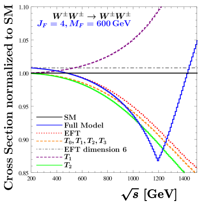
Figure 7: Ratio of the unpolarized cross sections for same-sign $WW$ scattering (left panel) and the $WW\rightarrow ZZ$ process (right panel) in the single fermion multiplet model with $(J_{F}=4,M_{F}=600\,$GeV$)$ to the corresponding SM cross section in the low energy region. In addition to the curves as in Fig. 3.2, the almost horizontal line at $\approx 1.008$ represents the result for the EFT at dimension-6 level. See text for details.

Comparing the behavior of the total amplitude squared with the NLO approximation, we observe discrepancies in the high energy regime, starting at threshold, especially for the cases of $WZ$ and same-sign $WW$ scattering. This demonstrates that our model realizations, with large isospin representations, are only marginally perturbative and might exhibit sizable higher order corrections. This is also evident for $ZZ$ scattering (lower right panels) which is clearly dominated by the anomalous contribution, i.e. the one-loop amplitudes effectively provide LO estimates, similar to $gg\to ZZ$ in the SM.

In all cases one finds good accordance between the full model and its complete EFT realization in the low-energy regime. For the EFT, four different results are shown. The complete “EFT” curves (orange dotted) contain the contributions from all dimension-6 and dimension-8 operators in Section 2.4. They are virtually indistinguishable from the orange dashed lines, dubbed $T_{0},\,,T_{1},\,,T_{2},\,,T_{3}$, which only incorporate the contributions from the dimension-8 $T$-operators. This agreement implies that the contributions from the dimension-6 operators are tiny. In addition, the violet dashed and green solid lines show predictions for an EFT, where only the $T_{1}$ or only the $T_{2}$ operator, with Wilson coefficients as given by Eqs. (31) are included. The single $T_{1}$ contribution in the fermion case exhibits the opposite interference behavior with the SM as compared to the full model and one observes strong destructive interference between the individual $T$-operators. For the scalar model, all $T$-operators interfere constructively, which can be understood by the signs of individual Wilson coefficients in Eq. (31).

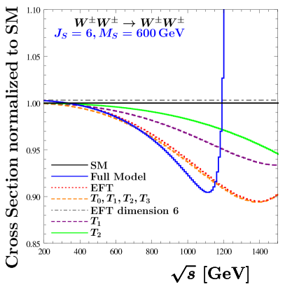
Figure 8: Same as Fig. 7, but for a single scalar multiplet with $(J_{S}=6,M_{S}=600\,$GeV$)$.

For a better evaluation of the validity of the EFT and its subsets in the low-energy region, we present in Fig. 7 and Fig. 8 the cross sections, normalized to the SM prediction, for same-sign $WW$ scattering and the $WW\rightarrow ZZ$ process. As discussed above, results for $WZ$ scattering are qualitatively the same as for same-sign $WW$ scattering.

The EFT agrees well with the full model for energies below $\sim 800\,$GeV, which is consistent with its naive validity range, given by the mass scale of the loop particle. In the fermion case, the discrepancy stays below $\sim 1\,\%$ up to 1000 GeV, but would grow with $J_{F}^{5}$. We also note that the EFT dimension-6 contribution only accounts for a slowly varying offset of less than $1\,\%$ to the pure SM cross section (gray dash-dotted line).

4 Implication for $VVjj$ events at the LHC

The analysis of the last section provided cross sections for on-shell $2\to 2$ VBS processes, in the $g^{\prime}=0$ limit, and thus was largely academic. A more realistic simulation for the LHC needs to consider the full $qQ\to qQVV$ processes, including decay of the produced electroweak gauge bosons, it needs to consider the off-shell nature of both the space-like initial and the time-like final gauge bosons, and it needs to go beyond the SU$(2)_{L}$ limit and incorporate that the $W^{3}$ is actually a linear combination of photon and $Z$ as mass eigenstates. While a full implementation of the model into VBFNLO is foreseen for the future, here we only make a first, approximate assessment of consequences for the LHC.

A prominent feature of typical VBS kinematics consists of small virtualities for all four electroweak bosons in the $V_{1}V_{2}\to V_{3}V_{4}$ subgraphs, $|p^{2}_{i}|\ll s=m_{VV}^{2}$. At such small $p_{i}^{2}$, modifications of the weak boson propagators are tiny, as evidenced by Fig. 2. Also corrections to $WWZ$ or $WW\gamma$ vertices, which appear for a high virtuality gauge boson which is radiated off a quark line in $WZjj$ and $W^{+}W^{-}jj$ production, are sub-dominant as was seen in the discussion of aTGCs in Section 2.5. The remaining BSM effects in our model then contain $V_{1}V_{2}\to V_{3}V_{4}$ subgraphs with off-shell helicity amplitudes $\mathcal{M}^{VBS}_{\lambda_{1}\lambda_{2}\lambda_{3}\lambda_{4}}(\{p_{i}^{2}\};s,t,u)$. Following Ref. [19], the BSM part, which needs to be added to the SM $qq\to qq\bar{f}_{1}f_{2}\bar{f}_{3}f_{4}$ amplitude is then given by

$$\mathcal{M}_{qq\rightarrow 4fqq}^{\rm BSM}= \prod_{i=1}^{4}\frac{1}{p_{i}^{2}-m_{V_{i}}^{2}+i\,m_{V_{i}}\,\Gamma_{V_{i}}}\sum_{\{\lambda_{i}\}}\epsilon^{*}_{J}(p_{1},\lambda_{1})\cdot J_{q\rightarrow qV_{1}}\,\,\epsilon^{*}_{J}(p_{2},\lambda_{2})\cdot J_{q\rightarrow qV_{2}}\,$$ (51)

$$\mathcal{M}^{VBS}_{\lambda_{1}\lambda_{2}\lambda_{3}\lambda_{4}}(\{p_{i}^{2}\};s,t,u)\,\,\epsilon_{J}(p_{3},\lambda_{3})\cdot J_{V_{3}\rightarrow\bar{f_{1}}f_{2}}\,\,\epsilon_{J}(p_{4},\lambda_{4})\cdot J_{V_{4}\rightarrow\bar{f_{3}}f_{4}}\,.$$

Here the $\epsilon_{J}(p_{i},\lambda_{i})$ are off-shell polarization vectors (as defined in Ref. [19]) and the $J_{q\rightarrow qV_{i}}$ and $J_{V_{i}\rightarrow\bar{f_{k}}f_{l}}$ are quark- and lepton currents. A final approximation now consists in replacing the off-shell helicity amplitudes $\mathcal{M}^{VBS}_{\lambda_{1}\lambda_{2}\lambda_{3}\lambda_{4}}(\{p_{i}^{2}\};s,t,u)=\mathcal{M}^{VBS}_{\lambda_{1}\lambda_{2}\lambda_{3}\lambda_{4}}(\{p_{i}^{2}\};s,\theta)$, determined in the VBS center-of-mass frame, by their on-shell values $\mathcal{M}^{VBS}_{\lambda_{1}\lambda_{2}\lambda_{3}\lambda_{4}}(\{m_{W}^{2}\};s,\theta)=\mathcal{M}_{\lambda_{1}\lambda_{2}\lambda_{3}\lambda_{4}}(s,\theta)$ of Eq. (44). We have verified that the above approximations are good at the 10% level by comparing on- and off-shell VBFNLO results for the dimension-8 $T$-operators [40].

In the next step we use our new VBFNLO implementation of full on-shell model amplitudes to study fiducial cross sections for the various VBS processes. We want to find out to which degree ATLAS and CMS strategies for measuring anomalous quartic gauge couplings would also reveal high multiplicity extra matter multiplets, via their impact on weak boson 4-point functions. All results are produced for a proton-proton collider with a center-of-mass energy of $13$ TeV using the MMHT2014 [50] parton distribution functions at leading order, which are linked through LHAPDF [51]. The Higgs-boson mass is set to $125.09$ GeV. For the $W$ and $Z$ boson mass VBFNLO uses $M_{W}=80.398$ GeV and $M_{Z}=91.1876$ GeV, respectively. The weak mixing angle is set to $\sin^{2}\theta_{W}=0.222646$. However we remind the reader that the inserted on-shell amplitudes are derived in the SU$(2)_{L}$ limit, in which $M_{W}=M_{Z}=81.18$ GeV. When we depict the number of events we assume an integrated luminosity of $137$ fb^-1.

4.1 Destructive interference in same-sign $WW$ and $WZ$ scattering

Figure 9: $WZ$ invariant mass (upper row) and transverse mass (lower row) distributions for VBS production of $WZjj$ events at the LHC. Three panels show expected event numbers per bin for a run 2 integrated luminosity of $137$ fb^-1 while the upper right panel is normalized to the SM. Bin width in the two left panels is $100$ GeV, while on the lower right bin size is chosen as in Ref. [3]. The considered scenario is a scalar multiplet with $J_{S}=6$ and $M_{S}=600$ GeV.

Figure 10: Same as Fig. 4.1, but for a fermionic multiplet with $J_{F}=4$ and $M_{F}=600$ GeV.

We use VBFNLO to calculate the cross sections for the electroweak processes

$$pp\to W^{\pm}Zjj\to l^{\prime\pm}\nu_{l^{\prime}}l^{\pm}l^{\mp}jj$$

$$pp\to W^{\pm}W^{\pm}jj\to l^{\pm}\nu_{l}l^{\prime\pm}\nu_{l^{\prime}}$$ (52)

with $l,l^{\prime}\in\{e,\mu\}$, which were exploited in Refs. [52, 3] to set bounds on anomalous quartic gauge couplings. In order to make a qualitative comparison with the results of Ref. [3], in particular their Fig. 6, we have implemented a very similar cut-flow. For the $WZ$ final state this cut-flow includes:

$$p_{T}^{l} >20\,\text{GeV}\,, \qquad|\eta^{e}| <2.5\,, \qquad|\eta^{\mu}| <2.4$$

$$|m_{ll}-m_{Z}| <15\,\text{GeV}\,, \qquad m_{3l} >100\,\text{GeV}\,, \qquad p_{T}^{\text{miss}} >30\,\text{GeV}$$

$$|\eta^{j}| <4.7\,, \qquad p_{T}^{j} >50\,\text{GeV}\,, \qquad|\Delta R(j,l)| >0.4$$

$$m_{jj} >500\,\text{GeV}\,, \qquad|\Delta\eta_{jj}| >2.5\,, \qquad\text{max}(z_{l}^{*}) <1.0\,.$$ (53)

Therein the abbreviation “$3l$” denotes the three-lepton system, i.e. the sum of the three lepton 4-momenta, and its invariant mass $m_{3l}$. In contrast to the CMS analysis we only simulate the flavor combination $l^{\prime}=e,l=\mu$ and as an estimate for all flavor combinations multiply our results by a factor of $4$. As a consequence we have just one cut on the transverse momentum $p_{T}^{l}$, which is chosen equal for all leptons. The cuts depicted in the last two lines of Eq. (53) are typical vector boson scattering cuts, which enhance the contribution of electroweak VBS over QCD-induced $VVjj$ events and other SM backgrounds.

$$z_{l}^{*}=|\eta^{l}-\tfrac{1}{2}(\eta^{j_{1}}+\eta^{j_{2}})|/|\Delta\eta_{jj}|$$ (54)

denotes the variable introduced in Ref. [53].

The cut-flow for the same-sign $WW$ final state is very similar: for charged leptons we merely replace the $m_{3l}$ cut by $m_{ll}>20$ GeV. Furthermore we set $\text{max}(z_{l}^{*})<0.75$. In contrast to Ref. [3] we do not have a cut on $|m_{ee}-m_{Z}|$, as we generate our result for the flavor combination $l^{\prime}=e,l=\mu$ and multiply by $2$.

We present our results primarily for the scalar case with the combination $J_{S}=6$ and $M_{S}=600$ GeV which, according to the discussion in the previous sections, may be considered a maximal plausible signal within our framework. The results for the fermionic case with $J_{F}=4$ and $M_{F}=600$ GeV, which is disfavored by Drell-Yan data, do not provide much additional insight and differ visibly only in the vicinity of the threshold peak, which is more pronounced in the scalar case. We present the number of events for an integrated luminosity of $137$ fb^-1 as a function of the invariant mass of the final state $WW$ and $WZ$ system which, however, is not accessible experimentally. Therefore, also for a direct comparison with Fig. 6 of Ref. [3], we add figures showing the transverse mass as defined there.

For the $W^{\pm}Z$ final state the results for the scalar case are depicted in Fig. 4.1 and for the fermionic case in Fig. 4.1. The $m(W^{\pm}Z)$ invariant mass distribution in Fig. 4.1 (upper left) and its ratio to the SM contribution (upper right) show destructive interference between the multiplet contribution and the SM well below the threshold at $m(W^{\pm}Z)\approx 2M_{F}=1200$ GeV. The EFT description follows this behavior until around $m(W^{\pm}Z)\approx 1000$ GeV, after which it clearly deviates from the full-model prediction. In this region of reliable EFT description the BSM effects are tiny, however, deviating from the SM by at most 1%, which renders their observation hopeless. The figures also depict the contribution from the combined dimension-8 $T_{i}$ operators only, which well coincides with the full EFT description. This exacerbates the observation in Section 3.2 that the contribution of the dimension 6 operators is sub-dominant and irrelevant for VBS in practice. The lower panels of Fig. 4.1 show the transverse momentum distribution, in which the destructive interference is not visible anymore, due to the migration of excess events at higher invariant mass into the low transverse mass region. The lower right panel reproduces the binning of the events in Fig. 6 of Ref. [3]. Comparison of the last two bins with the data (which are compatible with the SM) reveals that the full fermion model in Fig. 4.1 cannot be excluded, whereas scalar model at $J_{S}=6$ in Fig. 4.1 should have been seen with considerable significance. Similarly, the sizable signals of the non-unitarized EFT’s in the last (overflow) bin are excluded. Also shown are unitarized versions of the EFT description, following the unitarization procedure of Ref. [19], which stays closer to the full model description in both the invariant and the transverse mass distributions.

Figure 11: $WW$ invariant mass (upper row) and $llp_{T}^{\rm miss}$ transverse mass (lower row) distributions for VBS production of same-sign $WWjj$ events at the LHC. Three panels show expected event numbers per bin for a run 2 integrated luminosity of $137$ fb^-1 while the upper right panel is normalized to the SM. Bin width in the two left panels is $100$ GeV, while on the lower right bin size is chosen as in Ref. [3]. The considered scenario is a scalar multiplet with $J_{S}=6$ and $M_{S}=600$ GeV.

Figure 12: Same as Fig. 4.1, but for a fermionic multiplet with $J_{F}=4$ and $M_{F}=600$ GeV.

We continue with a description of the $W^{\pm}W^{\pm}$ final state, for which we depict the scalar case in Fig. 4.1 and the fermionic case in Fig. 4.1. The destructive interference in the invariant mass distribution is more pronounced than in the $W^{\pm}Z$ case. Unfortunately, the actually observable transverse mass distribution suffers from two final-state neutrinos which leave the detector unobserved. This again leads to the migration of a substantial fraction of high-energy events in the invariant-mass distribution to lower values of the transverse mass, which wipes out the destructive interference signal. This migration also leads to significant deviations between the full-model description and the EFT setup for all values of the transverse mass, even far below threshold, $m_{T}(W^{\pm}W^{\pm})\ll 2M_{R}$. Lastly, in the transverse-mass distribution also the unitarized EFT case is far from both the full-model description and the EFT curve, as the different behavior at high invariant-mass has a clear impact at lower values of the transverse mass. The choice of the unitarization procedure, which is arbitrary to a considerable extent, unfortunately impacts the transverse-mass distribution substantially. We note that the di-lepton invariant mass distribution would show a behavior very similar to the transverse mass, i.e. throughout the whole range of masses the full model, the EFT description and its unitarized version differ. Again the lower right panel shows the binning as performed in the left panel of Fig. 6 in Ref. [3]. In the next-to-last bin, from $850$ to $1050$ GeV in $m_{T}(W^{\pm}W^{\pm})$, all curves for the $J_{F}=4$ fermionic case are compatible with the data, whereas the measurement, with a single event in the $m_{T}(W^{\pm}W^{\pm})>1050$ GeV bin, is visibly under tension with all non-SM curves depicted in the lower right panels of Fig. 4.1 and Fig. 4.1. It is again apparent that it is much easier to exclude the EFT description compared to the full model or the unitarized EFT description.

4.2 Constructive interference in $ZZjj$ production

Within the VBFNLO framework we next consider the electroweak process

$$pp\to ZZjj\to l^{\prime+}l^{\prime-}l^{+}l^{-}jj$$

with $l,l^{\prime}\in\{e,\mu\}$, which was used in Refs. [46, 47] to bound aQGCs. For a qualitative comparison we again use a cut-flow similar to the experimental analysis, namely

$$p_{T}^{l} >20\,\text{GeV}\,, \qquad|\eta^{e}| <2.5\,, \qquad|\eta^{\mu}| <2.4$$

$$40\,\text{GeV}<m_{ll} <120\,\text{GeV}\,, \qquad|\eta^{j}| <4.7\,, \qquad p_{T}^{j} >30\,\text{GeV}$$

$$\qquad|\Delta R(j,l)| >0.3\,, \qquad m_{jj} >400\,\text{GeV}\,, \qquad|\Delta\eta_{jj}| >2.4\,.$$ (55)

We generate the flavor combination $l^{\prime}\neq l\in\{e,\mu\}$ and multiply our results with a factor of $2$, thus ignoring the problem of correctly assigning the leptons to the two $Z$ boson candidates in $4e$ or $4\mu$ events. Note that the actual experimental analysis in Ref. [46] is using a boosted decision tree, which also takes into account the $z_{l}^{*}$ variable of Eq. (54) to enhance the fraction of vector boson scattering events over QCD background events. The more recent analysis in Ref. [47] is moreover extracting the bounds not from a VBS-enhanced region, but from a larger phase space region with only $m_{jj}>100$ GeV. We stick to the VBS-enhanced region defined above for our qualitative discussion, because otherwise triple gauge boson production processes would have to be considered as well. As a consequence we cannot directly compare against Ref. [47], which would anyhow need a detailed Monte Carlo simulation of all underlying, dominant background processes.

In Fig. 13 we show the $ZZ$ invariant-mass distribution for the scalar case with $J_{S}=6$ and $M_{S}=600$ GeV which, in contrast to $WW$ or $WZ$ production, is fully accessible experimentally for $ZZ\to 4l$. While the left panel is for a constant 100 GeV bin width, the central panel uses the binning employed in Refs. [46, 47], and the ratio to the SM is shown in the right panel. In contrast to the same-sign $WW$ and $W^{\pm}Z$ final states the interference with the SM is constructive (see right panel) and the peak itself is more pronounced (see left panel). We emphasize again that a direct comparison to the experiments is non-trivial due to different regions in the phase space of the two jets. Still both the full model as well as the unitarized EFT description yield about three extra events in the last bin ($m(ZZ)>1200$ GeV), which seems well compatible with the experimental data. The qualitative behavior of the $J_{F}=4,\,M_{F}=600$ GeV model is similar to the scalar model shown. However, deviations from the SM are somewhat smaller, with a single excess event expected in the last bin.

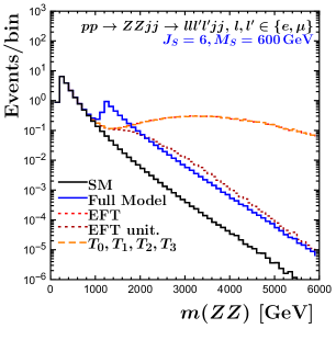
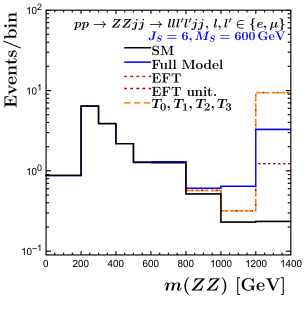
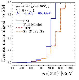
Figure 13: Diboson invariant mass distributions for $ZZjj$ VBS events at the LHC. Shown are events per $100$ GeV bin (left), events per bin, sized as in Refs. [46, 47] (middle), each for an integrated luminosity of $137$ fb^-1, and cross section normalized to the SM (right). The considered scenario is a fermionic multiplet with $J_{S}=6$ and $M_{S}=600$ GeV. VBS cuts of Eq. (55) are applied.

4.3 Implications for experimental analysis

The various cases discussed in the previous sections differ in details like constructive vs. destructive interference below threshold, or how large a threshold peak may be expected. However, there are a number of generic observations which can be made and which are important for BSM searches in VBS at the LHC.

1. One finds a very limited energy range, $m_{VV}\lesssim 1.3M_{R}$ for the diboson invariant masses, where the EFT description (even at dimension-8 level) adequately approximates the underlying UV-complete model. Within this validity range of the EFT description, cross section deviations from the SM stay below 10% even for isospins as large as $J_{F}=4$ or $J_{S}=6$, which are at the edge of perturbative behavior of the electroweak interactions. For less extreme isospin choices, deviations are even smaller, scaling like $J_{R}^{5}$.

2. In spite of small BSM effects in the EFT validity range, the overall BSM signal can be sizable. Enhancements by a factor of 10 in invariant mass or transverse mass distributions are possible, starting in the threshold region of the new physics. However, they require large isospin, $J_{R}$, close to the perturbativity limit. For more “reasonable” multiplet assignments, the cross section increase at high $m_{VV}$ is substantially smaller. For example, three replicas of $J_{F}=2,\,M_{F}=600$ GeV Dirac fermions lead to an increase by about a factor 1.3 around $m_{W^{\pm}W^{\pm}}\approx 3$ TeV in the $W^{\pm}W^{\pm}jj$ cross section, as compared to the factor 7 visible in Fig. 4.1.

3. The non-unitarized EFT description gives a completely wrong account of the BSM physics at high $VV$ invariant mass. Due to the migration of the (fake) huge excess of high energy events to lower values of e.g. measurable transverse mass, this wrong description completely spoils most distributions. Non-unitarized EFT descriptions clearly should not be used.

4. Unitarized EFT approximations of the BSM physics fare somewhat better and may provide a qualitative description. However, agreement with the full model (as e.g. in the $ZZ$ invariant mass distribution of Fig. 13 above 2 TeV) is only accidental, and would not occur for smaller isospin representations.

5. The BSM signal in the complete model is most pronounced around pair production threshold. Thus searches (in particular for less extreme isospin choices) should be optimized for modest increases in rate at intermediate diboson invariant masses, around $m_{VV}\approx 2M_{R}$, instead of looking for huge rate increases in the highest energy bins.

6. In the threshold region, $1.5M_{R}\lesssim m_{VV}\lesssim 3M_{R}$, the EFT description strongly underestimates the BSM signal of our toy model. This intermediate energy range thus provides an attractive opportunity to search for extra isospin multiplets in VBS. Because of the growth of amplitudes with $J_{R}^{5}$ in VBS vs. $J_{R}^{3}$ in dilepton production (as discussed in Section 2.5), VBS can actually be competitive with and complementary to analyses of Drell-Yan dilepton events in finding BSM hints in the $(J_{R},M_{R})$ parameter plane.

The above observations were made for a toy model with a large SU$(2)_{L}$ multiplet of otherwise inert heavy scalars or fermions. Many modifications of the model can be contemplated. For example, the new heavy matter fields might come in multiplets of an additional (confining) gauge interaction, which would add non-perturbative effects and resonances, similar to the formation of heavy quarkonium states, like the $J/\psi$ or $\Upsilon$, in QCD. Borrowing from quark-hadron duality in QCD, however, we would still expect the above features to approximately hold when smearing $VV$ invariant mass distributions over energy intervals which are larger than the spacing of the resonances which are induced by the new confining interaction. In contrast, going to higher SU$(2)_{L}$ multiplets than contemplated in e.g. Fig. 3.1, i.e. entering the non-perturbative realm for electroweak interactions, might lead to new features, not discussed in this paper. Even then, the bounds established by the $T_{u}$-model unitarization of the dimension-8 EFT would still present upper limits for observable cross sections in VBS.

5 Discussion and conclusions

In this paper we have investigated possible sources of anomalous quartic gauge boson couplings and their impact on vector boson scattering processes at the LHC. The $T$-operators of Eq. (16) arise naturally, at the one-loop level, in any BSM extension with extra fields which carry weak isospin, and they modify the scattering of transversely polarized weak bosons. Conversely, the appearance of field strength tensors in the $T$-operators signifies that they must be loop-induced [9]. Within the setting of renormalizable field theories, and ignoring the possibility of an extended electroweak gauge group, the extra scalar and spin $\nicefrac{{1}}{{2}}$ matter fields, which we have considered, constitute the most general source of these operators. We have avoided operators involving the SM Higgs-doublet field, like the $M_{0}$- or $S_{0}$-operators of Eq. (1), by only considering isospin and hypercharge representations which cannot form gauge invariant Yukawa type interactions with the Higgs doublet field (and possibly SM fermions) and by assuming small $H^{\dagger}H\Phi^{\dagger}\Phi$ couplings in the UV-complete model.

Relaxing these model constraints will not significantly alter our results for the $T$-operators, and transverse VBS in general, as long as extra interactions do not induce very large mass splitting within the new matter multiplets. Our toy model represents a variant of natural dark matter models in the spirit of Ref. [29]. However, we have only considered relatively modest masses, of order 1 TeV, which would provide only a fraction of the observed dark matter in the universe. In a less constrained UV-complete model, in particular when allowing mixing with SM matter fields, direct collider searches for the extra multiplets as well as their dark matter impact would be strongly affected by additional interactions, leading to a vast and rich phenomenology. We were not interested in such issues here but rather have concentrated on the generic loop-induced effects of extra matter multiplets for weak boson interactions.

The one-loop effects of generic, degenerate scalar or Dirac multiplets have been calculated up to weak boson four-point functions, in the zero-hypercharge limit. In addition, the EFT representation of these results was derived, including all necessary operators up to energy dimension 8. Both the full calculation as well as the EFT low-energy approximation were implemented for on-shell VBS in the SU$(2)_{L}$ limit of the SM. In addition, an approximated version was added into VBFNLO [20, 21] for the estimation of its impact in current experiments at the LHC. Assuming a single multiplet for simplicity, we have tuned the parameters of the multiplet, i.e. its isospin $J_{R}$ and its mass $M_{R}$, to produce sizable, but not yet excluded deviations from the SM in VBS. Surprisingly, present VBS constraints are of comparable strength as bounds from dilepton production at the LHC, and considerably stronger than existing constraints from aTGCs as measured via vector boson pair production.

This somewhat surprising result (given the much higher event rate for Drell-Yan or $q\bar{q}\to VV$ production at the LHC as compared to VBS) is due to the fact that large isospin multiplets induce one-loop effects in weak boson two- and three-point functions which rise as $J_{R}^{3}$ only, while a $J_{R}^{5}$ rise is found for four-point functions and, thus, also aQGCs. In addition, an accidental cancellation between the two relevant dimension-6 operators leads to a particularly small value for the $\lambda$-aTGC (see Eq. (34)). Degenerate, non-mixing matter multiplets at one-loop level thus provide another example that dimension-8 operators can be more important than dimension-6 operators in LHC phenomenology. One should keep in mind, however, that for small isospin multiplets (like $J_{R}=\nicefrac{{1}}{{2}}$ or $1$) the one-loop BSM effects on weak boson vertex-functions are tiny, and models with large isospin matter fields are required to produce noticeable effects in VBS.

An upper bound on reasonable values of $J_{R}$ is provided by unitarity considerations, combined with perturbativity of the model. As shown in Section 3.1, the $J_{R}^{5}$ growth of the one-loop VBS amplitude leaves the allowed range of the Argand circle for fermion multiplets with $J_{F}\gtrsim 5$ and scalars with $J_{S}>6$. We have therefore considered a fermion or scalar with the largest isospin $J_{R}$ which is compatible with the unitarity bounds (i.e. $J_{F}=4$ and $J_{S}=6$) and a mass value such that at least one of the model’s Wilson coefficients has a value in the ball-park of current EFT operator bounds obtained from aQGC measurements at the LHC [3, 46, 2, 49]. Both particle species show comparable impact in VBS processes.

Turning to individual VBS processes, we observe constructive interference with the SM for the case of $ZZ$ production and destructive interference for $WZ$ and same-sign $WW$ scattering. However, the characteristic destructive interference in $WZ$ and same-sign $WW$ scattering is only visible as a function of the invariant mass of the diboson pair, which, unfortunately, is not a kinematic variable that is directly accessible in purely leptonic decays involving neutrinos. These interference effects, which remain at the 10% level even for isospins at the perturbativity limit, are thus hard to detect. Large BSM signals are possible in VBS at and above pair production threshold of the new particles, however, and such effects should be searched for at the LHC in the 1 to 2 TeV region.

As discussed in the last section, an EFT approximation to the loop effects is only justified in the interference region, well below threshold. Dissecting the effects of the individual dimension-8 operators further, one finds large destructive interference between the different ${T_{i}}$ operators in $WZ$ and same-sign $WW$ scattering for the fermionic case. This implies that the experimental bounds on individual Wilson coefficients for these operators are only of limited use and tend to overly restrain the allowed parameter space of our fermionic model.

Because the validity region of the EFT approximation is confined to $m_{VV}\lesssim 1.3M_{R}$, where the BSM effects are still small, the EFT is not the appropriate tool to search for extra large multiplets of Dirac fermions or scalars. Rather a full one-loop simulation of the extra matter fields should be used. An approximate implementation in VBFNLO, as discussed in Section 4 is available upon request and a full implementation is envisaged for the future.

Acknowledgments

This research is partially supported by the Deutsche Forschungsgemeinschaft (DFG, German Research Foundation) under grant 396021762 - TRR 257.

References

- [1] CMS Collaboration, V. Khachatryan et al., Study of vector boson scattering and search for new physics in events with two same-sign leptons and two jets. Phys. Rev. Lett. 114 (2015) no. 5, 051801, arXiv:1410.6315 [hep-ex].
- [2] ATLAS Collaboration, M. Aaboud et al., Measurement of vector-boson scattering and limits on anomalous quartic gauge couplings with the ATLAS detector. Phys. Rev. D96 (2017) no. 1, 012007, arXiv:1611.02428 [hep-ex].
- [3] CMS Collaboration, A. M. Sirunyan et al., Measurements of production cross sections of WZ and same-sign WW boson pairs in association with two jets in proton-proton collisions at 13 TeV. Phys. Lett. B 809 (2020) 135710, arXiv:2005.01173 [hep-ex].
- [4] W. Buchmuller and D. Wyler, Effective Lagrangian Analysis of New Interactions and Flavor Conservation. Nucl. Phys. B268 (1986) 621–653.
- [5] K. Hagiwara, S. Ishihara, R. Szalapski, and D. Zeppenfeld, Low-energy effects of new interactions in the electroweak boson sector. Phys. Rev. D48 (1993) 2182–2203.
- [6] B. Grzadkowski, M. Iskrzynski, M. Misiak, and J. Rosiek, Dimension-Six Terms in the Standard Model Lagrangian. JHEP 10 (2010) 085, arXiv:1008.4884 [hep-ph].
- [7] O. J. P. Éboli, M. C. Gonzalez-Garcia, and J. K. Mizukoshi, and at and for the study of the quartic electroweak gauge boson vertex at CERN LHC. Phys. Rev. D74 (2006) 073005, arXiv:hep-ph/0606118 [hep-ph].
- [8] W. Heisenberg and H. Euler, Consequences of Dirac’s theory of positrons. Z. Phys. 98 (1936) no. 11-12, 714–732, arXiv:physics/0605038 [physics].
- [9] C. Arzt, M. Einhorn, and J. Wudka, Patterns of deviation from the standard model. Nucl. Phys. B 433 (1995) 41–66, arXiv:hep-ph/9405214.
- [10] A. De Rujula, M. Gavela, P. Hernandez, and E. Masso, The Selfcouplings of vector bosons: Does LEP-1 obviate LEP-2? Nucl. Phys. B 384 (1992) 3–58.
- [11] F. Cascioli, T. Gehrmann, M. Grazzini, S. Kallweit, P. Maierhöfer, A. von Manteuffel, S. Pozzorini, D. Rathlev, L. Tancredi, and E. Weihs, ZZ production at hadron colliders in NNLO QCD. Phys. Lett. B 735 (2014) 311–313, arXiv:1405.2219 [hep-ph].
- [12] Gehrmann, T. and Grazzini, M. and Kallweit, S. and Maierhöfer, P. and von Manteuffel, A. and Pozzorini, S. and Rathlev, D. and Tancredi, L., Production at Hadron Colliders in Next to Next to Leading Order QCD. Phys. Rev. Lett. 113 (2014) no. 21, 212001, arXiv:1408.5243 [hep-ph].
- [13] M. Grazzini, S. Kallweit, D. Rathlev, and M. Wiesemann, production at hadron colliders in NNLO QCD. Phys. Lett. B 761 (2016) 179–183, arXiv:1604.08576 [hep-ph].
- [14] Grazzini, Massimiliano and Kallweit, Stefan and Pozzorini, Stefano and Rathlev, Dirk and Wiesemann, Marius, production at the LHC: fiducial cross sections and distributions in NNLO QCD. JHEP 08 (2016) 140, arXiv:1605.02716 [hep-ph].
- [15] M. Grazzini, S. Kallweit, D. Rathlev, and M. Wiesemann, production at the LHC: fiducial cross sections and distributions in NNLO QCD. JHEP 05 (2017) 139, arXiv:1703.09065 [hep-ph].
- [16] W. Kilian, T. Ohl, J. Reuter, and M. Sekulla, High-Energy Vector Boson Scattering after the Higgs Discovery. Phys. Rev. D91 (2015) 096007, arXiv:1408.6207 [hep-ph].
- [17] W. Kilian, T. Ohl, J. Reuter, and M. Sekulla, Resonances at the LHC beyond the Higgs boson: The scalar/tensor case. Phys. Rev. D93 (2016) no. 3, 036004, arXiv:1511.00022 [hep-ph].
- [18] S. Brass, C. Fleper, W. Kilian, J. Reuter, and M. Sekulla, Transversal Modes and Higgs Bosons in Electroweak Vector-Boson Scattering at the LHC. Eur. Phys. J. C 78 (2018) no. 11, 931, arXiv:1807.02512 [hep-ph].
- [19] G. Perez, M. Sekulla, and D. Zeppenfeld, Anomalous quartic gauge couplings and unitarization for the vector boson scattering process . Eur. Phys. J. C78 (2018) no. 9, 759, arXiv:1807.02707 [hep-ph].
- [20] K. Arnold et al., VBFNLO: A Parton level Monte Carlo for processes with electroweak bosons. Comput. Phys. Commun. 180 (2009) 1661–1670, arXiv:0811.4559 [hep-ph].
- [21] J. Baglio et al., Release Note - VBFNLO 2.7.0. arXiv:1404.3940 [hep-ph].
- [22] K. Kumericki, I. Picek, and B. Radovcic, TeV-scale Seesaw with Quintuplet Fermions. Phys. Rev. D86 (2012) 013006, arXiv:1204.6599 [hep-ph].
- [23] S. S. C. Law and K. L. McDonald, Generalized inverse seesaw mechanisms. Phys. Rev. D87 (2013) no. 11, 113003, arXiv:1303.4887 [hep-ph].
- [24] Y. Yu, C.-X. Yue, and S. Yang, Signatures of the quintuplet leptons at the LHC. Phys. Rev. D91 (2015) no. 9, 093003, arXiv:1502.02801 [hep-ph].
- [25] T. Nomura, H. Okada, and Y. Orikasa, septet scalar linking to a radiative neutrino model. Phys. Rev. D94 (2016) no. 5, 055012, arXiv:1605.02601 [hep-ph].
- [26] W. Wang and Z.-L. Han, Naturally Small Dirac Neutrino Mass with Intermediate Multiplet Fields. JHEP 04 (2017) 166, arXiv:1611.03240 [hep-ph].
- [27] T. Nomura and H. Okada, Neutrino mass with large multiplet fields. Phys. Rev. D96 (2017) no. 9, 095017, arXiv:1708.03204 [hep-ph].
- [28] T. Nomura and H. Okada, Neutrino mass generation with large multiplets under local symmetry. Phys. Lett. B783 (2018) 381–386, arXiv:1805.03942 [hep-ph].
- [29] M. Cirelli, N. Fornengo, and A. Strumia, Minimal dark matter. Nucl. Phys. B753 (2006) 178–194, arXiv:hep-ph/0512090 [hep-ph].
- [30] S. S. AbdusSalam and T. A. Chowdhury, Scalar Representations in the Light of Electroweak Phase Transition and Cold Dark Matter Phenomenology. JCAP 1405 (2014) 026, arXiv:1310.8152 [hep-ph].
- [31] T. Hambye, F. S. Ling, L. Lopez Honorez, and J. Rocher, Scalar Multiplet Dark Matter. JHEP 07 (2009) 090, arXiv:0903.4010 [hep-ph]. [Erratum: JHEP05,066(2010)].
- [32] W. Chao, G.-J. Ding, X.-G. He, and M. Ramsey-Musolf, Scalar Electroweak Multiplet Dark Matter. JHEP 08 (2019) 058, arXiv:1812.07829 [hep-ph].
- [33] B. Ostdiek, Constraining the minimal dark matter fiveplet with LHC searches. Phys. Rev. D 92 (2015) 055008, arXiv:1506.03445 [hep-ph].
- [34] M. Cirelli and A. Strumia, Minimal Dark Matter: Model and results. New J. Phys. 11 (2009) 105005, arXiv:0903.3381 [hep-ph].
- [35] A. Bharucha, F. Brümmer, and N. Desai, Next-to-minimal dark matter at the LHC. JHEP 11 (2018) 195, arXiv:1804.02357 [hep-ph].
- [36] R. Mertig, M. Bohm, and A. Denner, FEYN CALC: Computer algebraic calculation of Feynman amplitudes. Comput. Phys. Commun. 64 (1991) 345–359.
- [37] V. Shtabovenko, R. Mertig, and F. Orellana, New Developments in FeynCalc 9.0. Comput. Phys. Commun. 207 (2016) 432–444, arXiv:1601.01167 [hep-ph].
- [38] G. ’t Hooft and M. J. G. Veltman, Scalar One Loop Integrals. Nucl. Phys. B153 (1979) 365–401.
- [39] G. Passarino and M. J. G. Veltman, One Loop Corrections for e+ e- Annihilation Into mu+ mu- in the Weinberg Model. Nucl. Phys. B160 (1979) 151–207.
- [40] J. Lang, Vector-boson scattering - Impact of a concrete new-physics model versus its EFT realization. https://www.itp.kit.edu//publications/diploma.
- [41] O. J. P. Éboli and M. C. Gonzalez-Garcia, Classifying the bosonic quartic couplings. Phys. Rev. D93 (2016) no. 9, 093013, arXiv:1604.03555 [hep-ph].
- [42] M. Rauch, Vector-Boson Fusion and Vector-Boson Scattering. arXiv:1610.08420 [hep-ph].
- [43] ATLAS Collaboration, G. Aad et al., Search for new non-resonant phenomena in high-mass dilepton final states with the ATLAS detector. JHEP 11 (2020) 005, arXiv:2006.12946 [hep-ex].
- [44] K. Hagiwara, R. Peccei, D. Zeppenfeld, and K. Hikasa, Probing the Weak Boson Sector in e+ e- —¿ W+ W-. Nucl. Phys. B 282 (1987) 253–307.
- [45] CMS Collaboration, A. M. Sirunyan et al., Search for anomalous triple gauge couplings in WW and WZ production in lepton + jet events in proton-proton collisions at 13 TeV. JHEP 12 (2019) 062, arXiv:1907.08354 [hep-ex].
- [46] CMS Collaboration, A. M. Sirunyan et al., Measurement of vector boson scattering and constraints on anomalous quartic couplings from events with four leptons and two jets in proton–proton collisions at 13 TeV. Phys. Lett. B774 (2017) 682–705, arXiv:1708.02812 [hep-ex].
- [47] CMS Collaboration, A. M. Sirunyan et al., Evidence for electroweak production of four charged leptons and two jets in proton-proton collisions at = 13 TeV. Phys. Lett. B 812 (2021) 135992, arXiv:2008.07013 [hep-ex].
- [48] CMS Collaboration, A. M. Sirunyan et al., Search for resonant and nonresonant new phenomena in high-mass dilepton final states at 13 TeV. arXiv:2103.02708 [hep-ex].
- [49] Summary of results on anomalous triple and quartic gauge couplings. https://twiki.cern.ch/twiki/bin/view/CMSPublic/PhysicsResultsSMPaTGC.
- [50] L. A. Harland-Lang, A. D. Martin, P. Motylinski, and R. S. Thorne, Parton distributions in the LHC era: MMHT 2014 PDFs. Eur. Phys. J. C75 (2015) no. 5, 204, arXiv:1412.3989 [hep-ph].
- [51] A. Buckley, J. Ferrando, S. Lloyd, K. Nordström, B. Page, M. Rüfenacht, M. Schönherr, and G. Watt, LHAPDF6: parton density access in the LHC precision era. Eur. Phys. J. C75 (2015) 132, arXiv:1412.7420 [hep-ph].
- [52] CMS Collaboration, A. M. Sirunyan et al., Measurement of electroweak WZ boson production and search for new physics in WZ + two jets events in pp collisions at 13TeV. Phys. Lett. B795 (2019) 281–307, arXiv:1901.04060 [hep-ex].
- [53] D. L. Rainwater, R. Szalapski, and D. Zeppenfeld, Probing color singlet exchange in + two jet events at the CERN LHC. Phys. Rev. D 54 (1996) 6680–6689, arXiv:hep-ph/9605444.