Embedded equation-of-motion coupled-cluster theory for electronic excitation, ionization, electron attachment, and electronic resonances

Abstract

The projection-based quantum embedding method is applied to a comprehensive set of electronic states. We embed different variants of equation-of-motion coupled-cluster singles and doubles (EOM-CCSD) theory in density functional theory and investigate electronically excited states of valence, Rydberg, and charge-transfer character, valence- and core-ionized states, as well as bound and temporary radical anions. The latter states, which are unstable towards electron loss, are treated by means of a complex-absorbing potential. Besides transition energies, we also present Dyson orbitals and natural transition orbitals for embedded EOM-CCSD. We benchmark the performance of the embedded EOM-CCSD methods against full EOM-CCSD using small organic molecules microsolvated by a varying number of water molecules as test cases.

Our results illustrate that embedded EOM-CCSD describes ionization and valence excitation very well and that these transitions are quite insensitive towards technical details of the embedding procedure. On the contrary, more care is required when dealing with Rydberg excitations or electron attachment. For the latter type of transition in particular, the use of long-range corrected density functionals is mandatory and truncation of the virtual orbital space –which is indispensable for the application of projection-based embedding to large systems– proves to be difficult.

1 Introduction

Electronic excitation, ionization, and electron attachment in complex environments are relevant to many frontier areas of chemical research including, among others, biochemistry [1, 2, 3], utilization of solar energy [4, 5], electrochemistry [6], and plasmonic chemistry [7]. The combination of large system sizes with small energy differences and subtle interactions poses a formidable challenge for electronic-structure theory and has provided the driving force for many methodological developments in recent years [8, 9, 10, 11, 12, 13].

One potential approach to modeling complex systems, which motivates this work, is to start from a highly accurate ab initio wave function method and to introduce approximations that lower the computational cost and at same time preserve the inherent accuracy of the method to the best possible degree. Among the different ab initio approaches, the equation-of-motion coupled-cluster (EOM-CC) hierarchy of methods [14, 15, 16, 17, 18, 19, 20, 21, 22] provides a useful framework for a unified treatment of electronic excitation, ionization, and electron attachment. EOM-CC theory is closely related to CC linear-response theory [23, 24, 25, 26] and holds several formal advantages: EOM-CC wave functions for different states are biorthogonal so that transition properties can be defined and evaluated in a straightforward manner. The same holds for quantities such as Dyson orbitals [27, 28, 29, 30, 31, 32, 33] and natural transition orbitals (NTOs) [34, 35, 36, 37, 38, 33] that are useful for analyzing many-electron wave functions and also play a role for modeling photoionization spectra. Also, EOM-CC wave functions are spin eigenstates if a closed-shell state is used as reference and all EOM-CC transition energies are size-intensive. By including higher excitations in the wave-function ansatz, EOM-CC results can be systematically improved towards the exact solution [39]. Through combination with complex variable techniques, that is, complex scaling [40, 41], complex basis functions [42], and complex absorbing potentials (CAPs) [43], EOM-CC theory has been extended to electronic resonances embedded in the continuum [44, 45, 46, 47, 48, 49].

The computational cost of EOM-CC methods scales steeply with system size; already within the singles and doubles (EOM-CCSD) approximation as $\mathcal{O}(o^{2}v^{4})$ with $o$ as the number of occupied orbitals and $v$ the number of virtual orbitals. Since the accurate prediction of transition energies and properties requires fairly large basis sets, especially when dealing with Rydberg excited states or electronic resonances,[50] the application of EOM-CCSD is restricted to relatively small systems. Over the years, many different strategies have been put forward to reduce the computational cost of the method; an excellent recent overview is provided by Ref. 12. One possible strategy to extend EOM-CC theory to larger systems is given by quantum embedding [51, 52, 53, 54, 55, 56, 11, 13]. Here, only a small region of a large system is described at the EOM-CC level of theory, whereas the remainder is treated in a more cost-efficient way. This is typically done by means of density functional theory (DFT), but the embedding of a higher-level CC model in a lower-level one is also possible.[57, 58]

Among the different wave-function in DFT embedding methods [52, 55, 11, 13], projection-based techniques [54, 59, 60, 61, 62, 63] have recently gained popularity. A recent account of projection-based embedding and an overview of the wide range of systems to which it has been applied is provided by Ref. 11. In this method, the influence of the environment on the high-level fragment is taken into account by means of an embedding potential that is determined from the density of the full system. A particular advantage of the method is that orbitals assigned to different fragments are orthonormal to each other. This ensures that the energy of the full system is recovered exactly if both fragments are described at the same level of theory and also has a positive effect on the more common case where a high-level wave-function method such as EOM-CC is embedded in DFT. A further advantage of projection-based embedding is that no modifications are necessary to subsequent CC and EOM-CC calculations as long as orbital relaxation is not considered; they will just be performed with fewer occupied orbitals. However, for the method to be efficient it is critical to prune the virtual orbital space or, alternatively, the basis set as well and several ideas have been put forward in this context [64, 65, 66, 67, 68]. Further methodological developments in the context of projection-based embedding include the combination with classical mechanics in a QM/MM framework [69, 70], the application to periodic systems [71], and analytic nuclear gradients [72].

Progress in the application of wave-function in DFT embedding to excited states and electron-detached and attached states has been slower [12, 73, 74, 75, 76, 77, 78, 79, 80]. One central question is whether the use of the same embedding potential for different electronic states is appropriate, that is, whether a state-specific or a state-universal approach is superior. Recent investigations using projection-based embedded EOM-CCSD [78] suggest that a state-universal approach is valid at least for valence excitations in microsolvated small molecules. Similar applications to larger molecules [80] using the absolutely localized variant of projection-based embedding [62] point in the same direction. The combination with complete-active-space self-consistent-field methods is worth noting in this context as well [81]. Ionization energies have also been computed with projection-based embedding [82] but only in a state-specific manner through separate CC calculations for the neutral and ionized states and not by means of EOM-CC. There are, however, corresponding developments for electron-detached and attached states in the context of frozen-density embedding of EOM-CCSD [83] and the second-order algebraic diagrammatic construction scheme [84].

In this work, we extend projection-based embedding to the EOM-CCSD variants for ionization and electron attachment. Through the combination with CAPs we are also able to apply the method to electronic resonances. Furthermore, we introduce NTOs and Dyson orbitals for embedded EOM-CCSD. A second objective of our article is the comprehensive assessment of embedded EOM-CCSD for different types of states. We report transition energies for valence and Rydberg excitations, charge transfer states, valence and core ionizations, and electron attachment resulting in both bound and temporary anions. These energies are compared to results from regular EOM-CCSD as well as time-dependent (TD)-DFT and $\Delta$DFT calculations.

The article is organized as follows: Section 2 gives a brief account of the theory underlying our work and the technical details of our computations. Section 3 presents our results for different types of bound states, while Section 4 deals with electronic resonances. Our concluding remarks are given in Section 5.

2 Computational methods

We combine in this work quantum embedding based on a level-shift projector [54, 11] with various flavours of EOM-XX-CC theory and calculate excitation energies (XX=EE), ionization potentials (XX=IP), and electron attachment energies (XX=EA). General overviews of CC theory and the different flavors of EOM-CC theory are, for example, provided in Refs. 22, 20, 21. Computational strategies towards larger molecules in the context of EOM-CC have been reviewed recently in Ref. 12. More details about the treatment of electronic resonances in EOM-CC theory can be found in Ref. 49. In the following, we give a brief account of some aspects that are specific to our calculations.

2.1 Projection-based embedding

We partition a chemical system into a subsystem A, whose energy or properties we are primarily interested in and which is treated using EOM-CC theory, and its environment B, which is treated with DFT. The flow of a calculation is illustrated in Figure 1. First, we perform a standard DFT calculation for the whole system A+B. The resulting density matrix is split into two pieces $\boldsymbol{\gamma}^{\text{A}}$ and $\boldsymbol{\gamma}^{\text{B}}$ after localization of the occupied orbitals. In this work, we do this by means of a Mulliken population analysis [85] and Pipek-Mezey localization [86].

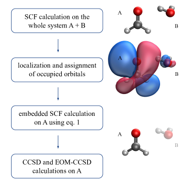
Figure 1: Flow of action in an embedded EOM-CCSD calculation.

Subsequently, the density matrix for the embedded fragment A is re-computed in a second self-consistent field calculation [54]. This is done using the modified Fock matrix

$$\widetilde{\mathbf{F}}^{\text{A-in-B}}[\boldsymbol{\gamma}^{\text{A}}] =(\mathbf{I}-\mathbf{S}\boldsymbol{\gamma}^{B})\,\mathbf{F}^{\text{A-in-B}}[\boldsymbol{\gamma}^{\text{A}}]\,(\mathbf{I}-\boldsymbol{\gamma}^{B}\mathbf{S})~{},$$ (1)

$$\mathbf{F}^{\text{A-in-B}}[\boldsymbol{\gamma}^{\text{A}}] =\mathbf{h}+\mathbf{g}[\boldsymbol{\gamma}^{\text{A}}]+\mathbf{v}_{\text{emb}}^{\text{A-in-B}}$$

by projecting out the occupied orbitals assigned to fragment B, and thereby enforcing orthonormality among all occupied orbitals. Here, h denotes the one-electron Hamiltonian, g the mean-field two-electron potential, and S the overlap matrix. The embedding potential is given as $\mathbf{v}_{\text{emb}}^{\text{A-in-B}}=\textbf{g}[\boldsymbol{\gamma}^{\text{A+B}}]-\textbf{g}[\boldsymbol{\gamma}^{\text{A}}]$. This approach is equivalent to the original formulation [54, 87] where the projector was chosen as $\mu\,\mathbf{S}\boldsymbol{\gamma}^{\text{B}}\mathbf{S}$ with $\mu$ as a large constant. The converged density matrix $\boldsymbol{\gamma}^{\text{A}}$ forms the basis for the subsequent EOM-CCSD treatment of subsystem A. No modifications of the CCSD and EOM-CCSD equations are necessary to this end.

To truncate the virtual orbital space, we employ concentric localization [68]: In this approach, the full virtual orbital space is projected on fragment A and an initial set of virtual orbitals is obtained from a singular value decomposition of the overlap between the full and the projected virtual space. The full virtual space can then be reconstructed in an iterative fashion by analyzing the coupling of the orbital spaces through the Fock operator giving tunable accuracy. In this work, the virtual space consists of the initial and one further set of orbitals unless indicated otherwise.

2.2 Dyson orbitals and natural transition orbitals

Similar to other quantum chemistry methods, it is also in the framework of projection-based embedding important to characterize changes in the wave function upon excitation, ionization, or electron attachment. Two quantities that are useful in this context are Dyson orbitals [27, 28, 29, 30, 31, 32, 33] and natural transition orbitals (NTOs) [34, 35, 36, 37, 38, 33]. Within projection-based embedded EOM-CC, we can define and evaluate these quantities in analogy to regular EOM-CC. Dyson orbitals $\phi_{d}$ are given as

$$\phi_{d}(1)=\sqrt{n}\;\int\!\!\mathrm{d}1\,\mathrm{d}2\dots\mathrm{d}n\;\;\Psi_{n}^{*}(1,2,\dots,n)\;\;\Psi_{n-1}(2,\dots,n)$$ (2)

and can be viewed as generalized transition density matrices between a pair of states with $n$ and $n-1$ electrons, respectively. EOM-CC Dyson orbitals thus characterize ionization or electron attachment based on the correlated many-electron wave functions taking part in the transition. Notably, Eq. (2) is not limited to the ground state but can be applied to ionization or attachment involving excited states as well [29]. Because of the asymmetry of the similarity transformed Hamiltonian in EOM-CC theory, pairs of left and right Dyson orbitals exist but they usually differ only marginally.

NTOs arise from a singular value decomposition of the transition density matrix $\boldsymbol{\gamma}^{IF}$ for a pair of states $\Psi_{I}$ and $\Psi_{F}$,

$$\boldsymbol{\gamma}^{IF}(1,1^{\prime}) =n\int\!\!\mathrm{d}1\,\mathrm{d}2\dots\Psi_{I}^{*}(1,2,\dots,n)\;\Psi_{F}(1^{\prime},2,\dots,n)$$ (3)

$$=\sum_{K}\sigma_{K}\psi^{p}_{K}(1)\psi^{h}_{K}(1^{\prime})~{},$$

$$\psi_{K}^{p}(1) =\sum_{q}\,V_{qK}\,\phi_{q}(1)~{},\quad\psi_{K}^{h}(1)=\sum_{q}\,U_{qK}\,\phi_{q}(1)~{}.$$

Here, $\psi_{K}^{p}$ and $\psi_{K}^{h}$ denote particle and hole NTOs, respectively, while $\phi_{q}$ is a generic molecular orbital. The singular values $\sigma_{K}$ provide a measure of the contribution of a particular NTO pair to the overall transition and usually only very few of them are large. In EOM-CC theory, pairs of NTOs exist because $\boldsymbol{\gamma}^{IF}\neq\boldsymbol{\gamma}^{FI}$ but the differences are again marginal.

2.3 Electronic resonances

Electronic resonances are states that are metastable towards electron loss [49, 88]. Such states cannot be tackled with conventional quantum chemistry methods because their wave functions are not square integrable in Hermitian quantum mechanics. Within non-Hermitian quantum mechanics,[88] however, the energy of a resonance can be defined as

$$E=E_{R}-i\,\Gamma/2~{},$$ (4)

where the real part is the position of the resonance and the imaginary part the half-width, which is related to the state’s lifetime, $\tau=1/\Gamma$. Among the different non-Hermitian approaches that were introduced for the treatment of electronic resonances [49, 88], we use here the complex absorbing potential (CAP) approach [43]. Here, the Hamiltonian is augmented by an artificial potential $W$ that absorbs the diverging tail of the resonance wave function. The energy eigenvalues of the CAP Hamiltonian $H(\eta)=H-i\,\eta\,W$ will depend on the shape of the potential $W$ and on the CAP strength $\eta$. Its optimal value $\eta_{opt}$ is found by computing energies for a range of $\eta$ values and minimizing the quantity $|\eta\,dE/d\eta|$ [43]. In this work, shifted quadratic CAPs are used and the CAP-free region is determined either based on Voronoi cells [89] or takes the form of a box.

Different variants of CAP-EOM-CC methods can be distinguished depending on whether the CAP is included already in the Hartree-Fock (HF) calculation, or at the CCSD level, or only at the EOM-CCSD level.[49] In this work, the third approach is employed, that is, the CAP is added only at the EOM-CCSD level. In addition, the CAP is projected on the virtual orbital space [90]. Although this approach is less consistent than the first one from a formal standpoint [49], it offers an advantage in the context of quantum embedding: since the HF reference wave function is real-valued, the embedding procedure need not be adapted to non-Hermitian quantum chemistry. Moreover, the computational cost is considerably lower because only a single CAP-free CCSD calculation (scaling as $\mathcal{O}(o^{2}\,v^{4})$) is needed for the reference state, whereas the EOM-CCSD part, which scales as $\mathcal{O}(o\,v^{4})$ for electron attachment, needs to be repeated for different values of $\eta$. It can also be argued that the CAP represents nothing but a perturbation for the bound reference state that should be avoided.

2.4 Technical details

In all computations except those for charge transfer states, the environment B consists of a varying number (1–5) of water molecules, whereas we take different small molecules as fragment A: formaldehyde (CH₂O), methanol (CH₃OH), ethylene (C₂H₄), methylene (CH₂), fluoromethylene (HCF), silylene (SiH₂), dinitrogen (N₂), and carbon monoxide (CO). These systems are small enough to be treated as a whole by EOM-CCSD and the comparison between full and embedded EOM-CCSD is the centerpiece of our work. Furthermore, we report transition energies obtained with computationally cheaper alternatives: Ionization and electron-attachment energies are calculated with $\Delta$DFT using the maximum overlap method (MOM) [91] and for excited states TD-DFT calculations are carried out within the Tamm-Dancoff approximation (TDA/TD-DFT)[92, 93]. As concerns charge transfer, we investigate two systems: HCl (A) embedded in 5 H₂O (B), where charge transfer takes place in the HCl molecule, and the donor-acceptor complex NH${}_{3}\cdots$F₂ where we take the donating NH₃ molecule as fragment A and the accepting F₂ molecule as fragment B.

The structures of the systems consisting of two molecules, that is, A + H₂O and the CO₂ and N₂ dimers, are optimized with RI-MP2/cc-pVTZ unless stated otherwise. Clusters composed of four and six molecules, that is, fragment A + 3 or 5 H₂O, are generated starting from the optimized structure of A. All geometries can be found in the Supporting Information (SI). The following density functionals are used as low-level method in the embedded EOM-CCSD calculations and also for standalone $\Delta$DFT and TD-DFT calculations: PBE [94] and BLYP [95, 96] (generalized gradient approximation (GGA) functionals), PBE0 [97] (hybrid GGA functional), as well as CAM-B3LYP [98], $\omega$B97X-D [99], and LC-$\omega$PBE08 [100] (range-separated hybrid functionals). The subsequent CCSD and EOM-CCSD calculations are always based on a HF reference wave function for the embedded fragment A and the core orbitals of A are always included in the correlation treatment except for core ionization energies. Here, the frozen-core/core-valence-separation (fc-CVS) scheme [101, 102, 103] is employed for the clusters comprising more than one water molecule because convergence of the EOM-CCSD equations is not achieved otherwise.

The correlation-consistent basis set aug-cc-pVTZ [104] is employed for most systems. For temporary anions and Rydberg excited states, respectively, this basis is augmented with 3 or 2 additional $s$ and $p$ shells of diffuse functions. These extra shells are generated in an even-tempered manner, i.e., by recursively dividing the exponent of the most diffuse $s$ and $p$ shell by a factor of 2. All calculations were performed with a slightly modified version of the Q-Chem electronic structure package [105, 106] using the implementation of projection-based embedding included in the 5.3 release of the program [87]. Results of embedded EOM-EE-CCSD calculations were verified against results presented in Ref. 78.

3 Results for bound states

3.1 Performance of embedded EOM-CCSD at different distances between the fragments

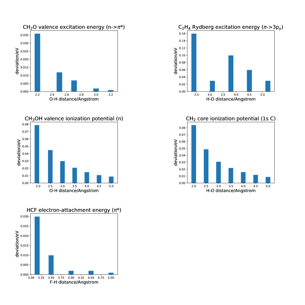
Figure 2: Absolute value of the deviation between transition energies computed with EOM-CCSD embedded in PBE0 and with full EOM-CCSD. All systems are composed of a molecule in which the excitation takes place and a single water molecule that acts as environment. The deviation is shown as a function of the distance between the two fragments.

Figure 2 presents deviations of embedded EOM-CCSD from full EOM-CCSD as a function of the intermolecular distance between the fragments. Representative examples of a valence excitation, a Rydberg excitation, a valence ionization, a core ionization, and an electron attachment are shown; the lower-level fragment always consists of a single H₂O molecule. In all these calculations, the full virtual orbital space is taken into account in the embedded EOM-CCSD calculation.

Figure 2 illustrates that the deviations between embedded and full EOM-CCSD decrease with the intermolecular distance and stay below 0.1 eV even at the shortest distance. This holds true for every type of transition that we examined with the notable exception of Rydberg excitations. In this case, not only is the trend not observed anymore, but also the absolute deviations are larger and the performance depends on the orbital to which the electron is excited. This might be tied to the spatial extension of Rydberg states, which are perturbed more strongly by the presence of the water molecule also at a larger distance, and are more sensitive to the relative orientation. We note that Bennie et al. observed as well that the deviation between embedded and full EOM-CCSD decreases with growing intermolecular distance for valence excited states [78].

The same trend is observed in larger clusters where the lower-level fragment comprises 5 H₂O molecules. In Tables 3.3 and 3.3, deviations between embedded and full EOM-CCSD are shown for a valence excitation of CH₂ and a valence ionization of C₂H₄, respectively. Two configurations near and far are compared: In the first cluster, the distances between all water molecules and the excited or ionized molecule lie around 2–3 $\mathrm{\SIUnitSymbolAngstrom}$, in the other cluster they are of the order of 5 $\mathrm{\SIUnitSymbolAngstrom}$. The errors differ heavily between the two clusters: For the configuration far, they are smaller by a factor of up to 100 as compared to the configuration near. We note that the manual inclusion of additional occupied orbitals in the high-level fragment can improve the performance of embedded EOM-CCSD at short distances [78], this is however not explored further here.

3.2 Influence of the size of the environment region

Tables 3.3–3.3 report deviations between embedded and full EOM-CCSD for clusters in which the environment consists of three or five water molecules. The results are grouped by type of state, negative deviations correspond to a transition energy lower than that of full EOM-CCSD. For these clusters, the distances between the water molecules and the embedded fragment vary among the configurations, but they usually lie in the lower half of the distances presented in Figure 2 at which correlation effects are more important and the performance of the embedded method is less good.

As we can see from the comparison of error values reported in Figure 2 and Tables 3.3–3.3, for the same type of transition and the same molecule, the error due to embedding generally increases with the amount of water molecules in the environment. The performance differs considerably among the individual molecules and also depends on the density functional used to treat the environment, but the deviations between embedded and full EOM-CCSD for the clusters with three or five water molecules can exceed those for the two-molecule clusters by a factor of 10 and more.

On the other hand, the configuration of the larger clusters has a relatively small effect on the deviation of the embedded energies, provided that the distances between the water molecules and the high-level fragment lie in the same range. Electron attachment (see Table 3.3) shows the highest sensitivity: Configurations 1, 2 and 4 of HCF, where embedded EOM-EA-CCSD performs particularly poorly, have in common a single water molecule positioned such that the electron density of the oxygen lone pair faces the halocarbene.

3.3 Performance for different types of target states

In this section, we analyze the performance of projection-based embedded EOM-CCSD with respect to the type of transition. This is again done based on the data presented in Tables 3.3–3.3.

Valence excitation energies calculated with full EOM-EE-CCSD, embedded EOM-EE-CCSD, and TD-DFT using the aug-cc-pVTZ basis set. Embedded EOM-EE-CCSD and TD-DFT results (last three columns) are reported as deviations from full EOM-EE-CCSD. All values in eV. System Transition Configuration full EOM-CCSD EOM-CCSD in PBE EOM-CCSD in CAM-B3LYP TDA/ TD-CAM-B3LYP CH₂O + 5H₂O n$\rightarrow$ $\pi$* 1 4.08 0.04 0.05 -0.06 2 4.02 0.001 0.01 -0.05 3 3.92 -0.008 0.004 -0.06 4 4.00 0.02 0.02 -0.05 5 3.94 0.008 0.01 -0.06 CH₃OH + 5H₂O n$\rightarrow$$\sigma$* 7.04 -0.54 -0.07 -0.64 HCF + 5H₂O $\pi$*$\rightarrow$$\pi$* 3.14 0.36 0.20 0.40 CH₂ + 5H₂O $\sigma$ $\rightarrow$ $\pi^{*}$ near 1.70 0.29 0.27 -0.07 far 1.66 0.002 0.004 -0.07

Valence excitations. As we can see from Table 3.3, excitation energies obtained with EOM-EE-CCSD embedded in PBE and CAM-B3LYP vary appreciably among the test cases. The two density functionals produce similar results in general, but the excitation energy can differ by up to 0.47 eV (CH₃OH + 5H₂O). Also, the errors of embedded EOM-EE-CCSD are comparable to the ones obtained with TD-CAM-B3LYP in most cases. We add that Bennie et al. presented a comparison to different density functionals as well and found that time-dependent PBE, PBE0, M06-2X, and HF perform significantly worse than embedded EOM-EE-CCSD in predicting the excitation energy of microsolvated formaldehyde and acroleine [78]. An exception is found among our results for CH₃OH, where EOM-CCSD embedded in CAM-B3LYP performs very well, whereas TD-CAM-B3LYP struggles to reproduce the full EOM-CCSD energy. This might be explained by the partial Rydberg character (3$s$) of this excited state [107] whose proper representation is difficult with TD-DFT.

Rydberg excitation energies calculated with full EOM-EE-CCSD, embedded EOM-EE-CCSD, and TD-DFT using the aug-cc-pVTZ+2s2p basis set. Embedded EOM-EE-CCSD and TD-DFT results (last three columns) are reported as deviations from full EOM-EE-CCSD. All values in eV. System Transition^a full EOM-CCSD EOM-CCSD in PBE EOM-CCSD in CAM-B3LYP TDA/ TD-CAM-B3LYP CH₂O + 3H₂O n$\rightarrow$3s 7.69 -0.17 0.05 -0.33 n$\rightarrow$3p_z 8.42 -0.19 0.01 -0.27 n$\rightarrow$3p_y 8.70 -0.36 0.03 -0.39 n$\rightarrow$3p_x 8.82 -0.13 0.05 -0.43 CH₃OH + 3H₂O n$\rightarrow$3p$\sigma$ 8.37 -0.27 -0.01 -0.60 n$\rightarrow$3p$\pi$ 8.75 -0.48 -0.03 -0.68 n$\rightarrow$3p$\sigma^{\prime}$ 8.85 -0.52 -0.08 -0.81 C₂H₄ + 3H₂O $\pi\rightarrow$3s 7.06 -0.21 0.09 -0.65 $\pi\rightarrow$3p_y 7.74 -0.15 0.04 -0.94 $\pi\rightarrow$3p_z 7.76 -0.08 0.11 -0.74 $\pi\rightarrow$3p_x 7.92 -0.02 0.12 -0.80 ^aAssignment follows Ref. 108 for CH₂O, Ref. 107 for CH₃OH and Ref. 109 for C₂H₄.

Rydberg excitations. Due to the incorrect asymptotic behaviour of local exchange-correlation functionals, lower-rung TD-DFT methods usually offer only a poor description of Rydberg excited states [110]. The performance improves when range-separated functionals are employed [111]. However, in Table 3.3 we can see than TD-CAM-B3LYP still deviates by 0.3–1.0 eV from full EOM-EE-CCSD. This is in contrast to EOM-EE-CCSD embedded in CAM-B3LYP, where deviations do not exceed 0.12 eV. In contrast to valence excitations, embedded EOM-CCSD thus represents a clear improvement over TD-CAM-B3LYP for Rydberg excitations. As observed for valence excited states as well, the choice of the low-level method has an impact on the results of embedded EOM-EE-CCSD: CAM-B3LYP produces significantly smaller deviations than PBE. This can be ascribed to the long-range HF exchange included in the former density functional and mimics the performance of the corresponding TD-DFT methods.

Excitation energies of charge transfer states calculated with full and embedded EOM-EE-CCSD/aug-cc-pVTZ and TD-DFT. All values in eV. System Transition full EOM- CCSD EOM- CCSD in PBE EOM- CCSD in BLYP EOM-CCSD in CAM- B3LYP TDA/ TD- PBE TDA/ TD- BLYP TDA/ TD-CAM- B3LYP HCl + 5H₂O $n\rightarrow\sigma$* 8.19 8.00 8.15 8.18 6.92 6.80 7.80 NH₃$\cdots$F₂ $n\rightarrow\sigma$* 4.49 3.12^a 5.27^a 6.51^a 0.31 0.28 4.87 ^aVirtual orbital space is not truncated.

Charge transfer states. Our results for intra- and intermolecular charge transfer are reported in Table 3.3. Embedded EOM-EE-CCSD describes the intramolecular process that occurs in HCl + 5H₂O with good accuracy; the excitation energy deviates only by 0.01 eV from full EOM-CCSD when CAM-B3LYP is used as low-level method. Although embedded EOM-EE-CCSD is more accurate than TD-DFT also with PBE and BLYP as low-level method, the dependence of the results on the density functional is not eliminated. PBE yields the largest error, while BLYP gives intermediate results that are slightly improved by error cancellation when the virtual orbital space is truncated. These results can be related to the fact that local density functionals do not provide a good description of charge transfer.[110]

As a test case for intermolecular transfer, we investigate the NH${}_{3}\cdots$F₂ complex that was used as a test case for the M06-HF density functional [112]. The same geometry is used here. The complex is divided such that the donating fragment (NH₃) is treated at the EOM-CCSD level, whereas the accepting one (F₂) constitutes the environment and is treated at the DFT level. We do not truncate the virtual orbital space in the embedded EOM-CCSD calculations so that it remains identical to that employed in the full EOM-CCSD calculations. However, even though the virtual orbital space is the same, embedded EOM-EE-CCSD does not perform well, the errors with respect to full EOM-EE-CCSD amount to up to 2 eV. It is also remarkable that embedding in CAM-B3LYP produces the worst results, while the lower-rung functionals BLYP and PBE lead to better results. Within TD-DFT, however, CAM-B3LYP provides an accurate description, whereas the GGA functionals are completely incapable of describing the charge transfer. We conclude that embedded EOM-CCSD provides a reliable description of charge transfer only if both the donor and the acceptor are part of the high-level fragment.

Valence ionization energies calculated with full EOM-IP-CCSD, embedded EOM-IP-CCSD, and $\Delta$DFT using the aug-cc-pVTZ basis set. Embedded EOM-IP-CCSD and $\Delta$DFT results (last four columns) are reported as deviations from full EOM-IP-CCSD. All values in eV. System Transition Configuration full EOM-CCSD EOM-CCSD in PBE EOM-CCSD in CAM-B3LYP $\Delta$CAM- B3LYP $\Delta$PBE CH₂O + 5H₂O $\pi$*$\rightarrow$$\infty$ 1 11.20 0.22 0.23 -0.24 -0.15 2 11.19 0.10 0.12 -0.15 -0.22 3 11.16 0.10 0.12 -0.20 -0.18 4 11.70 0.09 0.14 -0.45 0.66 5 11.12 0.14 0.15 -0.12 -0.15 HCF + 5H₂O n$\rightarrow$$\infty$ 10.16 0.37 0.56 -0.32 –^a CH₃OH + 5H₂O n$\rightarrow$$\infty$ 10.47 0.29 0.30 0.17 3.77 C₂H₄ + 5H₂O $\pi$$\rightarrow$$\infty$ near 8.98 0.64 0.64 0.23 -0.26 far 10.94 0.02 0.03 -0.10 -0.10 ^aPBE calculation of the ionized state does not converge.

Valence ionizations. As apparent from the comparison of Tables 3.3 and 3.3, the deviations between embedded and full EOM-CCSD are somewhat larger for the IP variant than for the EE variant. Similar to valence excitations, the dependence on the density functional used for the description of the environment is weak but significant differences are obtained in some cases. Among the cases we considered, the largest difference of ca. 0.2 eV occurs for HCF+5 H₂O. Remarkably, embedding in the lower-rung functional PBE produces better results for this case than embedding in CAM-B3LYP. By contrast, $\Delta$CAM-B3LYP is clearly superior to $\Delta$PBE and performs similar to embedded EOM-IP-CCSD. This implies that embedded EOM-IP-CCSD does not always represent an improvement over $\Delta$CAM-B3LYP if one is interested only in the ionization energies. However, a distinct advantage of all EOM-CC methods is that the wave functions for the ground and target state are biorthogonal so that transition properties can be readily evaluated. This is not the case in $\Delta$DFT approaches where the evaluation of further quantities besides the transition energy is not straightforward.

Core ionization energies calculated with full EOM-IP-CCSD, embedded EOM-IP-CCSD, and $\Delta$DFT using the aug-cc-pVTZ basis set. Embedded EOM-IP-CCSD and $\Delta$DFT results (last three columns) are reported as deviations from full EOM-IP-CCSD. Frozen core-CVS scheme is employed for full and embedded EOM-IP-CCSD calculations. All values in eV. System Transition Configuration full EOM-CCSD EOM-CCSD in PBE EOM-CCSD in CAM-B3LYP $\Delta$CAM- B3LYP CH₂O + 5H₂O 1s(C)$\rightarrow$$\infty$ 1 295.24 0.10 0.10 -0.33 2 295.27 0.05 0.06 -0.30 3 295.25 0.05 0.06 -0.31 4 295.79 0.02 0.06 -0.32 CH₂O + 5H₂O 1s(O)$\rightarrow$$\infty$ 1 540.98 0.11 0.12 -1.39 2 540.95 0.04 0.06 -1.40 3 540.95 0.05 0.06 -1.40 4 541.48 0.01 0.06 -1.46 HCF + 5H₂O 1s(C)$\rightarrow$$\infty$ 296.26 0.16 0.37 5.06 CH₂ + 5H₂O 1s(C)$\rightarrow$$\infty$ 293.06 0.20 0.28 -0.92

Core ionizations. Table 3.3 illustrates that embedded EOM-IP-CCSD performs on average somewhat better for core ionization than for valence ionization. The performance depends again only weakly on the low-level method used to describe the environment. Embedded EOM-IP-CCSD is significantly more accurate than $\Delta$DFT for core ionization, which is in contrast to what we saw for valence ionizations. However, is it necessary to consider here that the reference values (full fc-CVS-EOM-CCSD) are obtained with the CVS scheme [103] and the $\Delta$DFT values without. For some cases with an environment consisting of a single H₂O molecule, we found that fc-CVS-EOM-CCSD deviates from EOM-CCSD by up to 0.5 eV and the relatively large $\Delta$DFT errors in Table 3.3 might be partly a consequence of using fc-CVS-EOM-CCSD as reference.

A systematic investigation of this effect was, however, not possible for technical reasons: Since core-ionized states are unstable towards Auger decay, they are embedded in the continuum [49]. This leads to convergence problems for the EOM-CCSD equations of core ionized states [113]; for the larger clusters with an environment of 5 H₂O molecules, we were unable to achieve convergence. With the CVS scheme,[101] the continuum is projected out from the excitation space and the core-ionized states can be obtained without problems. We add here that CVS-EOM-CCSD and regular EOM-CCSD both represent approximations because they ignore the resonance character of core-ionized states. However, whereas CVS is a well-defined approximation, the approximation in regular EOM-CCSD is less obvious and, in fact, uncontrolled because the results depend on how the continuum is discretized by the finite basis set.

Electron attachment energies calculated with full and embedded EOM-EA-CCSD/aug-cc-pVTZ and with $\Delta$DFT. Column headings “full” and “trunc.” refer to calculations using the full and a truncated virtual orbital space, respectively. All values in eV. System Transition Configuration full EOM- CCSD EOM-CCSD in PBE EOM-CCSD in CAM-B3LYP EOM-CCSD in HF $\Delta$CAM- B3LYP full trunc. full trunc. full HCF + 5H₂O $\infty$$\rightarrow$$\pi$* 1 0.34^a -0.60 -0.21 0.06^a 0.40^a 0.56^a -0.21 2 0.24^a -1.03 -0.25 -0.19 0.23^a 0.33^a -0.30 3 0.27^a -0.18 -0.29 -0.15 0.34^a 0.47^a -0.93 4 0.13^a -0.96 -0.46 -0.50 0.21^a 0.39^a -0.12 5 -0.07 -1.42 -1.06 -0.41 -0.01 0.16 -1.33 CH₂ + 5H₂O $\infty$$\rightarrow$$\pi$ 0.36^a -0.64 0.001^a 0.04^a 0.56^a 0.58^a 0.03^a SiH₂ + 5H₂O $\infty$$\rightarrow$$\pi$ -0.28 -0.57 -0.36 -0.25 -0.17 0.05^a 0.30^{a a}Positive electron-attachment energies correspond to unbound states. The physical significance of these discretized continuum states is limited.

Electron attachment. Table 3.3 presents our results for electron attachment energies calculated with embedded EOM-EA-CCSD. It can be seen that, in general, the EA variant performs significantly worse than the EE and IP variants. In fact, when tackling electron attachment, high accuracy is always needed because attachment energies are typically smaller than excitation or ionization energies. Thus, even a small error can have strong repercussions on the results. Table 3.3 shows that several states that are unbound according to full EOM-EA-CCSD become artificially bound with embedded EOM-EA-CCSD.

This problem is already present at the self-consistent field level: We observe in many embedding calculations virtual orbitals with negative energies emerging that are not present in regular self-consistent field calculations. The inclusion of very diffuse functions in the basis set, as is required for Rydberg states and resonances, appears to trigger the emergence of these orbitals. They cannot be easily recognized by their shape or in some other way but electron attachment to them and excitations into them are not physically meaningful because no corresponding orbitals exist in the self-consistent field calculations for the full system. In our EOM-EE-CCSD calculations for Rydberg states, excitations involving these orbitals were easy to discern by the unphysical shape of the corresponding NTOs but this may not be the case if the environment is more complex and consists not only of water molecules.

In general, electron attachment energies depend much more strongly on the density functional used to describe the environment than other transition energies. One might expect that long-range corrected functionals improve the description [114, 115] but we found that the problems largely persist with CAM-B3LYP. Also here, virtual orbitals with an artificial negative energy are obtained. A significant improvement is obtained when the low-level fragment is described at the HF level, but these calculations suffer in a few cases from the opposite problem, that is, a state that is bound according to full EOM-EA-CCSD becomes unbound.

Table 3.3 also shows that the results of embedded EOM-EA-CCSD calculations depend significantly on the truncation of the virtual orbital space. This is in contrast to all other types of states investigated in this work and will be discussed in more detail in Sec. 3.4. Contrary to the intuition, more accurate attachment energies are in most cases obtained with a truncated virtual orbital space. This is probably due to error cancellation and we conclude that care should be applied when using embedded EOM-EA-CCSD.

3.4 Truncation of the virtual orbital space

In order to carry out embedded EOM-CCSD calculations with large environments, it is critical to truncate the virtual orbital space. As outlined in Section 2, we use here concentric localization [68] to this end. To test the validity of this procedure for different types of target states, we compare energies obtained with truncated and untruncated virtual orbital spaces. Our numerical results can be found in the SI and are discussed in the following.

We observe that the impact of the truncation is smallest for valence and core ionization energies. Here, the errors caused by concentric localization are consistently smaller than 10^-5 a.u. This is not a surprise because the virtual orbitals are not needed for a zeroth-order description of ionized states and enter only at higher orders. Valence excitation energies are not heavily affected by the truncation either; we observe a maximum deviation of 0.01 eV among our test cases for the transition in HCF.

The excitation energy of CH₃OH is an exception as it exhibits truncation errors of 0.1 eV and 0.05 eV for EOM-CCSD in PBE and CAM-B3LYP, respectively. We relate this to the partial Rydberg character of this state because we observe in general larger truncation errors when the electron is excited to more spatially extended orbitals. While the performance of concentric localization is overall still satisfactory for Rydberg states with deviations of 0.01–0.02 eV in many cases, there are some cases with significantly larger deviations. For the 3$p_{y}$ state of formaldehyde, concentric localization leads to a difference of 0.08 eV in the excitation energy. Moreover, there are no clear trends: Due to different orientations and a varying degree of delocalization over the environment molecules, the truncation process can yield different results for each state in a Rydberg series.

We also notice that excitation energies are less sensitive towards truncation of the virtual orbital space when CAM-B3LYP is employed as low-level method for the environment as compared to PBE. The same trend is observed for the intramolecular charge-transfer state in HCl: the difference in energies with and without the application of concentric virtual localization is 0.05, 0.04, and 0.01 eV for embedding in PBE, BLYP and CAM-B3LYP, respectively.

Most sensitive towards truncation of the virtual orbital space are electron attachment energies. Here, the error due to concentric localization is of the same order of magnitude as the one due to embedding itself and the results do not change significantly until the full virtual orbital space is recovered. This may be related to the fact that already a zeroth-order description of electron-attached states involves the virtual orbitals. As alluded to in the previous section (see Table 3.3), concentric localization improves the agreement with full EOM-EA-CCSD in many cases, likely due to error cancellation. However, the performance is still inferior to the other embedded EOM-CCSD variants and further investigations are needed to exploit the cancellation of errors in a useful way.

As a final remark, we note that EOM-CCSD calculations with a truncated virtual space appear to be more likely to converge to a solution that is dominated by an excitation involving an artificial virtual orbital than calculations with the full virtual space. However, concentric localization is not the origin of this problem as virtual orbitals with artificial negative energies are also present without truncation.

3.5 Natural transition orbitals and Dyson orbitals

Figure 3: Upper row: Particle NTOs for excitations to the 3s, 3p_x, 3p_y, and 3p_z Rydberg orbitals of C₂H₄ computed with EOM-EE-CCSD/aug-cc-pVTZ+2s2p. Lower row: Corresponding particle NTOs for C₂H₄ + H₂O computed with EOM-EE-CCSD embedded in PBE0/aug-cc-pVTZ+2s2p. All NTOs have been plotted at an isovalue of 0.001.

Figure 3 shows the particle NTOs for several Rydberg states of isolated ethylene and of ethylene in the presence of a water molecule located nearby in the molecular plane ($yz$-plane). It can be seen that the environment participates in the transition to a varying degree: none of the NTOs is unaffected by the presence of the water molecule but the NTOs of the 3p_y and the 3p_z state are more significantly distorted than those of the 3s state and the 3p_x state.

To quantify the similarity between NTOs from embedded and full EOM-EE-CCSD calculations, we compare in Table 3.5 the largest singular values of the transition density matrices. Overall, excellent agreement between the two approaches is observed. Furthermore, we notice that when the difference in the transition energy increases, so does the difference between the singular values. The largest deviations are observed for the 3p_y and the 3p_z state in agreement with Fig. 3.

Energies $E$ and largest singular values $\sigma$ of the transition density matrix computed with full EOM-EE-CCSD for the Rydberg series of C₂H₄+H₂O and deviations $\Delta E$ and $\Delta\sigma$ for EOM-EE-CCSD embedded in PBE0. All values are computed using the aug-cc-pVTZ+2s2p basis set. Full EOM-EE-CCSD EOM-EE-CCSD in PBE0 Transition $E$ / eV $\Delta E$ / eV $\sigma$ / a.u. $\Delta\sigma$ / a.u. $\pi\rightarrow$3s 7.15 0.07 0.87 0.006 $\pi\rightarrow$3p_y 7.72 0.16 0.86 0.013 $\pi\rightarrow$3p_x 7.84 0.11 0.86 0.010 $\pi\rightarrow$3p_z 8.10 0.01 0.87 0.004

As a further example, we present Dyson orbitals for valence and core ionization of CH₂O and CH₂O + H₂O in Figure 4. The comparison to Figure 3 shows that Dyson orbitals are, in general, less affected by the environment than particle NTOs. Only for the Dyson orbital that describes valence ionization of the ground state, some participation of the environment can be seen in the plot. On the contrary, no difference is visible for the Dyson orbitals that describe valence ionization of the first excited state and core ionization of the ground state. Consistent with this, the ionization energy corresponding to the first Dyson orbital changes by almost 0.4 eV in the presence of the H₂O molecule while the other two ionization energies change by only 0.26 eV and 0.22 eV.

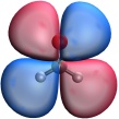
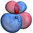
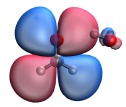
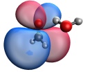
Figure 4: Upper row: Dyson orbitals for valence ionization of the ground state, valence ionization of the lowest excited state, and 1s(C) core ionization of CH₂O computed with EOM-IP-CCSD/aug-cc-pVTZ. Lower row: Corresponding Dyson orbitals for CH₂O + H₂O computed with EOM-IP-CCSD embedded in PBE0/aug-cc-pVTZ. The frozen-core-CVS scheme has been employed for the core-ionized state. Dyson orbitals describing valence ionization have been plotted at an isovalue of 0.005, those describing core ionization at an isovalue of 0.007.

4 Results for electronic resonances

4.1 Localized electron attachment

We test the performance of projection-based embedding combined with CAP-EOM-EA-CCSD first on the temporary anions CO^- and CH₂O^- solvated by one water molecule. In these systems, the extra electron occupies the $\pi$* orbital of the C–O bond of CO or CH₂O, that is, the excess electron density is localized.

From the data in Table 4.1, we observe that CAP-EOM-EA-CCSD embedded in PBE reproduces full CAP-EOM-EA-CCSD results with high accuracy ($10^{-2}$ eV) for positions and widths. The results are also largely independent of the CAP shape. This good agreement of energies and decay widths obtained with embedding justifies in retrospect our approach to apply the CAP only to the EOM-CCSD part. However, the deviation between embedded CAP-EOM-EA-CCSD and full EOM-EA-CCSD increases when the distance between the transient anion and water decreases. This is in line with our results obtained for bound anions microsolvated by one molecule of water.

Resonance positions and widths of CH₂O^- and CO^- microsolvated by one H₂O molecule computed with embedded and full CAP-EOM-EA-CCSD/aug-cc-pVTZ+3s3p at different intermolecular distances. Box CAP onsets and optimal $\eta$ values are reported in the SI. All values in eV. System Intermolecular CAP-EOM-CCSD CAP-EOM-CCSD in PBE Distance/$\mathrm{\SIUnitSymbolAngstrom}$ $E_{R}$ $\Gamma$ $E_{R}$ $\Gamma$ box CAP CH₂O^- 1.07 0.38 CH₂O^- + H₂O 2.2 0.88 0.20 0.91 0.22 CO^- 2.07 0.60 CO^- + H₂O 2.0 1.68 0.47 1.72 0.55 CO^- + H₂O 2.5 1.82 0.56 1.85 0.58 CO^- + H₂O 3.0 1.91 0.55 1.92 0.55 CO^- + H₂O 4.0 1.99 0.53 1.99 0.54 Voronoi CAP (cutoff: 4 $\mathrm{\SIUnitSymbolAngstrom}$) CO^- + H₂O 2.0 1.67 0.56 1.72 0.52 CO^- + H₂O 2.5 1.82 0.56 1.83 0.55 CO^- + H₂O 3.0 1.90 0.57 1.90 0.60 CO^- + H₂O 4.0 1.99 0.60 1.98 0.62

4.2 Delocalized electron attachment

When the excess electron density is delocalized over the environment, embedded CAP-EOM-EA-CCSD does not perform equally well. Here, we report results for the temporary anions (CO)${}_{2}^{-}$ and (N₂)${}_{2}^{-}$. Four resonance states can be identified in these dimers; they arise from the combination of the $\pi$* orbitals in CO or N₂, respectively. We note that (CO)${}_{2}^{-}$ has been studied before in Ref. 116, here we use the same geometry.

To test the applicability of projection-based embedding, only one of the monomers is included in the CAP-EOM-EA-CCSD calculation, while the other one constitutes the environment. We do not truncate the virtual orbital space in these calculations, so the virtual orbitals of both monomers take part in the CAP-EOM-CCSD treatment. The density functionals PBE and CAM-B3LYP are assessed for both dimers, for (CO)${}_{2}^{-}$ we investigate in addition HF, $\omega$B97X-D, and LC-$\omega$PBE08.

In none of these cases are the results satisfactory. With PBE as low-level method, artificial bound states appear, i.e., states with a negative attachment energy, thus making it inappropriate for the description of such systems. This is reminiscent of the problems of EOM-EA-CCSD embedded in PBE that we observed for bound anions (see Sec. 3). The problem with artificial bound states is not present with the other density functionals or HF theory, which confirms our previous finding that longe-range corrected functionals improve the performance of embedded EOM-EA-CCSD. However, large deviations from full CAP-EOM-EA-CCSD still persist as demonstrated by Table 4.2. Therefore, we conclude that for a correct description of temporary anions with a delocalized excess electron density, all parts of the system have to be treated on an equal footing.

Resonance positions and widths of (CO)${}_{2}^{-}$ and (N₂)${}_{2}^{-}$ computed with embedded and full CAP-EOM-EA-CCSD/aug-cc-pVTZ+3s3p. Box CAP onsets and optimal $\eta$ values are reported in the SI. All values in eV. CAP-EOM-CCSD CAP-EOM-CCSD CAP-EOM-CCSD CAP-EOM-CCSD CAP-EOM-CCSD in CAM-B3LYP in $\omega$B97X-D in LC-$\omega$PBE08 in HF State $E_{R}$ $\Gamma$ $E_{R}$ $\Gamma$ $E_{R}$ $\Gamma$ $E_{R}$ $\Gamma$ $E_{R}$ $\Gamma$ (CO)${}_{2}^{-}$ A_u 1.40 0.92 0.94 0.23 0.82 0.28 1.56 0.17 1.92 0.60 A_g 1.72 0.23 1.07 0.19 0.96 0.10 1.57 0.41 2.05 0.27 B_g 2.31 0.29 2.50 0.58 2.08 0.52 2.21 0.32 —^a —^a B_u 2.91 0.51 2.78 0.70 2.45 0.49 2.68 0.53 —^a —^a (N₂)${}_{2}^{-}$ 1A^′ 2.28 0.44 1.13 0.08 1A^′′ 2.32 0.61 1.25 0.15 2A^′′ 2.62 0.24 2.45 0.59 2A^′ 2.93 0.43 2.65 0.40 ^aThese resonances could not be observed.

5 Conclusions

We have investigated the performance of projection-based embedding by means of a comprehensive benchmark set of various types of electronic states. Different flavors of embedded EOM-CCSD were applied to microsolvated small organic molecules and the results were compared to full EOM-CCSD. We found that embedded EOM-CCSD, in general, works best if the distance between the high-level fragment and the environment is large; we also observed a mild systematic deterioration if the environment comprises five instead of one single water molecule.

Most interesting, however, is the comparison between different types of target states: in agreement with previous investigations [78, 80], we found that embedded EOM-CCSD in general works very well for valence excitations. Our investigations show that the same can also be said about valence and core ionizations, intramolecular charge transfer, as well as Rydberg excitations, although the use of range separated density functionals for the environment proves to be crucial for the latter. Moreover, all these types of transitions are fairly robust towards truncation of the virtual orbital space so that the investigation of more extended systems, where the environment is larger than in our current work, is straightforward. We note that TD-DFT and $\Delta$DFT are competitive alternatives for valence excitations and ionizations. The clearest improvement over a simple DFT approach is thus obtained for Rydberg excitations and core ionizations according to our results. A further important advantage of embedded EOM-CCSD over $\Delta$DFT approaches is the possibility to compute not only transition energies but also further quantities such as Dyson orbitals, which we have introduced in this work alongside natural transition orbitals.

In contrast to ionization and excitation, electron attachment proves to be more challenging to describe with embedded EOM-CCSD. The appearance of virtual orbitals with unphysical negative energy eigenvalues can in many cases not be avoided, the truncation of the virtual orbital space changes attachment energies significantly and, while some results benefit from error cancellation, the overall performance of the method is not satisfying. However, the extension from bound to temporary anions by means of complex absorbing potentials is straightforward and delivers good results for energies and decay widths as long as the excess electron density remains localized. Applications to temporary anions are, however, subject to the same limitation as those to bound anions: the virtual orbital space cannot be easily truncated. Some refinement of the embedding procedure thus appears to be essential to obtain a viable approach for electron attachment.

Associated content

The supporting information available for this work contains all molecular structures, relevant energies and technical parameters of the complex absorbing potentials calculations.

References

- [1] E. Alizadeh, T.M. Orlando and L. Sanche, Annu. Rev. Phys. Chem. 66, 379 (2015).
- [2] I.I. Fabrikant, S. Eden, N.J. Mason and J. Fedor, Adv. At. Mol. Opt. Phys. 66, 545 (2017).
- [3] M. Vacher, I.F. Galván, B.-W. Ding, S. Schramm, R. Berraud-Pache, et al. 118, 6927 (2018).
- [4] N.J. Hestand and F. C. Spano, Chem. Rev. 118, 7069 (2018).
- [5] D. Casanova, Chem. Rev. 118, 7164 (2018).
- [6] A.V. Marenich, J. Ho, M.L. Coote, C.J. Cramer, D.G. Truhlar, Phys. Chem. Chem. Phys. 16, 15068 (2014).
- [7] U. Aslam, V.G. Rao, S. Chavez, S. Linic, Nat. Catal. 1, 656 (2018).
- [8] A.I. Krylov, Rev. Comp. Chem. 30, 151 (2017).
- [9] H. Lischka, D. Nachtigallová, A.J.A. Aquino, P.G. Szalay, F. Plasser, F.B.C. Machado, and M. Barbatti, Chem. Rev. 118, 7293 (2018).
- [10] S. Ghosh, P. Verma, C.J. Cramer, L. Gagliardi, D.G. Truhlar, Chem Rev. 118 7249 (2018).
- [11] S.J.R. Lee, M. Welborn, F.R. Manby, and T.F. Miller, Acc. Chem. Res. 52, 1359 (2019).
- [12] R. Izsák, WIREs Comput. Mol. Sci. 10, e1445 (2020).
- [13] L.O. Jones, M.A. Mosquera, G.C. Schatz, and M.A. Ratner, J. Am. Chem. Soc. 142, 3281 (2020).
- [14] K. Emrich, Nucl. Phys. A 351, 379 (1981).
- [15] H. Sekino and R. J. Bartlett, Int. J. Quantum Chem. S18, 255 (1984).
- [16] J.F. Stanton and R.J. Bartlett, J. Chem. Phys. 98, 7029 (1993).
- [17] M. Nooijen, J.G. Snijders, Int. J. Quantum Chem. 48, 15 (1993).
- [18] J.F. Stanton and J. Gauss, J. Chem. Phys. 101, 8938 (1994).
- [19] M. Nooijen and R.J. Bartlett, J. Chem. Phys. 102, 3629 (1996).
- [20] A.I. Krylov, Annual Review of Physical Chemistry 59, 433 (2008).
- [21] K. Sneskov and O. Christiansen, WIREs Comput. Mol. Sci. 2, 566 (2012).
- [22] I. Shavitt and R.J. Bartlett, Many-Body Methods in Chemistry and Physics: MBPT and Coupled-Cluster Theory (Cambridge University Press, Cambridge, UK, 2009).
- [23] H.J. Monkhorst, Int. J. Quantum Chem. 12, 421 (1977)
- [24] D. Mukherjee and P.K. Mukherjee, Chem. Phys. 39, 325 (1979).
- [25] E. Dalgaard and H.J. Monkhorst, Phys. Rev. A 28, 1217 (1983).
- [26] H. Koch and P. Jórgensen, J. Chem. Phys. 93, 3333 (1990).
- [27] J. Linderberg and Y. Öhrn, Propagators in Quantum Chemistry (Academic, London, 1973).
- [28] L. S. Cederbaum and W. Domcke, Adv. Chem. Phys. 36, 205 (1977).
- [29] C. M. Oana and A. I. Krylov, J. Chem. Phys.127, 234106 (2007).
- [30] T.-C. Jagau and A. I. Krylov, J. Chem. Phys. 144, 054113 (2016).
- [31] M. L. Vidal, A. I. Krylov, and S. Coriani, Phys. Chem. Chem. Phys. 22, 3744 (2020).
- [32] J. V. Ortiz, J. Chem. Phys. 153, 070902 (2020).
- [33] A.I. Krylov, J. Chem. Phys. 153, 080901 (2020).
- [34] A. V. Luzanov, A. A. Sukhorukov, and V. E. Umanskii, Theor. Exp. Chem. 10, 354 (1976).
- [35] A.V. Luzanov and V.F. Pedash, Theor. Exp. Chem. 15, 338 (1979).
- [36] R.L. Martin, J. Chem. Phys. 118, 4775 (2003).
- [37] F. Plasser, M. Wormit, and A. Dreuw, J. Chem. Phys. 141, 024106 (2014).
- [38] S.A. Mewes, F. Plasser, A.I. Krylov, A. Dreuw, J. Chem. Theory Comput. 14, 710 (2018).
- [39] M. Kállay and J. Gauss, J. Chem. Phys. 121, 9257 (2004).
- [40] J. Aguilar and J.M. Combes, Commun. Math. Phys. 22, 269 (1971).
- [41] E. Balslev and J.M. Combes, Commun. Math. Phys. 22, 280 (1971).
- [42] C.W. McCurdy and T. Rescigno, Phys. Rev. Lett. 41, 1364 (1978).
- [43] U.V. Riss and H.-D. Meyer, J. Phys. B 26, 4503 (1993).
- [44] A. Ghosh, N. Vaval, and S. Pal, J. Chem. Phys. 136, 234110 (2012).
- [45] K.B. Bravaya, D. Zuev, E. Epifanovsky, and A.I. Krylov, J. Chem. Phys. 138, 124106 (2013).
- [46] T.-C. Jagau, D. Zuev, K.B. Bravaya, E. Epifanovsky, A.I. Krylov, J. Phys. Chem. Lett. 5, 310 (2014).
- [47] D. Zuev, T.-C. Jagau, K.B. Bravaya, E. Epifanovsky, Y. Shao, E. Sundstrom, M. Head-Gordon, and A.I. Krylov, J. Chem. Phys. 141, 024102 (2014).
- [48] A.F. White, E. Epifanovsky, C.W. McCurdy, and M. Head-Gordon, J. Chem. Phys. 146, 234107 (2017).
- [49] T.-C. Jagau, K.B. Bravaya, and A.I. Krylov, Annu. Rev. Phys. Chem. 68, 525 (2017).
- [50] K. Kaufmann, W. Baumeister, and M. Jungen, J. Phys. B 22, 2223 (1989).
- [51] T. A. Wesolowski and A. Warshel, J. Phys. Chem. 97, 8050 (1993).
- [52] N. Govind, Y. A. Wang, A. J.R. da Silva, and E. A. Carter, Chem. Phys. Lett. 295, 129 (1998).
- [53] G. Knizia and G.K.-L. Chan, Phys. Lett. Rev. 109, 186404 (2012).
- [54] F.R. Manby, M. Stella, J.D. Goodpaster, and T.F. Miller, J. Chem. Theory Comput.8, 2564 (2012).
- [55] F. Libisch, C. Huang and E.A. Carter, Acc. Chem. Res. 47, 2768 (2014).
- [56] T.A. Wesolowski, S. Shedge, X. Zhou, Chem. Rev. 115, 5891 (2015).
- [57] R.H. Myhre, A.M.J. Sánchez de Merás, and H. Koch, J. Chem. Phys. 141, 224105 (2014).
- [58] D. J. Coughtrie, R. Giereth, D. Kats, H.-J. Werner, and A. Köhn, J. Chem. Theory Comput. 14, 693 (2018).
- [59] Y.G. Khait, M.R. Hoffmann, Annu. Rep. Comput. Chem. 8, 53 (2012).
- [60] J.D. Goodpaster, T.A. Barnes, F.R. Manby, and T.F. Miller, J. Chem. Phys. 140, 18A507 (2014).
- [61] B. Hégely, P.R. Nagy, G.G. Ferenczy, M. Kállay, J. Chem. Phys. 145, 064107 (2016).
- [62] D.V. Chulhai and J.D. Goodpaster, J. Chem. Theory Comput. 13, 1503 (2017).
- [63] T. Culpitt, K.R. Brorsen, and S. Hammes-Schiffer, J. Chem. Phys. 146, 211101 (2017).
- [64] T.A. Barnes, J.D. Goodpaster, F.R. Manby, and T.F. Miller, J. Chem. Phys. 139, 024103 (2013).
- [65] S.J. Bennie, M. Stella, T.F. Miller, and F.R. Manby, J. Chem. Phys. 143, 024105 (2915).
- [66] B. Hégely, P.R. Nagy, and M. Kállay, J. Chem. Theory Comput. 14, 4600 (2018).
- [67] M. Bensberg and J. Neugebauer, J. Chem. Phys. 150, 184104 (2019).
- [68] D. Claudino and N.J. Mayhall, J. Chem. Theory Comput. 15, 6085 (2019).
- [69] S.J. Bennie, M.W. van der Kamp, R.C.R. Pennifold, M. Stella, F.R. Manby, and A.J. Mulholland, J. Chem. Theory Comput. 12, 2689 (2016).
- [70] K.E. Ranaghan, D. Shchepanovska, S.J. Bennie, N. Lawan, S.J. Macrae, J. Zurek, F.R. Manby, and A.J. Mulholland, J. Chem. Inf. Model. 59, 2063 (2019).
- [71] D.V. Chulhai and J.D. Goodpaster, J. Chem. Theory Comput. 14, 1928 (2018).
- [72] S.J.R. Lee, F. Ding, F.R. Manby, and T.F. Miller, J. Chem. Phys. 151, 064112 (2019).
- [73] S. Höfener, A.S. Pereira Gomes, L. Visscher, J Chem Phys. 136 044104 (2012).
- [74] S. Höfener, A.S. Pereira Gomes, L. Visscher, J Chem Phys. 139, 104106 (2013).
- [75] C. Daday, C. König, O. Valsson, J. Neugebauer, C. Filippi, J. Chem. Theory Comput. 9, 2355 (2013).
- [76] C. Daday, C. König, J. Neugebauer, and C. Filippi, Chem. Phys. Chem. 15, 3205 (2014).
- [77] S. Prager, A. Zech, F. Aquilante, A. Dreuw, T.A. Wesolowski, J Chem Phys. 144 204103 (2016).
- [78] S.J. Bennie, B.F.E. Curchod, F.R. Manby, and D.R. Glowacki, J. Phys. Chem. Lett. 8, 5559 (2017).
- [79] N. Ricardi, A. Zech, Y. Gimbal-Zofka, T. A. Wesolowski, Phys. Chem. Chem. Phys. 20, 26053 (2018).
- [80] X. Wen, D.S. Graham, D.V. Chulhai, and J.D. Goodpaster, J. Chem. Theory Comput. 16, 385 (2020).
- [81] A.P. de Lima Batista, A.G.S. de Oliveira-Filho, and S.E. Galembeck, Phys. Chem. Chem. Phys. 19, 13860 (2017).
- [82] T.A. Barnes, J. Kaminski, O. Borondin, and T.F. Miller, J. Phys. Chem. C 119, 3865 (2015).
- [83] Y. Bouchafra, A. Shee, F. Réal, V. Vallet and A.S. Pereira Gomes, Phys. Rev. Lett. 121, 266001 (2018).
- [84] J. Liu, C. Hättig, S. Höfener, J. Chem. Phys. 152, 174109 (2020).
- [85] R.S. Mulliken, J. Chem. Phys. 23, 1833 (1955).
- [86] J. Pipek and P.G. Mezey, J. Chem. Phys. 90, 4916 (1989).
- [87] Y. Mao, unpublished (2019).
- [88] N. Moiseyev, Non-Hermitian Quantum Mechanics (Cambridge University Press, Cambridge, UK, 2011).
- [89] T. Sommerfeld and M. Ehara, J. Chem. Theory Comput. 11, 4627 (2015).
- [90] R. Santra and L.S. Cederbaum, J. Chem. Phys. 115, 6853 (2001).
- [91] A.T.B. Gilbert, N.A. Besley, and P.M.W. Gill, J. Phys. Chem. A 112, 13164 (2008).
- [92] E. Runge and E.K.U. Gross, Phys. Rev. Lett. 52, 997 (1984).
- [93] S. Hirata, M. Head-Gordon, Chem. Phys. Lett. 314, 291 (1999).
- [94] J. P. Perdew, K. Burke and M. Ernzerhof, Phys. Rev. Lett. 77, 3865 (1996).
- [95] A. D. Becke, Phys. Rev. A 38, 3098 (1988).
- [96] C. Lee, W. Yang and R. G. Parr, Phys. Rev. B 37, 785 (1988).
- [97] C. Adamo and V. Barone, J. Chem. Phys. 110, 6158 (1999).
- [98] T. Yanai, D.P. Tew, and N.C. Handy, Chem. Phys. Lett. 393, 51 (2004).
- [99] J.-D. Chai and M. Head-Gordon, Phys. Chem. Chem. Phys. 10, 6615 (2008).
- [100] E. Weintraub, T.M. Henderson, and G.E. Scuseria, J. Chem. Theory Comput. 5, 754 (2009).
- [101] L.S. Cederbaum, W. Domcke, and J. Schirmer, Phys. Rev. A 22, 206 (1980).
- [102] S. Coriani and H. Koch, J. Chem. Phys. 143, 181103 (2015).
- [103] M.L. Vidal, X. Feng, E. Epifanovsky, A.I. Krylov, and S. Coriani, J. Chem. Theory Comput. 15, 3117 (2019).
- [104] R. A. Kendall, Jr., T. H. Dunning, and R. J. Harrison, J. Chem. Phys. 96, 6796 (1992).
- [105] Y. Shao, Z. Gan, E. Epifanovsky, A.T.B. Gilbert, M. Wormit, et al., Mol. Phys. 113, 184 (2015).
- [106] E. Epifanovsky, A.T.B. Gilbert, X. Feng, J. Lee, Y. Mao, et al., J. Chem. Phys., submitted (2021).
- [107] E. Lange, A.I. Lozano, N.C. Jones, S.V. Hoffmann, S. Kumar, M.A. Śmiałek, D. Duflot, M.J. Brunger, and P. Limão-Vieira, J. Phys. Chem. A 124, 8496 (2020).
- [108] H. Lischka, M. Dallos, and R. Shepard, Mol. Phys. 100, 1647 (2002).
- [109] D. Feller, K.A. Peterson, and E.R. Davidson, J. Chem. Phys. 141, 104302 (2014).
- [110] A. Dreuw, J.L. Weisman, and M. Head-Gordon, J. Chem. Phys. 119, 2943 (2003).
- [111] M. Caricato, G.W. Trucks, M.J. Frisch, and K.B. Wiberg, J. Chem. Theory Comput. 6, 370 (2010).
- [112] Y. Zhao and D.G. Truhlar, J. Phys. Chem. A 110, 13126 (2006).
- [113] A. Sadybekov and A.I. Krylov, J. Chem. Phys. 147, 014107 (2017)
- [114] O.A. Vydrov, G.E. Scuseria, and J.P. Perdew, J. Chem. Phys. 126, 154109 (2007).
- [115] F. Jensen, J. Chem. Theory Comput. 6, 2726 (2010).
- [116] J.R. Gayvert and K.B. Bravaya, preprint, DOI: 10.26434/chemrxiv.12977894 (2020).