Read and Attend:
Temporal Localisation in Sign Language Videos

Abstract

The objective of this work is to annotate sign instances across a broad vocabulary in continuous sign language. We train a Transformer model to ingest a continuous signing stream and output a sequence of written tokens on a large-scale collection of signing footage with weakly-aligned subtitles. We show that through this training it acquires the ability to attend to a large vocabulary of sign instances in the input sequence, enabling their localisation. Our contributions are as follows: (1) we demonstrate the ability to leverage large quantities of continuous signing videos with weakly-aligned subtitles to localise signs in continuous sign language; (2) we employ the learned attention to automatically generate hundreds of thousands of annotations for a large sign vocabulary; (3) we collect a set of 37K manually verified sign instances across a vocabulary of 950 sign classes to support our study of sign language recognition; (4) by training on the newly annotated data from our method, we outperform the prior state of the art on the BSL-1K sign language recognition benchmark.

1 Introduction

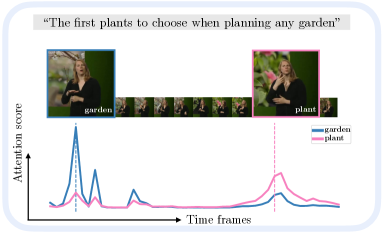
Figure 1: Sign localisation emerges from sequence prediction. In this work, we show that the ability to localise instances of signs emerges naturally by training a Transformer model [45] to perform a sequence prediction task on hundreds of hours of continuous signing videos with weakly-aligned subtitles.

Sign languages are visual languages that, for deaf communities, represent the natural means of communication [43]. Our goal in this paper is to identify and temporally localise instances of signs among sequences of continuous sign language. Achieving automatic sign localisation enables a diverse range of practical applications: construction of sign language dictionaries to support language learners, indexing of signing content to enable efficient search and intelligent fast-forward to topics of interest, automatic sign language dataset construction, wake-word recognition for signers [34] and tools to assist linguistic analysis of large-scale signing corpora.

In recent years, there has been a great deal of progress in temporally localising human actions within video streams [39, 51] and spotting words in spoken languages through aural [15] and visual [40, 30] keyword spotting methods. In both cases, a key driver of progress has been the availability of large-scale annotated datasets, enabling the powerful representation learning abilities of convolutional neural networks to be brought to bear on the task.

By contrast, annotated datasets for sign language are limited in scale and typically orders of magnitude smaller than their spoken counterparts [5]. Widely used datasets such as RWTH-PHOENIX [26, 9] and the CSL dataset [23] provide continuous sign annotations in the form of glosses or free-form sentences, but lack precise temporal annotations and are limited in content diversity, vocabulary, and scale. Large-scale collections of continuous signing videos exist, but are limited to sparse annotation coverage [2, 36].

In the absence of large-scale annotated training data, in this work we turn to a readily available and large-scale source: sign-interpreted TV broadcast footage together with subtitles of the corresponding speech in English. We propose to annotate this data with signs by training a Transformer [45] to predict, given input streams of continuous signing, the corresponding subtitles, and then using its trained attention mechanism to perform alignment from English words to signs.

This is a very challenging task: first, subtitles are only weakly aligned to the signing content—a sign may appear several seconds before or after its corresponding translated word appears in the subtitles, thus subtitles provide a relatively imprecise cue about the temporal location of a sign. Second, sign interpreters produce a translation of the speech that appears in subtitles, rather than a transcription—words in the subtitle may not correspond directly to individual signs produced by interpreters, and vice versa. Third, grammatical structures between sign languages and spoken languages differ considerably [43], and consequently the ordering of words in the subtitle is typically not preserved in the signing.

The core hypothesis motivating this approach is that in order to solve the sequence prediction task, the attention mechanism of the Transformer must be capable of localising sign instances. We demonstrate that by employing recent sign spotting techniques [2, 31] to coarsely align subtitles, sequence prediction is rendered tractable. One of the primary findings of this work is that, when performed at large scale (across hundreds of hours of continuous signing content), the ability to localise signs indeed emerges from the attention patterns of the sequence prediction model (Fig. 1).

We make the following four contributions: (1) by training on an appropriate sequence prediction task, we show that the attention mechanism of the Transformer learns to attend to specific signs, enabling their localisation; (2) we employ the learned attention to automatically generate hundreds of thousands of annotations for a large sign vocabulary; (3) we collect a set of 37K manually verified sign instances across a vocabulary of 950 sign classes to support our study of sign language recognition; (4) by training on the newly annotated data from our method, we outperform the prior state of the art on the BSL-1K sign language recognition benchmark.

2 Related Work

Our approach relates to prior work on sign language recognition, translation, spotting, and in particular automatic annotation of sign language data. We present a discussion of these, followed by a brief overview of Transformers in natural language processing (NLP) and works in other domains using attention mechanisms for localisation.

Sign language recognition and translation. The computer vision community has a long history of efforts to develop systems for sign language recognition, reaching back to the 1980s [44]. Initial work focused on hand-crafting features [44, 19] to model discriminative shape and motion cues and explored their usage in combination with Hidden-Markov Models [42, 46]. These works were followed by approaches that employed pose estimation as a basis for recognition [32, 33]. The community later transitioned to employing convolutional neural networks (CNNs) for appearance modelling [8]. In particular, the I3D architecture, originally developed for action recognition [12], has proven to be effective for sign recognition [27, 28, 24, 1, 30]—we similarly employ this model in our work.

Continuous sign language recognition entails important challenges compared to isolated sign recognition, including epenthesis effects and co-articulation [5] as well as the non-trivial definition of temporal boundaries between signs [6]. Towards dealing with these problems, [14] uses the CTC loss [21] to infer an alignment between sequence-level annotations and visual input and introduces an auxiliary loss to use the alignments as pseudolabels; while [7] proposes a graph convolutional network to automatically segment large sign language video sequences into short sentences, aligned with their subtitle transcription.

Recent works have applied sequence-to-sequence models to sign language translation. Camgöz et al. [9] use a two-stage pipeline that translates a video into gloss sequences then those into spoken language. Subsequent work [11] replaces this framework with a Transformer model trained on frame-level features jointly for recognition and translation, while [10] combines multiple articulators including face and upper body pose to train a translation system without gloss annotations. These approaches [9, 11, 10] have shown improvements towards translation in the restricted domain of discourse of the RWTH-PHOENIX-Weather-2014T German Sign Language (DGS) dataset [9]. Ko et al. [25] train a sequence-to-sequence model using keypoint features on Korean Sign Language translation. Although these methods show promising results in constrained conditions, open-vocabulary sign language translation in the wild remains largely unsolved.

Figure 2: Pipeline: We use an I3D model pretrained on sign classification to extract spatio-temporal visual features by using a sliding window. We then train a 2-layer Transformer model to predict stemmed subtitles from the input video feature sequence. We use the learned model’s attention vectors to spot new instances of signs by checking which words in the predicted hypothesis overlap with the stemmed subtitle. For example, here the tokens “talk” and “armi”, found in the model’s hypothesis, also appear in the subtitle and are therefore retained, while “know” does not and is hence discarded. The location of a new spotting is determined by the index at which the corresponding encoder-decoder attention peaks. Note: we omit the sample index, subscript $i$, shared by all variables (described in Sec. 3).

Automatic annotation of sign language data. Sign language datasets either offer isolated gloss-level annotations of single signs, e.g., MSASL [24], WLASL [27], or are heavily constrained in visual domain and vocabulary, e.g., RWTH-PHOENIX [26, 9], KETI [25] (only 105 sentences). Large-scale continuous sign language datasets, on the other hand, are not exhaustively annotated [2, 35]. The recent efforts of Albanie et al. [2] scale up the automatic annotation of sign language data, and construct the BSL-1K dataset with the help of a visual keyword spotter [41, 30] trained on lip reading to detect instances of mouthed words as a proxy for spotting signs. Sign spotting refers to a specialised form of sign language recognition in which the objective is to find whether and where a given sign has occurred within a sequence of signing. It has emerged as an intermediate step to collect more annotated sign language data. With this goal, Momeni et al. [31] use dictionary lookups in subtitled videos and improve low-shot sign spotting. Other automatic annotation approaches include an automatic pipeline for active signer detection and sign language diarisation [1]. While these previous methods are context-free, in this work, we introduce a context-aware approach that can be used to localise signs automatically. In fact, while we profit from annotations obtained in prior works using mouthing cues [2] and dictionaries [31], our approach differs considerably from theirs in method—we define the supervision directly on subtitles and formulate the problem as a sequence-to-sequence prediction task. We demonstrate the benefits of our approach empirically in Sec. 4.

Transformers in NLP. Incorporating an attention mechanism into encoder-decoder architectures led to a revolution in neural machine translation [4] by reducing dependency on strong text alignment. Vaswani et al. [45] further extended this approach by replacing all recurrent and convolutional components of a sequence-to-sequence model with self-attention. Even though such methods implicitly model source-to-target alignment with attention, their primary focus is on translation performance, rather than word-alignment. [20] further studies how to simultaneously optimise for accurate word-alignment without sacrificing translation performance—we investigate a variant of their approach in Sec. 4.

Attention mechanisms for localisation. Cross-modal attention has been employed in the literature for various localisation problems such as visual grounding in videos [48, 50, 29, 13] or images [17, 49], keyword spotting in audio [38] or visual speech [41, 30] and audio-visual sound source localisation [3, 37, 22]. However, to the best of our knowledge, our work is the first to apply these ideas at large-scale to sign localisation from weakly-aligned subtitles.

3 Sign Localisation with Attention

In this section, we describe how we train a Transformer model on a weakly-supervised sign language sequence-to-sequence task and then use the trained model to perform sign localisation (see Fig. 2 for an overview).

Let $\mathcal{X}_{\mathfrak{L}}$ denote the space of sign language video segments $\mathfrak{L}$, and $\mathcal{T}$ denote the space of subtitle sentences. Further, let $\mathcal{V}_{\mathfrak{L}}=~{}\{1,\dots,V\}$ represent the vocabulary (an enumeration of spoken language tokens that correspond to signs that can be performed in $\mathfrak{L}$) and let $\mathcal{S}$ denote a subtitled collection of $I$ videos containing continuous signing, $\mathcal{S}=\{(x_{i},s_{i}):i\in\{1,\dots,I\},x_{i}\in\mathcal{X}_{\mathfrak{L}},s_{i}\in\mathcal{T}\}$. Our objective is to localise potential occurrences of signs in $\mathcal{S}$.

Transformer training with subtitled videos. To address this task, we propose to train a sequence-to-sequence model with attention. Given a video-subtitle pair $(x_{i},s_{i})\in\mathcal{S}$, we train a Transformer [45] to predict the target text sequence $s_{i}=(s_{i}^{1},s_{i}^{2}\cdots,s_{i}^{T_{dec}})$ from the source video sequence $x_{i}=(x_{i}^{1},x_{i}^{2},\cdots x_{i}^{T_{enc}})$, one token at a time. Specifically, the Transformer’s encoder transforms $x_{i}$ into an encoded sequence $enc(x_{i})=(e_{i}^{1},e_{i}^{2},\cdots e_{i}^{T_{enc}})$. The decoder then attends on the encoded sequence and predicts the output sequence $\hat{s}_{i}=(\hat{s}_{i}^{1},\hat{s}_{i}^{2},\cdots\hat{s}_{i}^{T_{dec}})$ auto-regressively, factorising its joint probability into a product of individual conditionals:

$$p(\hat{s}_{i}|x_{i})=\prod_{t=1}^{T_{dec}}p(\hat{s}_{i}^{t}|{\hat{s}_{i}^{1},\hat{s}_{i}^{2}\cdots\hat{s}_{i}^{t-1}},enc(x_{i})).$$ (1)

Using the target subtitles $s_{i}$ as the ground truth output sequences, we train the model to maximise their log likelihoods by minimising the following loss:

$$\mathcal{L}=-\mathbb{E}_{(x_{i},s_{i})\in\mathcal{S}}\log p(s_{i}|x_{i})$$ (2)

Note that we assume access to a sparse collection of automatic sign annotations, $\mathcal{N}=\{(x_{k},v_{k}):k\in\{1,\dots,K\},v_{k}\in\mathcal{V}_{\mathfrak{L}},x_{k}\in\mathcal{X}_{\mathfrak{L}},\exists(x_{i},s_{i})\in\mathcal{S}\,s.t.\,x_{k}\subseteq x_{i}\}$, using mouthing cues [2] and dictionaries [31]. In practice, we restrict the Transformer training on a subset of videos $\mathcal{S}_{A}\subseteq\mathcal{S}$, containing at least one of these annotations within the subtitle timestamps, formally $\mathcal{S_{A}}=\{(x_{a},s_{a}):a\in\{1,\dots,A\},x_{a}\in\mathcal{X}_{\mathfrak{L}},\exists(x_{k},s_{k})\in\mathcal{N}\,s.t.\,x_{k}\subseteq x_{a}\}$. This ensures approximate alignment between the source video and target subtitle. For arbitrary sequences in $\mathcal{S}$ this is not guaranteed due to imperfect synchronisation between subtitles (corresponding to audio) and sign language interpretation. The goal of our training is therefore to exploit the knowledge of the unannotated words in the subtitles in $\mathcal{S}_{A}$ in order to discover a new collection of $(x,v)$ sign-video pairs (that is not included in $\mathcal{N}$) in the entire set $\mathcal{S}$.

Localising new sign instances with attention. Next, we describe how we use the Transformer model to look for new sign instances (see Fig. 2). After inputting the video sequence $x_{i}$ into the trained model, we use a decoding strategy (e.g., greedy) to predict the output sequence $\hat{s}_{i}$ and corresponding attention vectors $a_{i}=(\textbf{a}_{i}^{1},\textbf{a}_{i}^{2},\cdots\textbf{a}_{i}^{T_{dec}})\in R^{T_{dec}\times T_{enc}}$. We iterate over the predicted sequence $\hat{s}_{i}$ and localise new sign instances only for the tokens predicted correctly (i.e., appearing in subtitle $s_{i}$); the video location is determined by the index at which the corresponding attention vector is maximised, to yield sets of (location, sign) pairs of the form: $\{(\text{argmax}_{j\in\{1,2\cdots T_{enc}\}}\textbf{a}_{i}^{t}(j),s_{i}^{t}):\hat{s}_{i}^{t}=s_{i}^{t},t\in\{1,2\cdots T_{dec}\}\}$.

Implementation details. We represent the input video $x_{i}$ with features extracted using a pretrained spatio-temporal convolutional neural network model, applied in a sliding window manner with a 4-frame stride. In particular, we train an I3D architecture [12] on an extended set of automatic annotations $\mathcal{N}$ that we obtain by combining the methods of [2] and [31], to spot signs via mouthing cues and sign language dictionaries, respectively. We train with a single-sign classification objective and follow the same hyperparameters (e.g., 16-frame inputs) of the sign language recognition models in [2]. The 1024-dimensional video features from I3D are used as input to the Transformer encoder.

To construct ground-truth text labels for our Transformer training, we stem the words in every subtitle under the assumption that variations of a written word could map to the same sign. We note that the many-to-many mapping between words and signs is a complex problem, which we do not explicitly deal with in this work. To establish a tractable problem, we define a vocabulary of 11,515 stems based on their frequency and occurrence within the automatic annotations $\mathcal{N}$. This is reduced from an original set of 40K words appearing in the full set of subtitles $S$. We further remove stop words for which there is often no sign correspondence. This approach resembles glossing sign language data, i.e., representing sign sequences with word sequences, without spoken language grammar.

Following common practice in the sequence-to-sequence literature [45], we train the model with teacher forcing [47], i.e. at every decoding step we provide the previous-step’s ground truth as input to the decoder. During inference we experiment with three different decoding strategies: auto-regressive greedy decoding, left-to-right beam search, and teacher forcing. With greedy decoding, we iterate over the available sequences and for each one, we select as new spottings all the words in the predicted hypothesis that appear in the reference subtitle. For beam search, we iterate over the predictions which overlap with the reference from the multiple returned hypotheses, and select for each predicted word the location with maximum attention score. We show results for another variant of beam search where we choose the hypothesis with the highest recall in the appendix (Sec. C.3). With teacher forcing, we do not use the token predictions of the model, but only the attention scores, which we associate with the next ground-truth word in the subtitle at every decoding step. Since we consider all words in the subtitles, this strategy provides good yield but no notion of the model’s confidence. In order to obtain a confidence score we use the following heuristic: For every sequence, a word found in the subtitle is automatically annotated if the attention peak for the corresponding decoding step is higher than a threshold $\tau$.

When using Transformers with multiple attention heads, we obtain single attention scores by averaging the attention vectors of the individual heads. In Sec. 4.3 we discuss results on combining attention from different decoder layers.

4 Experiments

This section is structured as follows: We first present the datasets used as well as the various training and evaluation protocols that we follow in our experiments (Sec. 4.1). Next, we show how we choose our pretrained input video features (Sec. 4.2). Then, we evaluate our Transformer models trained with these features and discuss different strategies for mining new instances to obtain an automatically annotated training set (Sec. 4.3). We show that, when adding our newly mined training samples, we outperform the previous state of the art on sign language recognition (Sec. 4.4). Finally, we provide qualitative results on two datasets (Sec. 4.5) and discuss limitations (Sec. 4.6).

4.1 Data and evaluation protocols

Datasets. We use BSL-1K [2], a large-scale, subtitled and sparsely annotated dataset (for a vocabulary of 1,064 signs) of more than 1000 hours of continuous signing from sign language interpreted BBC television broadcasts. The programs cover a wide range of genres: from medical dramas and nature documentaries to cooking shows. In Sec. 4.5, we show qualitative examples on the RWTH-PHOENIX [9] dataset, which is significantly smaller in size and from weather broadcasts only, restricting the domain of discourse.

		Test${}^{\text{Rec}}_{2K}$ [2]				Test${}^{\text{Rec}}_{37K}$
		2K inst. / 334 cls.				37K inst. / 950 cls.
		per-instance		per-class		per-instance		per-class
Training	#ann.	top-1	top-5	top-1	top-5	top-1	top-5	top-1	top-5
M [2]$\mathsection$	169K	76.6	89.2	54.6	71.8	26.4	41.3	19.4	33.2
D	510K	70.8	84.9	52.7	68.1	60.9	80.3	34.7	53.5
M+D	678K	80.8	92.1	60.5	79.9	62.3	81.3	40.2	60.1

Table 1: A new recognition test set Test${}^{\text{Rec}}_{37K}$ and an improved I3D model: We employ the method of [31] to find signs via automatic dictionary spotting (D), significantly expanding the training and testing data obtained from mouthing cues by [2] (M). We also significantly expand the test set by manually verifying these new automatic annotations from the test partition (Test${}^{\text{Rec}}_{2K}$ vs Test${}^{\text{Rec}}_{37K}$). By training on the extended M+D data, we obtain state-of-the-art results, outperforming the previous work of [2] and providing strong I3D features for the subsequent steps of our method. $\mathsection$The slight improvement in the performance of [2] over the original results reported in that work is due to our denser test-time averaging when applying sliding windows (8-frame vs 1-frame stride).

Transformer training and evaluation on Test${}^{\text{Loc}}_{7K}$. To form the video-subtitle training data pairs, we sample 183K ($\mathcal{S}_{A}$) out of 685K subtitles from the BSL-1K training set ($\mathcal{S}$), in which there exists at least 1 automatic annotation (with a confidence score above 0.7) from the annotations collection $\mathcal{N}$. $\mathcal{N}$ is formed by applying the method of [2] on a large vocabulary of words beyond 1K to find signs via mouthing cues and applying the method of [31] to find signs via automatic dictionary spotting. See appendix (Sec. D.1) for details on this step. Subtitles originally contain 9.8 words from the initial 40K words vocabulary on average, which is reduced to 4.4 words per subtitle from the 11K stems vocabulary after stemming and filtering. Corresponding videos are tightly extracted according to the subtitle timestamps, and are on average 3.52 seconds long.

For evaluating the localisation capability of the proposed method, we use the automatic annotations $\mathcal{N}$ in the BSL-1K test set whose confidence scores are above 0.9, resulting in 7497 subtitle-video pairs with a total of 7661 annotations, referred to as Test${}^{\text{Loc}}_{7K}$. We measure the localisation accuracy for the annotated words in each subtitle and only on the correct predictions: we consider a correct prediction to be also correctly localised if its predicted location lies within 8 frames of the annotation time. We also report recall and precision of the model’s predictions for each sequence by measuring the percentage of words in the subtitle that are predicted (recall) and the percentage of predicted words which appear in the subtitle (precision). For all three metrics, we report the average over all sequences in the test set.

Single-sign recognition benchmark. In order to justify the value of our automatic annotation approach with the Transformer model, we evaluate on the proxy task of single-sign recognition on trimmed videos by using our localised sign instances from the training set as labels for classification training. Similar to [2, 24, 27], we adopt top-1 and top-5 accuracy metrics reported with and without class-balancing.

We use the BSL-1K manually verified recognition test set with 2K samples [2], which we denote with Test${}^{\text{Rec}}_{2K}$, and significantly extend it to 37K samples as Test${}^{\text{Rec}}_{37K}$. We do this by collecting new annotations from human annotators using the VIA tool [18] with a verification task as in [2]. This extended test set reduces the bias towards signs with easily spotted mouthing cues (since we also include dictionary spottings [30]) and spans a larger fraction of the training vocabulary, i.e. 950 out of 1064 sign classes (vs 334 classes in the original benchmark Test${}^{\text{Rec}}_{2K}$ of [2]).

4.2 Comparison of video features

We first conduct experiments to determine which I3D video features are best suited as input to the Transformer model as described in Sec. 3. In Tab. 1, we demonstrate the benefits of combining annotations from both mouthing (M) [2] and dictionary spottings (D) [31]. We show that our sign classification training using 678K automatic annotations obtains state-of-the-art performance on Test${}^{\text{Rec}}_{2K}$, as well as our new and more challenging test set Test${}^{\text{Rec}}_{37K}$. We therefore use this M+D model for the rest of our experiments. Note that all three models in Tab. 1 (M, D, M+D) are pretrained on Kinetics [12], followed by video pose distillation as described in [2]. We observed no improvements when initialising M+D training from M-only pretraining.

			Loc. Acc. (GD)		Loc. Acc. (TF)
Tr.	Recall	Prec.	Att. layer 1/2/3	[avg]	Att. layer 1/2/3	[avg]
1L	15.8	36.4	65.9	[65.9]	44.8	[44.8]
2L	16.5	37.2	63.9/57.8	[66.1]	51.1/37.6	[44.5]
3L	16.5	36.9	62.5/60.8/16.4	[65.3]	51.4/38.4/15.7	[46.4]

Table 2: Localisation performance of attention layers. We evaluate the performance of Transformers on Test${}^{\text{Loc}}_{7K}$ for different number of encoder/decoder layers in the training (different rows). We report the localisation accuracy for the encoder-decoder attention scores from every layer, as well as the average over layers, for both teacher forcing (TF) and greedy decoding (GD) modes.

4.3 Mining training examples through attention

Next, we ablate different design choices for the Transformer model.

Which attention layer for sign-video alignment? Similarly to [20], we conduct an investigation into which decoder layer gives attention scores that are more useful for localising signs. We train three models, with 1, 2 and 3 encoder and decoder layers and report the localisation accuracy when using the attention from each layer separately, or an average of all layers. The results on Test${}^{\text{Loc}}_{7K}$ in Tab. 2 suggest that averaging the attention scores over all layers gives the best localisation when using greedy auto-regressive decoding, while using the attention scores from the first decoder layer works best with teacher forcing. We note that this finding stands in contrast to those of [20] which concluded that the penultimate layer works better for word alignment in a machine translation task. We conjecture that the difference results from the different nature of the two domains, i.e., video versus text inputs. In terms of precision and recall, all three models perform similarly with rates at 37% and 16%, respectively. We continue with a 2-layer Transformer model for the rest of the experiments and given the observations in Tab. 2, we use the layer-averaged attention with greedy decoding and the first layer attention with teacher forcing.

Incorporating sparse annotations. As explained in Sec. 3, we make use of the available sparse annotations $\mathcal{N}$ to restrict the training subtitles to those with at least 1 annotation. When removing this constraint, the model does not train as well, and reaches a recall of only 6.8% (vs 16.5%).

Here, we also report some of our findings by employing three additional strategies to improve the Transformer training using the sparse annotations $\mathcal{N}$. In all three cases, we observe no or minor gains (on Test${}^{\text{Loc}}_{7K}$), at the cost of a more complex method and the need for annotations. Therefore, we do not integrate them in our final model and provide detailed results in appendix (Sec. C.2).

Alignment loss on sparse annotations: We investigate whether the sparse annotations $\mathcal{N}$ could be used for supervising the sign-video alignment explicitly (similar to [20] in NLP). To this end, we define an additional loss that operates on the encoder-decoder attention to enforce a high response whenever there is known location information. We achieve this via an additional L2 loss term between a 1D gaussian centered around the annotated time frame and the corresponding attention vector. While the localisation performance with teacher-forcing increases (58.7% vs 51.1%), it still remains lower compared to the corresponding greedy decoding result and we observe no significant gains for other metrics measured on the predictions.

Curriculum learning with sparse annotations: To provide warmup for the model training, we start by temporally trimmed video inputs around known sign locations $\mathcal{N}$. We gradually increase the number of annotations from 1 to 3, before we fully input the subtitle duration to the Transformer. We only observe minor improvements: 16.0% vs 15.8% recall with the 1-layer architecture.

Subtitle alignment through active signer detection and sparse annotations: To overcome the alignment noise present in the data, we apply an algorithm that combines a pose-based active signer detection [1] and the knowledge of sparse annotations $\mathcal{N}$. Specifically, we apply temporal shifts to subtitles such that their temporal midpoint aligns with the average time of any annotated signs they contain. We then apply affine transformations to the subtitles without annotations such that they fill the regions between those with annotations, subject to the hard constraint that the expansions do not overlap periods of inactive signing. This approach increases the amount of training subtitles with annotations to 230K; however, training with this new set does not improve recall (15.4% vs 16.5% with 2-layers).

	#subtitles	#ann.	#ann.	top-1	top-1
Spotting mode	unannot.	11K	1K	per-inst	per-cls
TF ($\geq.2$)	114K	290K	97K	22.2	4.7
TF ($\geq.1$)	408K	1.7M	545K	37.3	13.4
TF ($\geq.05$)	457K	2.3M	754K	38.7	14.4
TF ($\geq.05$) (align. loss)	457K	2.3M	757K	38.8	14.6
BS (10 best)	109K	329K	166K	49.6	22.7
GD (no subtitle filtering)	480K	1.4M	910K	50.6	22.6
GD (align. loss)	53K	188K	108K	53.6	24.8
GD	53K	188K	107K	53.9	24.7

Table 3: Automatically annotating the training data: We show the yield obtained from various decoding strategies in terms of number of additional annotations (left). Training models only with these annotations, we evaluate the recognition accuracy on Test${}^{\text{Rec}}_{37K}$. Greedy decoding (GD) obtains better results than teacher forcing (TF) even when not filtering the predictions against the ground-truth subtitles. Neither including 10 best predictions from beam search (BS) nor using the model trained with the alignment loss influences the recognition evaluation significantly.

Which decoding mechanism? To form a new annotated set for sign recognition training, we apply the trained Transformer models on the whole 685K training video-subtitle pairs of the BSL-1K dataset. In Tab. 3 we summarise and compare the yield of new training samples mined with the different decoding strategies we discussed in Sec. 3. We report the number of previously unannotated subtitles, for which the attention mechanism is able to localise signs, to demonstrate the benefits of our approach. We also report the amount of new annotations for both the full 11K vocabulary and the 1064-subset which is used for the proxy recognition evaluation. We observe that a significant number of new automatic sign annotations are obtained with our approach.

To compare the different decoding strategies, we train recognition models on the resulting training sets containing the new annotations and evaluate them on the proxy sign recognition task. Note that for faster training, we learn a 4-layer MLP architecture on top of the pre-extracted I3D video features (architecture and optimisation details are given in the appendix, see Sec. D).

We observe that greedy decoding with the simple filtering mechanism (checking against ground truth) gives best downstream recognition performance on Test${}^{\text{Rec}}_{37K}$. Teacher forcing, beam search and no filtering all yield larger but noisier training sets that result in lower performance. However, we note that the “no subtitle filtering” experiment assumes no access to ground-truth subtitles during annotation mining and uses all the predictions, while providing competitive recognition performance (50.6% vs 53.9%).

		per-instance		per-class
Training	#ann.	top-1	top-5	top-1	top-5
A	107K	54.0±0.08	67.9±0.10	24.8±0.10	35.5±0.20
M [2]$\dagger$	169K	40.8±0.17	62.2±0.07	21.7±0.19	38.5±0.29
M+A	276K	58.5±0.17	75.5±0.02	30.4±0.04	45.9±0.26
D [31]$\dagger$	510K	62.1±0.24	80.8±0.10	35.1±0.38	54.3±0.11
D+A	276K	64.2±0.08	81.7±0.07	36.0±0.26	54.0±0.32
M+D	678K	63.5±0.28	82.1±0.04	37.2±0.12	56.4±0.17
M+D+A	786K	65.0±0.14	82.6±0.02	37.9±0.07	56.3±0.02

Table 4: Sign recognition on BSL-1K Test${}^{\text{Rec}}_{37K}$: We evaluate our 4-layer MLP classification models trained on video feature inputs for 1064-sign recognition for various training label sets: mouthing (M), dictionary (D), and our proposed attention (A) spottings. We obtain state-of-the-art results, by consistently improving over previous works when including our attention localisations. $\dagger$The results are obtained from our MLP trained with the annotations from [2] and our application of [31].

4.4 Comparison with other automatic annotations

In this section, we train for sign recognition on BSL-1K [2] on various label sets, comparing different automatic annotation methods and showing that our new sign instances are complementary when added to training data, achieving state of the art. As in the previous experiments, we use the MLP architecture on frozen I3D features to compare the different annotation sets. This time we perform 3 trainings per model with different random seeds and report the average and standard deviation.
Tab. 4 summarises the results on Test${}^{\text{Rec}}_{37K}$. We first note that the MLP performance of M+D annotations matches and slightly outperforms that of I3D from Tab. 1 (63.5% vs 62.3%), validating the suitability of MLP for efficiently comparing annotation set quality. When compared to the visual keyword spotting through mouthing (M) [2], our automatic attention localisations (A) show significant improvements. Furthermore, we observe consistent improvements when combining our new annotations with either the mouthing (M+A) or dictionary (D+A) annotations. Combining all available annotations (M+D+A), we achieve state-of-the-art performance (65%) outperforming previous work of [2] (M: 40.8%), as well as a new much stronger baseline (D: 62.1%) that we establish in this work, which uses the new annotations obtained using sign language dictionaries for sign spotting [31]. Our final recognition model can be interpreted as distilling information from multiple sources (mouthing, dictionary, attention), each of which has access to a large training set.

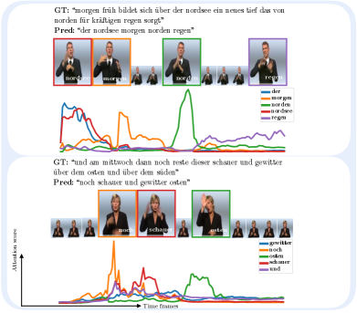
Figure 3: Qualitative analysis on the RWTH-PHOENIX: We show example sign localisation results on the test set of RWTH-PHOENIX 2014T. For each video clip, we show the ground-truth sentence as well as the predicted words from the Transformer model of [11] which overlap with the target sentence. We plot attention scores over time frames for these predicted words and show the frame index at which the corresponding attention vector is maximised for a subset of the correctly predicted words.

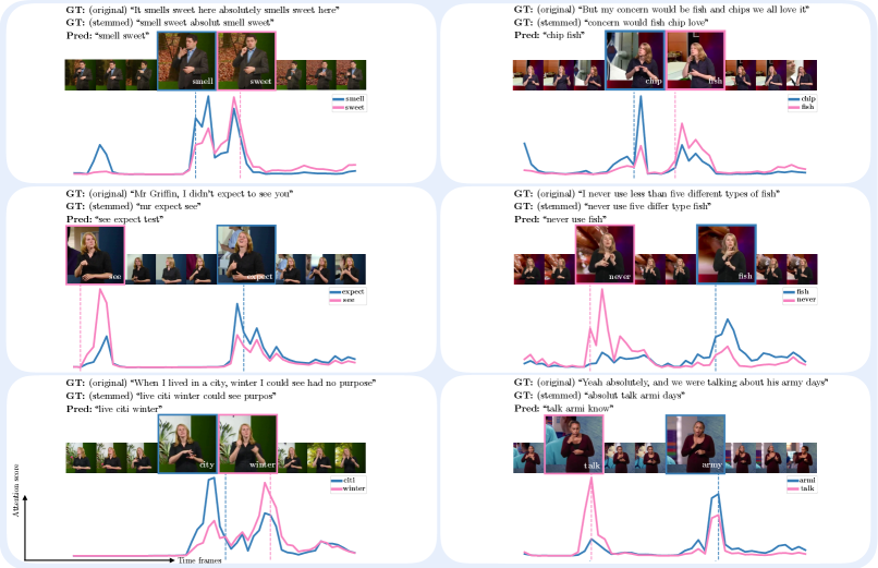
Figure 4: Qualitative analysis on BSL-1K: We show example sign localisation results on the BSL-1K test set (Test${}^{\text{Loc}}_{7K}$). For each video clip, we show the original subtitle, the ground-truth stemmed and filtered to 11K vocabulary version, and the prediction of our Transformer model. We plot attention scores over time frames for the predicted words which overlap with the subtitle and for which we have annotated sign times in $\mathcal{N}$ (shown by vertical dashed lines). We highlight the frame at which the corresponding attention vector is maximised.

We also evaluate the performance of our MLP trained on M+D+A annotations on the BSL-1K sign spotting benchmark proposed by [2], following their protocol, and achieve a score of 0.174 mAP, outperforming the previous state-of-the-art performance of 0.170 mAP [31] and 0.159 mAP [2].

4.5 Qualitative analysis

We demonstrate the potential of our Transformer model to localise sign instances through its attention mechanism. Fig. 4 shows qualitative examples of localising multiple signs, by plotting attention scores over video time frames for predicted words that occur in corresponding subtitles of the BSL-1K test set (Test${}^{\text{Loc}}_{7K}$). We observe close alignment with the automatic annotations $\mathcal{N}$. One potential limitation of this approach for localisation is that the attention vector does not peak only at the corresponding sign location, but also on other signs suggesting that the predictions use context (e.g., “smell” and “sweet” in Fig. 4, top-left).

We also investigate whether this localisation ability extends to other datasets. In particular, we reproduce the translation method of Camgöz et al. [11] on RWTH-PHOENIX 2014T [9] and similarly to [9], we visualise the attention score plots for predicted words in Fig. 3. We are unable to compute the localisation accuracy as sign annotation times are not available for RWTH-PHOENIX 2014T; however, we observe correct signs when indexing the frame at which the corresponding attention vector is maximised. This suggests that alignment emerges from the attention mechanism also for a full translation system.

4.6 Discussion

From our investigations in this work, we believe there are important and challenging problems to be solved before achieving large-vocabulary sign language translation from videos to spoken language. First, significantly expanding the coverage of the vocabulary of both languages is necessary, and the current state of the art only covers about 3K spoken language and 1K sign language vocabularies [11]. In preliminary experiments, we found that a direct application of [11] to translation on the significantly broader vocabulary of 40K contained within the subtitles of BSL-1K failed to converge to meaningful results (for more details see appendix, Sec. C.1). In this work, we have extended to an 11K spoken language vocabulary, but the NLP literature typically works with much larger vocabularies (e.g. a few hundred thousand words [16]). Our attempts to move to 40K words did not obtain sufficient-quality results. Second, the alignment between text and video is far from perfect in large-scale sign language datasets which inserts significant amount of noise in training. Our automatic alignment attempts in this work did not obtain improvements. Relying on sparse annotations for approximate alignments limits the amount of data. Third, most of the works, including ours, focus on interpreted data, which has certain biases. In fact, the act of interpreting can cause a simplification in signing style and vocabulary, and even lead to a reduction in speed for comprehension  [5]. Datasets of native signers should be built to train strong, robust models that generalise at scale and in the wild. Given these observations, we believe that future work that specifically targets translation systems will benefit from addressing these challenges. We refer to the appendix (Sec. A) for a discussion of broader impact.

5 Conclusions

We have presented an approach to localise signs in continuous sign language videos with weakly-supervised subtitles by leveraging the attention mechanism of a Transformer model trained on a video-to-text sequence prediction task. We find that state-of-the-art translation models have very low recall on a large-vocabulary dataset, but a satisfactory localisation accuracy through attention that allows us to annotate sign timings. We automatically annotate hundreds of thousands of new signing instances through our learned attention and validate their quality by using them to train a sign language recognition model that surpasses the state of the art on the BSL-1K benchmark as well as a more robust sign language benchmark which is 18 times larger. Future work can leverage our automatic annotations and recognition model for large-vocabulary sign language translation.

Acknowledgements. This work was supported by EPSRC grant ExTol and a Royal Society Research Professorship. We thank Cihan Camgöz, Himel Chowdhury and Abhishek Dutta for their help.

APPENDIX

This appendix to the main paper provides a discussion on broader impact (Sec. A), additional qualitative (Sec. B) and quantitative results (Sec. C), as well as implementation details (Sec. D).

Appendix A Broader impact

At present, computer vision technology to usefully assist signers remains in its infancy. In large part, this stems from the high difficulty of achieving robust machine comprehension of sign language, which falls a long way short of human performance [5]. Our work, which focuses specifically on sign localisation, takes steps towards enabling several practical applications that may become viable even when a full automatic understanding of sign language remains incomplete. These include: (1) sign language dictionary construction to assist students who wish to learn sign language, (2) index construction for video corpora, allowing individuals to search videos by the content of their signing, (3) wake-word spotting for signing users of smart assistants like Alexa and Siri, (4) tools for linguists to assist in the efficient analysis of existing signing data and (5) automatic large-scale dataset construction to facilitate future research towards technology that will ultimately be able to provide useful products and services to the Deaf community.

The development of automatic, accurate sign localisation also has risks. Notably, It has the potential to be used for surveillance. Moreover, as with many computer vision methods employing deep neural networks (as ours does), the model is prone to fitting the training distribution closely. As a result, it will be vital that products and services employing this technology ensure that their users are well-represented in the training data to avoid a disparity of performance across groups.

Appendix B Qualitative results

We refer to our supplementary video at our project webpage for additional visual results and illustrations. First, we visualise the attention scores for sample test videos, similarly to Fig. 4 of the main paper. To make it easier to assess the localisation quality visually, we show an example dictionary video corresponding to the localised sign. Next, we demonstrate the capability to temporally localise signs in long continuous videos using this attention mechanism on a training sequence. Finally, we present our automatic annotations on the training set (that we obtain through checking against subtitles), which we use for sign language recognition training. When grouping videos corresponding to the same word, we observe a temporal alignment across samples.

Appendix C Additional experimental results

We provide additional quantitative analysis through experimentation with different subtitle preprocessing approaches (Sec. C.1), a detailed breakdown of performance for methods incorporating sparse annotations (Sec. C.2), additional decoding strategies to mine training examples (Sec. C.3), and a recognition architecture study (Sec. C.4).

C.1 Subtitle processing

All experiments in this section are reported on Test${}^{\text{Loc}}_{7K}$ to evaluate the Transformer training for the sequence prediction task.

Stemming. We experiment with stemming versus using the original subtitle words in Tab. A.1. The 11K annotation stems correspond to a vocabulary of 16K words. We train a model by filtering the subtitles to these 16K words without any further processing. We observe no significant differences between the two models. Note that, for a fair comparison, we stem the words at evaluation time.

	vocab.	Recall	Prec.	LocGD	LocTF
Stemming	11K	16.5	37.2	66.1	44.5
No stemming	16K	16.0	35.5	66.8	52.3

Table A.1: Stemming subtitles: We find that stemming might not be necessary for training. Note that for both models, we stem the words at evaluation.

% of subtitle	train	test	#test
vocabulary	vocab.	vocab.	subtitles	Recall	Prec.	LocGD	LocTF
100%	26K	26K	7588	14.9	35.6	67.9	49.9
		11K(11K)	7497	15.9	36.0	68.0	50.2
75%	19K	19K	7567	15.2	36.0	67.7	38.9
		11K(10K)	7497	16.2	36.3	67.8	39.6
50%	13K	13K	7516	15.9	36.8	66.6	52.4
		11K(9K)	7497	16.7	36.9	66.7	52.3
25%	6K	6K	7271	17.0	40.0	66.3	52.0
		11K(6K)	7497	17.0	39.0	66.6	51.8
Annot. vocab.	11K	11K	7497	16.5	37.2	66.1	44.5

Table A.2: Vocabulary size: We systematically change the training vocabulary of stems by taking subsets of the full subtitle vocabulary. We take the top 25%, 50%, 75%, 100% of stems according to their frequencies in the subtitles. Each trained model is tested twice (two rows per model): with (a) the same vocabulary used for training, (b) the comparable 11K vocabulary used in the rest of the experiments. Note that in (b), there might not be a full overlap between the train and test; the numbers in parenthesis represent the intersection.

Vocabulary. In this work, we have used a vocabulary of 11K stems which is determined based on the annotations. In Tab. A.2, we train additional Transformer models by using vocabularies determined by the subtitles. We sort the stems appearing in all subtitles based on their frequencies. We train with top 25%, 50%, 75%, 100% of all stems. We observe that the models are not very sensitive to the choice of training vocabulary. Note that in all cases, we filter out the stop words which do not have sign correspondences.

	vocab.	Recall	Prec.	LocGD	LocTF
Without stop words	11K	16.5	37.2	66.1	44.5
With stop words	11K	13.9	25.9	69.5	52.5

Table A.3: Removing stop words: We train a model by including the stop words (although these rarely have corresponding signs), and obtain lower performance (13.9% recall).

train	test	#test
vocab.	vocab.	subtitles	Recall	Prec.	LocGD	LocTF
40K	40K	7413	9.5	7.5	70.3	27.1
40K	16K	7299	10.3	7.5	70.3	27.0

Table A.4: Naive translation with 40K vocabulary: We report the results of training a model without stemming and without vocabulary filtering (except we filter to the 260K English vocabulary of Transformer-XL to remove the noise in the subtitles, due to OCR mistakes etc.). We test the model on (a) the same 40K vocabulary used for training, and (b) the 16K subset covering the annotations. Overall, we observe poor precision and recall.

Stop words. In Tab. A.3, we train one model by keeping the stop words and compare against our model. Note that we determine the list of stop words according to English stop words in the nltk.corpus. Qualitatively, we observe frequent occurrence of the words “and” and “to” in the predictions. The precision and recall metrics reflect the reduced quality of the outputs as well. Therefore, we filter out the stop words in all other models.

Naive translation. Tab. A.4 reports results for training a model with a large vocabulary, without filtering and without stemming. We again stem the words at evaluation time. We observe poor performance and highlight the difficulty of the translation problem on in-the-wild sign language data. A few qualitative predictions are provided below. We note that while some examples have overlap between ground truth and prediction (#1, #2, #3), many examples repeat the same prediction (#4, #5), or output frequent words (#6). As argued in the discussion section of the main paper (Sec. 4.6), we believe that the video-text alignment and large-vocabulary sign recognition problems should become more advanced to achieve in-the-wild translation.

     Example #1  Reference:  through your own admission your last  time in the competition  Hypothesis: the competition is a competition    Example #2  Reference:  lots of water to help digest such a meal  Hypothesis: and then the water is the water    Example #3  Reference:  people talk you see  Hypothesis: i think the people were a good    Example #4  Reference:  and just tease out the dead growth  Hypothesis: and the whole thing is a little bit    Example #5  Reference:  and how little we knew about the species  Hypothesis: and the whole thing    Example #6  Reference:  wrong here again going to give it how many  Hypothesis: i think that is a good     

C.2 Incorporating sparse annotations

As in Sec. C.1, all experiments in this section are reported on Test${}^{\text{Loc}}_{7K}$.

Alignment loss on sparse annotations. Tab. A.5 presents detailed results on the incorporation of the alignment loss as described in Sec. 4.3 of the main paper. Although minor improvements are observed with the addition of such a loss term, we do not use it in the final model for simplicity.

				Loc. Acc. (GD)		Loc. Acc. (TF)
$\lambda_{\mathcal{L}_{align}}$	L	Recall	Prec.	layer 1/2	[avg]	layer 1/2	[avg]
0	-	16.5	37.2	63.9/57.8	[66.1]	51.1/37.6	[44.5]
10	avg	16.8	37.5	64.7/59.2	[66.0]	51.4/36.1	[45.2]
100	avg	16.4	37.2	67.4/60.7	[68.0]	52.8/42.3	[48.0]
1000	avg	14.4	34.5	68.9/59.0	[67.3]	52.5/55.8	[56.6]
10	1	16.8	38.3	62.9/63.8	[66.4]	51.2/40.7	[43.1]
100	1	16.7	37.3	67.5/63.6	[66.7]	52.9/38.5	[42.1]
1000	1	15.7	33.5	59.4/69.8	[69.6]	57.0/35.6	[48.7]
10	2	16.8	37.4	65.8/59.2	[67.3]	51.7/36.8	[47.1]
100	2	16.2	37.7	68.5/57.2	[68.0]	46.0/50.4	[47.5]
1000	2	14.8	35.5	67.1/59.2	[66.3]	42.5/58.7	[53.6]

Table A.5: Alignment loss on sparse annotations: We experiment with different weighting terms for the alignment loss ($\lambda_{\mathcal{L}_{align}}$) in addition to the classification loss during subtitle training. We define the loss on various attention layers (L) of a 2-layer architecture. We observe minor improvements.

Curriculum learning with sparse annotations. Tab. A.6 reports results with and without the curriculum strategy described in Sec. 4.3 of the main paper. We obtain minor improvements with pretraining the Transformer on shorter temporal segments containing only 1 annotated sign, finetuning the model later on 2 and 3 signs. Note that this model uses 1 layer in both encoder and decoder unlike other experiments which use 2 layers (we note from our Transformer layer ablations reported the main paper that this does not dramatically affect localisation performance).

Training schedule	Recall	Prec.	LocGD	LocTF
No curriculum: Subtitle	15.8	36.4	65.9	44.8
With curriculum: 1$\rightarrow$2$\rightarrow$3$\rightarrow$Subtitle	16.0	37.1	66.6	44.3

Table A.6: Curriculum learning with sparse annotations: We observe minor improvements by incorporating curriculum learning, which gradually extends the temporal window of the input video. Note that a 1-layer encoder-decoder architecture is used for this experiment.

Training subtitles	Recall	Prec.	LocGD	LocTF
662K not aligned	6.8	16.3	67.1	27.0
183K not aligned (subset)	6.2	15.0	65.4	25.5
230K aligned	15.4	38.3	66.7	51.5
301K coarse (pad $\pm$2-sec)	13.9	45.2	67.6	48.3
183K coarse	16.5	37.2	66.1	44.5

Table A.7: Subtitle-video alignment: Our coarse alignment, which uses the assumption that the subtitles that have at least one annotation within the subtitle timestamp is aligned with its video, obtains the best performance over other alignment variants or using no alignment.

Video-subtitle alignment. Tab. A.7 details our experiments which highlight the importance of video-subtitle alignment. When using all subtitles without considering whether they contain an annotation or not (662K subtitles), we obtain poor recall on the test set where there is at least one high-confidence ($\geq$0.9) annotation. To keep the number of training subtitles same as our final model, we also experiment with taking a random subset of 183K subtitles, and observe a similar outcome of poor performance. When using active signer detection and sparse annotations to apply a simple algorithm to align the subtitles, we get to 230K training subtitles that have at least 1 annotation; however, this model does not impact the results significantly. To take the uncertainty into account, we also experiment with padding $\pm$2 seconds at the start and end of the subtitle times to input more video features to the model. However, this model also reduces the recall. Our simple coarse alignment strategy of using subtitles that have at least 1 annotation results in the best performance.

C.3 Decoding strategies

In Sec. 4.3 of the main paper, we have described different decoding mechanisms to mine new training annotations by applying the Transformer model. Here, we provide two more strategies to complement Tab. 3 (a) 1 best: choosing the hypothesis with the highest recall when applying beam search with size 10, (b) TF prediction: decoding with teacher forcing and forming a hypothesis using the model’s prediction at every step, then filtering the hypothesis by only keeping the tokens that are also present in the corresponding subtitle (same as with GD); this is an alternative form of the TF baseline – here we also use the attentions of the first layer only. The new results are denoted with bold font in Tab. A.8 for Test${}^{\text{Rec}}_{37K}$. The best result is achieved by simple greedy decoding (GD) which has smaller but more noise-free sign localisations.

Fig. A.1 shows several training plots corresponding to different decoding mechanisms. The curves suggest that mining more examples with higher noise results in low training performance. The plotted metric is top-1 per instance accuracy over 30 training epochs.

C.4 Recognition architecture study

We present an experimental study for the architecture design of our MLP which is used for recognition. Tab. A.9 summarises the results on Test${}^{\text{Rec}}_{37K}$ for training with all M+D+A annotations, i.e., our best model in Tab. 4 of the main paper. While the results are not significantly different, we observe minor improvements with increased capacity, which quickly saturates when adding more layers.

	#subtitles	#ann.	#ann.	top-1	top-1
Spotting mode	unannot.	11K	1K	per-inst	per-cls
TF ($\geq.05$)	457K	2.3M	754K	38.7	14.4
BS (10 best)	109K	329K	166K	49.6	22.7
BS (1 best)	109K	316K	161K	50.7	23.3
TF prediction	57K	195K	110K	51.3	22.5
GD	53K	188K	107K	53.9	24.7

Table A.8: Other decoding strategies: TF: teacher-forced decoding, filtering with a threshold on attention scores; BS (10 best): beam search decoding with beam size 10 - all returned hypotheses are used when looking for new instances; BS (1 best): the same beam search is performed (with beam size 10) but only the hypothesis with the highest recall is used; TF prediction: teacher-forced decoding, using the hypothesis predicted by the model and checking against subtitle; GD: greedy decoding. The strategies shown in bold font refer to experiments not included in the main paper and are described in more detail in Sec. C.3. For the rest, we refer to Sec. 4.3 of the main paper.

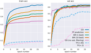
Figure A.1: Training recognition with attention spottings: We plot the training (left) and validation (right) accuracy curves against the epoch number for different MLP models, corresponding to different decoding strategies to mine training examples. The legend corresponds to descriptions in Tab. A.8 and Tab. 3 of the main paper. See Sec. C.3 and Sec. 4.3 of the main paper for details. We conclude that increased noise in teacher forcing mechanism (dashed), despite its large yield, makes learning difficult.

	per-instance		per-class
Architecture	top-1	top-5	top-1	top-5
1024$\rightarrow$res(1024)$\rightarrow$512$\rightarrow$256	65.1	82.6	38.0	56.4
1024$\rightarrow$512$\rightarrow$256	64.6	82.3	36.5	55.1
1024$\rightarrow$256	63.8	82.0	35.2	53.9
1024$\rightarrow$res(1024)$\rightarrow$512$\rightarrow$128	64.9	82.6	37.4	55.9
1024$\rightarrow$res(1024)$\rightarrow$512$\rightarrow$512	65.3	82.6	38.4	57.0
1024$\rightarrow$res(1024)$\rightarrow$512$\rightarrow$1024	65.5	82.9	39.0	57.4
1024$\rightarrow$res(1024)$\rightarrow$512	65.3	82.9	37.9	56.6
1024$\rightarrow$res(1024)$\rightarrow$512$\rightarrow$512$\rightarrow$1024	65.5	82.7	39.0	57.4
1024$\rightarrow$res(1024)$\rightarrow$512$\rightarrow$512$\rightarrow$512$\rightarrow$1024	65.0	82.4	38.3	57.1

Table A.9: Architecture study for recognition: We experiment with different number of layers for the sign recognition model. The input dimensionality is 1024, which is a temporally-averaged I3D embedding over 16 frames. The output is 1064-dimensional class probabilities. The top row is what is reported in the main paper (corresponding to Fig. A.2). We observe minor improvements by increasing the network capacity.

Appendix D Implementation details

D.1 Application of M [2] and D [30]

As explained in Sec. 4.1, we apply the method of [2] to localise signs through mouthing cues on a large vocabulary of words beyond 1K (which is used in the original work). In particular, we query 36K words, and out of these, a vocabulary of 15K words are localised with confidence above 0.7. When applying the method of [30] to localise signs through similarity matching with dictionary videos, we query 9K signs from the full BSLDict dataset with search windows of $\pm$4 seconds padding around the subtitle timestamps. The resulting sign localisations with confidence above 0.7 cover a vocabulary of 4K words. The combination of these two methods gives us a total vocabulary of 16K words, which results in the 11K stems used for our Transformer training.

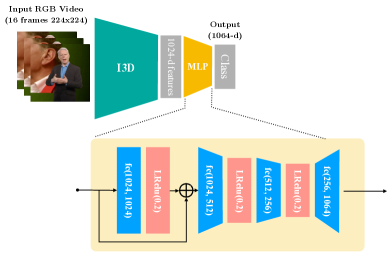
Figure A.2: MLP architecture for recognition: We follow [31], and use one residual connection, followed by 3 more fully connected layers on top of the I3D pre-extracted features.

D.2 Architecture and training details

Our Transformer model consists of 2 attention layers for both encoding and decoding. The input 1024-dimensional video feature is mapped to 512 dimensions with a linear layer. Then 512-d embeddings are used both for output words and input videos. We use 2 heads in each attention layer.

When reporting localisation accuracy, we average the encoder-decoder attention scores over the 2 heads. We take the first layer attention for teacher forcing (TF) and the average over two layers for greedy decoding (GD). We mark a correct localisation if the maximum location over the input video is within $\pm$2 feature frames from the annotation time. This is because one sign approximately lasts for 7-13 frames (at 25fps) [31] and our features are extracted with a stride of 4 frames, making our valid window duration $\pm$8 video frames. This also accounts for some uncertainty in the ‘ground-truth’ annotation times which are obtained automatically.

We detail our MLP architecture in Fig A.2. We use a design similar to [31]. The architecture study in Sec. C.4 reports variations of this model. We train it for 30 epochs, with an initial learning rate of $1e^{-2}$ reduced by a factor 10 at the 20th and 25th epoch.

D.3 Infrastructure

We use Nvidia M40 graphics cards for our experiments. The video-subtitle Transformer model trains in 10 hours on a single GPU. The annotation mining time is roughly 30 minutes to obtain 107K annotations, i.e., Transformer forward pass runtime over 1302h of training videos (duration of 685K subtitles padded with $\pm$2 seconds) on a single GPU. The final best MLP (M+D+A) for sign recognition trains in 7 hours on a single GPU. The M+D I3D backbone is trained with 4 GPUs over a duration of 1 week.

References

- [1] S. Albanie, G. Varol, L. Momeni, T. Afouras, A. Brown, C. Zhang, E. Coto, N. C. Camgöz, B. Saunders, A. Dutta, N. Fox, R. Bowden, B. Woll, and A. Zisserman. SeeHear: Signer diarisation and a new dataset. In ICASSP, 2021.
- [2] S. Albanie, G. Varol, L. Momeni, T. Afouras, J. S. Chung, N. Fox, and A. Zisserman. BSL-1K: Scaling up co-articulated sign language recognition using mouthing cues. In ECCV, 2020.
- [3] R. Arandjelovic and A. Zisserman. Objects that sound. In ECCV, 2017.
- [4] D. Bahdanau, K. Cho, and Y. Bengio. Neural machine translation by jointly learning to align and translate. In ICLR, 2015.
- [5] D. Bragg, O. Koller, M. Bellard, L. Berke, P. Boudreault, A. Braffort, N. Caselli, M. Huenerfauth, H. Kacorri, T. Verhoef, C. Vogler, and M. Ringel Morris. Sign language recognition, generation, and translation: An interdisciplinary perspective. In ACM SIGACCESS, 2019.
- [6] D. Brentari. Effects of language modality on word segmentation: An experimental study of phonological factors in a sign language. Papers in laboratory phonology, vol.8, pages 155–164, 2009.
- [7] H. Bull, M. Gouiffès, and A. Braffort. Automatic segmentation of sign language into subtitle-units. In ECCVW, Sign Language Recognition, Translation and Production (SLRTP), 2020.
- [8] N. C. Camgoz, S. Hadfield, O. Koller, and R. Bowden. Subunets: End-to-end hand shape and continuous sign language recognition. In ICCV, 2017.
- [9] N. C. Camgoz, S. Hadfield, O. Koller, H. Ney, and R. Bowden. Neural sign language translation. In CVPR, 2018.
- [10] N. C. Camgoz, O. Koller, S. Hadfield, and R. Bowden. Multi-channel transformers for multi-articulatory sign language translation. In ECCVW, 2020.
- [11] N. C. Camgoz, O. Koller, S. Hadfield, and R. Bowden. Sign language transformers: Joint end-to-end sign language recognition and translation. In CVPR, 2020.
- [12] J. Carreira and A. Zisserman. Quo vadis, action recognition? a new model and the kinetics dataset. In CVPR, 2017.
- [13] J. Chen, X. Chen, L. Ma, Z. Jie, and T.-S. Chua. Temporally grounding natural sentence in video. In EMNLP, 2018.
- [14] K. L. Cheng, Z. Yang, Q. Chen, and Y.-W. Tai. Fully convolutional networks for continuous sign language recognition. In ECCV, 2020.
- [15] A. Coucke, M. Chlieh, T. Gisselbrecht, D. Leroy, M. Poumeyrol, and T. Lavril. Efficient keyword spotting using dilated convolutions and gating. In ICASSP, 2019.
- [16] Z. Dai, Z. Yang, Y. Yang, J. Carbonell, Q. V. Le, and R. Salakhutdinov. Transformer-XL: Attentive language models beyond a fixed-length context. In ACL, 2019.
- [17] C. Deng, Q. Wu, Q. Wu, F. Hu, F. Lyu, and M. Tan. Visual grounding via accumulated attention. In CVPR, 2018.
- [18] A. Dutta and A. Zisserman. The via annotation software for images, audio and video. In ACMMM, 2019.
- [19] H. Fillbrandt, S. Akyol, and K.-F. Kraiss. Extraction of 3D hand shape and posture from image sequences for sign language recognition. In SOI, 2003.
- [20] S. Garg, S. Peitz, U. Nallasamy, and M. Paulik. Jointly learning to align and translate with transformer models. In EMNLP, 2019.
- [21] A. Graves, S. Fernández, F. Gomez, and J. Schmidhuber. Connectionist temporal classification: labelling unsegmented sequence data with recurrent neural networks. In ICML, 2006.
- [22] D. Harwath, A. Recasens, D. Surís, G. Chuang, A. Torralba, and J. Glass. Jointly discovering visual objects and spoken words from raw sensory input. In ECCV, 2018.
- [23] J. Huang, W. Zhou, Q. Zhang, H. Li, and W. Li. Video-based sign language recognition without temporal segmentation. In AAAI, 2018.
- [24] H. R. V. Joze and O. Koller. MS-ASL: A large-scale data set and benchmark for understanding American Sign Language. In BMVC, 2019.
- [25] S.-K. Ko, C. J. Kim, H. Jung, and C. Cho. Neural sign language translation based on human keypoint estimation. Appl. Sci., 2019.
- [26] O. Koller, J. Forster, and H. Ney. Continuous sign language recognition: Towards large vocabulary statistical recognition systems handling multiple signers. Computer Vision and Image Understanding, 141:108–125, 2015.
- [27] D. Li, C. R. Opazo, X. Yu, and H. Li. Word-level deep sign language recognition from video: A new large-scale dataset and methods comparison. In WACV, 2019.
- [28] D. Li, X. Yu, C. Xu, L. Petersson, and H. Li. Transferring cross-domain knowledge for video sign language recognition. In CVPR, 2020.
- [29] M. Liu, X. Wang, L. Nie, X. He, B. Chen, and T.-S. Chua. Attentive moment retrieval in videos. In ACM SIGIR, 2018.
- [30] L. Momeni, T. Afouras, T. Stafylakis, S. Albanie, and A. Zisserman. Seeing wake words: Audio-visual keyword spotting. In BMVC, 2020.
- [31] L. Momeni, G. Varol, S. Albanie, T. Afouras, and A. Zisserman. Watch, read and lookup: learning to spot signs from multiple supervisors. In ACCV, 2020.
- [32] E. Ong, H. Cooper, N. Pugeault, and R. Bowden. Sign language recognition using sequential pattern trees. In CVPR, 2012.
- [33] T. Pfister, J. Charles, and A. Zisserman. Domain-adaptive discriminative one-shot learning of gestures. In ECCV, 2014.
- [34] J. Rodolitz, E. Gambill, B. Willis, C. Vogler, and R. Kushalnagar. Accessibility of voice-activated agents for people who are deaf or hard of hearing. The Journal On Technology and Persons with Disabilities, 2019.
- [35] A. Schembri, J. Fenlon, R. Rentelis, and K. Cormier. British Sign Language Corpus Project: A corpus of digital video data and annotations of British Sign Language 2008-2017 (Third Edition), 2017.
- [36] A. Schembri, J. Fenlon, R. Rentelis, S. Reynolds, and K. Cormier. Building the british sign language corpus. Language Documentation & Conservation, 7:136–154, 2013.
- [37] A. Senocak, T.-H. Oh, J. Kim, M.-H. Yang, and I. S. Kweon. Learning to localize sound source in visual scenes. In CVPR, 2018.
- [38] C. Shan, J. Zhang, Y. Wang, and L. Xie. Attention-based end-to-end models for small-footprint keyword spotting. arXiv preprint arXiv:1803.10916, 2018.
- [39] Z. Shou, D. Wang, and S.-F. Chang. Temporal action localization in untrimmed videos via multi-stage CNNs. In CVPR, 2016.
- [40] T. Stafylakis and G. Tzimiropoulos. Combining residual networks with lstms for lipreading. In INTERSPEECH, 2017.
- [41] T. Stafylakis and G. Tzimiropoulos. Zero-shot keyword spotting for visual speech recognition in-the-wild. In ECCV, 2018.
- [42] T. E. Starner. Visual recognition of American Sign Language using hidden Markov models. Technical report, Massachusetts Inst Of Tech Cambridge Dept Of Brain And Cognitive Sciences, 1995.
- [43] R. Sutton-Spence and B. Woll. The Linguistics of British Sign Language: An Introduction. Cambridge University Press, 1999.
- [44] S. Tamura and S. Kawasaki. Recognition of sign language motion images. Pattern Recognition, 21(4):343–353, 1988.
- [45] A. Vaswani, N. Shazeer, N. Parmar, J. Uszkoreit, L. Jones, A. N. Gomez, Ł. Kaiser, and I. Polosukhin. Attention is all you need. In NeurIPS, 2017.
- [46] C. Vogler and D. Metaxas. A framework for recognizing the simultaneous aspects of American Sign Language. Computer Vision and Image Understanding, 81(3):358–384, 2001.
- [47] R. J. Williams and D. Zipser. A learning algorithm for continually running fully recurrent neural networks. Neural computation, 1(2):270–280, 1989.
- [48] H. Xu, K. He, B. A. Plummer, L. Sigal, S. Sclaroff, and K. Saenko. Multilevel language and vision integration for text-to-clip retrieval. In AAAI, 2019.
- [49] L. Yu, Z. Lin, X. Shen, J. Yang, X. Lu, M. Bansal, and T. L. Berg. Mattnet: Modular attention network for referring expression comprehension. In CVPR, 2018.
- [50] Y. Yuan, T. Mei, and W. Zhu. To find where you talk: Temporal sentence localization in video with attention based location regression. In AAAI, 2019.
- [51] H. Zhao, A. Torralba, L. Torresani, and Z. Yan. Hacs: Human action clips and segments dataset for recognition and temporal localization. In ICCV, 2019.