Causal Hidden Markov Model for Time Series Disease Forecasting
Abstract
We propose a causal hidden Markov model to achieve robust prediction of irreversible disease at an early stage, which is safety-critical and vital for medical treatment in early stages. Specifically, we introduce the hidden variables which propagate to generate medical data at each time step. To avoid learning spurious correlation (e.g., confounding bias), we explicitly separate these hidden variables into three parts: a) the disease (clinical)-related part; b) the disease (non-clinical)-related part; c) others, with only a),b) causally related to the disease however c) may contain spurious correlations (with the disease) inherited from the data provided. With personal attributes and disease label respectively provided as side information and supervision, we prove that these disease-related hidden variables can be disentangled from others, implying the avoidance of spurious correlation for generalization to medical data from other (out-of-) distributions. Guaranteed by this result, we propose a sequential variational auto-encoder with a reformulated objective function. We apply our model to the early prediction of peripapillary atrophy and achieve promising results on out-of-distribution test data. Further, the ablation study empirically shows the effectiveness of each component in our method. And the visualization shows the accurate identification of lesion regions from others. 111This project is released on: https://sites.google.com/view/causal-hmm
1 Introduction
Future disease forecasting is especially important for those irreversible diseases, such as Alzheimer’s Disease [24] and eye diseases [1]. Forecasting at an early stage provides the doctors with a window to implement medical treatment/intervention such as drug or physical exercise, in order to slow down or alleviate the disease progression. However, such early forecasting can face the following challenges: i) the incomplete information for forecasting, i.e., the lack of medical observation of the future stage; ii) the medical data (such as images and clinical measurements) can suffer from distributional change across populations or hospitals, the forecasting on which is known as out-of-distribution (OOD) generalization that can fail many existing supervised learning models (such as adversarial attack [7]).
Existing works for future disease forecasting can be roughly categorized into two classes: 1) forecasting with additional supervisions; 2) forecasting based on generation of future image. For the first class(e.g., [13, 21, 11, 26]), this additional supervision can refer to disease labels at each time step or the target image at future stage. Therefore, they can not be adopted to scenarios when these supervisions are lacked (e.g., the disease label at the current stage is unprovided due to labeling cost). For the second class(e.g., [19], they aim to exploit latent space to generate the sequential medical images, which can be followed by a disease classifier for disease prediction. Although these methods can achieve accurate generation [19], they may suffer from learning spurious correlated features due to biases inherited from the data provided. These biases can refer to correlated but disease-unrelated information such as background or clinical attributes, which are data-dependent and hence may not be robust to other data distributions (i.e., out-of-distribution).
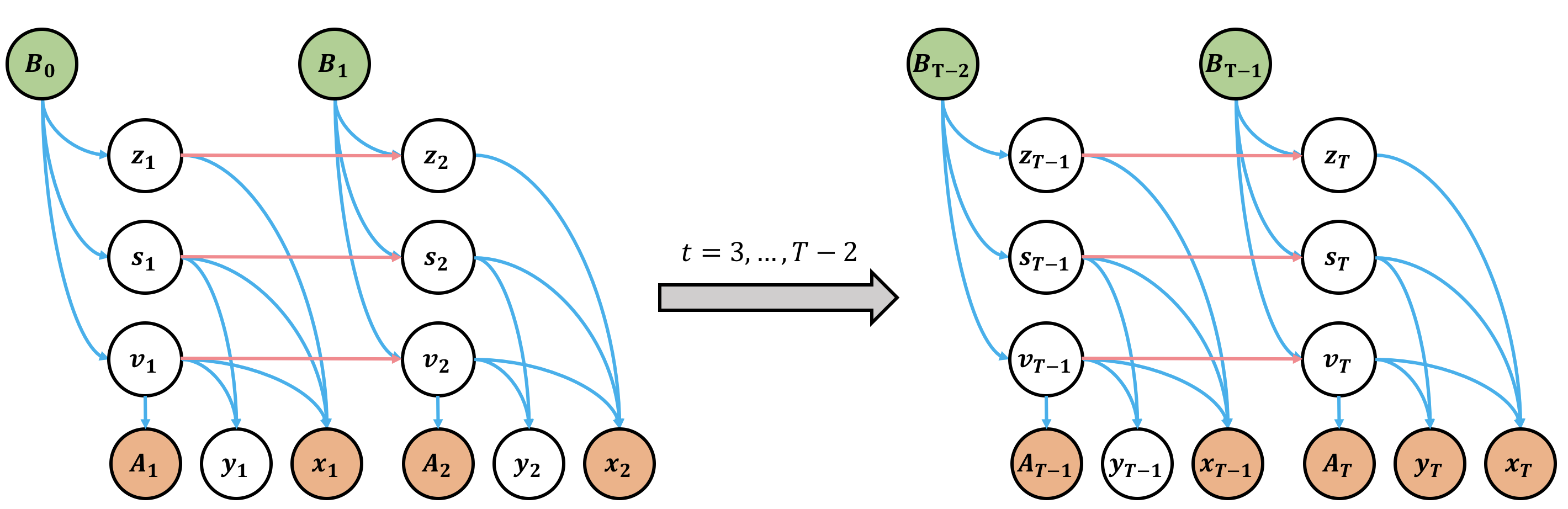
To avoid spurious correlation to enable robust forecasting, we propose Causal Hidden Markov Model (Causal-HMM) in which we explicitly separate the disease-causative features from others, and model them using hidden variables that propagate to generate the medical observation, as encapsulated in the causal graph in Fig. 1. Specifically as shown, among all hidden variables, i.e., that generate the medical image , only are causally related to the disease label . Taking peripapillary atrophy disease [16] as an example, the is related to the clinical measurements that are relevant to the disease (denoted as , e.g., Axial length, Corneal thickness, Corneal curvature) and the is related to other disease-related aspects that beyond clinical measurements but can be reflected in the retinal image (e.g., Maculopathy, Fundus morphology, choroidal vessels). The propagation of these hidden variables are confounded by personal attributes (denoted as such as age, gender, etc.), making the spuriously correlated with the disease and can be learned according to intrinsic bias from observed data. We theoretically show that the hidden variables (i.e., , ) can be possibly identified from observational distribution, benefited from the explicit separation of , and . To the best of our knowledge, we are the first to provide the identifiability result for sequential data in the supervised scenario. For practical inference, we reformulate a new sequential VAE framework that conforms to the causal model above. The disentangled disease-related hidden variables are used for future disease prediction.
We apply our method on an in-house dataset of peripapillary atrophy (PPA) which is related to many irreversible eye diseases. The dataset is divided into training set, validation set and test set with the first two share the same distribution. The empirical results show that compared with other methods, our Causal-HMM can achieve much better prediction accuracy on the out-of-distribution test set, implying the ability to handle spurious correlation of our method. The ablative studies show the effectiveness of each component in our method. The visualization further shows that the identified disease-causative hidden variables by our model are concentrated on the disease-related regions. Our contribution can be summarized as follows:
-
•
Methodologically, we propose a novel Causal Hidden Markov Model of sequential data for future disease forecasting;
-
•
Algorithmically, we reformulate a new sequential VAE framework, which is aligned with the causal model above;
-
•
Theoretically, we provide an identifiability result, which implicitly ensures disentanglement of the disease-causative latent features from others;
-
•
Experimentally, we achieve SOTA prediction result for the peripapillary atrophy forecasting problem, on the out-of-distribution test dataset.
2 Related Work
Conventional methods for disease progression require additional data, which can refer to the supervision signals (e.g., disease labels) at each time step, or target information at the future stage (e.g., image or clinical measurements at future stage), e.g., [13, 21, 11, 26]. Different from them, in our disease forecasting scenario, the target information cannot be observed. Besides, the disease label at each time step is also not provided, which is common in many practical medical scenarios due to large labeling costs.
Other works with more similar settings to ours are modeling sequential or time series data, e.g., [19, 6, 3, 17]. Most of these work implemented Multilayer Perception (MLP) or Convolutional neural networks (CNN) for feature extraction; and use a recurrent neural network (RNN) to generate the trajectory of extracted features, e.g.,[6] and [3]. Instead the [17] proposes to use transformer to capture the long term dependencies. Particularly, the [19] proposed a deep generative model that learned from the low dimensional latent space that assumed to lie on an priori known Riemannian manifold. Specifically, it implemented an RNN to encode the sequential image into hidden embedding and then decoded them to generate the sequential data. However, these models do not separate the features that are causally related to the disease label from others, making them suffer from learning spurious correlation. This spurious correlation inherited from data may not hold on OOD samples, which can cause a high risk for the safety-critical medical data. In contrast, our method explicitly disentangle these disease-causative features (i.e., the hidden variables that are related to the disease) from others, in order to avoid spurious correlation and hence enable the OOD generalization.
There are also works for learning disentanglement of latent space, i.e.,[10, 20]. Specifically, DIVA [10] proposes a generative model by learning three subspaces that account for domain, class and residual variations respectively. COS-CVAE [20] aims to learn context-object split factorization of the latent variables for an image. Different from these work, we model the disentanglement on time series medical images. Besides, we provide an identifiability result together with a reformulated sequential variational auto-encoder, enable the learning of the disease-causative hidden variable (without mixing others).
3 Preliminaries
We provide a brief background of structural causal model (SCM) and one can refer to [22] for more details.
Structural Causal Model. The SCM, according to [22], refers to a causal graph associated with the structural equations. The causal graph is represented by a directed acylic graph (DAG) denoted as with respectively denoting the node set and the edge set. Each arrow in the denotes that the has a direct effect on , i.e., fixing other nodes in except , changing the value of would change the distribution of . The structural equations assign the generating mechanisms of each variable in . Specifically, for , the causal mechanisms associated with the structural equations (defined as ) are defined as: with denoting the set of parent nodes of . The denotes the exogenous variables (i.e., the ones are not of interest/outside the system of the causal graph), which induce the distribution of . According to Causal Markov Condition [22], we have that . The SCM can enable the definition of confounding bias which can induce correlation rather than causation, such as the correlation between and , due to confounder in .
4 Methodology
Problem Setup Notations. Denote respectively as the image, disease status, clinical measurements and personal attributes at time stage . Here the with denoting the disease and denoting the healthy status. We consider the disease progression problem, i.e., with and . To achieve this goal, we observe training data with . Note that we do not require observing for , which agrees with many realistic scenarios in which the labelling can be costly.
Outline. We first introduce our causal hidden Markov Model in section 4.1 in which only a subset of hidden variables are causally related to the disease (i.e., disease-causative features). Then we introduce our method to learn these disease-causative hidden variables in section 4.2. Finally, we in section 4.3 provide an identifiability claim which ensures that such disease-causative features can be disentangled with others.
4.1 Causal Hidden Markov Model
To describe the disease progression, we introduce our causal graph with the DAG illustrated in Fig. 1. As an extension of hidden Markov model to the supervised learning with consideration of disease-causative features, our model is named as Causal Hidden Markov Model (Causal-HMM), which is formally defined as:
Definition 4.1 (Causal-HMM)
To have an intuitive understanding regarding our model, as shown in Fig. 1, we introduce hidden variables to model the latent components of observed variables at time step . These hidden variables, which evolve as the intrinsic drive of the progression of the image and the disease status, are additionally affected by an auxiliary variable (i.e., the personal attributes such as age, gender that characterize the population), as reflected by the arrow in Fig. 1. Such an auxiliary variable can explain the distributional change among populations. Besides, we explicitly separate the hidden variables into three parts: that participant in different generating process. For disease forecasting, the refer to components determining the clinical measurements related to the lesion region of the disease; the denotes additional disease-causative factors that beyond properties but can be reflected in the image; the denotes other concepts that are outside (but can be correlated to) the lesion region. In other words, all these latent variables generate ; but among them, only point to with additionally pointing to . Such a disentanglement of disease-causative hidden variables (i.e., ) from others, is the key to avoid spurious correlation. In the subsequent section, we provide the learning method for the proposed Causal-HMM and our identifiability result which implicitly ensures this disentanglement during learning.
4.2 Learning Method
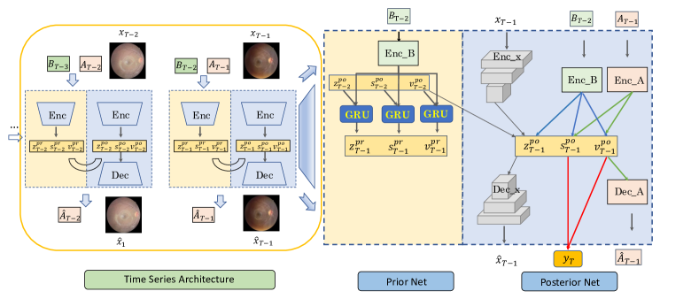
To learn the proposed causal hidden Markov model, we introduce a new reformulated sequential VAE framework based on VAE, with the network architecture shown in Fig. 2. The ELBO with (, for simplicity) as variational distribution is:
| (1) |
where . According to Causal Markov Condition [22], we have the following factorization of joint distribution as:
| (2) |
The ,, are respectively prior models, posteriors models and generative models. Note that the Markov property often exists on disease progression [8, 27] which we also adopt to our learning procedure.
Prior. For the prior , it can be further factorized due to disentanglement of :
| (3) |
where for any , for each is distributed as . The (and ) parameterized by Gated Recurrent Unit (GRU) network [2]. The GRU is to capture the one-step dependency which has been employed in [28]; and following GRU is two FCs with one outputting the mean vector and one outputting the log-variance vector of the hidden variable.
Posterior. Since is expected to mimic the behavior of (also ), it shares the same way of reparameterization with . Under reparameterization with and mean-field factorization222Please refer to supplementary for more details., the posterior is given by:
| (4) |
where .
Specifically, the posterior network is parameterized by a five-layer convolution for encoding image and two fully connected layers for encoding the clinical measurements and personal attributes respectively.
Generations. For each , the generative models , are p.d.f of Gaussian distributions respectively parameterized by composition of deconvolution and that of fully connected (fc) layer, to reconstruct the image and the clinical measurements. The is parameterized as an fc layer followed by softmax classifier. The generation model for image is parameterized by five-layer deconvolution;
Reformulation. Substituting the posterior in Eq. (4.2) and the prior in Eq. (3) in Eq. (1), we reformulate the ELBO as:
| (5) | |||
| (6) | |||
| (7) |
where the are respectively defined as:
Due to the approximation of by , we parameterize the as , with which the degenerates to 0. Besides, we have for :
Training & Test. With such reparameterizations, the reformulated ELBO in Eq. (5) is our maximization objective. During the inference, we iteratively obtain the latent variable at each step via the posterior network . Finally, we feed into the the classifier to predict .
| Methods | RGL [19] | Devised RNN [6] | LogSparse Transformer [17] | Ours | ||||
|---|---|---|---|---|---|---|---|---|
| Grades | ACC | AUC | ACC | AUC | ACC | AUC | ACC | AUC |
| G1 to G5 | 64.70 1.89 | 71.14 1.44 | 74.02 3.82 | 81.75 3.08 | 74.58 4.81 | 79.2 4.69 | 77.19 1.69 | 85.43 1.76 |
| G1 to G4 | 61.46 4.48 | 63.50 5.88 | 66.92 1.06 | 72.88 2.22 | 70.42 4.57 | 73.95 3.98 | 72.89 2.64 | 78.99 1.53 |
| G1 to G3 | 58.33 10.31 | 56.64 5.41 | 63.55 1.47 | 66.45 0.92 | 67.18 1.99 | 70.15 1.1 | 62.43 2.03 | 68.24 2.93 |
| G1 to G2 | 64.17 2.03 | 53.38 4.20 | 57.19 7.45 | 57.07 2.37 | 63.13 4.01 | 65.15 2.12 | 65.42 1.47 | 65.09 2.29 |
| G2 to G5 | 62.29 5.63 | 69.70 5.12 | 73.27 2.44 | 80.16 1.48 | 76.04 0.74 | 84.02 1.76 | 76.26 2.44 | 86.71 0.89 |
| G2 to G4 | 61.25 7.19 | 65.08 5.68 | 67.10 1.79 | 74.21 1.59 | 72.71 2.13 | 80.03 2.19 | 71.22 5.17 | 80.62 1.36 |
| G2 to G3 | 58.12 5.68 | 56.40 4.98 | 63.17 1.94 | 66.87 2.92 | 65.62 4.54 | 67.79 4.49 | 66.91 2.69 | 75.07 1.31 |
| G3 to G5 | 65.62 4.60 | 71.22 5.50 | 74.77 3.03 | 80.57 2.28 | 76.45 4.81 | 83.16 3.56 | 77.01 3.41 | 86.22 1.34 |
| G3 to G4 | 63.54 1.95 | 67.58 3.02 | 68.79 4.46 | 73.49 3.19 | 72.49 4.81 | 77.41 1.99 | 71.77 2.59 | 82.22 1.29 |
| G4 to G5 | 67.29 3.42 | 71.47 3.77 | 75.53 3.07 | 81.81 2.12 | 79.58 2.16 | 86.69 1.52 | 78.13 3.21 | 86.92 1.53 |
| Mean | 62.68 4.72 | 64.41 4.50 | 68.43 3.05 | 73.53 2.22 | 71.82 3.46 | 76.76 2.74 | 71.92 2.73 | 79.55 1.53 |
4.3 Identifiability of Disease-Causative Features
In this section, we provide a theoretical guarantee for our learning method that the disease-causative features at each (a.k.a. ) [25], can be disentangled from others that may encode spurious correlations (a.k.a. ), ensuring the stable learning of our method. Our analysis is inspired but far beyond the recent result [14] in nonlinear ICA to the supervised learning with time-series graphical model, in which the main objective is to disentangle the from at each time step in order to avoid spurious correlation. Similar to [14, 15], we assume the are generated by Additive Noise Model (ANM), which can be a wide class of continuous and categorical distributions [12]. Besides, we assume that the latent variables for every ) belong to the exponential family:
for any . Here the denote the sufficient statistics and natural parameters; and the denote the base measures and normalizing constants to ensure the integral of distribution equals to 1. Let and . Then we have the following identifiability result for :
Theorem 4.2 (Identifiability)
We assume that are bijective. Denote . Under the following conditions:
-
•
are differentiable and non-zero almost everywhere for any and .
-
•
For every , there exists at least with and values of , i.e., such that the have full column rank and ,
we have that if and give rise to the same observational distribution, i.e., for any and , then there exists invertible matrices and vectors such that:
| (8) | |||
| (9) | |||
| (10) | |||
| (11) |
Remark 1
The is related to . The second “full-column” rank condition, as an indication of independence of natural parameters , implies that the distributions with different personal attributes (population) are diverse enough, which is also assumed in [14].
Note that the Eq. (8), (9), (10) imply the disentanglement of unless the extreme case that these three latent components can be represented by each other, i.e., there exists such that or . Besides, the Eq. (11) shows that we can learn the same prediction at time to the ground-truth (consider the as the ground-truth oracle parameter and the denotes or learned parameter), under the deterministic setting (i.e., ). Such an identifiability result ensures the disentanglement of our method. Besides, it does not contradict with the conclusion in [18] of “impossibility to learn disentangled representations without supervision”, since our learning is additionally supervised by the label , the clinical measurements and also guided by the personal attributes as side information.
5 Experiments and Analysis
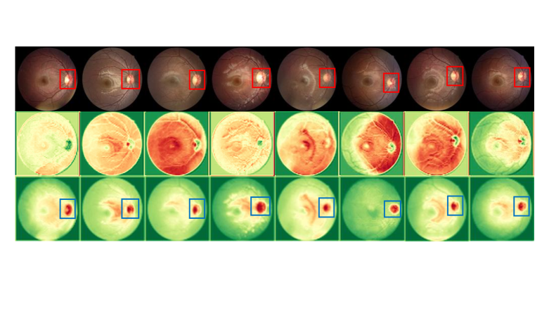
In this section, we apply our method on in-house data that studies the peripapillary atrophy (PPA) development among primary school students. The atrophy happens around the region of the optic disc (as marked by the red rectangle in Fig. 3). Since the PPA can cause irreversible myopia retinas in children, the forecast of it at an early stage is extremely valuable to slow down the progression.
5.1 Dataset
| Methods | CNN | CNN+LSTM | Seq VAE | Seq VAE + Att | Ours | |||||
|---|---|---|---|---|---|---|---|---|---|---|
| Grades | ACC | AUC | ACC | AUC | ACC | AUC | ACC | AUC | ACC | AUC |
| G1 to G5 | 62.17 3.97 | 65.01 1.48 | 74.39 1.56 | 80.25 1.93 | 75.40 1.08 | 81.67 1.66 | 74.21 4.79 | 84.46 1.54 | 77.19 1.69 | 85.43 1.76 |
| G1 to G4 | 61.64 1.04 | 60.99 2.42 | 69.36 2.91 | 72.39 3.16 | 68.78 4.10 | 73.50 1.99 | 71.21 2.75 | 76.68 2.08 | 72.89 2.64 | 78.99 1.53 |
| G1 to G3 | 58.07 3.75 | 56.75 1.99 | 61.31 1.42 | 65.48 2.23 | 60.75 1.93 | 67.05 2.75 | 60.78 0.93 | 61.34 0.91 | 62.43 2.03 | 68.24 2.93 |
| G1 to G2 | 59.25 1.56 | 55.74 1.76 | 59.44 3.94 | 58.45 3.21 | 62.62 0.00 | 58.00 1.62 | 62.43 0.42 | 59.56 4.79 | 65.42 1.47 | 65.09 2.29 |
| G2 to G5 | 64.11 2.83 | 66.65 1.14 | 70.84 1.92 | 79.09 1.15 | 72.52 1.08 | 81.16 0.91 | 77.19 5.14 | 84.88 1.17 | 76.26 2.44 | 86.71 0.89 |
| G2 to G4 | 61.23 4.01 | 64.67 1.25 | 69.34 1.67 | 72.68 1.56 | 68.85 1.32 | 73.69 1.75 | 74.39 3.14 | 77.66 0.99 | 71.22 5.17 | 80.62 1.36 |
| G2 to G3 | 59.25 1.97 | 62.82 2.07 | 61.49 1.92 | 66.67 2.74 | 64.02 3.77 | 61.91 3.08 | 61.31 0.84 | 62.63 3.46 | 66.91 2.69 | 75.07 1.31 |
| G3 to G5 | 67.35 2.75 | 71.20 1.61 | 74.21 2.52 | 80.35 1.28 | 74.53 1.06 | 80.71 1.96 | 76.63 3.43 | 84.42 1.80 | 77.01 3.41 | 86.22 1.34 |
| G3 to G4 | 62.89 3.02 | 68.25 2.98 | 68.59 4.11 | 71.96 6.56 | 67.29 2.29 | 74.58 0.85 | 74.77 0.93 | 79.24 0.99 | 71.77 2.59 | 82.22 1.29 |
| G4 to G5 | 70.75 3.96 | 77.58 1.37 | 75.51 3.93 | 82.42 2.51 | 73.83 3.58 | 79.65 1.65 | 76.45 2.91 | 84.45 0.48 | 78.13 3.21 | 86.92 1.53 |
| Mean | 62.67 2.89 | 64.97 1.81 | 68.45 2.59 | 72.97 2.63 | 68.86 2.02 | 73.19 1.82 | 70.94 2.53 | 75.53 1.82 | 71.92 2.73 | 79.55 1.62 |
| Variables | + | |||||||||||
|---|---|---|---|---|---|---|---|---|---|---|---|---|
| Dataset | Training | Validation | Test | Training | Validation | Test | ||||||
| Grades | ACC | AUC | ACC | AUC | ACC | AUC | ACC | AUC | ACC | AUC | ACC | AUC |
| G1 to G5 | 94.72 1.96 | 99.40 0.36 | 72.20 1.10 | 75.10 0.18 | 78.88 1.06 | 83.75 0.29 | 99.93 0.16 | 100.00 0.00 | 71.20 1.64 | 78.10 0.24 | 67.10 1.22 | 68.98 0.45 |
| G1 to G4 | 98.88 1.81 | 99.86 0.30 | 64.40 1.34 | 66.06 0.42 | 70.09 0.66 | 70.55 0.57 | 79.51 6.79 | 87.94 5.44 | 59.40 3.29 | 60.96 0.47 | 60.75 1.14 | 63.32 1.69 |
| G1 to G3 | 79.51 4.24 | 86.88 3.76 | 59.20 4.91 | 60.17 0.55 | 59.81 3.67 | 64.09 0.87 | 58.68 1.67 | 52.79 3.89 | 63.00 0.71 | 55.42 1.48 | 61.68 0.66 | 42.37 0.66 |
| G1 to G2 | 69.51 1.64 | 74.30 1.25 | 70.80 3.56 | 63.46 0.64 | 69.16 2.64 | 70.43 0.47 | 79.65 2.97 | 88.70 3.28 | 65.40 2.97 | 61.83 0.53 | 53.83 1.82 | 48.79 1.41 |
| G2 to G5 | 98.13 2.49 | 99.84 0.33 | 74.40 1.14 | 75.23 0.09 | 78.13 1.42 | 83.92 0.21 | 100.00 0.00 | 100.00 0.00 | 70.60 0.55 | 77.84 0.47 | 66.92 0.51 | 68.65 0.20 |
| G2 to G4 | 97.78 2.03 | 99.54 0.81 | 63.40 2.23 | 65.99 0.38 | 70.47 1.94 | 71.18 0.91 | 85.83 4.88 | 92.69 4.29 | 58.60 1.95 | 60.82 0.97 | 60.75 1.48 | 61.86 0.56 |
| G2 to G3 | 77.15 4.93 | 84.31 5.19 | 64.40 1.67 | 61.20 0.78 | 64.30 2.03 | 64.69 2.31 | 56.81 2.05 | 49.24 0.59 | 63.00 0.00 | 54.47 1.71 | 62.63 0.78 | 43.93 2.06 |
| G3 to G5 | 96.81 1.38 | 99.78 0.16 | 74.00 2.12 | 75.42 0.37 | 77.94 1.94 | 83.83 0.30 | 100.00 0.00 | 100.00 0.00 | 70.60 0.89 | 77.43 0.28 | 66.17 1.02 | 68.92 0.23 |
| G3 to G4 | 99.10 0.76 | 99.94 0.08 | 64.40 1.52 | 68.04 0.82 | 68.04 1.79 | 72.51 0.51 | 85.49 8.17 | 92.21 5.74 | 60.80 1.30 | 61.38 0.98 | 60.75 2.19 | 62.24 2.19 |
| G4 to G5 | 95.07 2.28 | 99.52 0.42 | 72.20 1.30 | 74.97 0.18 | 78.13 1.06 | 83.71 0.11 | 99.38 0.86 | 99.97 0.05 | 70.40 0.55 | 77.31 0.34 | 67.66 2.52 | 67.46 0.46 |
| Mean | 90.67 2.35 | 94.34 1.27 | 67.94 2.09 | 68.56 0.44 | 71.50 1.82 | 74.87 0.66 | 84.53 2.76 | 86.35 2.33 | 65.30 1.39 | 66.56 0.75 | 62.82 1.33 | 59.65 0.99 |
Our data contains 507 sequential data, i.e., retinal images, clinical measurements and personal attributes of 507 students in primary school from the 1st grade to the 6th grade. Only the disease label at the 6th grade (i.e., ) are provided with being (healthy) for all samples. The respectively denote the retinal image, clinical measurements related to the PPA, the personal attributes and the disease label. Our goal is to predict the disease label at the 6th grade (i.e., the ), given with . To validate the effectiveness of our method on handling OOD data, the sex ratio which has been found significantly correlated with disease progression [4, 29], is different between the test data (boy/girl: 3/1) and the training, validation data (boy/girl: 2/3). After this splitting, the training, validation and test set contain 300, 100 and 107 samples, respectively. The clinical measurements are represented by 15 vision-related attributes; while the personal attributes are represented by 16 attributes 333please refer to supplementary information for details..
Gender v.s. Disease. We conduct a Bilateral T-test of whether gender affects the disease. We assume the disease rate of boys and girls are respectively binomial distributions with parameters , denoted as and . The and hypothesis are: . The calculated -value in our dataset is 0.03876, implying that the probability of making an error if we admit (denying ) is less than . Therefore, the datasets with different sex ratios can have the distributional difference, verifying that the distributions of training set and test set are different.
5.2 Quantitative Results
For comparison, we compare with the following methods. 1) RGL [19] shares the most similar scenario with ours. They proposes to predict the disease progression by learning a Riemannian manifold space. To compare fairly, we additionally append a classifier after the latent space for disease prediction. 2) Devised RNN [6] employs deep convolutional neural network and recurrent neural network to learn longitudinal features for disease classification. We also provide the attributes for its learning when adopting this method to our problem. 3) LogSparse Transformer [17] is a transformer-based method for time series forecasting. Similarly, to compare fairly, we additionally append a classifier after the transformer network.
The prediction accuracy (ACC) and Area Under the ROC curve (AUC) are measured for evaluation. We consider time series settings for possible pairs of (e.g., the “G1 to G5” means ). All results are shown in Tab. 1. As shown, our method achieves better result on both ACC and AUC than the compared baselines on almost all settings and the average setting. When comparing different settings inside one method, we see that using data more closer to the future stage leads to higher performance, showing that the closer stage contains more useful information for future disease. Note that looking further into the past does not boost the performance, we point that this is due to the current image has contained the sufficient information for future disease. What we should do on this sequential data is to prompt the future prediction by making use of the past time dependency. To compare in all settings, Devised RNN [6] performs better than RGL [19] benefiting from attribute data. The LogSparse Transformer [17] outperforms the first two due to the higher ability for learning time dependencies. While they are all weaker than ours. Especially ours outperforms the RGL [19] by a large margin. Since such a latent space in RGL is for generating the whole image for disease prediction, it can mix the correlated by non-causative features of the disease. Devised RNN [6] and LogSparse Transformer [17] also face the same problem.
5.3 Ablation Study
In this section, we give a more comprehensive analysis regarding the effectiveness of the sequential modeling, clinical measurements provided as side information to help identification of latent space, and especially disentanglement of disease-causative hidden variables in handling OOD generalization. The compared variants are:
Vanilla CNN. Directly implement vanilla CNNs on images that share the same network structure with our encoder, and then we append two fully connected layers for prediction. The model does not make use of the time dependency between sequential data.
CNN+LSTM. We incorporate CNN into Long Short-Term Memory networks (LSTMs) [9] to extract the features on sequential image data; then similarly, we use two fully connected layers for prediction.
Seq VAE. We implement sequential variational autoencoder framework that shares the same time series architecture as ours. What’s the difference from our method is that the clinical measurements and personal attributes are not provided and there is no disentanglement.
Seq VAE + Att. The baseline is the same to ours only without separation of , to validate the advantage of disentanglement of disease-causative hidden variables from others.
Results. As shown in Tab. 2, the implementation of our time series model can achieve better results, showing the improvement of Seq VAE over Vanilla CNN and CNN+LSTM. The performance is further improved by leveraging the information of attributes (as shown by the improvement of Seq VAE + Att over Seq VAE). This improvement comes from two-fold contributions of attributes: i) the observation of clinical measurements that help identify the latent variable ; and ii) the personal attributes provided as auxiliary variables for learning the hidden variables. Finally, the improvement of Ours over Seq VAE + Att can validate the effectiveness of separating our disease-causative hidden variables in order to avoid spurious correlation.
Robustness due to Disentanglement. To further valid the benefit regarding the robustness of disease-causative hidden variables over others, we implement a two-step tuning method for and . Specifically, after training the whole model at the first stage, we obtain the disease-unrelated hidden variable and the disease-related hidden variables and . We additionally train a classifier to predict the disease respectively by and , i.e., and . As shown in Tab. 3, the suffers from a significant performance drop from validation to test however the remains robust across validation and test. This can validate the existence of redundant variables that are spuriously correlated to the disease and can be learned during the data-fitting process. Separating these variables out during training can help avoid spurious correlation and therefore achieve more robustness on OOD samples.
5.4 Visualization
We visualize the high-response region for learned and . Specifically, we implement Grad-CAM (Gradient-weighted Class Activation Mapping [23]) to compute the feature map matrix by performing backpropagation on and . The visualized feature maps are shown in Fig. 3, with the top row, the middle row, and the bottom row representing the original images, the visualized feature maps for and . From red to green correspond to high to low response value. As shown, the high response area for is concentrated to the optic disc as marked by blue rectangles, which was to be highly correlated to the disease status [16, 5]. In contrast, the high-response area for is scattered distributed into other areas such as macular. Due to data bias, the can be spuriously correlated with the disease, however cannot generalize to other distributions.
6 Conclusion and Future Work
We propose a causal Hidden Markov Model for forecasting the disease at the future stage, given data up to the current stage. To enable OOD generalization on medical data that can suffer from a distributional change among populations, we propose to explicitly separate the disease-causative factors from others. Under the identifiable result that ensures the disentanglement of such disease-related hidden variables, we reformulate a new sequential VAE that conforms to our causal model for practical inference. The experimental results and the follow-up analysis validate the effectiveness and robustness of our model. The application of our method on more broad scenarios (such as Alzheimer’s Disease) is left in our future work.
7 Acknowledgements
This work was supported by MOST-2018AAA0102004, NSFC-61625201 and NSFC-62061136001.
References
- [1] Brittany J Carr and William K Stell. The science behind myopia. In Webvision: The Organization of the Retina and Visual System [Internet]. University of Utah Health Sciences Center, 2017.
- [2] Junyoung Chung, Caglar Gulcehre, KyungHyun Cho, and Yoshua Bengio. Empirical evaluation of gated recurrent neural networks on sequence modeling. arXiv preprint arXiv:1412.3555, 2014.
- [3] R. Cui, M. Liu, and G. Li. Longitudinal analysis for alzheimer’s disease diagnosis using rnn. In 2018 IEEE 15th International Symposium on Biomedical Imaging (ISBI 2018), pages 1398–1401, 2018.
- [4] Maciej Czepita, Damian Czepita, and Krzysztof Safranow. Role of gender in the prevalence of myopia among polish schoolchildren. Journal of ophthalmology, 2019.
- [5] Savatovsky E, Mwanza JC, Budenz DL, Feuer WJ, Vandenbroucke R, Schiffman JC, and Anderson DR. Longitudinal changes in peripapillary atrophy in the ocular hypertension treatment study: a case-control assessment. Ophthalmology, 122(1):79–86, 01 2015.
- [6] Linlin Gao, Haiwei Pan, Fujun Liu, Xiaoqin Xie, Zhiqiang Zhang, and Jinming Han. Brain disease diagnosis using deep learning features from longitudinal mr images. In APWeb/WAIM, 2018.
- [7] Ian J Goodfellow, Jonathon Shlens, and Christian Szegedy. Explaining and harnessing adversarial examples. arXiv preprint arXiv:1412.6572, 2014.
- [8] Chantal Guihenneuc-jouyaux, Sylvia Richardson, and Ira Longini. Modelling markers of disease progression by a hidden markov process: application to characterising cd4 cell decline. 07 2000.
- [9] Sepp Hochreiter and Jürgen Schmidhuber. Long short-term memory. Neural computation, 9(8):1735–1780, 1997.
- [10] Maximilian Ilse, Jakub M Tomczak, Christos Louizos, and Max Welling. Diva: Domain invariant variational autoencoders. In Medical Imaging with Deep Learning, pages 322–348. PMLR, 2020.
- [11] Jiang J, Liu X, Liu L, and et al. Predicting the progression of ophthalmic disease based on slit-lamp images using a deep temporal sequence network. PLoS One, 2018.
- [12] D Janzing, J Peters, JM Mooij, and B Schölkopf. Identifying confounders using additive noise models. In Proceedings of the 25th Conference on Uncertainty in Artificial Intelligence (UAI 2009), pages 249–257. AUAI Press, 2009.
- [13] B. Jie, M. Liu, J. Liu, D. Zhang, and D. Shen. Temporally constrained group sparse learning for longitudinal data analysis in alzheimer’s disease. IEEE Transactions on Biomedical Engineering, 64(1):238–249, 2017.
- [14] Ilyes Khemakhem, Diederik P Kingma, and Aapo Hyvärinen. Variational autoencoders and nonlinear ICA: A unifying framework. In Proceedings of the 23th International Conference on Artificial Intelligence and Statistics (AISTATS-23), volume 108, Palermo, Italy, 2020. AISTATS Committee, PMLR.
- [15] Ilyes Khemakhem, Ricardo Pio Monti, Diederik P Kingma, and Aapo Hyvärinen. Ice-beem: Identifiable conditional energy-based deep models. arXiv preprint arXiv:2002.11537, 2020.
- [16] Sun Young Kim, Hae-Young L. Park, and Chan Kee Park. The Effects of Peripapillary Atrophy on the Diagnostic Ability of Stratus and Cirrus OCT in the Analysis of Optic Nerve Head Parameters and Disc Size. Investigative Ophthalmology and Visual Science, 53(8):4475–4484, 07 2012.
- [17] Shiyang Li, Xiaoyong Jin, Yao Xuan, Xiyou Zhou, Wenhu Chen, Yu-Xiang Wang, and Xifeng Yan. Enhancing the locality and breaking the memory bottleneck of transformer on time series forecasting. In Advances in Neural Information Processing Systems, pages 5243–5253, 2019.
- [18] Francesco Locatello, Stefan Bauer, Mario Lucic, Gunnar Raetsch, Sylvain Gelly, Bernhard Schölkopf, and Olivier Bachem. Challenging common assumptions in the unsupervised learning of disentangled representations. In International Conference on Machine Learning, pages 4114–4124, 2019.
- [19] Maxime Louis, Raphael Couronne, Igor Koval, Benjamin Charlier, and Stanley Durrleman. Riemannian geometry learning for disease progression modelling. In International Conference on Information Processing in Medical Imaging, pages 542–553. Springer, 2019.
- [20] Shweta Mahajan and Stefan Roth. Diverse image captioning with context-object split latent spaces. arXiv preprint arXiv:2011.00966, 2020.
- [21] Zhenyuan Ning, Yu Zhang, Yongsheng Pan, Tao Zhong, Mingxia Liu, and Dinggang Shen. Ldgan: Longitudinal-diagnostic generative adversarial network for disease progression prediction with missing structural mri. In International Workshop on Machine Learning in Medical Imaging, pages 170–179. Springer, 2020.
- [22] Judea Pearl. Causality. Cambridge university press, 2009.
- [23] Ramprasaath R. Selvaraju, Abhishek Das, Ramakrishna Vedantam, Michael Cogswell, Devi Parikh, and Dhruv Batra. Grad-cam: Why did you say that? visual explanations from deep networks via gradient-based localization. CoRR, abs/1610.02391, 2016.
- [24] Xinwei Sun, Lingjing Hu, Yuan Yao, and Yizhou Wang. Gsplit lbi: Taming the procedural bias in neuroimaging for disease prediction. In International Conference on Medical Image Computing and Computer-Assisted Intervention, pages 107–115. Springer, 2017.
- [25] Xinwei Sun, Botong Wu, Chang Liu, Xiangyu Zheng, Wei Chen, Tao Qin, and Tie-yan Liu. Latent causal invariant model. arXiv preprint arXiv:2011.02203, 2020.
- [26] Sarah J Tabrizi, Rachael I Scahill, Alexandra Durr, Raymund AC Roos, Blair R Leavitt, Rebecca Jones, G Bernhard Landwehrmeyer, Nick C Fox, Hans Johnson, Stephen L Hicks, Christopher Kennard, David Craufurd, Chris Frost, Douglas R Langbehn, Ralf Reilmann, and Julie C Stout. Biological and clinical changes in premanifest and early stage huntington’s disease in the track-hd study: the 12-month longitudinal analysis. The Lancet Neurology, 10(1):31 – 42, 2011.
- [27] Liu YY, Ishikawa H, Chen M, Wollstein G, Schumnan JS, and Rehg JM. Longitudinal modeling of glaucoma progression using 2-dimensional continuous-time hidden markov model. page 444–451, 2013.
- [28] Shuai Zheng et al. Conditional random fields as recurrent neural networks. In ICCV, pages 5243–5253, 2015.
- [29] Wen-Jun Zhou, Yong-Ye Zhang, Hua Li, Yu-Fei Wu, Ji Xu, Sha Lv, Ge Li, Shi-Chun Liu, and Sheng-Fang Song. Five-year progression of refractive errors and incidence of myopia in school-aged children in western china. Journal of epidemiology, page JE20140258, 2016.