Scheduling in the Secretary Model

Abstract

This paper studies Makespan Minimization in the random-order model. Formally, jobs, specified by their processing times, are presented in a uniformly random order. An online algorithm has to assign each job permanently and irrevocably to one of $m$ parallel and identical machines such that the expected time it takes to process them all, the makespan, is minimized.

We give two deterministic algorithms. First, a straightforward adaptation of the semi-online strategy $\mathrm{LightLoad}$ [3] provides a very simple algorithm retaining its competitive ratio of $1.75$. A new and sophisticated algorithm is $1.535$-competitive. These competitive ratios are not only obtained in expectation but, in fact, for all but a very tiny fraction of job orders.

Classically, online makespan minimization only considers the worst-case order. Here, no competitive ratio below $1.885$ for deterministic algorithms and $1.581$ using randomization is possible. The best randomized algorithm so far is $1.916$-competitive. Our results show that classical worst-case orders are quite rare and pessimistic for many applications. They also demonstrate the power of randomization when compared much stronger deterministic reordering models.

We complement our results by providing first lower bounds. A competitive ratio obtained on nearly all possible job orders must be at least $1.257$. This implies a lower bound of $1.043$ for both deterministic and randomized algorithms in the general model.

1 Introduction

We study one of the most basic scheduling problems, the classic problem of makespan minimization. For the classic makespan minimization problem one is given an input set $\mathcal{J}$ of $n$ jobs, which have to be scheduled onto $m$ identical and parallel machines. Preemption is not allowed. Each job $J\in\mathcal{J}$ runs on precisely one machine. The goal is to find a schedule minimizing the makespan, i.e. the last completion time of a job. This problem admits a long line of research and countless practical applications in both, its offline variant see e.g. [29, 31] and references therein, as well as in the online setting studied in this paper.

In the online setting jobs are revealed one by one and each has to be scheduled by an online algorithm $A$ immediately and irrevocably without knowing the sizes of future jobs. The makespan of online algorithm $A$, denoted by $A(\mathcal{J}^{\sigma})$, may depend on both the job set $\mathcal{J}$ and the job order $\sigma$. The optimum makespan ${\mathrm{OPT}}(\mathcal{J})$ only depends on the former. Traditionally, one measures the performance of $A$ in terms of competitive analysis. The input set $\mathcal{J}$ as well as the job order $\sigma$ are chosen by an adversary whose goal is to maximize the ratio $\frac{A(\mathcal{J}^{\sigma})}{{\mathrm{OPT}}(\mathcal{J})}$. The maximum ratio, $c=\sup_{\mathcal{J},\sigma}\frac{A(\mathcal{J}^{\sigma})}{{\mathrm{OPT}}(\mathcal{J})}$, is the (adversarial) competitive ratio. The goal is to find online algorithms obtaining small competitive ratios.

In the classical secretary problem the goal is to hire the best secretary out of a linearly ordered set $S$ of candidates. Its size $n$ is known. Secretaries appear one by one in a uniformly random order. An online algorithm can only compare secretaries it has seen so far. It has to decide irrevocably for each new arrival whether this is the single one it wants to hire. Once a candidate is hired, future ones are automatically rejected even if they are better. The algorithm fails unless it picks the best secretary. Similar to makespan minimization this problem has been long studied, see [19, 22, 23, 32, 41, 43, 44] and references therein.

This paper studies a makespan minimization under the input model of the secretary problem. The adversary determines a job set of known size $n$. Similar to the secretary problem, these jobs are presented to an online algorithm $A$ one by one in a uniformly random order. Again, $A$ has to schedule each job without knowledge of the future. The expected makespan is considered. The competitive ratio in the secretary (or random-order) model $c=\sup_{\mathcal{J}}\mathbf{E}_{\sigma}\left[\frac{A(\mathcal{J}^{\sigma})}{{\mathrm{OPT}}(\mathcal{J})}\right]$ is the maximum ratio between the expected makespan of $A$ and the optimum makespan. The goal is again to obtain small competitive ratios.

We propose the term secretary model, first used in [48], to set this model apart from the model studied by the same authors in [5] where $n$, the number of jobs, is not known in advance. Not knowing $n$ is quite restrictive and has never been considered in any other work on scheduling with random-order arrival [26, 48, 49]. For the adversarial model such information is useless.

Similar frameworks received a lot of recent attention in the research community sparking the area of random-order analysis. Random-order analysis has been successfully applied to numerous problems such as matching [27, 33, 35, 45], various generalizations of the secretary problem [7, 22, 23, 32, 41, 43], knapsack problems [8], bin packing [39], facility location [46], packing LPs [40], convex optimization [30], welfare maximization [42], budgeted allocation [47] and recently scheduling [5, 26, 48, 49].

For makespan minimization the role of randomization is poorly understood. The lower bound of $1.581$ from [11, 51] is considered pessimistic and exhibits quite a big gap towards the best randomized ratio of $1.916$ from [2].

The upper bound of $1.535$ in this paper demonstrates surprising power when it comes to randomization in the input order. The power of reordering has been studied by Englert et. al. [20]. Their lower bound considers online algorithms, which are able to look-ahead and rearrange almost all of the input sequence in advance. Their only disadvantage is that such rearrangement is deterministic. Englert et. al.  show that these algorithms can not be better than $1.466$-competitive for general $m$. This is quite close to our upper bound of $1.535$, given that the algorithm involved has neither look-ahead nor control over the arrangement of the sequence.

A main consequence of the paper is that random-order arrival allows to beat the lower bound of $1.581$ for randomized adversarial algorithms. This formally sets this model apart from the classical adversarial setting even if randomization is involved.

Previous work:

Online makespan minimization and variants of the secretary problem have been studied extensively. We only review results most relevant to this work beginning with the traditional adversarial setting. For $m$ identical machines, Graham [29] showed 1966 that the greedy strategy, which schedules each job onto a least loaded machine, is $\left(2-\frac{1}{m}\right)$-competitive. This was subsequently improved in a long line of research [25, 9, 34, 1] leading to the currently best competitive ratio by Fleischer and Wahl [24], which approaches $1.9201$ for $m\rightarrow\infty$. Chen et al. [12] presented an algorithm whose competitive ratio is at most $(1+\varepsilon)$-times the optimum one, though the actual ratio remains to be determined. For general $m$, lower bounds are provided in [21, 10, 28, 50]. The currently best bound is due to Rudin III [50] who shows that no deterministic online algorithm can be better than $1.88$-competitive.

The role of randomization in this model is not well understood. The currently best randomized ratio of $1.916$ [2] barely beats deterministic guarantees. In contrast, the best lower bound approaches $\frac{e}{e-1}>1.581$ for $m\rightarrow\infty$ [11, 51]. There has been considerable research interest in tightening the gap.

Recent results for makespan minimization consider variants where the online algorithm obtains extra resources. There is the semi-online setting where additional information on the job sequence is given in advance, like the optimum makespan [36] or the total processing time of jobs [3, 13, 38, 37]. In the former model the optimum competitive ratio lies in the interval $[1.333,1.5]$, see [36], while for the latter the optimum competitive ratio is known to be $1.585$ [3, 37]. Taking this further, the advice complexity setting allows the algorithm to receive a certain number of advice bits from an offline oracle [4, 18, 38].

The work of Englert et. al. [20] is particularly relevant as they, too, study the power of reordering. Their algorithm has a buffer, which can reorder the sequence ’on the fly’. They prove that a buffer size linear in $m$ suffices to be $1.466$-competitive. Their lower bound shows that this result cannot be improved for any sensible buffer size.

The secretary problem is even older than scheduling [23]. Since the literature is vast, we only summarize the work most relevant to this paper. Lindley [44] and Dynkin [19] first show that the optimum strategy finds the best secretary with probability $1/e$ for $n\rightarrow\infty$. Recent research focusses on many variants, among others generalizations to several secretaries [6, 41] or even matroids [7, 22, 43]. A modern version considers adversarial orders but allows prior sampling [15, 32]. Related models are prophet inequalities and the game of googol [14, 16].

So far, little is known for scheduling in the secretary model. Osborn and Torng [49] prove that Graham’s greedy strategy is still not better than $2$-competitive for $m\rightarrow\infty$. In [5] we studied the very restricted variant where $n$, the number of jobs, is not known in advance and provide a $1.8478$-competitive algorithm and first lower bounds. Here, most common techniques, e.g. sampling, do not work. We are the only ones who ever considered this restriction. Molinary [48] studies a very general scheduling problem. His algorithm has expected makespan $(1+\varepsilon){\mathrm{OPT}}+O(\log(m)/\varepsilon)$, but its random-order competitive ratio is not further analyzed. Göbel et al. [26] study a scheduling problem on a single machine where the goal is to minimize weighted completion times. Their competitive ratio is $O(\log(n))$ whereas they show that the adversarial model allows no sublinear competitive ratio.

Our contribution:

We study makespan minimization for the secretary (or random-order) model in depth. We show that basic sampling ideas allow to adapt a fairly simple algorithm from the literature [3] to be $1.75$-competitive. A more sophisticated algorithm vastly improves this competitive ratio to $1.535$. This beats all lower bounds for adversarial scheduling, including the bound of $1.582$ for randomized algorithms.

Our main results focus on a large number of machines, $m\rightarrow\infty$. This is in line with most recent adversarial results [2, 24] and all random-order scheduling results [5, 26, 48, 49]. While adversarial guarantees are known to improve for small numbers of machines, nobody has ever, to the best of our knowledge, explored guarantees for random-order arrival on a small number of machines. We prove that our simple algorithm is $\left(1.75+O\left(\frac{1}{\sqrt{m}}\right)\right)$-competitive. Explicit bounds on the hidden term are given as well as simulations, which indicate good performance in practice. This shows that the focus of contemporary analyses on the limit case is sensible and does not hide unreasonably large additional terms.

All results in this paper abide to the stronger measure of nearly competitiveness from [5]. An algorithm is required to achieve its competitive ratio not only in expectation but on nearly all input permutations. Thus, input sequences where it is not obtained can be considered extremely rare and pathological. Moreover, we require worst-case guarantees even for such pathological inputs. This seems quite relevant to practical applications, where we do not expect fully random inputs. Both algorithms in this paper hold up to this stronger measure of nearly competitiveness.

A basic approch in random-order models relies on sampling; a small part of the input is used to predict the rest. Sampling allows us to include techniques from semi-online and advice scheduling with two further challenges. On the one hand, the advice is imperfect and may be, albeit with low probability, totally wrong. On the other hand, the advice has to be learned, rather than being available right from the start. In the beginning ’mistakes’ cannot be avoided. This makes it impossible to adapt better semi-online algorithms than $\mathrm{LightLoad}$, namely [13, 38, 37] to our model. These algorithms need to know the total processing volume right from the start. Note that the advanced algorithm in this paper out-competes the optimum competitive ratio of $1.585$ these semi-online algorithms can achieve [1, 37]. We conjecture that this is not possible for algorithms that solely use sampling.

Algorithms that can only use sampling are studied in a modern variant of the secretary problem [15, 32]. First, a random sample is observed, then the sequence is treated in adversarial order. The analysis of $\mathrm{LightLoad}$ carries over to such a model without changes. The $1.535$-competitive algorithm does not maintain its competitive ratio in such a model.

The $1.535$-competitive main algorithm is based on a modern point of view, which, analogous to kernelization, reduces complex inputs to sets of critical jobs. A set of critical jobs is estimated using sampling. Critical jobs impose a lower bound on the optimum makespan. If the bound is high, an enhanced version of Graham’s greedy strategy suffices; called the Least-Loaded-Strategy. Else, it is important to schedule critical jobs correctly. The Critical-Job-Strategy, based on sampling, estimates the critical jobs and schedules them ahead of time. An easy heuristic suffices, due to uncertainty involved in the estimates. Uncertainty poses not only the main challenge in the design of the Critical-Job-Strategy. On a larger scale, it also makes it hard to decide, which of the two strategies to use. Sometimes the Critical-Job-Strategy is chosen wrongly. These cases comprise the crux of the analysis and require using random-order arrival in a novel way beyond sampling.

The analyses of both algorithms follows three steps. First, adversarial analyses give worst-case guarantees and take care of simple job sets, which lack structure to be exploited via random reordering. Intuitively, random sequences have certain properties, like being not ’ordered’. A second step formalizes this, introducing stable orders. Non-stable orders are rare and negligible. Reducing to stable orders yields a natural semi-online setting. Third, we analyze our algorithm in this semi-online setting. See Figure 3 for a lay of the land.

The paper concludes with lower bounds for the secretary model. No algorithm, deterministic or randomized, is better than nearly $1.257$-competitive. This immediately yields a lower bound of $1.043$ in the general secretary model, too.

2 Notation

Almost all notations relevant in scheduling depend on the input set $\mathcal{J}$ or on the ordered input sequence $\mathcal{J}^{\sigma}$. We use the notation $[\mathcal{J}]$ and $[\mathcal{J}^{\sigma}]$ to indicate such dependency, for example $L[\mathcal{J}]$ and $L_{\varphi}[\mathcal{J}^{\sigma}]$. If such dependency needs not be mentioned, for example if the sequence $\mathcal{J}^{\sigma}$ is fixed, we drop this appendage, simply writing $L$ and $L_{\varphi}$. Similarly, we write ${\mathrm{OPT}}$ for ${\mathrm{OPT}}(\mathcal{J})$. If we focus on the job order $\sigma$ whilst the dependency of the job set $\mathcal{J}$ does not deserve mention, the notation $[\sigma]$ instead of $[\mathcal{J}^{\sigma}]$ is used. We could for example write $L_{\varphi}[\sigma]$.

3 A strong measure of random-order competitiveness

Consider a set of $n$ jobs $\mathcal{J}=\{J_{1},\ldots,J_{n}\}$ with non-negative sizes $p_{1},\ldots,p_{n}$ and let $S_{n}$ be the group of permutations of the integers from $1$ to $n$. We consider $S_{n}$ a probability space under the uniform distribution, i.e. we pick each permutation with probability $1/n!$. Each permutation $\sigma\in S_{n}$, called an order, gives a job sequence $\mathcal{J}^{\sigma}=J_{\sigma(1)},\ldots,J_{\sigma(n)}$. Recall that traditionally an online algorithm $A$ is called $c$-competitive for some $c\geq 1$ if we have for all job sets $\mathcal{J}$ and job orders $\sigma$ that $A(\mathcal{J}^{\sigma})\leq c{\mathrm{OPT}}(\mathcal{J})$. We call this the adversarial model.

In the secretary model we consider the expected makespan of $A$ under a uniformly chosen job order, i.e. $A^{\mathrm{rom}}=\mathbf{E}_{\sigma\sim S_{n}}[A(\mathcal{J}^{\sigma})]=\frac{1}{n!}\sum_{\sigma\in S_{n}}A(\mathcal{J}^{\sigma})$, rather than the makespan achieved in a worst-case order. The algorithm $A$ is $c$-competitive in the secretary model if $A^{\mathrm{rom}}(\mathcal{J})\leq c{\mathrm{OPT}}(\mathcal{J})$ for all input sets $\mathcal{J}$.

This model tries to lower the impact of particularly badly ordered sequences by looking at competitive ratios only in expectation. Interestingly, the scheduling problem allows for a stronger measure of random-order competitiveness for large $m$, called nearly competitiveness [5]. One requires the given competitive ratio to be obtained on nearly all sequences, not only in expectation, as well as a bound on the adversarial competitive ratio as well. We recall the definition and the main fact, that an algorithm is already $c$-competitive in the secretary model if it is nearly $c$-competitive.

Definition 1.

A deterministic online algorithm $A$ is called nearly $c$-competitive if the following two conditions hold.

• The algorithm $A$ achieves a constant competitive ratio in the adversarial model.

• For every $\varepsilon>0$, we can find $m(\varepsilon)$ such that for all machine numbers $m\geq m(\varepsilon)$ and all job sequences ${\cal J}$ there holds $\mathbf{P}_{\sigma\sim S_{n}}[A({\cal J}^{\sigma})\geq(c+\varepsilon)OPT({\cal J})]\leq\varepsilon$.

Lemma 2.

If a deterministic online algorithm is nearly $c$-competitive, then it is $c$-competitive in the random-order model as $m\rightarrow\infty$.

Proof.

Let $C$ be the constant adversarial competitive ratio of $A$. Given $\delta>0$ we need to show that we can choose $m$ large enough such that our algorithm is $(c+\delta)$-competitive in the random-order model. For $\varepsilon=\frac{\delta}{C-c+1}$ choose $m$ large enough such that $P_{\varepsilon}(\mathcal{J})=\mathbf{P}_{\sigma\sim S_{n}}\left[C_{A}(\mathcal{J}^{\sigma})\geq(c+\varepsilon){\mathrm{OPT}}(\mathcal{J})\right]\leq\varepsilon$ holds for every input sequence $\mathcal{J}$. Then we have for every input sequence $\mathcal{J}$ that

$$C^{\mathrm{rom}}(\mathcal{J}) \leq\left(1-P_{\varepsilon}(\mathcal{J})\right)\cdot(c+\varepsilon){\mathrm{OPT}}(\mathcal{J})+P_{\varepsilon}(\mathcal{J})\cdot C\cdot{\mathrm{OPT}}(\mathcal{J})\leq((1-\varepsilon)(c+\varepsilon)+\varepsilon C){\mathrm{OPT}}(\mathcal{J})$$

$$\leq(c+\delta(C-c+1)){\mathrm{OPT}}(\mathcal{J})=(c+\delta){\mathrm{OPT}}(\mathcal{J}).$$

4 Basic properties

Given an input sequence $\mathcal{J}^{\sigma}=J_{\sigma(1)},\ldots J_{\sigma(n)}$ and $0<\varphi\leq 1$, we consider the load estimate $L_{\varphi}=L_{\varphi}[\mathcal{J}^{\sigma}]=\frac{1}{\varphi m}\sum_{\sigma(t)\leq\varphi n}p_{t}$, which is $\varphi^{-1}$-times the average load (in any schedule) after the first $\varphi n$ jobs have been assigned. We are particularly interested in the average load $L=L[\mathcal{J}]=L_{1}[\mathcal{J}^{\sigma}]$, which is a lower bound for ${\mathrm{OPT}}$. The value $L_{\varphi}$ for smaller $\varphi$ is a guess for $L$, which can be made by an online algorithm after a $\varphi$-fraction of the input-sequence has been observed. Given $t>0$, let $p^{t}_{\mathrm{max}}=\max(p_{t^{\prime}}\mid t^{\prime}<t+1)$ be the size of the largest among the first $\lceil t\rceil$ jobs. In particular, $p_{\mathrm{max}}=p^{n}_{\mathrm{max}}$, the size of the largest jobs, is again an important lower bound for ${\mathrm{OPT}}$.

Proposition 3.

We have the following lower bounds for the optimum makespan:

• $p_{\mathrm{max}}\leq{\mathrm{OPT}}$

• $L\leq{\mathrm{OPT}}$

Proof.

The first bound follows from observing that any schedule must, in particular, schedule the largest job on some machine whose load thus is at least $p_{\mathrm{max}}$. For the second bound one observes that the makespan, the maximum load of a machine in any given schedule, cannot be less than $L$, the average load of all machines. ∎

Let us consider any fixed (ordered) job sequence $\mathcal{J}^{\sigma}=J_{\sigma(1)},\ldots J_{\sigma(n)}$ and any (deterministic) algorithm that assigns these jobs to machines. We begin with some fundamental observations.

Lemma 4.

Let $\varphi>0$ and $t\leq\varphi n$. Then the $k$-th least loaded machine at time $t$ has load at most $\frac{m}{m-k+1}\varphi L_{\varphi}$. In particular, its load is at most $\frac{m}{m-k+1}L$.

Proof.

Let $L^{t}$ be the sum of all loads at time $t$. Since this is the same as the sum of all processing times of jobs arriving at time $t$, we have $L^{t}\leq\sum_{\sigma(t^{\prime})\leq t}p_{t^{\prime}}\leq\varphi m\frac{1}{\varphi m}\sum\limits_{\sigma(t^{\prime})\leq\varphi n}p_{t^{\prime}}=\varphi mL_{\varphi}$. Let $l$ be the load of the $k$-th least loaded machine at time $t$. Per definition $m-k+1$ machines had at least that load. Thus $(m-k+1)l\leq L^{t}\leq\varphi mL_{\varphi}$ or, equivalently, $l\leq\frac{m}{m-k+1}\varphi L_{\varphi}$. ∎

Consider the value $R({\cal J})=\min\{{L\over p_{\max}},1\}$, which measures the complexity of the input set independent of its order. Informally, a smaller value $R(\mathcal{J})$ makes the job set easier to be scheduled but less suited to reordering arguments. Later, sets with a small value $R(\mathcal{J})$ need to be treated separately. The following proposition is both interesting for its implication on general sequences and, particularly, simple sequences with $R({\cal J})$ small.

Figure 1: A surprisingly difficult sequence for random-order arguments. The big job carries most of the processing volume. Other jobs are negligible. Thus, all permutations look basically the same. Note that for such a ’simple’ sequence $R({\cal J})$ is small.

Proposition 5.

If any job $J$ is scheduled on the $k$-th least loaded machine, the load of said machine does not exceed $\left(\left(\frac{m}{m-i+1}\right)R(\mathcal{J})+1\right)OPT({\cal J})$ afterwards.

Proof.

Let $l$ be the load of the $i$-th least loaded machine before $J$ is scheduled. Then $l\leq\frac{m}{m-k+1}L$ by Lemma 4. Since $J$ had size at most $p_{\mathrm{max}}$, the load of the machine it was scheduled on won’t exceed $l+p_{\mathrm{max}}\leq\frac{m}{m-k+1}L+p_{\mathrm{max}}\leq\frac{m}{m-k+1}\frac{L}{\max(L,p_{\mathrm{max}})}{\mathrm{OPT}}+{\mathrm{OPT}}=\left(\left(\frac{m}{m-k+1}\right)R(\mathcal{J})+1\right)OPT$. ∎

Thus, if an algorithm avoids a constant fraction of most loaded machines, its competitive ratio is bounded and approaches $1$ as $R({\cal J})\rightarrow 0$.

We call a vector $(\tilde{l}_{M}^{t})$ indexed over all machines $M$ and all times $t=0,\ldots,n$ a pseudo-load if $\tilde{l}_{M}^{t}\geq l_{M}^{t}$ for any time $t$ and machine $M$. We introduce such a pseudo-load in the analysis of our main algorithm. Let $\tilde{L}=\sup_{t}\frac{1}{m}\sum_{M}\tilde{l}_{M}^{t}$ be the maximum average pseudo-load and, again, consider $\tilde{R}({\cal J})=\min\{{\tilde{L}\over p_{\max}},{\tilde{L}\over L}\}=R(\mathcal{J}){\tilde{L}\over L}$. The following observation is immediate.

Lemma 6.

We have $\tilde{L}\geq L$ and $R({\cal J})\leq\tilde{R}({\cal J})$.

Proof.

Indeed, $L=\frac{1}{m}\sum_{M}l^{n}_{M}\leq\frac{1}{m}\sum_{M}\tilde{l}^{n}_{M}\leq\tilde{L}$. This already implies $R({\cal J})\leq\tilde{R}({\cal J})$. ∎

It will be important to note that Lemma 4 and Proposition 5 generalize to pseudo-loads. Since the proofs stay almost the same, we do not include them in the main body of the paper but leave them to Appendix A for completeness.

Lemma 7.

Let $\varphi>0$ and $t\leq\varphi n$. Then the machine with the $k$-th least pseudo-load at time $t$ had pseudo-load at most $\frac{m}{m-k+1}\tilde{L}$.

Proposition 8.

If job $J_{\sigma(t+1)}$ is scheduled on the machine M with $i$-th smallest pseudo-load $\tilde{l}_{M}^{t}$ at time $t$, then, afterwards, its load $l_{M}^{t+1}$ does not exceed $\left(1+\left(\frac{m}{m+1-i}\right)\tilde{R}(\mathcal{J})\right)OPT({\cal J})$.

4.1 Sampling and the Load Lemma

Our model is particularly suited to sampling. Given a job set $\mathcal{J}$, we call a subset $\mathcal{C}\subseteq\mathcal{J}$ a job class. Consider any job order $\sigma\in S_{n}$. For $0<\varphi\leq 1$, let $n_{\mathcal{C},\varphi}[\sigma]$ denote the number of jobs in $\mathcal{C}$ arriving till time $\varphi n$, i.e. $n_{\mathcal{C},\varphi}[\sigma]=|\{J_{\sigma(i)}\mid J_{\sigma(i)}\in\mathcal{C}\land\sigma(i)\leq\varphi n\}|$. Let $n_{\mathcal{C}}=n_{\mathcal{C},1}[\sigma]=|\mathcal{C}|$ be the total number of jobs in $\mathcal{C}$. The following is a consequence of Chebyshev’s inequality. The proof is left to Appendix A.

Proposition 9.

Let $\mathcal{C}\subset\mathcal{J}$ be a job class for a job set $\mathcal{J}$ of cardinality at least $m$. Given $\varphi>0$ and $E\geq 0$ we have

$$\mathbf{P}_{\sigma\sim S_{n}}\left[\left|\varphi^{-1}n_{\mathcal{C},\varphi}[\sigma]-n_{\mathcal{C}}\right|\geq E\right]\leq\frac{n_{\mathcal{C}}}{\varphi(E-1/m)^{2}}.$$

A basic lemma in random-order scheduling is the Load Lemma from [5], which allows a good estimate of the average load under very mild assumptions on the job set. Here, we introduce a more general version. It is all we need to adapt the semi-online algorithm $\mathrm{LightLoad}$ from the literature to the secretary model.

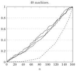
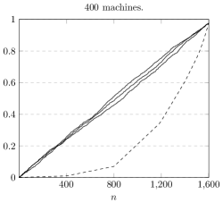
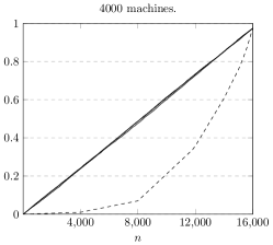
Figure 2: A graphic depicting the average load over time on the classical lower bound sequence from [1] for $40$, $400$ and $4000$ machines. The dashed line corresponds to the original adversarial order. The three solid lines corresponding to random permutations clearly approximate a straight line. Thus, sampling allows to predict the (final) average load.

Lemma 10.

[Load Lemma [5]] Let $R_{\mathrm{low}}=R_{\mathrm{low}}(m)>0$, $1\geq\varphi=\varphi(m)>0$ and $\varepsilon=\varepsilon(m)>0$ be three functions such that $\varepsilon^{-4}\varphi^{-1}R_{\mathrm{low}}^{-1}=o(m)$. Then there exists a variable $m(R_{\mathrm{low}},\varphi,\varepsilon)$ such that we have for all $m\geq m(R_{\mathrm{low}},\varphi,\varepsilon)$ and all job sets $\mathcal{J}$ with $R(\mathcal{J})\geq R_{\mathrm{low}}$ and $|\mathcal{J}|\geq m$:

$$\mathbf{P}_{\sigma\sim S_{n}}\left[\left|\frac{L_{\varphi}[\mathcal{J}^{\sigma}]}{L[\mathcal{J}]}-1\right|\geq\varepsilon\right]<\varepsilon.$$

We sketch the proof, leaving the details to Appendix A since it is technical and a slight generalization of the one found in [5]. We use geometric rounding so that we only have to deal with countably many possible job sizes. Now, jobs of any given size $p$ form a job class $\mathcal{C}=\mathcal{C}_{p}$. Using Proposition 9, we can relate their actual cardinality $n_{\mathcal{C}}$ with the $\varphi$-estimate $n_{\mathcal{C},\varphi}$. Putting everything together yields the Load Lemma, which compares the load $L$ and the load estimate $L_{\varphi}$. The lemma relies intrinsically on the lower bound $R_{\mathrm{low}}$ for $R(\mathcal{J})$. Consider a job set $\mathcal{J}$ like the one in Figure 1, only one job carries all the load while there are lots of other jobs with size zero (or negligible size $\epsilon>0$). Then $R(\mathcal{J})=\frac{1}{m}$ and a statement as in Lemma 10 could not be true for $\varepsilon<\min(1,\varphi^{-1}-1)$ since $L_{\varphi}\in\{0,\varphi^{-1}L\}$.

Figure 2 shows the behavior of the average load on three randomly chosen permutations of a classical input sequence. As predicted, this average load approaches a straight line for large number of machines. The Load Lemma is an important theoretical tool but only provides asymptotic guarantees. In Section 4.2 we explore practical guarantees for small numbers of machines.

4.2 A simple $\boldsymbol{1.75}$-competitive algorithm

We modify the semi-online algorithm $\mathrm{LightLoad}$ from the literature to obtain a very simple nearly $1.75$-competitive algorithm. For any $0\leq t\leq n$ let $M_{\mathrm{mid}}^{t}$ be a machine having the $\lfloor m/2\rfloor$-lowest load at time $t$, i.e. right before job $J_{t+1}$ is scheduled. Let $l_{\mathrm{mid}}^{t}$ be its load and let $l_{\mathrm{low}}^{t}$ be the smallest load of any machine. We recall the algorithm ${\mathrm{LightLoad[}L_{\mathrm{guess}}\mathrm{]}}$ from Albers and Hellwig [3], where the parameter $L_{\mathrm{guess}}$ is a guess for $L$.

Algorithm 1 The (semi-online) algorithm ${\mathrm{LightLoad[}L_{\mathrm{guess}}\mathrm{]}}$ [3].

1:Let $J_{t}$ be the job to be scheduled and let $p_{t}$ be its size.

2:if $l_{\mathrm{low}}^{t-1}\leq 0.25L_{\mathrm{guess}}$ or $l_{\mathrm{mid}}^{t-1}+p_{t}>1.75L_{\mathrm{guess}}$ then

3:     Schedule $J_{t}$ on any least loaded machine;

4:else schedule $J_{t}$ on $M_{\mathrm{mid}}^{t-1}$;

${\mathrm{LightLoad[}L\mathrm{]}}$ has been analyzed in the setting where the average load $L$ is known in advance, i.e. with fixed parameter $L_{\mathrm{guess}}=L$. Albers and Hellwig obtain the following:

Theorem 11 ([3]).

${\mathrm{LightLoad[}L\mathrm{]}}$ is adversarially $1.75$-competitive, i.e. for every job sequence $\mathcal{J}^{\sigma}$ with average load $L=L[\mathcal{J}]$ there holds ${\mathrm{LightLoad[}L\mathrm{]}}(\mathcal{J}^{\sigma})\leq 1.75{\mathrm{OPT}}(\mathcal{J})$.

The proof from [3] is complicated and not repeated in this paper. We need to deal with more general guesses $L_{\mathrm{guess}}$ that are slightly off. The following corollary is derived from Theorem 11 by enlarging the input sequence.

Corollary 12.

Let $\mathcal{J}^{\sigma}$ be any (ordered) input sequence and let $L_{\mathrm{guess}}\geq L[\mathcal{J}]$. Then the makespan of ${\mathrm{LightLoad[}L_{\mathrm{guess}}\mathrm{]}}$ is at most $1.75\cdot\max(L_{\mathrm{guess}},{\mathrm{OPT}}(\mathcal{J}))$.

The idea of the proof is rather simple. We can add jobs to the end of the sequence $\mathcal{J}^{\sigma}$ such that for the resulting sequence $\mathcal{J}^{\prime\sigma^{\prime}}$ there holds ${\mathrm{OPT}}(\mathcal{J}^{\prime})=\max(L_{\mathrm{guess}},{\mathrm{OPT}}(\mathcal{J}))$. We then apply Theorem 11 to see that ${\mathrm{LightLoad[}L_{\mathrm{guess}}\mathrm{]}}$ has cost at most $1.75\cdot\max(L_{\mathrm{guess}},{\mathrm{OPT}}(\mathcal{J}))$ on this sequence. Passing over to the prefix $\mathcal{J}^{\sigma}$ of $\mathcal{J}^{\prime\sigma^{\prime}}$ cannot increase this cost. A technical proof is left to Appendix B for completeness.

We also need to deal with guesses $L_{\mathrm{guess}}$ that are totally of. Since ${\mathrm{LightLoad[}L_{\mathrm{guess}}\mathrm{]}}$ only considers the least or the $\lfloor m/2\rfloor$-th least loaded machine we get by Proposition 5:

Corollary 13.

For any (ordered) sequence $\mathcal{J}^{\sigma}$ and any value $L_{\mathrm{guess}}$ the makespan of ${\mathrm{LightLoad[}L_{\mathrm{guess}}\mathrm{]}}$ is at most $(1+2R(\mathcal{J})){\mathrm{OPT}}(\mathcal{J})$. In particular, it is at most $3{\mathrm{OPT}}(\mathcal{J})$.

Adapting LightLoad to the random-order model

Let $\delta=\delta(m)=1/\log(m)$ be the margin of error our algorithm allows. We will see that our algorithm is $(1.75+O(\delta))$-competitive. In fact, any function with $\delta(m)\in\omega(m^{-1/4})$ and $\delta(m)\in o_{m}(1)$ would do. Given an input sequence $\mathcal{J}^{\sigma}$ let $\hat{L}_{\mathrm{pre}}=\hat{L}_{\mathrm{pre}}[\mathcal{J}^{\sigma}]=\frac{L_{1/4}[\mathcal{J}^{\sigma}]}{1-\delta}$ be our guess for $L$. We use the index ’pre’ since our main algorithm later will use a slightly different guess $\hat{L}$. In this section we consider the algorithm $\mathrm{LightLoadROM}={\mathrm{LightLoad[}\hat{L}_{\mathrm{pre}}\mathrm{]}}$. Let us observe first that this is indeed an online algorithm, not only a semi-online algorithm as one might expect since the if-clause uses the guess $\hat{L}_{\mathrm{pre}}$ before it is known.

Lemma 14.

The algorithm $\mathrm{LightLoadROM}$ can be implemented as an online algorithm.

Proof.

It suffices to note that the if-clause always evaluates to true for $t<n/4$, i.e. before $L_{\mathrm{guess}}=\hat{L}_{\mathrm{pre}}$ is known. Indeed, in this case $l_{\mathrm{low}}\leq 0.25L_{1/4}<0.25\hat{L}_{\mathrm{pre}}$ by Lemma 4. ∎

We now prove the main theorem. Corollary 16 follows immediately from Lemma 2.

Theorem 15.

The algorithm $\mathrm{LightLoadROM}$ is nearly $1.75$-competitive.

Corollary 16.

$\mathrm{LightLoadROM}$ is $1.75$-competitive in the secretary model for $m\rightarrow\infty$.

Figure 3: The lay of the land of the analysis. The algorithm is $(c+O(\delta))$-competitive on simple and proper stable sequences. Only the small unstable remainder (hashed) is problematic. Dashed lines mark orbits under the action of the permutation group $S_{n}$. Simple sequences stay simple under permutation. Non-simple orbits have at most an $\delta$-fraction, which is unstable (hashed). Thus, the algorithm is $(c+O(\delta))$-competitive with probability at least $1-\delta$ after random permutation.

Proof of Theorem 15.

Our analysis forms a triad, which outlines how we are going to analyze our more sophisticated $1.535$-competitive algorithm later on as well.

Analysis basics: By Corollary 13 the algorithm $\mathrm{LightLoadROM}$ is adversarially $3$-competitive. We call the input set $\mathcal{J}$ simple if $|\mathcal{J}|\leq m$ or $R[\mathcal{J}]<\frac{3}{8}$. If $|\mathcal{J}|\leq m$ every job is scheduled onto an empty machine, which is optimal. If $R[\mathcal{J}]<\frac{3}{8}$, Corollary 13 bounds the competitive ratio by $1+2R[\mathcal{J}]<1.75$. We thus are left to consider non-simple, so called proper, job sets.

Stable job sequences: We call a sequence $\mathcal{J}^{\sigma}$ stable if $L\leq\hat{L}_{\mathrm{pre}}\leq\frac{1+\delta}{1-\delta}L$ holds true. By the Load Lemma, Lemma 10, the probability of the sequence $\mathcal{J}^{\sigma}$ being stable is at least $1-\delta$ if we choose $m$ large enough and $\mathcal{J}$ proper. Here we use that $\delta(m)=1/\log(m)\in\omega(m^{-1/4})$.

Adversarial Analysis: By Corollary 12, the makespan of $\mathrm{LightLoadROM}$ on stable sequences is at most $1.75\max(\hat{L}_{\mathrm{pre}}(\mathcal{J}),{\mathrm{OPT}}(\mathcal{J}))\leq 1.75\frac{1+\delta}{1-\delta}{\mathrm{OPT}}(\mathcal{J})=\big{(}1.75+\frac{3.5\cdot\delta}{1-\delta}\big{)}{\mathrm{OPT}}(\mathcal{J}).$

Conclusion: Let $\varepsilon>0$. Since $\delta(m)\rightarrow 0$, we can choose $m$ large enough such that $\frac{3.5\delta(m)}{1-\delta(m)}\leq\varepsilon$. In particular $\mathbf{P}_{\sigma\sim S_{n}}[\mathrm{LightLoadROM}({\cal J}^{\sigma})\geq(c+\varepsilon)OPT({\cal J})]\leq\delta(m)\leq\varepsilon$ since the only sequences where the inequality does not hold are proper but not stable. This concludes the second condition of nearly competitivity. ∎

Why underestimating $L$ is actually not as bad as one may think.

So far we were careful to choose our guess $\hat{L}_{\mathrm{pre}}$ in such a way that it is unlikely to underestimate $L$ since this allowed us to prove results in a self-contained fashion, using Theorem 11 from [3] only as a black box. One should note that their analysis also allows us to tackle guesses $L_{\mathrm{guess}}<L$.

Lemma 17.

Let $\mathcal{J}^{\sigma}$ be any (ordered) input sequence and let $L_{\mathrm{guess}}=(1-\delta)L[\mathcal{J}]$ for some $\delta\geq 0$. Then the makespan of ${\mathrm{LightLoad[}L_{\mathrm{guess}}\mathrm{]}}$ is at most $1.75(1+\delta){\mathrm{OPT}}(\mathcal{J})$.

Showing this lemma requires carefully rereading the analysis of Albers and Helwig [3]. We next describe how their analysis has to be adapted to derive Lemma 17.

How to adapt the proof from [3].

Consider any input sequence $J_{1},\ldots J_{n}$. Using induction we may assume the result of the lemma to hold on the prefix $J_{1},\ldots,J_{n-1}$. In [3] they argue that the algorithm remains $1.75$-competitive if the least loaded machine had load at most $0.75L$ upon arrival of $J_{n}$. By a similar reasoning the less strict statement of Lemma 17 holds if the least loaded machine had load at most $0.75L+1.75\delta L$ at that time. Thus we are left to consider the case that its load is $0.75L+1.75\delta L+\epsilon L$ for some $0<\epsilon<0.25-1.75\delta$. Following the arguments [3], it suffices to show that every machine received a job of size $0.5L+\epsilon L$. The statement of Lemma 1 in [3] needs to be weakened to ’At time $t_{j_{0}}$ the least loaded machine had load at most $(0.25+1.75\delta)L$.’ The proof of the lemma remains mostly the same. The only change occurs in the induction step. Here, the size of a job causing a machine to reach load $0.75L+\delta L+\epsilon L$ and, in addition, the corresponding decrease in potential is only $(1-1.75\delta)L$. Similarly, the statement of Lemma 2 needs to be refined to ’the $j_{0}$-th least loaded machine had load at most $(1.25+1.75\delta)L-\epsilon L=1.75L_{\mathrm{guess}}-0.5L-\epsilon L$.’ The proof of Lemma 2 stays the same. Using these modifications, the rest of the analysis of [3] can be applied to conclude the proof. ∎

Theorem 18.

Let $\mathcal{J}^{\sigma}$ be any (ordered) input sequence. The makespan of $\mathrm{LightLoadROM}$ on $\mathcal{J}^{\sigma}$ is $1.75\cdot\left(1+\frac{|\hat{L}_{\mathrm{pre}}[\mathcal{J}^{\sigma}]-L|}{L}\right){\mathrm{OPT}}$.

Proof.

On input permutation $\mathcal{J}^{\sigma}$ the competitive ratio of our algorithm is at most $1.75+\frac{\left|L_{1/4}-L\right|}{L}$ by Corollary 12 if $L_{1/4}\geq L$. Else, recall that ${\mathrm{OPT}}\geq L$ and apply Lemma 17. ∎

Let us assume for simplicity that the input length $n$ is divisible by $4$. We can always add up to three jobs of size $0$ to obtain such a result. This ’adding’ can be simulated by an online algorithm. Recall that the absolute mean deviation of a random variable $X$ that has nonzero expectation is defined as $\mathrm{MD}[X]=\mathbf{E}\left[\left|X-\mathbf{E}[X]\right|\right]$ and its normalized absolute mean deviation is $\mathrm{NMD}[X]=\frac{\mathbf{E}\left[\left|X-\mathbf{E}[X]\right|\right]}{\mathbf{E}[X]}$. In particular, $\mathrm{NMD}[L_{1/4}]=\frac{\mathbf{E}_{\sigma\sim S_{N}}\left[\left|L_{1/4}-L\right|\right]}{L}.$ From the previous theorem we obtain:

Theorem 19.

On input set $\mathcal{J}$ the competitive ratio of $\mathrm{LightLoadROM}$ in the random-order model is at most $1.75(1+\mathrm{NMD}(\hat{L}_{\mathrm{pre}}))$. If $n\leq m$ or $R(\mathcal{J})\leq\frac{3}{8}$, then ${\mathrm{LightLoad[}L_{1/4}\mathrm{]}}$ is already $1.75$-competitive.

Proof.

The first statement follows from Theorem 18 by taking expected values. If $n\leq m$, the algorithm ${\mathrm{LightLoad[}L_{1/4}\mathrm{]}}$ places every job on a separate machine and is thus optimal. If $R(\mathcal{J})\leq\frac{3}{8}$, it is $1.75$-competitive by Corollary 13. ∎

We will now provide estimates on $\mathrm{NMD}(\hat{L}_{\mathrm{pre}})$. Figure 4 depicts practical estimates, while our analysis will focus on theoretical bounds.

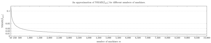
Figure 4: The extra cost for small numbers of machines. The graph shows an estimation of $\mathrm{NMD}(\hat{L}_{\mathrm{pre}})$ on the lower bound sequence from [1] based on $10,000$ random samples. The curve indicates good performance of $\mathrm{LightLoadROM}$ in practice by Theorem 19.

Given any job set $\mathcal{J}$ of size $n>m$ and $R(\mathcal{J})\geq\frac{3}{8}$ we are left to estimate this normalized standard deviation of $L_{1/4}$. One observes that $\mathrm{NMD}[L_{1/4}]$ does not change if we scale all jobs by a common factor $\lambda>0$. By choosing $\lambda=L^{-1}$ we may wlog. assume that $L=1$. In particular, $\mathrm{NMD}[L_{1/4}]=\mathrm{MD}[L_{1/4}]$. Now $R(\mathcal{J})\geq\frac{3}{8}$ implies that all jobs have size at most $8/3$. The following lemma allows us to reduce ourselves to particularly easy job instances.

Lemma 20.

Consider two jobs $J_{a},J_{b}\in\mathcal{J}$ of sizes $p_{a}\leq p_{b}$ and $0\leq\varepsilon\leq p_{a}$. If we set the size of $J_{a}$ to $p_{a}-\varepsilon$ and the size of $J_{b}$ to $p_{b}+\varepsilon$, then $\mathrm{MD}(L_{1/4})$ does not decrease.

Proof.

Consider $\mathrm{MD}(L_{1/4})(p_{1},\ldots,p_{n})=\mathbf{E}[|L_{1/4}-L|](p_{1},\ldots,p_{n})$ as a function on the job sizes $p_{1},\ldots,p_{n}$. This function is convex since it is a convex combination of the convex functions $|L_{1/4}[\sigma]-L|$ for all $\sigma\in S_{n}$. ∎

We apply the previous lemma to any pairs of $J_{a},J_{b}\in\mathcal{J}$ of sizes $0<p_{a}\leq p_{b}<8/3$ to set either $p_{a}=0$ or $p_{b}=8/3$. We then repeat this process till all jobs but one last one have either size $0$ or $8/3$. So far at most $\left\lfloor\frac{3m}{8}\right\rfloor$ jobs have size $8/3$ since by assumption $L=1$. Using again the fact that $\mathrm{MD}[L_{1/4}]$ is convex in the size of jobs, setting the size $p$ of this remaining job to at least one of the values $0$ or $8/3$ cannot decrease $\mathrm{MD}[L_{1/4}]$. Let us do so. This breaks the assumption that $L=1$, which is why we consider $\mathrm{MD}$ instead of $\mathrm{NMD}$. Let $K=K(n)$ be the number of jobs of size $8/3$. Then $K$ is either $\left\lfloor\frac{3m}{8}\right\rfloor$ or $\left\lfloor\frac{3m}{8}\right\rfloor+1$. Let $X\sim\mathrm{HyperGeom}(n,K,n/4)$, in other words $X$ corresponds to drawing $n/4$ elements without replacement from a population of size $n$ that contains precisely $K$ successes. Then $L_{1/4}=\frac{8X}{3m}$ for our modified job set. Since all modifications never caused $\mathrm{MD}[X]$ to decrease we have shown so far:

Lemma 21.

Let $\mathcal{J}$ be a job set of size $n>m$ with $R(\mathcal{J})\leq\frac{3}{8}$. Then we can choose $K$ either $\left\lfloor\frac{3m}{8}\right\rfloor$ or $\left\lfloor\frac{3m}{8}\right\rfloor+1$ such that for $X\sim\mathrm{HyperGeom}(n,K,n/4)$ there holds $\mathrm{NMD}[L_{1/4}]\leq\frac{8}{3m}\mathrm{MD}[X]$.

It is possible to evaluate the standard mean deviation of $X\sim\mathrm{HyperGeom}(n,K,n/4)$ directly using the techniques in [17]. Since such an analysis is quite complex we present a simpler proof, which yields somewhat worse bounds.

Lemma 22.

Let $X\sim\mathrm{HyperGeom}(n,K,n/4)$ and $Y\sim\mathrm{Bin}(K,1/4)$ then $\mathrm{MD}(X)\leq\mathrm{MD}(Y)$.

Proof.

Indeed, both random variables correspond to $K$ draws from a population of size $n$ that contains $n/4$ successes. For $X$ these draws occur without replacement, while for $Y$ these are draws with replacement. Let $X_{i}$ respectively $Y_{i}$ be the respective random variable, which only considers the first $i$ draws for $0\leq i\leq K$. We can show via induction that the random variable $|Y_{i}-i/4|$ dominates $|X_{i}-i/4|$ by a case distinction on the possible values of $Y_{i-1}-(i-1)/4$ and $X_{i-1}-(i-1)/4$. Thus, the random variable $|Y-\mathbf{E}[Y]|$ dominates $|X-\mathbf{E}[X]|$. This implies $\mathrm{MD}(Y)=\mathbf{E}[|Y-\mathbf{E}[Y]|]\geq\mathbf{E}[|X-\mathbf{E}[X]|]=\mathrm{MD}(X)$. ∎

Given $Y\sim\mathrm{Bin}(K,p)$, we are interested in $p=1/4$, let $\mathrm{bin}(k,K,p)=P[Y=k]={K\choose k}p^{k}(1-p)^{K-k}$. Then we can evaluate the median deviation of $Y$ using de Moivre’s theorem.

Theorem 23 (de Moivre).

$\mathrm{MD}(Y)=2\lfloor pK+1\rfloor(1-p)\mathrm{bin}(\lfloor pK+1\rfloor,K,p)$ for $Y\sim\mathrm{Bin}(K,p)$.

A proof of the theorem can be found in [17]. Consider $Y\sim\mathrm{Bin}(K,1/4)$ and set $k=\lfloor K/4+1\rfloor$. Using Stirling’s Approximation we derive

$$\mathrm{MD}(Y) =\lfloor 2k\rfloor\cdot 3/4\cdot\mathrm{bin}\left(k,K,1/4\right)$$

$$=(1+o_{K}(1))\frac{3}{8}K\frac{K!}{k!(K-k)!}(1/4)^{k}(3/4)^{K-k}$$

$$=(1+o_{K}(1))\frac{3}{8}K\frac{\sqrt{2\pi K}\left(\frac{K}{e}\right)^{K}}{\sqrt{2\pi k}\left(\frac{k}{e}\right)^{k}\sqrt{2\pi(K-k)}\left(\frac{K-k}{e}\right)^{K-k}}\left(\frac{1}{4}\right)^{k}\left(\frac{3}{4}\right)^{K-k}$$

$$=(1+o_{K}(1))\frac{3}{8}K\sqrt{\frac{K}{2\pi k(K-k)}}\left(\frac{K}{4k}\right)^{k}\left(\frac{3}{4}\frac{K}{K-k}\right)^{K-k}.$$

Recall $K/4<k\leq K/4+1$. Thus $\left(\frac{K}{4k}\right)^{k}\leq 1$ and $\left(\frac{3}{4}\frac{K}{K-k}\right)^{K-k}\leq\left(1+\frac{1}{3K/4-1}\right)^{3K/4}=e+o_{K}(1)$. We get that $\mathrm{MD}(Y)\leq(1+o_{K}(1))\frac{3e}{8}K\sqrt{\frac{K}{2\pi k(K-k)}}$. Recall that $K=\left\lfloor\frac{3m}{8}\right\rfloor$ or $K=\left\lfloor\frac{3m}{8}\right\rfloor+1$. In particular, $K=(1+o_{m}(1))\frac{8}{3}m$ and $k=(1+o_{m}(1))\frac{2}{3}m$ . Thus

$$\mathrm{MD}(Y)=(1+o_{m}(1))\frac{3e}{8}\frac{8m}{3}\sqrt{\frac{8m/3}{2\pi 2m/3\cdot(1m/3)}}=(1+o_{m}(1))\sqrt{\frac{6e^{2}m}{\pi}}.$$

Consider any job set $\mathcal{J}$ of size $n$ with $R(\mathcal{J})\leq\frac{3}{8}$. Combining the previous bound with Lemma 21 and Lemma 22 yields

$$\mathrm{NMD}[L_{1/4}]\leq\frac{8}{3m}\mathrm{MD}[X]=(1+o_{m}(1))\frac{8}{3m}\sqrt{\frac{6e^{2}m}{\pi}}<\frac{10.02+o_{m}(1)}{\sqrt{m}}.$$

This bound allows to establish a competitive ratio in the random-order model.

Theorem 24.

The competitive ratio of $\mathrm{LightLoadROM}$ in the random-order model is $1.75+\frac{18}{\sqrt{m}}+O\left(\frac{1}{m}\right)$.

Proof.

This is a consequence of Theorem 19 and the prior bound on $\mathrm{NMD}[L_{1/4}]$. ∎

Remark 1.

The constant in the previous theorem is far from optimal. As mentioned before a first improvement can be derived by estimating the absolute mean average deviation of the hypergeoemtric distribution directly using the techniques from [17]. A much stronger improvement results from filtering out huge jobs reducing essentially to the case that $R(\mathcal{J})=1$. Given any guess $L_{\mathrm{guess}}$ let $\delta(L_{\mathrm{guess}})$ be $L-L_{\mathrm{guess}}$ if $L_{\mathrm{guess}}\leq L$; $L_{\mathrm{guess}}-{\mathrm{OPT}}$ if $L_{\mathrm{guess}}>{\mathrm{OPT}}$; and $0$ else. Combining Corollary 12 and Lemma 17 yields that ${\mathrm{LightLoad[}L_{\mathrm{guess}}\mathrm{]}}$ is $1.75(1+\delta(L_{\mathrm{guess}}))$-competitive. So far, we picked for $L_{\mathrm{guess}}$ an estimator for $L$. But besides $L$ we could also try to estimate the lower bound for ${\mathrm{OPT}}$, that is we could consider $B_{\mathrm{pre}}[\mathcal{J}^{\sigma}]=\max\left(L_{1/4}[\mathcal{J}^{\sigma}],p^{n/4}_{\mathrm{max}}[\mathcal{J}^{\sigma}]\right)$, which is similar to how we estimate ${\mathrm{OPT}}$ in our main algorithm. The nature of the guess $B_{\mathrm{pre}}[\mathcal{J}^{\sigma}]$ ensures that only few job have size exceeding $B_{\mathrm{pre}}$; only $4$ in expectation. A more careful analysis reveals that the competitive ratio of ${\mathrm{LightLoad[}B_{\mathrm{pre}}\mathrm{]}}$ is in fact $1.75+\frac{4.4}{\sqrt{m}}+\frac{7}{m}+O\left(m^{-3/2}\right)$ in the random-order model.

5 The new, nearly 1.535-competitive algorithm

Figure 5: The 1.535-competitive algorithm. First, few jobs are sampled. Then, the algorithm decides between two strategies. The Critical-Job-Strategy tries to schedule critical jobs ahead of time. The Least-Loaded-Strategy follows a greedy approach, which reserves some machines for large jobs. Sometimes, we realize very late that the Critical-Job-Strategy does not work and have to switch to the Least-Loaded-Strategy ’on the fly’. We never switch in the other direction.

Our new algorithm achieves a competitive ratio of $c=\frac{1+\sqrt{13}}{3}\approx 1.535$. Let $\delta=\delta(m)=\frac{1}{\log(m)}$ be the margin of error our algorithm allows. Throughout the analysis it is mostly sensible to treat $\delta$ as a constant and forget about its dependency on $m$. Our algorithm maintains a certain set $\mathcal{M}_{\mathrm{res}}$ of $\lceil\delta m\rceil$ reserve machines. Their complement, the principal machines, are denoted by $\mathcal{M}$. Let us fix an input sequence $\mathcal{J}^{\sigma}$. Let $\hat{L}=\hat{L}[\mathcal{J}^{\sigma}]=L_{\delta^{2}}[\mathcal{J}^{\sigma}]$. For simplicity, we hide the dependency on $\mathcal{J}^{\sigma}$ whenever possible. Our online algorithm uses $B=\max\left(p^{\delta^{2}n}_{\mathrm{max}},\hat{L}\right)$ as an estimated lower bound for ${\mathrm{OPT}}$, which is known after the first $\lfloor\delta^{2}n\rfloor$ jobs are treated. Our algorithm uses geometric rounding implicitly. Given a job $J_{t}$ of size $p_{t}$ let $f(p_{t})=(1+\delta)^{\left\lfloor\log_{1+\delta}p_{t}\right\rfloor}$ be its rounded size. We also call $J_{t}$ an $f(p_{t})$-job. Using rounded sizes, we introduce job classes. Let $p_{\mathrm{small}}=c-1=\frac{\sqrt{13}-2}{3}\approx 0.535$ and $p_{\mathrm{big}}=\frac{c}{2}=\frac{1+\sqrt{13}}{6}\approx 0.768$. Then we call job $J_{t}$

• small if $f(p_{t})\leq p_{\mathrm{small}}B$ and critical else,

• big if $f(p_{t})>p_{\mathrm{big}}B$,

• medium if $J$ is neither small nor big, i.e. $p_{\mathrm{small}}B\leq f(p_{t})\leq p_{\mathrm{big}}B$,

• huge if its (not-rounded) size exceeds $B$, i.e. $B<p_{t}$, and normal else.

Consider the sets $\mathcal{P}_{\mathrm{med}}=\{(1+\delta)^{i}\mid(1+\delta)^{-1}p_{\mathrm{small}}B<(1+\delta)^{i}\leq p_{\mathrm{big}}B\}$ and $\mathcal{P}_{\mathrm{big}}=\{(1+\delta)^{i}\mid p_{\mathrm{big}}B<(1+\delta)^{i}\leq B\}$ corresponding to all possible rounded sizes of medium respectively big jobs, excluding huge jobs. Let $\mathcal{P}=\mathcal{P}_{\mathrm{med}}\cup\mathcal{P}_{\mathrm{big}}$. This subdivision gives rise to a weight function, which will be important later. Let $w(p)=1/2$ for $p\in\mathcal{P}_{\mathrm{med}}$ and $w(p)=1$ for $p\in\mathcal{P}_{\mathrm{big}}$. The elements $p\in\mathcal{P}$ define job classes $\mathcal{C}_{p}\subseteq\mathcal{J}$ consisting of all $p$-jobs, i.e. jobs of rounded size $p$. By some abuse of notation, we call the elements in $\mathcal{P}$ ’job classes’, too. Using the notation from Section 4.1 we set $n_{p}=n_{\mathcal{C}_{p}}=|\mathcal{C}_{p}|$ and $\hat{n}_{p}=n_{\mathcal{C}_{p},\delta^{2}}=|\{J_{\sigma(j)}\mid\sigma(j)\leq\delta^{2}n\land J_{\sigma(j)}\textrm{ is a $p$-job}\}|$. We want to use the values $\hat{n}_{p}$, which are available to an online algorithm quite early, to estimate the values $n_{p}$, which accurately describe the set of critical jobs. First, $\delta^{-2}\hat{n}_{p}$ comes to mind as an estimate for $n_{p}$. Yet, we need a more complicated guess: $c_{p}=\max\left(\left\lfloor\left(\delta^{-2}\hat{n}_{p}-m^{3/4}\right)w(p)\right\rfloor,\hat{n}_{p}\right)w(p)^{-1}$. It has three desirable advantages. First, for every $p\in\mathcal{P}$ the value $c_{p}$ is close to $n_{p}$ with high probability, but, opposed to $\delta^{-2}\hat{n}_{p}$, unlikely to exceed it. Overestimating $n_{p}$ turns out to be far worse than underestimating it. Second, $w(p)c_{p}$ is an integer and, third, we have $c_{p}\geq\hat{n}_{p}w(p)^{-1}$. A fundamental fact regarding the values $(c_{p})_{p\in\mathcal{P}}$ and $B$ is, of course, that they are known to the online algorithm once $\lfloor\delta^{2}n\rfloor$ jobs are scheduled.

Statement of the algorithm:

If there are less jobs than machines, i.e. $n\leq m$, it is optimal to put each job onto a separate machine. Else, a short sampling phase greedily schedules each of the first $\lfloor\delta^{2}n\rfloor$ jobs to the least loaded principal machine $M\in\mathcal{M}$. Now, the values $B$ and $(c_{p})_{p\in\mathcal{P}}$ are known. Our algorithm has to choose between two strategies, the Least-Loaded-Strategy and the Critical-Job-Strategy, which we will both introduce subsequently. It maintains a variable strat, initialized to Critical, to remember its choice. If it chooses the Critical-Job-Strategy, some additional preparation is required. It may at any time discover that the Critical-Job-Strategy is not feasible and switch to the Least-Loaded-Strategy but it never switches the other way around.

Algorithm 2 The complete algorithm: How to schedule job $J_{t}$.

1:strat is initialized to Critical, $J_{t}$ is the job to be scheduled.

2:if $n\leq m$ then Schedule $J_{t}$ on any empty machine;

3:else if $t\leq\varphi n$ then schedule $J_{t}$ on a least loaded machine in $\mathcal{M}$;$\triangleright$ Sampling phase

4:else

5:     if we have $t=\lfloor\varphi n\rfloor+1$ then

6:         if $\sum_{p\in\mathcal{P}}w(p)c_{p}>m$ then $\textsc{strat}\leftarrow\textsc{Least-Loaded}$

7:         else proceed with the Preparation for the Critical-Job-Strategy (Algorithm 4);               

8:     if $\textsc{strat}=\textsc{Critical}$ then proceed with the Critical-Job-Strategy (Algorithm 5);

9:     else proceed with the Least-Loaded-Strategy (Algorithm 3);      

Figure 6: The Least-Loaded-Strategy schedules jobs greedily. A few machines are reserved for unexpected huge jobs, such as the largest job, which is unlikely to arrive in the sampling phase.

The Least-Loaded-Strategy places any normal job on a least loaded principal machine. Huge jobs are scheduled on any least loaded reserve machine. This machine will be empty, unless we consider rare worst-case orders.

Algorithm 3 The Least-Loaded-Strategy: How to schedule job $J_{t}$.

1:if $J_{t}$ is huge then schedule $J_{t}$ on any least loaded reserve machine;

2:else schedule $J_{t}$ on any least loaded principal machine;

For the Critical-Job-Strategy we introduce $p$-placeholder-jobs for every size $p\in\mathcal{P}$. Sensibly, the size of a $p$-placeholder-job is $p$. During the Critical-Job-Strategy we treat placeholder-jobs similar to real jobs. The anticipated load $\tilde{l}_{M}^{t}$ of a machine $M$ at time $t$ is the sum of all jobs on it, including placeholder-job, opposed to the common load $l_{M}^{t}$, which does not take the latter into account. Note that $\tilde{l}_{M}^{t}$ defines a pseudo-load as introduced in Section 4.

Figure 7: The Critical-Job-Strategy. Each machine gets either two medium, one large or no critical job. Placeholder jobs (dotted) are assigned during the Preparation and reserve space for critical jobs yet to come. Processing volume of small jobs (dark) ’on the bottom’ arrived during the sampling phase. Reserve machines accommodate huge jobs or, possibly, jobs without matching placeholders.

During the Preparation for the Critical-Job-Strategy the algorithm maintains a counter $c_{p}^{\prime}$ of all $p$-jobs scheduled so far (including placeholders). A job class $p\in\mathcal{P}$ is called unsaturated if $c_{p}^{\prime}\leq c_{p}$. First, we add unsaturated medium placeholder-jobs to any principal machine that already contains a medium real job from the sampling phase. We will see in Lemma 25 that such an unsaturated medium job class always exists. Now, let $m_{\mathrm{empty}}$ be the number of principal machines which do not contain critical jobs. We prepare a set $\mathcal{J}_{\mathrm{rep}}$ of cardinality at most $m_{\mathrm{empty}}$, which we will then schedule onto these machines. The set $\mathcal{J}_{\mathrm{rep}}$ may contain single big placeholder-jobs or pairs of medium placeholder-jobs. We greedily pick any unsaturated job class $p\in\mathcal{P}$ and add a $p$-placeholder-job to $\mathcal{J}_{\mathrm{rep}}$. If $p$ is medium, we pair it with a job belonging to any other, not necessarily different, unsaturated medium job class. Such a job class always exists by Lemma 25. We stop once all job classes are saturated or if $|\mathcal{J}_{\mathrm{rep}}|=m_{\mathrm{empty}}$. We then assign the elements in $\mathcal{J}_{\mathrm{rep}}$ to machines. We iteratively pick the element $e\in\mathcal{J}_{\mathrm{rep}}$ of maximum size and assign the corresponding jobs to the least loaded principal machine, which does not contain critical jobs yet. Sensibly, the size of a pair of jobs in $\mathcal{J}_{\mathrm{rep}}$ is the sum of their individual sizes. We repeat this until all jobs and job pairs in $\mathcal{J}_{\mathrm{rep}}$ are assigned to some principal machine.

Algorithm 4 Preparation for the Critical-Job-Strategy.

1:while there is a machine $M$ containing a single medium job do

2:     Add a placeholder $p$-job for an unsaturated size class $p\in\mathcal{P}_{\mathrm{med}}$ to $M$; $c_{p}^{\prime}\leftarrow c_{p}^{\prime}+1$;

3:while there is an unsaturated size class $p\in\mathcal{P}$ and $|\mathcal{J}_{\mathrm{rep}}|<m_{\mathrm{empty}}$ do

4:     Pick an unsaturated size class $e=p\in\mathcal{P}$ with $c_{p}^{\prime}$ minimal; $w(e)\leftarrow p$; $c_{p}^{\prime}\leftarrow c_{p}^{\prime}+1$;

5:     if $p$ is medium then pick $q\in\mathcal{P}_{\mathrm{med}}$ unsaturated. $e\leftarrow(p,q)$; $w(e)\leftarrow p+q$; $c_{q}^{\prime}\leftarrow c_{q}^{\prime}+1$;      

6:     Add $e$ to $\mathcal{J}_{\mathrm{rep}}$;

7:while $\mathcal{J}_{\mathrm{rep}}\neq\emptyset$ do

8:     Pick a least loaded machine $M\in\mathcal{M}$, which does not contain a critical job yet;

9:     Pick $e\in\mathcal{J}_{\mathrm{rep}}$ of maximum size $w(e)$ and add the jobs in $e$ to $M$;

10:     $\mathcal{J}_{\mathrm{rep}}\leftarrow\mathcal{J}_{\mathrm{rep}}\setminus\{e\}$;

Lemma 25.

In line 2 and 5 of Algorithm 4 there is always an unsaturated medium size class available. Thus, Algorithm 4, the Preparation for the Critical-Job-Strategy, is well defined.

Proof.

Concerning line 2, there are precisely $\sum_{p\in\mathcal{P}_{\mathrm{med}}}\hat{n}_{p}$ machines with critical jobs while there are at least $\sum_{p\in\mathcal{P}_{\mathrm{med}}}(c_{p}-\hat{n}_{p})\geq\sum_{p\in\mathcal{P}_{\mathrm{med}}}\hat{n}_{p}$ placeholder-jobs available to fill them. Here we make use of the fact that for medium jobs $p\in\mathcal{P}_{\mathrm{med}}$ we have $c_{p}\geq\hat{n}_{p}w(p)^{-1}=2\hat{n}_{p}$.

Concerning line 5, observe that so far every machine and every element in $\mathcal{J}_{\mathrm{rep}}$ contains an even number of medium jobs. If the placeholder picked in line 4 was the last medium job remaining, $\sum_{p\in\mathcal{P}_{\mathrm{med}}}c_{p}$ would be odd. But this is not the case since every $c_{p}$ for $p\in\mathcal{P}_{\mathrm{med}}$ is even. ∎

After the Preparation is done, the Critical-Job-Strategy becomes straightforward. Each small job is scheduled on a principal machines with least anticipated load, i.e. taking placeholders into account. Critical jobs of rounded size $p\in\mathcal{P}$ replace $p$-placeholder-jobs whenever possible. If no such placeholder exists anymore, critical jobs are placed onto the reserve machines. Again, we try pair up medium jobs whenever possible. If no suitable machine can be found among the reserve machines, we have to switch to the Least-Loaded-Strategy. We say that the algorithm fails if it ever reaches this point. In this case, it should rather have chosen the Least-Loaded-Strategy to begin with. Since all reserve machines are filled at this point, the Least-Loaded-Strategy is impeded, too. The most difficult part of our analysis shows that, excluding worst-case orders, this is not a problem on job sets that are prone to cause failing.

Algorithm 5 The Critical-Job-Strategy.

1:if $J_{t}$ is medium or big then let $p$ denote its rounded size;

2:     if there is a machine $M$ containing a $p$-placeholder-job $J$ then

3:         Delete the $p$-placeholder-job $J$ and assign $J_{t}$ to $M$;

4:     else if $J_{t}$ is medium and there exists $M\in\mathcal{M}_{\mathrm{res}}$ containing a single medium job then

5:         Schedule $J_{t}$ on $M$;

6:     else if there exists an empty machine $M\in\mathcal{M}_{\mathrm{res}}$ then schedule $J_{t}$ on $M$;

7:     else $\textsc{stat}\leftarrow\textsc{Least-Loaded}$; $\triangleright$ We say the algorithm fails.

8:         use the Least-Loaded-Strategy (Algorithm 3) from now on;      

9:else assign $J_{t}$ to the least loaded machine in $\mathcal{M}$ (take placeholder jobs into account);

6 Analysis of the algorithm

Theorem 26 is main result of the paper. Corollary 27 follows immediately by Lemma 2.

Theorem 26.

Our algorithm is nearly $c$-competitive. Recall that $c=\frac{1+\sqrt{13}}{3}\approx 1.535$.

Corollary 27.

Our algorithm is $c$-competitive in the secretary model as $m\rightarrow\infty$.

The analysis of our algorithm proceeds along the same three reduction steps used in the proof of Theorem 15. First, we assert that our algorithm has a bounded adversarial competitive ratio, which approaches $1$ as $R(\mathcal{J})\rightarrow 0$. Not only does this lead to the first condition of nearly competitiveness, it also enables us to introduce simple job sets on which we perform well due to basic considerations resulting from Section 4.

Definition 28.

A job set $\mathcal{J}$ is called simple if $R(\mathcal{J})\leq\frac{(1-\delta)\delta^{3}}{2(\delta^{2}+1)}(2-c)$ or if it consists of at most $m$ jobs. Else, we call it proper. We call any ordered input sequence $\mathcal{J}^{\sigma}$ simple respectively proper if the underlying set $\mathcal{J}$ has this property.

Next we are going to sketch out main proof introducing three Main Lemmas. These follow the three proof steps introduced in the proof of Corollary 16.

Main Lemma 1.

In the adversarial model our algorithm has competitive ratio $4+O(\delta)$ on general input sequences and $c+O(\delta)$ on simple sequences.

The proof is discussed later. We are thus reduced to treating proper job sets. In the second reduction we introduce stable sequences. These have many desirable properties. Most notably, they are suited to sampling. We leave the formal definition to Section 6.2 since it is rather technical. The second reduction shows that stable sequences arise with high probability if one orders a proper job set uniformly randomly.

Formally, for $m$ the number of machines, let $P(m)$ be the maximum probability by which the permutation of any proper sequence may not be stable, i.e.

$$P(m)=\sup\limits_{\mathcal{J}\textrm{ proper}}\mathbf{P}_{\sigma\sim S_{n}}\left[\mathcal{J}^{\sigma}\textrm{ is not stable}\right].$$

The second main lemma asserts that this probability vanishes as $m\rightarrow\infty$.

Main Lemma 2.

$\lim\limits_{m\rightarrow\infty}P(m)=0$.

In other words, non-stable sequences are very rare and of negligible impact in random-order analyses. Thus, we only need to consider stable sequences. In the final, third, step we analyze our algorithm on these. This analysis is quite general. In particular, it does not rely further on the random-order model. Instead, we work with worst-case stable input sequences, i.e. we allow the adversary to present any (ordered) stable input sequence.

Main Lemma 3.

Our algorithm is adversarially $(c+O(\delta))$-competitive on stable sequences.

These three main lemmas allow us to conclude the proof of Theorem 26.

Proof of Theorem 26.

By 1, the first condition of nearly competitiveness holds, i.e. our algorithm has a constant competitive ratio. Moreover, by 1 and 3, given $\varepsilon>0$, we can pick $m_{0}(\varepsilon)$ such that our algorithm is $(c+\varepsilon)$-competitive on all sequences that are stable or simple if there are at least $m_{0}(\varepsilon)$ machines. Here, we need that $\delta(m)\rightarrow 0$ for $m\rightarrow\infty$. This implies that for $m\geq m_{0}(\varepsilon)$ the probability of our algorithm not being $(c+\varepsilon)$-competitive is at most $P(m)$, the maximum probability with which a random permutation of a proper, i.e. non-simple, input sequence is not stable. By 2, we can find $m(\varepsilon)\geq m_{0}(\varepsilon)$ such that this probability is less than $\varepsilon$. This satisfies the second condition of nearly competitiveness. ∎

6.1 The adversarial case. Proof of 1

Recall that the anticipated load $\tilde{l}_{M}^{t}$ of a machine $M$ at time $t$ denotes its load including placeholder-jobs. It satisfies the definition of a pseudo-load as introduced in Section 4. We obtain the following two bounds on the average anticipated load $\tilde{L}=\sup_{t}\frac{1}{m}\sum_{M}\tilde{l}_{M}^{t}$.

Lemma 29.

We have $\tilde{L}\leq L+2p_{\mathrm{max}}$. In particular $\tilde{R}(\mathcal{J})\leq 3$.

Proof.

First note that every placeholder-job has at most the size of some job encountered during the sampling phase. In particular, the size of any placeholder-job is at most $p_{\mathrm{max}}$. Since there are at most two placeholder-jobs on each machine, the total processing time of all placeholder-jobs is at most $2mp_{\mathrm{max}}$. The total processing time of real jobs is at most $mL$. Thus the total processing time of all placeholder and real jobs scheduled at any time cannot exceed $m(L+2p_{\mathrm{max}})$. In particular, at any time $t$, we have $\frac{1}{m}\sum_{M}\tilde{l}_{M}^{t}\leq\frac{1}{m}m(L+2p_{\mathrm{max}})$. Thus, $\tilde{L}\leq L+2p_{\mathrm{max}}$. For the second part we conclude that $\tilde{R}(\mathcal{J})\leq\min\left(\frac{\tilde{L}}{p_{\mathrm{max}}},\frac{\tilde{L}}{L}\right)\leq\min\left(\frac{L}{p_{\mathrm{max}}}+2,2\frac{p_{\mathrm{max}}}{L}+1\right)\leq 3.$ ∎

Lemma 30.

We have $\tilde{L}\leq\left(1+\frac{1}{\delta^{2}}\right)L$, in particular $\tilde{R}(\mathcal{J})\leq\left(1+\frac{1}{\delta^{2}}\right)R(\mathcal{J})$.

Let us first show the following stronger lemma.

Lemma 31.

The total size of the placeholder-jobs is at most $m\hat{L}$. In particular, $\tilde{L}\leq L+\hat{L}$.

Proof of Lemma 31.

For every $p\in\mathcal{P}$ we schedule at most $c_{p}\leq\delta^{-2}\hat{n}_{p}$ placeholder-jobs of type $p$. Thus, the total size of the placeholder-jobs is at most $\sum_{p\in\mathcal{P}}\delta^{-2}\hat{n}_{p}\leq m\hat{L}.$ The total size of all real jobs is precisely $mL$. Since $\tilde{L}$ is at most $\frac{1}{m}$-times the total processing time of all jobs, we have $\tilde{L}\leq\frac{1}{m}(mL+m\hat{L})$. ∎

Proof of Lemma 30.

Observe that $\hat{L}=L_{\delta^{2}}\leq\delta^{-2}L$. Then, the bound follows from Lemma 31. ∎

We call a machine critical if it receives a critical job from the Critical-Job-Strategy but no small job after the sampling phase. Else, we call it general. General machines can be analyzed using Proposition 5 and 8. Critical machines need more careful arguments.

Lemma 32.

At any time, the load of any general machine is at most $\left(\frac{\tilde{R}(\mathcal{J})}{1-\delta}+1+2\delta\right){\mathrm{OPT}}(\mathcal{J})$.

Proof.

For sequences of length $n\leq m$ our algorithm is optimal. Hence assume $n>m$.

During the sampling phase and the Least-Loaded-Strategy, our algorithm always uses either a least loaded machine or a least loaded principal machine. Both lie among the $\lfloor\delta m\rfloor+1$ least loaded machines. By Proposition 5 this cannot cause any load to exceed $\left(\frac{m}{m-\lfloor\delta m\rfloor}R(\mathcal{J})+1\right){\mathrm{OPT}}(\mathcal{J})\leq\left(1+\frac{R(\mathcal{J})}{1-\delta}\right){\mathrm{OPT}}(\mathcal{J})$. Observing that $\tilde{R}(\mathcal{J})\geq R(\mathcal{J})$, see Lemma 6, the lemma holds for every machine that does not receive its last job during the Critical-Job-Strategy.

Now consider a general machine $M$, which received its last job during the Critical-Job-Strategy. Since it is a general machine, it also received a small job during the Critical-Job-Strategy. Let $J$ be the last small job it received. Right before receiving $J$ machine $M$ must have been a principal machine of least anticipated load. In total, it had at most the $(\lfloor\delta m\rfloor+1)$-smallest anticipated load. By Proposition 8 its anticipated load was at most $\left(\frac{\tilde{R}(\mathcal{J})}{1-\delta}+1\right){\mathrm{OPT}}(\mathcal{J})$ after receiving $J$. Afterwards machine $M$ may have received up to two critical jobs, which replaced placeholder-jobs. Since these jobs had at most $(1+\delta)$-times the size of the job they replaced. The load-increase is at most $\delta p_{\mathrm{max}}\leq\delta{\mathrm{OPT}}$ for each of these two jobs. ∎

We can now consider critical machines.

Lemma 33.

The load of a reserve machine is at most $\min(\max((1+\delta)cB,p_{\mathrm{max}}),2p_{\mathrm{max}})$ till it receives a job from the Least-Loaded-Strategy. Critical reserve machines in particular fulfill this condition.

Proof.

Every critical reserve machine receives either one big job or at most two medium ones, until the Least-Loaded-Strategy is applied. The second bound, $2p_{\mathrm{max}}$, follows immediately from that. The first bound follows from the fact that a single big job has size at most $p_{\mathrm{max}}$, while two medium jobs have size at most $2(1+\delta)p_{\mathrm{big}}B=(1+\delta)cB$. The $(1+\delta)$-factor comes from using rounded sizes in the definition of medium jobs. ∎

The following lemma uses similar arguments to Lemma 46 only for the adversarial model.

Lemma 34.

The load of a critical machine is at most $\min((1+\delta)cB+2\frac{\tilde{R}(\mathcal{J})}{(1-\delta)}{\mathrm{OPT}},\frac{L}{1-\delta}+3p_{\mathrm{max}})$ if it was a principal machine.

Proof.

Consider any critical principal machine $M$. Let $J$ be the last job received in the sampling phase. Before $J$ was scheduled on $M$ it was a least loaded principle machine and thus had load at most $\frac{L}{1-\delta}$ by Proposition 5. After $J$ machine $M$ received at most two more jobs and thus its load cannot exceed $\frac{L}{1-\delta}+3p_{\mathrm{max}}$, the second term in the min-term.

If $J$ was critical, this implies that the load on $M$ of non-critical jobs was at most $\frac{L}{1-\delta}$, while the load of critical jobs no $M$ cannot exceed $2(1+\delta)p_{\mathrm{big}}B=(1+\delta)cB$. The first term in the min-term follows. We are left to consider the case that $M$ did not receive a critical job in the sampling phase, which means that it receives an element of $\mathcal{J}_{\mathrm{rep}}$, else $M$ would not be critical. In fact, assume that $M$ was the $i$-th machine to receive an element from $\mathcal{J}_{\mathrm{rep}}$.

First consider the case $i\leq m/2-1$. Right before the while loop in line 7 of Algorithm 4 machine $M$ had the $i$-th least anticipated load among the principal machines. By Lemma 7 its anticipated load was at most $\frac{m}{m-i-\delta m+1}\tilde{L}\leq\frac{2\tilde{L}}{1-\delta}\leq 2\frac{\tilde{R}(\mathcal{J})}{1-\delta}{\mathrm{OPT}}$ before receiving placeholder jobs of processing volume at most $cB$. The processing volume of the placeholder jobs increases by at most a factor $(1+\delta)$ once they are replaced by real jobs. Thus the bound of the lemma follows if $i\leq m/2-1$.

Finally, consider the case $i\geq m/2$. Recall that $\delta^{-2}L_{\delta^{2}}=\hat{L}\leq B$. Since $M$ did not receive a critical job in the sampling phase it follows from Lemma 4 that its load was at most $\frac{\delta^{-2}L_{\delta^{2}}}{1-\delta}+(c-1)B\leq(c-\frac{\delta}{1-\delta})B\leq(1+\delta)\cdot cB$ after the sampling phase. Let $p$ be the processing volume machine $M$ receives from $\mathcal{J}_{\mathrm{rep}}$. Since the algorithm assigns the elements of $\mathcal{J}_{\mathrm{rep}}$ in decreasing order at least $i$ machines received processing volume at least $p$ from $\mathcal{J}_{\mathrm{rep}}$. Thus $i\cdot p\leq m\cdot\tilde{L}$ and, using that $i\geq m/2$, we derive that $p\leq\frac{m}{i}\tilde{L}\leq 2\tilde{L}\leq 2\frac{\tilde{R}(\mathcal{J})}{1-\delta}{\mathrm{OPT}}$. Again the first term of the min-term follows. ∎

From these lemmas the two statements of 1 follow.

Corollary 35.

Our algorithm is adversarially $\left(3+\frac{3}{1-\delta}+2\delta\right)$-competitive.

Proof.

By Lemma 29 we have $\tilde{R}(\mathcal{J})\leq 3$, also recall that $L,p_{\mathrm{max}}\leq{\mathrm{OPT}}$. By Lemma 32, 33 and 34 the makespan of the algorithm is thus at most

$$\max\left(\frac{3}{1-\delta}+1+2\delta,2,\frac{1}{1-\delta}+3\right){\mathrm{OPT}}(\mathcal{J})=\left(1+\frac{3}{1-\delta}+2\delta\right){\mathrm{OPT}}(\mathcal{J}).\qed$$

Corollary 36.

Our algorithm has makespan at most $(c+2\delta){\mathrm{OPT}}$ on simple sequences $\mathcal{J}^{\sigma}$.

Proof.

By Lemma 32, 33 and 34 we see that the makespan of our algorithm is at most

$$\max\left(\bigg{(}\frac{\tilde{R}(\mathcal{J})}{1-\delta}+1+2\delta\bigg{)}{\mathrm{OPT}}(\mathcal{J}),p_{\mathrm{max}},(1+\delta)cB+2\frac{R(\mathcal{J})}{1-\delta}\right).$$

Now, by lemma Lemma 30 and the definition of simple sequences, there holds $\tilde{R}(\mathcal{J})\leq\left(1+\frac{1}{\delta^{2}}\right)R(\mathcal{J})\leq(1-\delta)\frac{\delta}{2}(2-c)$. In particular, $\left(\frac{\tilde{R}(\mathcal{J})}{1-\delta}+1+2\delta\right){\mathrm{OPT}}(\mathcal{J})\leq(c+2\delta){\mathrm{OPT}}(\mathcal{J})$. The second term $p_{\mathrm{max}}$ is always smaller than ${\mathrm{OPT}}$. Concerning the third bound in the max-term observe using Lemma 31 that there holds

$$B =\max\left(p_{\mathrm{max}}^{\delta^{2}n},\hat{L}\right)$$

$$\leq\max\left(p_{\mathrm{max}},\delta^{-2}L\right)$$

$$\leq\max\left(p_{\mathrm{max}},\delta^{-2}R(\mathcal{J})p_{\mathrm{max}}\right)$$

$$\leq\max\left(p_{\mathrm{max}},\delta^{-2}\frac{(1-\delta)\delta^{3}}{2(\delta^{2}+1)}(2-c)p_{\mathrm{max}}\right)$$

$$\leq p_{\mathrm{max}}$$

$$\leq{\mathrm{OPT}}.$$

Since $2\frac{\tilde{R}(\mathcal{J})}{1-\delta}\leq(2-c)\delta$ we have $(1+\delta)cB+2\frac{R(\mathcal{J})}{1-\delta}{\mathrm{OPT}}\leq(c+2\delta){\mathrm{OPT}}$. ∎

Proof of 1.

1 follows immediately from Corollary 35 and Corollary 36. ∎

6.2 Stable job sequences. Proof sketch of 2

We introduce the class of stable job sequences. The first two conditions state that all estimates our algorithm makes are accurate, i.e. sampling works. By the third condition there are less huge jobs than reserve machines and the fourth condition states that these jobs are distributed evenly. The final condition is a technicality. Stable sequences are useful since they occur with high probability if we randomly order a proper job set.

Definition 37.

A job sequence $\mathcal{J}^{\sigma}$ is stable if the following conditions hold:

• The estimate $\hat{L}$ for $L$ is accurate, i.e. $(1-\delta)L\leq\hat{L}\leq(1+\delta)L$.

• The estimate $c_{p}$ for $n_{p}$ is accurate, i.e. $c_{p}\leq n_{p}\leq c_{p}+2m^{3/4}$ for all $p\in\mathcal{P}$.

• There are at most $\lceil\delta m\rceil$ huge jobs in $\mathcal{J}^{\sigma}$.

• Let $\tilde{t}$ be the time the last huge job arrived and let $n_{p,\tilde{t}}$ be the number of $p$-jobs scheduled at that time for a given $p\in\mathcal{P}$. Then $n_{p,\tilde{t}}\leq\left(1-\delta^{3}\right)n_{p}$ for every $p\in\mathcal{P}$ with $n_{p}>\left\lfloor\frac{\left(1-\delta-2\delta^{2}\right)m}{|\mathcal{P}|}\right\rfloor$.

• $\delta^{3}\left\lfloor\left(1-\delta-2\delta^{2}\right)m/|\mathcal{P}|\right\rfloor\geq 2|\mathcal{P}|m^{3/4}$.

Proof sketch of 2.

The first two conditions are covered by arguments following Section 4.1. Here, we require that only proper sequences are considered. The third condition is equivalent to demanding one of the $\lceil\delta m\rceil$ largest jobs to occur during the sampling phase. This is extremely likely. The expected rank of the largest job occurring in the sampling phase is $\delta^{-2}$, a constant. The fourth condition states that, for any $p\in\mathcal{P}$, the huge jobs are evenly spread throughout the sequence when compared to any sizable class of $p$-jobs. Again, this is expected of a random sequence and corresponds to how one would view randomness statistically. For the final condition it suffices to choose the number of machines $m$ large enough. One technical problem arises since the class $\mathcal{P}=\mathcal{P}[\mathcal{J}^{\sigma}]$ is defined using the value $B[\mathcal{J}^{\sigma}]$. It thus highly depends on the input permutation $\sigma$. We rectify this by passing over to a larger class $\hat{}\mathcal{P}$ such that $\mathcal{P}\subset\hat{}\mathcal{P}$ with high probability. ∎

The formal proof of 2 is simple but very technical. That is, we consider the underlying ideas to be rather simple but in order to give a rigorous proof many cases have to be considered. We leave it to Appendix C. The definition of stable sequences is suited for our future algorithmic arguments. To make probabilistic arguments, we introduce probabilistically stable sequences and prove that probabilistically stable sequences are always stable. Their definition is more convenient, as it avoids certain problems such as $\mathcal{P}$ being dependent on the job permutation. We then prove 2 for all six conditions of probabilistically stable sequences separately.

6.3 Adversarial analysis on stable sequences. Proof sketch of 3

General observations

This section is devoted for some general observations needed several times throughout the analysis. Recall that $\tilde{L}=\sup_{t}\frac{1}{m}\sum_{M}\tilde{l}_{M}^{t}$ denotes the maximum average load taking placeholder jobs into account. We will see that this does, in fact, not overestimate the total load $L$ if the sequence is stable.

Lemma 38.

For every stable sequence $\mathcal{J}^{\sigma}$ there holds $\tilde{L}=L$.

Proof.

By Lemma 6 we have $\tilde{L}\geq L$ for any pseudo-load. Recall that $\tilde{L}=\sup_{t}\frac{1}{m}\sum_{M}\tilde{l}_{M}^{t}$. Thus it suffices to show that $\sup_{t}\frac{1}{m}\sum_{M}\tilde{l}_{M}^{t}\leq L$ for any given time $t$. Consider the schedule of our algorithm time $t$ including placeholder-jobs. If it contains $p$-placeholder-jobs for some $p\in\mathcal{P}$ it contains at most $c_{p}$ many $p$-jobs in total. By the second property of stable sequences there holds $c_{p}\leq n_{p}$. Thus, we can find real $p$-jobs not scheduled yet and replace the $p$-placeholder-jobs by them. This way the load of each machine can only increase. In particular, the resulting schedule has average load at least $\frac{1}{m}\sum_{M}\tilde{l}_{M}^{t}$. But since it contains only real jobs, its average load will be at most $L$. Therefore $\frac{1}{m}\sum_{M}\tilde{l}_{M}^{t}\leq L$. ∎

The following lemma is a basic but very useful observation describing the load of any machine after the sampling phase.

Lemma 39.

Let $M$ be any machine after the sampling phase and $p$ be the size of the largest job scheduled on it. Then the load of $M$ is at most $\frac{\delta^{2}}{1-\delta}B+p.$

Proof.

Let $l$ be the load of $M$ before the last job $J$ was scheduled on it. Using Lemma 4 we see that $l\leq\frac{m}{m-\lfloor\delta m\rfloor}\delta^{2}\hat{L}\leq\frac{\delta^{2}}{1-\delta}B.$ The last inequality uses $L_{\delta^{2}}=\hat{L}\leq B$. Since $J$ had size at most $p$ the lemma follows. ∎

Lemma 40.

Till the Least-Loaded-Strategy is employed (or till the end of the sequence) there is at most one reserve machine $M$ whose only critical job is medium. Every other machine contains either no critical job, one big job or two medium jobs (including placeholder jobs).

Proof.

First consider the situation right before the Critical-Job-Strategy is employed. Let $M$ be a machine containing a critical job. By Lemma 39 the total size of all jobs besides the largest one on M is at most $\delta^{2}\hat{L}\leq\delta^{2}B$. Since this is less than $p_{\mathrm{small}}B$ only the largest job could have been critical. Now observe that the algorithm adds a second medium placeholder-job to precisely every machine that contained a (necessarily single) medium job after the sampling phase. Afterwards, medium placeholder-jobs are always scheduled in pairs onto machines which do not contain critical jobs. While the Critical-Job-Strategy is employed, the number of medium jobs does not change for principal machines. We only replace placeholders with real jobs. Moreover the algorithm ensures that at most one reserve machine $M$ has a single medium job. ∎

Finally let us make the following technical observation, which will be necessary later.

Lemma 41.

There are at most $2\delta^{2}m$ machines which contain (real) critical jobs before the Preparation for the Critical-Job-Strategy. In particular $m_{\mathrm{empty}}\leq\left(1-\delta-2\delta^{2}\right)m$.

Proof.

Assume the lemma would not hold. Since each critical job has size at least $p_{\mathrm{small}}B$ this implies that $B\geq\hat{L}>\frac{1}{\delta^{2}m}\cdot 2\delta^{2}m\cdot p_{\mathrm{small}}B=2p_{\mathrm{small}}B>B$. A contradiction. In particular, at most $2\delta^{2}m$ machines received critical jobs after the observational phase. Thus $m_{\mathrm{empty}}\leq|\mathcal{M}|-2\delta^{2}m\leq(1-\delta-2\delta^{2})m$. ∎

Before the Least-Loaded-Strategy is employed.

The goal of this section is to analyze every part of the algorithm but the Least-Loaded-Strategy. Formally we want to show the following proposition and its important Corollary 43.

Proposition 42.

The makespan of our algorithm is at most $(c+O(\delta))\max\left(B,L,p_{\mathrm{max}}\right)$ on stable sequences till it employs the Least-Loaded-Strategy (or till the end of the sequence).

For a formal proof we need to consider many cases where the statement of the lemma could go wrong. Let us first give a sketch of the full proof, which will be fleshed out subsequently.

Proof sketch.

Let us only consider critical jobs at any time the Least-Loaded-Strategy, Algorithm 3, is not employed. Our algorithm ensures that a machine contains either one big job or at most two medium jobs. Formally, this is shown in Lemma 40. In the first case, we simply bound the size of this big, possibly huge, job by $p_{\mathrm{max}}$. Else, if the machine contains up to two medium jobs their total size is at most $2(1+\delta)p_{\mathrm{big}}B=(1+\delta)cB$. The factor $(1+\delta)$ arises since we use rounded sizes in the definition of medium jobs. Thus, critical jobs may cause a load of at most $\max(p_{\mathrm{max}},(c+O(\delta))B)$.

Analyzing the load increase by small, i.e. non-critical, jobs relies on Proposition 5 and 8 depending on whether these jobs were assigned during the sampling phase or during the Critical-Job-Strategy. ∎

Note that for stable sequences $\hat{L}\leq(1+\delta)L\leq(1+\delta){\mathrm{OPT}}$, in particular $\max\left(B,L,p_{\mathrm{max}}\right)=\max\left(p^{\delta^{2}n}_{\mathrm{max}},\hat{L},L,p_{\mathrm{max}}\right)\leq(1+\delta){\mathrm{OPT}}$. This proves the following important corollary to Proposition 42.

Corollary 43.

Till the Least-Loaded-Strategy is used the makespan of our algorithm is at most $(c+O(\delta)){\mathrm{OPT}}$ on stable sequences.

We first need to assert that the statement holds after the preparation for the Critical-Job-Strategy, namely we prove the following proposition.

Proposition 44.

After the Preparation for the Critical-Job-Strategy the anticipated load of no machine exceeds $(c+O(\delta))B$.

There are three types of machines we need to consider. First, there are machines which contain a real critical job after the Preparation for the Critical Job Strategy. Second, there are machines, which only receive placeholder jobs. Finally there are machines that only receive critical jobs during sampling. The following two lemmas concern themselves with the first two types of machines. Afterwards we prove Proposition 44.

Lemma 45.

If a machine contains a real critical job its anticipated load is at most $((1+\delta/2)c+\frac{\delta^{2}}{1-\delta})B\leq(c+O(\delta))B$ after the Preparation for the Critical-Job-Strategy.

Proof.

After the Preparation for the Critical-Job-Strategy a machine contains either a big job of size at most $B<(1+\delta/2)cB$ or two medium jobs. Each medium has size at most $(1+\delta)p_{\mathrm{big}}$ where the factor $(1+\delta)$ is due to rounding. Thus the total size of critical jobs is at most $2(1+\delta)p_{\mathrm{big}}B=(1+\delta/2)cB$. Lemma 39 bounds the size of all non-critical jobs by $\frac{\delta^{2}}{1-\delta}B$. ∎

Lemma 46.

Let $M$ be the $i$-th last machine that received a job from $\mathcal{J}_{\mathrm{rep}}$ for $i\leq m_{\mathrm{empty}}$. After the Preparation for the Critical-Job-Strategy its anticipated load is at most

$$\min\left(p_{\mathrm{small}}+\frac{\delta^{2}}{1-\delta},\frac{m}{i}\delta^{2}\right)B+\min\left(c,\frac{m}{m_{\mathrm{empty}}-i+1}\right)B\leq(c+O(\delta))B.$$

Proof.

Let $l$ be the load of $M$ before the Preparation for the Critical-Job-Strategy and let $p$ be the sum of all the placeholder-jobs assigned to it. Then the load of $M$ after the preparation is precisely $l+p$. We bound both summands separately

To see that $l\leq\min\left(p_{\mathrm{small}}+\frac{\delta^{2}}{1-\delta},\frac{m}{i}\delta^{2}\right)B$ observe that the largest job on $M$ has size at most $p_{\mathrm{small}}B$ since $M$ does contain no critical jobs. In particular, by Lemma 39, $l\leq(p_{\mathrm{small}}+\frac{\delta^{2}}{1-\delta})B$. Consider the schedule right before placeholder jobs were assigned. By definition this schedule had average load $\frac{\delta^{2}}{1-\delta}\hat{L}\leq\frac{\delta^{2}}{1-\delta}B$ and $M$ was at most the $i$-th most loaded machine. The second bound then follows from Lemma 4.

We have $p\leq\min\left(c,\frac{m}{m_{\mathrm{empty}}-i+1}\right)B$. The first bound holds since we either assign two medium placeholder-jobs of size at most $p_{\mathrm{big}}B$ each or one big job of size at most $B$ to any machine. Thus the sum of the placeholder-jobs assigned is at most $\max(1,2p_{\mathrm{big}})B=cB$. For the second term recall that Lemma 31 shows that the total size of all placeholder-jobs is at most $m\hat{L}\leq mB$. Prior to $M$ precisely $m_{\mathrm{empty}}-i$ machines received placeholder job of total size at least $p$. Thus, $(m_{\mathrm{empty}}-i+1)p\leq mB$, or, equivalently, $p\leq\frac{m}{m_{\mathrm{empty}}-i+1}B$.

Altogether we derive that the anticipated load of $M$ is $l+p\leq\min\left(p_{\mathrm{small}}+\frac{\delta^{2}}{1-\delta},\frac{m}{i}\delta^{2}\right)B+\min\left(c,\frac{m}{m_{\mathrm{empty}}-i+1}\right)B$. We need to see that this term is in $(c+O(\delta))B$. Consider two cases. For $i\geq\delta m$ the term is at most $\frac{m}{i}\frac{\delta^{2}}{1-\delta}B+cB\leq(c+\delta)B$. Else, for $i\leq\delta m$, it is at most $(p_{\mathrm{small}}+\delta^{2})B+\frac{m}{m_{\mathrm{empty}}-i+1}B\leq\left(p_{\mathrm{small}}+\delta^{2}+\frac{m}{m-2\delta m-\delta^{2}m}\right)B=\left(c+\delta^{2}+\frac{2\delta-\delta^{2}}{1-2\delta+\delta^{2}}\right)B=(c+O(\delta))B$. The first inequality uses Lemma 41, the second equality uses that $p_{\mathrm{small}}=c-1$. ∎

Proof of Proposition 44.

There are two cases to consider. If the machine contains a real critical job, the proposition follows from Lemma 45. If it contains critical placeholder jobs, the proposition follows from Lemma 46. Finally, if it does not receive placeholder jobs, Lemma 39 bounds its load by $\frac{\delta^{2}}{1-\delta}B+p_{\mathrm{max}}^{\delta^{2}n}\leq\left(1+\frac{\delta^{2}}{1-\delta}\right)B$. ∎

We now come to the main result of this section.

See 42

Proof.

By Proposition 44 the statement of the lemma holds after the Preparation for the Critical-Job-Strategy. We have to show that it still holds afterwards. There are three cases to consider.

First, consider reserve machines. By Lemma 33 their load is at most $\max((1+\delta)cB,p_{\mathrm{max}})$ till the Least-Loaded-Strategy is employed.

Second, consider the case that a small job $J$ is scheduled. The job $J$ will be scheduled on a principal machine $M$ with smallest anticipated load. By Lemma 7 said smallest anticipated load is at most $\frac{1}{1-\delta}\tilde{L}$. Since $J$ has size at most $p_{\mathrm{small}}B$, the anticipated load of $M$ won’t exceed $\frac{1}{1-\delta}\tilde{L}+p_{\mathrm{small}}B\leq(c+\frac{\delta}{1-\delta})\max\left(B,L\right)$ after $J$ is scheduled. The last inequality makes use of the fact that $\tilde{L}=L$ for stable sequences, Lemma 38, and that $p_{\mathrm{small}}=c-1$.

Finally, we consider critical jobs that are scheduled onto principal machines. They replace placeholder-jobs. Such a critical job can have at most $(1+\delta)$-times the size of the placeholder-job it replaces. Thus it may cause the load of a machine to increase by at most $\delta B$. Since each principal machine receives at most two critical jobs the increase on principal machines due to critical jobs is at most $2\delta B$ and the lemma follows. ∎

See 43

Proof.

Use Proposition 42 and the fact that the conditions for stable sequences imply that $B=\max\left(p^{\delta^{2}n}_{\mathrm{max}},\hat{L}\right)\leq(1+\delta){\mathrm{OPT}}$. ∎

Concerning the case that the algorithm fails.

We need to assert certain structural properties if the algorithm fails, i.e. reaches line 7 in Algorithm 5. This is done in this section. The first important finding shows that we do not have to deal with huge jobs anymore.

Proposition 47.

If the algorithm fails, every huge job has been scheduled.

The second proposition will help us obtain a lower bound on the optimum makespan.

Proposition 48.

If the algorithm fails at time $t$ we have $\sum_{p\in\mathcal{P}}\tilde{n}_{p,t}w(p)>m$.

For any job class $p\in\mathcal{P}$ let $c_{p}^{\prime}$ denote the number of $p$-jobs scheduled after the Preparation for the Critical-Job-Strategy, including placeholder-jobs. This is consistent with our notation from Section 5 if we consider the values of $c_{p}^{\prime}$ after the execution of Algorithm 4. We call a job class $p\in\mathcal{P}$ unsaturated if $c_{p}^{\prime}\leq c_{p}$. Given $p\in\mathcal{P}$, let $\tilde{n}_{p,t}$ denote the number of $p$-jobs scheduled at any time $t$ including placeholder-jobs. After the sampling phase $\tilde{n}_{p,t}=\max(c_{p}^{\prime},n_{p,t})$.

The most important technical ingredient in this chapter is to establish that if the algorithm fails, there is one job class of which a sizable fraction of jobs has not been scheduled even if we take placeholder jobs into account. The next four lemmas prove this by looking at unsaturated job classes.

Lemma 49.

If the algorithm fails on a stable sequence, there exists an unsaturated job class $p\in\mathcal{P}$. In particular, during the Critical-Job-Strategy every principal machine contains either one big or two medium jobs.

Proof.

Let us assume that every job class is saturated. This implies that at least $n_{p}-c_{p}$ jobs of every job class $p\in\mathcal{P}$ fit onto the principal machines. By the properties of stable sequences, at most $n_{p}-c_{p}\leq 2m^{3/4}$ jobs of each class thus need to be scheduled onto the reserve machines; that is at most $|\mathcal{P}|\cdot 2m^{3/4}$ in total. By the last condition of stable sequences this is less than $\lfloor\delta m\rfloor$, the number of reserve machines. A contradiction. The algorithm could not have failed.

If there was an unsaturated job class after the Preparation for the Critical-Job-Strategy, $\mathcal{J}_{\mathrm{rep}}$ must have contained precisely $m_{\mathrm{empty}}$ elements after the second while-loop in Algorithm 4. Else, another iteration of this loop would have added further elements. Thus, every principal machine that did not already contain real critical jobs received (critical) placeholder-jobs. By Lemma 40 every principal machine in fact received either one big or two medium jobs. ∎

Lemma 50.

For every unsaturated job class $p\in\mathcal{P}$, there holds $c_{p}^{\prime}\geq\left\lfloor\frac{\left(1-\delta-2\delta^{2}\right)m}{|\mathcal{P}|}\right\rfloor$.

Proof.

Note that $\mathcal{J}_{\mathrm{rep}}$ actually attains cardinality $m_{\mathrm{empty}}$ in Algorithm 4, otherwise there could not have been an unsaturated job class. Every time we add an element to $\mathcal{J}_{\mathrm{rep}}$ in line 4 the value $c_{p}^{\prime}$ increases for an unsaturated job class $p$ that currently has minimum value $c_{p}^{\prime}$. In particular, whenever we add $|\mathcal{P}|$-many elements to $\mathcal{J}_{\mathrm{rep}}$ the value $\min\limits_{p\in\mathcal{P}\mathrm{unsaturated}}c_{p}^{\prime}$ increases by at least $1$. In total it increases at least $\left\lfloor\frac{m_{\mathrm{empty}}}{|\mathcal{P}|}\right\rfloor$ times. The lemma follows since $m_{\mathrm{empty}}\leq\left(1-\delta-2\delta^{2}\right)m$, see Lemma 41. ∎

Lemma 51.

There holds $\sum_{p\in\mathcal{P}}c_{p}^{\prime}w(p)\leq m-\lceil\delta m\rceil$.

Proof.

Let $n_{\mathrm{med}}$ be the number of medium jobs and $n_{\mathrm{big}}$ be the number of big jobs after the Preparation for the Critical-Job-Strategy, then $\sum_{p\in\mathcal{P}}c_{p}^{\prime}w(p)=n_{\mathrm{big}}+\frac{n_{\mathrm{med}}}{2}$. But by Lemma 40 every principal machine contains either one big job, two medium jobs or no critical jobs at all after the Preparation for the Critical-Job-Strategy. Reserve machines are empty. Thus, $\sum_{p\in\mathcal{P}}c_{p}^{\prime}w(p)\leq|\mathcal{M}|\leq m-\lceil\delta m\rceil$. ∎

We now prove one main proposition of this paragraph.

See 48

Proof.

Let $J=J_{t}$ be the job that caused the algorithm to fail. Consider the schedule right before job $J$ was scheduled. As a matter of thinking, let us assume that job $J$ resided on some fictional $(m+1)$-th machine $\tilde{M}$ at that time. We award any machine $\frac{1}{2}$ points for each medium job on it and $1$ point for each big job on it. This includes placeholder-jobs. Then $\sum_{p\in\mathcal{P}}\tilde{n}_{p,t}w(p)$ is exactly the number of points scored by every machine including $\tilde{M}$.

By Lemma 49 every principal machine scores one point. There was no empty reserve machine, since $J$ could have been scheduled onto it, otherwise. Thus every reserve machine scores at least half a point. We call a machine bad if it scored only $1/2$ point. There cannot be two bad reserve machines, since our algorithm would have scheduled any medium job onto such a bad machine rather than creating a second one. Moreover, if there exists a bad machine, job $J$ cannot be medium, i.e. $\tilde{M}$ cannot be not bad, too. We conclude that there is at most one bad machine amongst the $m+1$ machines, which include the fictional machine $\tilde{M}$. All other machines score one point. This implies that $\sum_{p\in\mathcal{P}}\tilde{n}_{p,t}w(p)\geq m+\frac{1}{2}$. ∎

Lemma 52.

Assume that the algorithm fails at time $t$ on a stable sequence and that not all huge jobs are scheduled. Then there exists a job class $p\in\mathcal{P}$ with $\tilde{n}_{p,t}<n_{p}-2|\mathcal{P}|m^{3/4}$

Proof.

We first show that there needs to exist a job class $p\in\mathcal{P}$ with $\tilde{n}_{p,t}>c_{p}^{\prime}+2m^{3/4}$. Assume for contradiction sake, that we had $\tilde{n}_{p,t}\leq c_{p}^{\prime}+2m^{3/4}$ for every job class $p\in\mathcal{P}$. Then we get a contradiction to Proposition 48, namely $\sum_{p\in\mathcal{P}}\tilde{n}_{p,t}w(p)\leq\sum_{p\in\mathcal{P}}c_{p}^{\prime}w(p)+|\mathcal{P}|\cdot 2m^{3/4}\leq m-\lceil\delta m\rceil+\frac{\delta^{3}}{2}\left\lfloor\frac{\left(1-\delta-2\delta^{2}\right)m}{|\mathcal{P}|}\right\rfloor\leq m$. The second inequality uses Lemma 51 and the fifth condition on stable sequences.

Thus, let $p$ be such a job class satisfying $\tilde{n}_{p,t}>c_{p}^{\prime}+2m^{3/4}$. Since $\tilde{n}_{p,t}=\max(n_{p,t},c_{p}^{\prime})$, this implies that $n_{p,t}>c_{p}^{\prime}+2m^{3/4}$. Moreover, since $n_{p,t}\leq c_{p}+2m^{3/4}$ by the second property of stable sequences, we must have $c_{p}^{\prime}<c_{p}$, i.e. the job class $p$ is unsaturated. Lemma 50 implies $c_{p}^{\prime}\geq\left\lfloor\frac{\left(1-\delta-2\delta^{2}\right)m}{|\mathcal{P}|}\right\rfloor$. In particular $n_{p}\geq c_{p}>c_{p}^{\prime}\geq\left\lfloor\frac{\left(1-\delta-2\delta^{2}\right)m}{|\mathcal{P}|}\right\rfloor$. We conclude that $n_{p,t}\leq n_{p}-\delta^{3}n_{p}<n_{p}-\delta^{3}\left\lfloor\frac{\left(1-\delta-2\delta^{2}\right)m}{|\mathcal{P}|}\right\rfloor\leq n_{p}-2|\mathcal{P}|m^{3/4}.$ The first inequality uses the fourth condition of stable sequences, recall that by assumption not all huge jobs are scheduled; the second inequality uses the bound on $n_{p}$ we just derived; the final inequality uses the fifth condition of stable sequences. ∎

We finally prove Proposition 47, the remaining main proposition of this paragraph.

See 47

Proof.

Let $\tilde{t}$ be the time the algorithm fails. By Lemma 52 there exists a job class $q$ such that

$$w(q)n_{q,\tilde{t}}<w(q)n_{q}-w(q)2|\mathcal{P}|m^{3/4}\leq w(q)n_{q}-|\mathcal{P}|m^{3/4}$$

holds. In particular

$$\sum_{p\in\mathcal{P}}\tilde{n}_{p,\tilde{t}}w(p)\leq\sum_{p\in\mathcal{P}}n_{p}w(p)-|\mathcal{P}|m^{3/4}\leq\sum_{p\in\mathcal{P}}(n_{p}-2m^{3/4})w(p)\leq\sum_{p\in\mathcal{P}}c_{p}w(p).$$ (1)

The first inequality uses the previous bound on $n_{q,\tilde{t}}$ and the fact that for stable sequences $\tilde{n}_{p,\tilde{t}}=\max(c_{p}^{\prime},n_{p,\tilde{t}})\leq n_{p}$. For the second inequality observe that $w(p)\leq 1$ for all $p\in\mathcal{P}$. For the last inequality use again the second condition of stable sequences.

Now Proposition 48 and the previous inequality imply that

$$m<\sum_{p\in\mathcal{P}}\tilde{n}_{p,\tilde{t}}w(p)\leq\sum_{p\in\mathcal{P}}c_{p}w(p).$$

If this was the case, the algorithm would already have chosen the Least-Loaded-Strategy in Algorithm 4 line 6 and thus never failed, i.e. reached line 7 in Algorithm 5. A contradiction. ∎

The Least-Loaded-Strategy.

We now derive two important consequences from the previous section.

Lemma 53.

If the input sequence is stable, the Least-Loaded-Strategy schedules every huge job onto an empty machine. Thus, if the makespan increases due to the Least-Loaded-Strategy scheduling a huge job, it is at most $p_{\mathrm{max}}\leq{\mathrm{OPT}}$.

Proof of Lemma 53.

By Proposition 47 if a huge job is scheduled using the Least-Loaded-Strategy, our algorithm already decided to do so during the Preparation for the Critical-Job-Strategy, Algorithm 4. At this time all $\lfloor\delta m\rfloor$ reserve machines were empty. By the conditions of stable sequences there are at most $\lfloor\delta m\rfloor$ huge jobs and there will always be an empty reserve machine available once one arrives. ∎

Lemma 54.

If our algorithm schedules a normal job $J$ using the Least-Loaded-Strategy, the load of the machine the job is scheduled on will be at most $\frac{1}{1-\delta}L+B$. For stable sequences this is at most $\left(2+\frac{2\delta-\delta^{2}}{(1-\delta)^{2}}\right)B=(2+O(\delta))B$.

Proof of Lemma 54.

Let $l$ be the load of the machine $M$ before job $J$ was scheduled on it. Since $M$ was the least loaded principal machine at that time $l\leq\frac{m}{m-\lfloor\delta m\rfloor}L\leq\frac{1}{1-\delta}L$ by Lemma 4. Since $J$ was normal, its size was at most $B$. The first part of the lemma follows. For the second part observe that the first condition on stable sequences implies that $L\leq\frac{B}{1-\delta}$ and thus $\frac{1}{1-\delta}L+B\leq\left(2+\frac{2\delta-\delta^{2}}{(1-\delta)^{2}}\right)B=(2+O(\delta))B$. ∎

In order to ameliorate this worse general lower bound we need a better upper bound for $B$.

Lemma 55.

If the Least-Loaded-Strategy is applied on a stable sequence, $B\leq\frac{c}{2}{\mathrm{OPT}}$.

Proof.

Let us first assert that $\sum_{p\in\mathcal{P}}n_{p}w(p)\geq\sum_{p\in\mathcal{P}}\tilde{n}_{n,p}^{t}w(p)>m$. There are two cases. If the algorithm chooses the Least-Loaded-Strategy in the Preparation for the Critical-Job-Strategy there holds $\sum_{p\in\mathcal{P}}c_{p}w(p)>m$. By the properties of stable sequence $c_{p}\leq n_{p}$ and thus the inequality follows. Else, the algorithm fails, i.e. reaches line 7 in Algorithm 5. Let $t$ be the time that happens. Then using Proposition 48 we have that $\sum_{p\in\mathcal{P}}n_{p}w(p)\geq\sum_{p\in\mathcal{P}}\tilde{n}_{n,p}^{t}w(p)>m$.

Consider any schedule. We say a machine scores $\frac{1}{2}$ points for every medium job and $1$ point for every big job. Then $\sum_{p\in\mathcal{P}}n_{p}w(p)>m$ is the number of points scored in total. Thus there existed a machine which scores strictly more than $1$ point. Such a machine must contain either three medium or one big and another critical job. In the former case its load will be at least $3p_{\mathrm{small}}B=3(c-1)B>\frac{2}{c}B$, in the latter case its load is at least $(p_{\mathrm{small}}B+p_{\mathrm{big}}B)=\left(\frac{3}{2}c-1\right)B=\frac{2}{c}B$. The last equality holds since $c=\frac{1+\sqrt{13}}{3}$. ∎

Final proof of 3

If the algorithm does not change its makespan while applying the Least-Loaded-Strategy, the result follows form Corollary 43. If the makespan of our algorithm is caused by a huge job while applying the Least-Loaded-Strategy, it leads to an optimal makespan of $p_{\mathrm{max}}\leq{\mathrm{OPT}}$ by Lemma 53. Finally, if the makespan of our algorithm is caused by a normal job it will be $(2+O(\delta))B$ by Lemma 54. On the other hand, Lemma 55 implies that ${\mathrm{OPT}}\geq\frac{2}{c}B$ in this case. The competitive ratio is thus at most $\frac{(2+O(\delta))B}{\frac{2}{c}B}\leq c+O(\delta)$.

7 Lower bounds

We establish the following theorem using two lower bound sequences.

Theorem 56.

For every online algorithm $A$ there exists a job set $\mathcal{J}$ such that

$$\mathbf{P}_{\sigma\sim S_{n}}\left[A(\mathcal{J}^{\sigma})\geq\frac{\sqrt{73}-1}{6}{\mathrm{OPT}}(\mathcal{J})\right]\geq\frac{1}{6}.$$

This result actually holds for randomized algorithms too if the random choices of the algorithm are included in the previous probability.

Theorem 56 implies the following lower bounds.

Corollary 57.

If an online algorithm $A$ is nearly $c$-competitive, $c\geq\frac{\sqrt{73}-1}{6}\approx 1.257$.

Corollary 58.

The best competitive ratio possible in the secretary model is $\frac{\sqrt{73}+29}{36}\approx 1.043$.

Let us now prove these results. For this section let $c=\frac{\sqrt{73}-1}{6}$ be our main lower bound on the competitive ratio. We consider three types of jobs:

1. negligible jobs of size $0$ (or a tiny size $\varepsilon>0$ if one were to insist on positive sizes).

2. big jobs of size $1-\frac{c}{3}=\frac{17-\sqrt{37}}{18}\approx 0.581$.

3. small jobs of size $\frac{c}{3}=\frac{1+\sqrt{37}}{18}\approx 0.419$

Let $\mathcal{J}$ be the job set consisting of $m$ jobs of each type.

Lemma 59.

There exists a schedule of $\mathcal{J}$ where every machine has load $1$. Every schedule that has a machine with smaller load has makespan at least $c$.

Proof.

This schedule is achieved by scheduling a type 2 and a type 3 job onto each machine. The load of each machine is then $1$. Every schedule which allocates these jobs differently must have at least one machine $M$ which contains at least three jobs of type $2$ or $3$ by the pigeonhole principle. The load of $M$ is then at least $3\frac{c}{3}=c$. ∎

Given a permutation $\mathcal{J}^{\sigma}$ of $\mathcal{J}$ and an online algorithm $A$, which expects $3m+1$ jobs to arrive in total. Let $A(\mathcal{J}^{\sigma},3m+1)$ denote its makespan after it processes $\mathcal{J}^{\sigma}$ expecting yet another job to arrive. Let $P=\mathbf{P}[A(\mathcal{J}^{\sigma},3m+1)=1]$ be the probability that $A$ achieves the optimal schedule where every machine has load $1$ under these circumstances. Depending on $P$ we pick one out of two input sets on which $A$ performs bad.

Let $j\in\{1,2\}$. We now consider the job set $\mathcal{J}_{j}$ consisting of $m$ jobs of each type plus one additional job of type $j$, i.e. a negligible job if $j=1$ and a big one if $j=2$. We call an ordering $\mathcal{J}_{j}^{\sigma}$ of $\mathcal{J}_{j}$ good if it ends with a job of type $j$ or, equivalently, if its first $3m$ jobs are a permutation of $\mathcal{J}$. Note that the probability of $\mathcal{J}^{\sigma}$ being good is $\frac{m+1}{3m+1}\geq\frac{1}{3}$ for $\sigma\sim S_{3m+1}$.

Lemma 60.

We have

$$\mathbf{P}_{\sigma\sim S_{n}}\left[A(\mathcal{J}_{1}^{\sigma})\geq c{\mathrm{OPT}}(\mathcal{J})\right]\geq\frac{1-P}{3}$$

and

$$\mathbf{P}_{\sigma\sim S_{n}}\left[A(\mathcal{J}_{2}^{\sigma})\geq c{\mathrm{OPT}}(\mathcal{J})\right]\geq\frac{P}{3}.$$

Proof.

Consider a good permutation of $\mathcal{J}_{1}$. Then with probability $1-P$ the algorithm $A$ does have makespan $c$ even before the last job is scheduled. On the other hand ${\mathrm{OPT}}(\mathcal{J}_{1})=1$. Thus with probability $\frac{1-P}{3}$ we have $A(\mathcal{J}_{1}^{\sigma})=c=c{\mathrm{OPT}}(\mathcal{J}_{1})$.

Now consider a good permutation of $\mathcal{J}_{2}$. Then, with probability $P$, algorithm $A$ has to schedule the last job on a machine of size $1$. Its makespan is thus $2-\frac{c}{3}=c^{2}$ by our choice of $c$. The optimum algorithm may schedule two big jobs onto one machine, incurring load $2-\frac{2c}{3}<c$, three small jobs onto another one, incurring load $c$ and one job of each type onto the remaining machines, causing load $1<c$. Thus ${\mathrm{OPT}}(\mathcal{J}_{2})=c$. In particular we have with probability $\frac{P}{3}$ that $A(\mathcal{J}_{2}^{\sigma})=c^{2}=c{\mathrm{OPT}}(\mathcal{J}_{2})$. ∎

We now conclude the main three lower bound results.

See 56

Proof.

By the previous lemma we get that

$$\max_{j=1,2}\left(\mathbf{P}_{\sigma\sim S_{n}}\left[A(\mathcal{J}_{j}^{\sigma})\geq c{\mathrm{OPT}}(\mathcal{J})\right]\right)=\max\left(\frac{1-P}{3},\frac{P}{3}\right)\geq\frac{1}{6}.\qed$$

See 57

Proof.

This is immediate by the previous theorem. ∎

See 58

Proof.

Let $A$ be any online algorithm. Pick a job set $\mathcal{J}$ according to Theorem 56. Then

$$A^{\mathrm{rom}}(\mathcal{J})=\mathbf{E}_{\sigma\sim S_{n}}[A(\mathcal{J}^{\sigma})]\geq\frac{1}{6}\cdot\frac{\sqrt{73}-1}{6}{\mathrm{OPT}}(\mathcal{J})+\frac{5}{6}{\mathrm{OPT}}(\mathcal{J})=\frac{\sqrt{73}+29}{36}{\mathrm{OPT}}(\mathcal{J}).\qed$$

Appendix A Missing proofs in Section 4

See 7

Proof.

Let $\tilde{l}$ be $k$-th least pseudo-load at time $t$. This means that there are at least $m-k+1$ machines with pseudo-load $\tilde{l}_{M}^{t}\geq\tilde{l}$. In particular $(m-k+1)\tilde{l}\leq\sum_{M}\tilde{l}_{M}^{t}\leq m\tilde{L}$. ∎

See 8

Proof.

Let $\tilde{l}$ be the pseudo-load of the $i$-th loaded machine before $J$ is scheduled. We have $\tilde{l}\leq\frac{m}{m-i+1}\tilde{L}$ by Lemma 7. Since $J$ had size at most $p_{\mathrm{max}}$, the load of the machine it was scheduled on will not exceed $\tilde{l}+p_{\mathrm{max}}\leq\frac{m}{m-i+1}\tilde{L}+p_{\mathrm{max}}\leq\frac{m}{m-i+1}\frac{\tilde{L}}{\max(L,p_{\mathrm{max}})}{\mathrm{OPT}}+{\mathrm{OPT}}=\left(\left(\frac{m}{m-i+1}\right)\tilde{R}(\mathcal{J})+1\right)OPT$. ∎

Sampling and the Load Lemma:

See 9

Proof.

For $\sigma\sim S_{n}$ chosen uniformly randomly, the random variable $n_{\mathcal{C},\varphi}[\sigma]$ is hypergeometrically distributed: It counts how many out of $\lfloor\varphi n\rfloor$ jobs, chosen randomly from the set of all $n$ jobs without replacement, belong to $\mathcal{C}$. The mean of $n_{\mathcal{C},\varphi}$ is thus

$$\mathbf{E}[n_{\mathcal{C},\varphi}]=\frac{\lfloor\varphi n\rfloor}{n}n_{\mathcal{C}},$$

in particular, using that $\mathcal{J}$ has size at least $n\geq m$, we have

$$0\leq\varphi n_{\mathcal{C}}-\mathbf{E}[n_{\mathcal{C},\varphi}]\leq\frac{1}{n}\leq\frac{1}{m}.$$ (2)

Similarly, the variance of $n_{\mathcal{C},\varphi}$ is at most

$$\textrm{Var}[n_{\mathcal{C},\varphi}] =\frac{n_{\mathcal{C}}\left(n-n_{\mathcal{C}}\right)\lfloor\varphi n\rfloor\left(n-\lfloor\varphi n\rfloor\right)}{n^{2}(n-1)}\leq\varphi n_{\mathcal{C}}.$$

By Chebyshev’s inequality we have:

$$\mathbf{P}_{\sigma\sim S_{n}}\left[\left|\varphi^{-1}n_{\mathcal{C},\varphi}\left[\sigma\right]-n_{\mathcal{C}}[\mathcal{J}]\right|\geq E\right]$$

$$\leq \mathbf{P}_{\sigma\sim S_{n}}\left[\left|n_{\mathcal{C},\varphi}\left[\sigma\right]-\mathbf{E}\left[n_{\mathcal{C},\varphi}\right]\right|\geq\varphi\left(E-1/m\right)\right]$$

$$\leq \frac{\textrm{Var}[n_{\mathcal{C},\varphi}]}{\varphi^{2}(E-1/m)^{2}}$$

$$\leq \frac{n_{\mathcal{C}}}{\varphi(E-1/m)^{2}}$$

See 10

Proof.

Let $\delta=\frac{\varepsilon}{2}$ and let $F(m)=\frac{\sqrt{mR_{\mathrm{low}}}\delta}{1+\delta}$. The assumption that $\varepsilon^{-4}\varphi^{-1}R_{\mathrm{low}}^{-1}=o(m)$ already implies $F\in\Theta\left(\sqrt{mR_{\mathrm{low}}}\varepsilon\right)\subset\omega\left(\frac{1}{\varepsilon\sqrt{\varphi}}\right)$.

Let us fix any input sequence $\mathcal{J}$. Given a non-negative integer $j\in\mathbb{Z}_{\geq 0}$ let $p_{j}=(1+\delta)^{-j}p_{\mathrm{max}}$. For $j>0$ let $\mathcal{C}_{j}$ denote the set of jobs in $\mathcal{J}$ that have size in the half-open interval $(p_{j},p_{j-1}]$. Note that every job belongs to precisely one job class $\mathcal{C}_{j}$. Using the notation from Section 4.1 we set $n_{j}^{\sigma}=n_{\mathcal{C}_{j},\varphi}[\sigma]$ and $n_{j}=n_{\mathcal{C}_{j}}$.

Now $L^{\downarrow}=\frac{1}{m}\sum\limits_{j=1}^{\infty}(1+\delta)^{-j}n_{j}p_{\mathrm{max}}$ is the average load if we round down the size of every job in job class $\mathcal{C}_{j}$ to $p_{j}$ for every $j\geq 1$. In particular, there holds $L^{\downarrow}\leq L\leq(1+\delta)L^{\downarrow}$. Similarly, let $L^{\downarrow}_{\varphi}[\sigma]=\frac{\varphi^{-1}}{m}\sum\limits_{j=1}^{\infty}(1+\delta)^{-j}n_{j}^{\sigma}p_{\mathrm{max}}$ be the rounded-down version of $L_{\varphi}$. Again, there holds $L^{\downarrow}_{\varphi}[\sigma]\leq L_{\varphi}[\sigma]\leq(1+\delta)L^{\downarrow}_{\varphi}[\sigma]$. Using these approximations, we see that

$$\left|L_{\varphi}[\sigma]-L\right|\leq\left|L^{\downarrow}_{\varphi}[\sigma]-L^{\downarrow}\right|+\max\left(\delta L^{\downarrow}_{\varphi}[\sigma],\delta L^{\downarrow}\right)$$

$$\leq\left|L^{\downarrow}_{\varphi}[\sigma]-L^{\downarrow}\right|+\delta\left|L^{\downarrow}_{\varphi}[\sigma]-L^{\downarrow}\right|+\delta L^{\downarrow}$$

$$\leq(1+\delta)\left|L^{\downarrow}_{\varphi}[\sigma]-L^{\downarrow}\right|+\delta L$$

We can bound the term in the statement of the lemma via

$$\left|\frac{L_{\varphi}}{L}-1\right|\leq(1+\delta)\frac{\left|L^{\downarrow}_{\varphi}[\sigma]-L^{\downarrow}\right|}{L}+\delta.$$ (3)

Now, consider the term $\left|L^{\downarrow}_{\varphi}[\sigma]-L^{\downarrow}\right|$. Proposition 9 with $E=(1+\delta)^{j/2}F(m)\sqrt{n_{j}}$, yields

$$\mathbf{P}_{\sigma\sim S_{n}}\left[\left|\varphi^{-1}n_{j}^{\sigma}-n_{j}\right|\geq(1+\delta)^{j/2}F(m)\sqrt{n_{j}}\right]=O\left(\frac{(1+\delta)^{-j}}{\varphi F(m)^{2}}\right)$$

Consider the event that we have $\left|\varphi^{-1}n_{j}^{\sigma}-n_{j}\right|\geq(1+\delta)^{j/2}F(m)\sqrt{n_{j}}$ for all $j$. By the union bound its probability is

$$P(m)=1-O\left(\sum\limits_{j}\frac{(1+\delta)^{-j}}{\varphi F(m)^{2}}\right)=1-O\left(\frac{1}{\delta\varphi F(m)^{2}}\right)=1-o(\varepsilon).$$

The first equality uses the union bound, the second the geometric sequence and the final one the fact, argued at the beginning of the proof, that $F\in\omega\left(\frac{1}{\varepsilon\sqrt{\varphi}}\right)$ and that $\delta=\Theta(\varepsilon)$. Now, if we have $\left|\varphi^{-1}n_{j}^{\sigma}-n_{j}\right|\geq(1+\delta)^{j/2}F(m)\sqrt{n_{j}}$ for all $j\geq 1$, we get:

$$\left|L^{\downarrow}_{\varphi}[\sigma]-L^{\downarrow}\right| =\left|\frac{\varphi^{-1}}{m}\sum\limits_{j=0}^{\infty}(1+\delta)^{-j}n_{j}^{\sigma}p_{\mathrm{max}}-\frac{1}{m}\sum\limits_{j=0}^{\infty}(1+\delta)^{-j}n_{j}p_{\mathrm{max}}\right|$$

$$\leq\frac{1}{m}\sum\limits_{j=0}^{\infty}(1+\delta)^{-j}\left|\varphi^{-1}n_{j}^{\sigma}-n_{j}\right|p_{\mathrm{max}}$$

$$\leq\frac{\sqrt{p_{\mathrm{max}}}}{m}\sum\limits_{j=0}^{\infty}(1+\delta)^{-j/2}F(m)\sqrt{n_{j}}\sqrt{p_{\mathrm{max}}}$$

$$\leq\frac{\sqrt{p_{\mathrm{max}}}F(m)}{\sqrt{m}}\left(\frac{1}{m}\sum\limits_{j=0}^{\infty}(1+\delta)^{-j}n_{j}p_{\mathrm{max}}\right)^{1/2}$$

$$\leq\frac{\sqrt{L}F(m)}{\sqrt{R_{\mathrm{low}}m}}\sqrt{L^{\downarrow}}$$

$$\leq\frac{F(m)}{\sqrt{R_{\mathrm{low}}m}}L=\frac{\delta}{1+\delta}L.$$

The first inequality is the triangle inequality, the second holds per assumption, the third is the Cauchy–Schwarz inequality, the fourth uses the definition of $L^{\downarrow}$ and the fact that $\sqrt{p_{\mathrm{max}}}=\sqrt{{L}/{R[\mathcal{J}]}}\leq\sqrt{{L}/{R_{\mathrm{low}}}}$, the last inequality uses that $L^{\downarrow}\leq L$ and the final equality is simply the definition of $F$.

Combining this with Equation 3 yields that we have with probability $P(m)\in 1-o(\varepsilon)$

$$\left|\frac{L_{\varphi}}{L}-1\right|\leq(1+\delta)\frac{\left|L^{\downarrow}_{\varphi}[\sigma]-L^{\downarrow}\right|}{L}+\delta\leq 2\delta=\varepsilon.$$

It thus suffices to choose $m(R_{\mathrm{low}},\varphi,\varepsilon)$ such that $P(m)\leq 1-\varepsilon$ for all $m\geq m(R_{\mathrm{low}},\varphi,\varepsilon)$. ∎

Appendix B Missing proofs in Section 4.2

See 12

Proof of Corollary 12.

Let wlog. $\mathcal{J}^{\sigma}=J_{1},\ldots,J_{n}$ and set ${\mathrm{OPT}}={\mathrm{OPT}}(\mathcal{J}^{\sigma})={\mathrm{OPT}}(J_{1},\ldots,J_{n})$. We append a certain number of jobs $J_{n+1},\ldots,J_{n^{\prime}}$ to the sequence such that the average load of $J_{1},\ldots,J_{n}^{\prime}$ is $L_{\mathrm{guess}}$ and ${\mathrm{OPT}}(J_{1},\ldots,J_{n}^{\prime})=\max(L_{\mathrm{guess}},{\mathrm{OPT}})$. We use the following procedure to construct the sequence:

Algorithm 6 Appending a certain job sequence.

1:Start with $n^{\prime}=n$ and any optimal schedule of $J_{1},\ldots,J_{n}$.

2:while $L_{n^{\prime}}=\frac{1}{m}\sum\limits_{i=1}^{n^{\prime}}p_{n^{\prime}}<L_{\mathrm{guess}}$ do

3:     Let $M$ be a least loaded machine and $l$ be its load.

4:     Append job $J_{n^{\prime}+1}$ of size $p_{n}^{\prime}=\min(L_{\mathrm{guess}}-l,m(L_{\mathrm{guess}}-L_{n^{\prime}}))$ to the sequence.

5:     Schedule $J_{n^{\prime}}$ onto $M$. $n^{\prime}\leftarrow n^{\prime}+1$.

It is easy to see that the previous schedule outputs a job sequence of average load $L[J_{1},\ldots,J_{n^{\prime}}]=L_{n^{\prime}}=L_{\mathrm{guess}}$, assuming it started with a sequence $J_{1},\ldots,J_{n}$ of average load at most $L_{\mathrm{guess}}$. Furthermore it maintains a schedule with makespan at most $\max(L_{\mathrm{guess}},{\mathrm{OPT}})$. This is necessarily an optimal schedule, since both the average load $L_{\mathrm{guess}}$ as well as the optimum ${\mathrm{OPT}}={\mathrm{OPT}}(J_{1},\ldots,J_{n})$ of a prefix are lower bounds on the optimum makespan. We’ve thus shown that ${\mathrm{OPT}}(J_{1},\ldots,J_{n^{\prime}})=\max(L_{\mathrm{guess}},{\mathrm{OPT}})$.

Since we can apply Theorem 11 to $J_{1},\ldots,J_{n^{\prime}}$ we get:

$$\mathrm{LightLoad[L_{\mathrm{guess}}]}(J_{1},\ldots,J_{n}) \leq\mathrm{LightLoad[L[J_{1},\ldots,J_{n^{\prime}}]]}(J_{1},\ldots,J_{n^{\prime}})$$

$$\leq 1.75{\mathrm{OPT}}(J_{1},\ldots,J_{n^{\prime}})$$

$$=1.75\max(L_{\mathrm{guess}},{\mathrm{OPT}}).$$

Appendix C Second reduction. Full proof of 2

Throughout this proof we assume that all job sets $\mathcal{J}$ considered are proper. Many notations in this proof will depend on the job set $\mathcal{J}$, the number of machines $m$ and possibly the job order. For simplicity we omit these dependencies whenever possible. If needed, we include it using the notation $\mathcal{P}[\mathcal{J}^{\sigma}]$ or even $\mathcal{P}[\mathcal{J}^{\sigma},m]$, $\hat{n}_{p}[\mathcal{J}^{\sigma}]$, etc. In particular, we write mostly $\delta$ for the function $\delta(m)=\frac{1}{\log(m)}$. It is very important to note for the arguments in this section, that this is a function in $m$ whose inverse grows sub-polynomially in $m$.

For every job set $\mathcal{J}$ we fix a set $S=S[\mathcal{J},m]\subset\mathcal{J}$ consisting of the $\left\lceil\delta(m)^{-7/3}\right\rceil$ largest jobs. We solve ties arbitrarily. Technically, we could choose any exponent other than $7/3$ in the open interval $(2,3)$, too. Let $s_{\mathrm{min}}=s_{\mathrm{min}}[\mathcal{J},m]$ be the size of the smallest job in the set $S$. Recall the geometric rounding function $f(p)=(1+\delta)^{\left\lfloor\log_{1+\delta}p\right\rfloor}$ and consider the set $\mathcal{P}_{\mathrm{glob}}=\mathcal{P}_{\mathrm{glob}}[\mathcal{J},m]=\{f(p_{t})\mid p_{t}\text{ is the size of any job }J_{t}\in\mathcal{J}\}$ of all rounded sizes of jobs in $\mathcal{J}$. Then consider the subset $\hat{}\mathcal{P}=\hat{}\mathcal{P}[\mathcal{J},m]=\{(1+\delta)^{i}\in\mathcal{P}_{\mathrm{glob}}\mid p_{\mathrm{small}}\max(s_{\mathrm{min}},(1-\delta)L)<(1+\delta)^{i}\}$. We will see that this set is likely a superset of $\mathcal{P}[\mathcal{J}^{\sigma},m]$, which does not depend on the job order.

The following estimates of the sizes of $\mathcal{P}$ and $\hat{}\mathcal{P}$ will be relevant later.

Lemma 61.

We have $|\mathcal{P}|\leq 1-\lfloor\log_{1+\delta}(p_{\mathrm{small}})\rfloor\leq O\left(\delta^{-1}\right)$.

Proof.

First observe that $\mathcal{P}$ contains precisely one element for each power of $(1+\delta)$ in the half-open interval $((1+\delta)^{-1}p_{\mathrm{small}}B,B]$. In particular $|\mathcal{P}|\leq 1-\lfloor\log_{1+\delta}(p_{\mathrm{small}})\rfloor\leq O\left(\delta^{-1}\right)$. ∎

Lemma 62.

We have $|\hat{}\mathcal{P}|\leq\delta(m)^{-7/3}-\lfloor\log_{1+\delta}(p_{\mathrm{small}})\rfloor\leq O(\delta^{-7/3})$

Proof.

Indeed, there are precisely $1-\lfloor\log_{1+\delta}(p_{\mathrm{small}})\rfloor$ powers of $(1+\delta)$ in the half-open interval $(p_{\mathrm{small}}s_{\mathrm{min}},s_{\mathrm{min}}]$, in particular $\hat{}\mathcal{P}$ contains at most that many elements of size lesser or equal to $s_{\mathrm{min}}$. Now all elements in $\hat{}\mathcal{P}$ which have size strictly greater than $s_{\mathrm{min}}$ need to be the rounded sizes of jobs in $S$ excluding the smallest job in $S$. Thus, there are at most $\delta(m)^{-7/3}-1$ elements in $\hat{}\mathcal{P}$ of size strictly greater than $s_{\mathrm{min}}$. In particular $|\hat{}\mathcal{P}|\leq 1-\lfloor\log_{1+\delta}(p_{\mathrm{small}})\rfloor+\delta(m)^{-7/3}-1$. ∎

For every $p\in\hat{}\mathcal{P}[\mathcal{J},m]$ we consider the job class $\mathcal{C}_{p}=\mathcal{C}_{p}[\mathcal{J},m]\subset\mathcal{J}$ of jobs whose rounded size is $p$. Using the notation from Section 4.1 we set $n_{p,\varphi}=n_{\mathcal{C}_{p},\varphi}$ and $n_{p}=n_{\mathcal{C}_{p}}$ for every $p\in\hat{}\mathcal{P}$ and $0<\varphi<1$. We defined the property of being stable in a way that lends itself to algorithmic applications. We now give similar, in fact slightly stronger, conditions better suited for a probabilistic arguments.

Definition 63.

We call a proper job sequence $\mathcal{J}^{\sigma}$ probabilistically stable if the following holds:

1. The load estimate $\hat{L}=\hat{L}_{\delta^{2}}[\mathcal{J}^{\sigma}]$ for $L=L[\mathcal{J}]$ is good, i.e. $(1-\delta)L\leq\hat{L}\leq(1+\delta)L$.

2. There is at least one job in $S$ among the $\lceil\delta^{2}n\rceil$ first jobs in $\mathcal{J}^{\sigma}$.

3. For every $p\in\hat{}\mathcal{P}$ we have $\left|\delta^{-2}n_{p,\delta^{2}}-n_{p}\right|\leq m^{3/4}-1$.

4. For every $p\in\mathcal{P}_{\mathrm{med}}[\mathcal{J}^{\sigma}]$ we have $2n_{p,\delta^{2}}\leq n_{p}$.

5. Let $t_{S}=t_{S}[\mathcal{J}^{\sigma},m]$ be the time the last job in $S$ arrived, then $t_{S}\leq\left(1-\delta(m)^{8/3}\right)n$.

6. For every $p\in\hat{}\mathcal{P}$ with $n_{p}>\left\lfloor\frac{\left(1-\delta-2\delta^{2}\right)m}{|\mathcal{P}|}\right\rfloor$ there holds $n_{p,1-\delta^{8/3}}\leq\left(1-\delta^{3}\right)n_{p}$.

We refer to these six conditions as probabilistic conditions.

The following lemma is shows that we can analyze the probability of a sequence being probabilistically stable instead of using the conditions from Section 6.2.

Lemma 64.

There exists a number $m_{0}$ such that for all $m\geq m_{0}$ every probabilistically stable sequence is stable.

The constant $m_{0}$ in the previous lemma comes from the following technical lemma.

Lemma 65.

There exists $m_{0}>0$, such that for all $m\geq m_{0}$ and all proper job sets $\mathcal{J}$ we have $\delta(m)^{-7/3}\leq\lfloor\delta m\rfloor$ and $\delta(m)^{3}\cdot\left\lfloor\frac{\left(1-\delta(m)-2\delta(m)^{2}\right)m}{|\mathcal{P}(m,\mathcal{J})|}\right\rfloor\geq 2|\mathcal{P}(m,\mathcal{J})|m^{3/4}$.

Proof.

This comes down to asymptotic observations. For the first inequality use that $\delta(m)^{-7/3}=\log^{7/3}(m)=o(m)$ while $\lfloor\delta m\rfloor=\Theta(m)$.

For the second inequality observe that $|\mathcal{P}(m,\mathcal{J})|=O(\delta(m)^{-1})=O(\log(m))$ by Lemma 61. Then we can see that $\delta(m)^{3}\cdot\left\lfloor\frac{\left(1-\delta(m)-2\delta(m)^{2}\right)m}{|\mathcal{P}(m,\mathcal{J})|}\right\rfloor=\Omega(\delta(m)^{4}m)=\Omega\left(\frac{m}{\log^{4}(m)}\right)$ while, on the other hand, $2|\mathcal{P}|m^{3/4}=O\left(\log(m)m^{3/4}\right)=o\left(\frac{m}{\log^{4}(m)}\right)$.

These asymptotic observations already imply the statement of the lemma. ∎

Proof of Lemma 64.

We consider the five conditions of stable sequences separately

1. The first condition of stable sequences agrees with the first probabilistic condition.

2. First consider job classes $p\in\mathcal{P}[\mathcal{J}^{\sigma},m]\setminus\mathcal{P}_{\mathrm{glob}}[\mathcal{J},m]$. For these job classes there holds $n_{p}=0$. This already implies that $c_{p}=0$ holds, too. Thus, the second condition follows trivially for these job classes.

By the second probabilistic condition, we have that $p^{\varphi n}_{\mathrm{max}}[\mathcal{J}^{\sigma}]\geq s_{\mathrm{min}}$ and by the first probabilistic condition there holds $\hat{L}[\mathcal{J}^{\sigma}]\geq(1-\delta)L$. In particular $B[\mathcal{J}^{\sigma}]=\max\left(p^{\varphi n}_{\mathrm{max}},\hat{L}\right)\geq\max(s_{\mathrm{min}},(1-\delta)L)$ and thus $\mathcal{P}(\mathcal{J}^{\sigma},m)\cap\mathcal{P}_{\mathrm{glob}}\subseteq\hat{}\mathcal{P}(\mathcal{J},m)$. There are two cases to consider now. If $c_{p}=\left\lfloor\left(\delta^{-2}\hat{n}_{p}-m^{3/4}\right)w(p)\right\rfloor w(p)^{-1}$ we conclude, using the third probabilistic condition, that $|(c_{p}+m^{3/4})-n_{p}|\leq|\delta^{-2}\hat{n}_{p}-n_{p}+1|\leq m^{3/4}$, which already implies that $c_{p}\leq n_{p}\leq c_{p}+2m^{3/4}$. If $c_{p}=\hat{n}_{p}w(p)^{-1}\geq\left\lfloor\left(\delta^{-2}\hat{n}_{p}-m^{3/4}\right)w(p)\right\rfloor$ the second bound $n_{p}\leq c_{p}+2m^{3/4}$ still holds. The first bound, $c_{p}\hat{n}_{p}w(p)^{-1}\leq n_{p}$ is trivial if $w(p)^{-1}=1$, or, equivalently, if $p\notin\mathcal{P}_{\mathrm{med}}[\mathcal{J}^{\sigma}]$. Else, it follows from the fourth probabilistic condition.

3. To conclude the third condition of stable sequences note that the second probabilistic condition implies that all huge jobs have size strictly greater than $s_{\mathrm{min}}$. This implies that they lie in $S$ and that there are at most $|S|=\delta(m)^{-7/3}$ many of those jobs. Since we only consider $m\geq m_{0}$ we have $\delta(m)^{-7/3}\leq\lfloor\delta m\rfloor$ by Lemma 65. Hence, the third condition of stable sequences follows.

4. Consider $p\in\mathcal{P}(\mathcal{J}^{\sigma},m)$ with $n_{p}>\left\lfloor\frac{\left(1-\delta-2\delta^{2}\right)m}{|\mathcal{P}|}\right\rfloor$. As we argued when proving the second condition $p\in\hat{}\mathcal{P}(\mathcal{J},m)$. By the second probabilistic condition all huge jobs lie in $S$ since they have size strictly greater than $\hat{B}\geq p^{\varphi n}_{\mathrm{max}}\geq s_{\mathrm{min}}$. It thus suffices to show that at most $(1-\delta^{3})n_{p}$ jobs arrived at time $t_{S}[\mathcal{J}^{\sigma},m]$, the time the last job in $S$ arrived. But by the fifth probabilistic condition this value is at most $n_{p,1-\delta^{8/3}}$, which is less than $(1-\delta^{3})n_{p}$ by the sixth probabilistic condition. The fourth condition for stable sequences follows.

5. Finally, the fifth condition of stable sequences is already a consequence of choosing $m\geq m_{0}$ and Lemma 65. ∎

Now, we analyze the probability of each probabilistic condition separately. Namely, we consider

$$P_{i}(m)=\sup\limits_{\mathcal{J}\textrm{ proper}}\mathbf{P}_{\sigma\sim S_{n}}\left[\mathcal{J}^{\sigma}\textrm{does not fulfill the }i\text{-th condition}\right].$$

Recall, that $P(m)$ similarly defines the worst probability with which a sequence may not be stable. It is the value we are interested in. The values $P_{i}(m)$ relate to $P(m)$ by the following corollary, which is an immediate consequence of Lemma 64 and the union bound.

Corollary 66.

We have that $P(m)\leq\sum_{i=1}^{6}P_{i}(m)$ for all $m\geq m_{0}$ if we choose $m_{0}$ as in Lemma 65.

Thus, we are left to see that all the $P_{i}(m)$ vanish.

Lemma 67.

For every $i$ we have $\lim\limits_{m\rightarrow\infty}P_{i}(m)=0$.

Proof.

We again consider every choice of $1\leq i\leq 6$ separately.

1. Apply the Load Lemma, Lemma 10, with $R_{\mathrm{low}}=\frac{(1-\delta)\delta^{3}}{2(\delta^{2}+1)}(2-c)$, $\varphi=\delta^{2}$ and $\varepsilon=\delta$. Then for $m$ large enough, there holds $\mathbf{P}_{\sigma\sim S_{n}}\left[\left|\frac{L_{\delta^{2}}[\mathcal{J}^{\sigma}]}{L[\mathcal{J}]}-1\right|\geq\delta\right]<\delta$. Note that the condition $\left|\frac{L_{\delta^{2}}[\mathcal{J}^{\sigma}]}{L[\mathcal{J}]}-1\right|\geq\delta$ is equivalent to $(1-\delta)L\leq\hat{L}\leq(1+\delta)L$. Thus $P_{1}(m)\leq\delta(m)$ and in particular $\lim\limits_{m\rightarrow\infty}P_{1}(m)=0$.

2. Let $J\in S$. The probability that $J$ is not among the $\lfloor\delta^{2}m\rfloor$ first jobs is at most $1-\delta^{2}$ after random permutation. In particular the probability $P_{2}(m)$ that none of the jobs in $S$ is among the first $\lfloor\delta^{2}m\rfloor$ jobs can be bounded via $(1-\delta^{2})^{|S|}\leq\frac{1}{1+\delta^{2}|S|}$ using Bernoulli’s inequality. Thus $P_{2}(m)\leq\frac{1}{1+\delta(m)^{2}|S|}\leq\frac{1}{1+\delta(m)^{-1/3}}\leq\delta(m)^{1/3}$ which tends to $0$ for $m\rightarrow\infty$.

3. Fix $p\in\hat{}\mathcal{P}$. By Proposition 9 we have $\mathbf{P}_{\sigma\sim S_{n}}\left[\left|\delta^{-2}n_{p,\delta^{2}}-n_{p}\right|\geq m^{3/4}-1\right]\leq\frac{n_{p}}{\delta^{2}(m^{3/4}-1-1/m)^{2}}$ and thus by the union bound $P_{3}(m)\leq\frac{\sum_{p\in\hat{}\mathcal{P}}n_{p}}{\delta^{2}(m^{3/4}-1-1/m)^{2}}$. Now observe that there holds $L\geq\frac{1}{m}\sum_{p\in\hat{}\mathcal{P}}p\cdot n_{p}\geq\frac{1}{m}\sum_{p\in\hat{}\mathcal{P}}p_{\mathrm{small}}(1-\delta)L\cdot n_{p}$, thus $\sum_{p\in\hat{}\mathcal{P}}n_{p}\leq\frac{m}{(1-\delta)p_{\mathrm{small}}}$. From this we conclude that $P_{3}(m)\leq\frac{m}{(1-\delta)p_{\mathrm{small}}\delta^{2}(m^{3/4}-1-1/m)^{2}}=O\left(\frac{1}{\sqrt{m}}\right)$ which already shows that $\lim\limits_{m\rightarrow\infty}P_{3}(m)=0$.

4. Recall that $f$ is the geometric rounding function. Let $\hat{B}[\mathcal{J}^{\sigma}]=\max((1+\delta)L,f(B[\mathcal{J}^{\sigma}]))$ and let $\hat{}\mathcal{P}_{\mathrm{med}}[\mathcal{J}^{\sigma}]=\{p\in\mathcal{P}_{\mathrm{glod}}\mid(1+\delta)^{-3}p_{\mathrm{small}}\hat{B}[\mathcal{J}^{\sigma}]\leq p\leq p_{\mathrm{big}}\hat{B}[\mathcal{J}^{\sigma}]\}$. We have $\mathcal{P}_{\mathrm{med}}[\mathcal{J}^{\sigma}]\subset\hat{}\mathcal{P}_{\mathrm{med}}[\mathcal{J}^{\sigma}]$ if the first probabilistic condition holds, i.e. $(1-\delta)L\leq\hat{L}[\mathcal{J}^{\sigma}]\leq(1+\delta)L.$ Since the probability of the latter not being true is $P_{1}(m)$ and vanishes for $m\rightarrow\infty$ it suffices to consider the second probabilistic condition where we replace $\mathcal{P}_{\mathrm{med}}[\mathcal{J}^{\sigma}]$ with $\hat{}\mathcal{P}_{\mathrm{med}}[\mathcal{J}^{\sigma}]$.

Now let $\hat{B}_{\mathrm{fix}}$ be any possible value the variable $\hat{B}[\mathcal{J}^{\sigma}]$ may obtain. We want to condition ourselves on the case that $\hat{B}[\mathcal{J}^{\sigma}]=\hat{B}_{\mathrm{fix}}$ for $\hat{B}_{\mathrm{fix}}$ either $(1+\delta)L$ or the rounded size of some element in $S$ exceeding $(1+\delta)L$. Note, that $\hat{B}[\mathcal{J}^{\sigma}]$ may attain other values than the previously mentioned ones only if either the first or second probabilistic condition is not met. Since $P_{1}(m)+P_{2}(m)\rightarrow 0$ we may ignore these cases. Fixing $\hat{B}$ also fixes the set $\hat{}\mathcal{P}_{\mathrm{med}}$.

Consider $p\in\hat{}\mathcal{P}_{\mathrm{med}}$. We want an upper bound on $\mathbf{E}[n_{p,\delta^{2}}\mid\hat{B}=\hat{B}_{\mathrm{fix}}]$, the expected value of $n_{p,\delta^{2}}$ conditioned on our choice of $\hat{B}$. What does it mean to condition on $\hat{B}[\mathcal{J}^{\sigma}]=B_{\mathrm{fix}}$? It is simply equivalent to stating that no element in $S$ of rounded size strictly greater than $B_{\mathrm{fix}}$ occurs in the sampling phase and that either an element of rounded size $B_{\mathrm{fix}}$ occurs in the sampling phase or $B_{\mathrm{fix}}=(1+\delta)L$. Thus conditioning on $\hat{B}[\mathcal{J}^{\sigma}]=B_{\mathrm{fix}}$ just fixes the position of some of the $\lceil\delta(m)^{-7/3}\rceil$ elements in $S$. The expected value of $n_{p,\delta^{2}}$ is maximized if we consider the case where all elements of $S$ have to occur after the sampling phase. In this case, $n_{p,\delta^{2}}$ is hypergeometrically distributed. We sample $\delta^{2}n$ jobs from a set of $n-|S|$ jobs and count the number of $p$ jobs. Thus, we see that $\mathbf{E}[n_{p,\delta^{2}}\mid\hat{B}=\hat{B}_{\mathrm{fix}}]\leq\frac{\lceil\delta^{2}n\rceil n_{p}}{n-\lceil\delta(m)^{-7/3}\rceil}\leq 2\delta^{2}n_{p}$. For the latter inequality we need to choose $m$ (and thus $n\geq m$) sufficiently large. Now, we get by Markov’s inequality

$$\mathbf{P}\left[n_{p,\delta^{2}}\geq\frac{n_{p}}{2}\right]\leq\mathbf{P}\left[n_{p,\delta^{2}}\geq\frac{\mathbf{E}[n_{p,\delta^{2}}]}{4\delta^{2}}\right]\leq 4\delta^{2}.$$

We have $|\hat{}\mathcal{P}_{\mathrm{med}}[\mathcal{J}^{\sigma}]|\leq\log_{1+\delta}(p_{\mathrm{big}})-\log_{1+\delta}(p_{\mathrm{small}})+4=O(\delta(m))$. Thus, by the union bound $P_{4}(m)\leq|\hat{}\mathcal{P}_{\mathrm{med}}|\cdot 4\delta^{2}=O((\delta(m))^{-1})$ if we condition ourselves on $\hat{B}[\mathcal{J}^{\sigma}]=\hat{B}_{\mathrm{fix}}$. Since this holds for all possible choices of $\hat{B}_{\mathrm{fix}}$ but few degenerate ones that occur with probability at most $P_{1}(m)+P_{2}(m)$ we get that $P_{4}(m)\leq P_{1}(m)+P_{2}(m)+O(\delta(m))$. Since all these terms vanish for $m\rightarrow\infty$ we also have that $\lim\limits_{m\rightarrow\infty}P_{4}(m)=0$.

5. Let $l=\left\lceil\delta(m)^{-7/3}\right\rceil$, then there holds $P_{5}(m)=1-\prod_{i=1}^{l}\frac{\left\lfloor\left(1-\delta(m)^{8/3}\right)n\right\rfloor-i}{n-i}$. Indeed, if we choose any order $S=\{s_{1},\ldots,s_{l}\}$ then the $i$-th term in the product denotes the probability that the $i$-th element $s_{i}$ is among the $\lceil(1-\delta(m)^{8/3})n\rceil$-last elements conditioned on the earlier elements already fulfilling this condition. But now we see using Bernoulli’s inequality that $\prod_{i=1}^{l}\frac{\left\lfloor\left(1-\delta(m)^{8/3}\right)n\right\rfloor-i}{n-i}\geq\left(1-\delta(m)^{8/3}-\frac{l+1}{n}\right)^{l}\geq 1-\delta(m)^{8/3}l-\frac{l(l+1)}{n}$. Since for proper job sets $n\geq m$, this implies $P_{5}(m)\leq\delta(m)^{8/3}l-\frac{l(l+1)}{m}=O(\delta(m)^{1/3})$. In particular $\lim\limits_{m\rightarrow\infty}P_{5}(m)=0$.

6. Fix any $p\in\hat{}\mathcal{P}$ with $n_{p}>\left\lfloor\frac{\left(1-\delta-2\delta^{2}\right)m}{|\mathcal{P}|}\right\rfloor=\Omega(m)$. Then we have by Proposition 9

$$\mathbf{P}\left[n_{p,1-\delta^{8/3}}\geq\left(1-\delta^{3}\right)n_{p}\right] \leq\mathbf{P}\left[\left|(1-\delta^{8/3})^{-1}n_{p,1-\delta^{8/3}}-n_{p}\right|\geq\frac{\delta^{8/3}(1-\delta^{1/3})n_{p}}{1-\delta^{8/3}}\right]$$

$$\leq\frac{n_{p}}{(1-\delta^{8/3})\left(\frac{\delta^{8/3}(1-\delta^{1/3})n_{p}}{1-\delta^{8/3}}-1/m\right)^{2}}$$

$$=O\left(\frac{\delta^{-16/3}}{n_{p}}\right)=O\left(\frac{\delta^{-16/3}}{m}\right).$$

By the union bound and Lemma 62 there holds that $P_{6}(m)=O(|\hat{}\mathcal{P}|\delta^{-16/3}/m)=O(\delta^{-23/3}/m)$. Thus, $\lim\limits_{m\rightarrow\infty}P_{6}(m)=0$. ∎

Proof of 2.

By Corollary 66 we have $P(m)\leq\sum_{i=1}^{6}P_{i}(m)$ for $m\geq m_{0}$ and by  Lemma 67 we have that $\lim\limits_{m\rightarrow\infty}\sum_{i=1}^{6}P_{i}(m)=0$. Thus $\lim\limits_{m\rightarrow\infty}P(m)=0$. ∎

References

- [1] S. Albers. Better bounds for online scheduling. SIAM Journal on Computing, 29(2):459–473, 1999. Publisher: SIAM.
- [2] S. Albers. On randomized online scheduling. In Proceedings of the thiry-fourth annual ACM symposium on Theory of computing, pages 134–143, 2002.
- [3] S. Albers and M. Hellwig. Semi-online scheduling revisited. Theoretical Computer Science, 443:1–9, 2012. Publisher: Elsevier.
- [4] S. Albers and M. Hellwig. Online makespan minimization with parallel schedules. Algorithmica, 78(2):492–520, 2017. Publisher: Springer.
- [5] S. Albers and M. Janke. Scheduling in the Random-Order Model. In 47th International Colloquium on Automata, Languages, and Programming (ICALP 2020). unpublished, 2020.
- [6] S. Albers and L. Ladewig. New results for the -secretary problem. arXiv preprint arXiv:2012.00488, 2020.
- [7] M. Babaioff, N. Immorlica, D. Kempe, and R. Kleinberg. Matroid Secretary Problems. Journal of the ACM (JACM), 65(6):1–26, 2018. Publisher: ACM New York, NY, USA.
- [8] M. Babaioff, N. Immorlica, D. Kempe, and Robert Kleinberg. A knapsack secretary problem with applications. In Approximation, randomization, and combinatorial optimization. Algorithms and techniques, pages 16–28. Springer, 2007.
- [9] Y. Bartal, A. Fiat, H. Karloff, and R. Vohra. New algorithms for an ancient scheduling problem. In Proceedings of the twenty-fourth annual ACM symposium on Theory of computing, pages 51–58, 1992.
- [10] Y. Bartal, H. J. Karloff, and Y. Rabani. A better lower bound for on-line scheduling. Inf. Process. Lett., 50(3):113–116, 1994.
- [11] B. Chen, A. van Vliet, and G. J. Woeginger. A lower bound for randomized on-line scheduling algorithms. Information Processing Letters, 51(5):219–222, 1994. Publisher: Elsevier.
- [12] L. Chen, D. Ye, and G. Zhang. Approximating the optimal algorithm for online scheduling problems via dynamic programming. Asia-Pacific Journal of Operational Research, 32(01):1540011, 2015. Publisher: World Scientific.
- [13] T.C.E. Cheng, H. Kellerer, and V. Kotov. Semi-on-line multiprocessor scheduling with given total processing time. Theoretical computer science, 337(1-3):134–146, 2005. Publisher: Elsevier.
- [14] J. Correa, A. Cristi, B. Epstein, and J. Soto. The two-sided game of googol and sample-based prophet inequalities. In Proceedings of the Fourteenth Annual ACM-SIAM Symposium on Discrete Algorithms, pages 2066–2081. SIAM, 2020.
- [15] J. Correa, A. Cristi, L. Feuilloley, T. Oosterwijk, and A. Tsigonias-Dimitriadis. The secretary problem with independent sampling. In Proceedings of the 2021 ACM-SIAM Symposium on Discrete Algorithms (SODA), pages 2047–2058. SIAM, 2021.
- [16] J. Correa, P. Dütting, F. Fischer, and K. Schewior. Prophet inequalities for iid random variables from an unknown distribution. In Proceedings of the 2019 ACM Conference on Economics and Computation, pages 3–17, 2019.
- [17] P. Diaconis and S. Zabell. Closed form summation for classical distributions: variations on a theme of de moivre. Statistical Science, pages 284–302, 1991.
- [18] J. Dohrau. Online makespan scheduling with sublinear advice. In International Conference on Current Trends in Theory and Practice of Informatics, pages 177–188. Springer, 2015.
- [19] E. B. Dynkin. The optimum choice of the instant for stopping a Markov process. Soviet Mathematics, 4:627–629, 1963.
- [20] M. Englert, D. Özmen, and M. Westermann. The power of reordering for online minimum makespan scheduling. In 2008 49th Annual IEEE Symposium on Foundations of Computer Science, pages 603–612. IEEE, 2008.
- [21] U. Faigle, W. Kern, and G. Turán. On the performance of on-line algorithms for partition problems. Acta cybernetica, 9(2):107–119, 1989.
- [22] M. Feldman, O. Svensson, and R. Zenklusen. A simple O (log log (rank))-competitive algorithm for the matroid secretary problem. In Proceedings of the twenty-sixth annual ACM-SIAM symposium on Discrete algorithms, pages 1189–1201. SIAM, 2014.
- [23] T. S. Ferguson. Who solved the secretary problem? Statistical science, 4(3):282–289, 1989. Publisher: Institute of Mathematical Statistics.
- [24] R. Fleischer and M. Wahl. On-line scheduling revisited. Journal of Scheduling, 3(6):343–353, 2000. Publisher: Wiley Online Library.
- [25] G. Galambos and G. J. Woeginger. An on-line scheduling heuristic with better worst-case ratio than Graham’s list scheduling. SIAM Journal on Computing, 22(2):349–355, 1993. Publisher: SIAM.
- [26] O. Göbel, T. Kesselheim, and A. Tönnis. Online appointment scheduling in the random order model. In Algorithms-ESA 2015, pages 680–692. Springer, 2015.
- [27] G. Goel and A. Mehta. Online budgeted matching in random input models with applications to Adwords. In SODA, volume 8, pages 982–991, 2008.
- [28] T. Gormley, N. Reingold, E. Torng, and J. Westbrook. Generating adversaries for request-answer games. In Proceedings of the eleventh annual ACM-SIAM symposium on Discrete algorithms, pages 564–565, 2000.
- [29] R. L. Graham. Bounds for certain multiprocessing anomalies. Bell System Technical Journal, 45(9):1563–1581, 1966. Publisher: Wiley Online Library.
- [30] A. Gupta, R. Mehta, and M. Molinaro. Maximizing Profit with Convex Costs in the Random-order Model. arXiv preprint arXiv:1804.08172, 2018.
- [31] D. S. Hochbaum and D. B. Shmoys. Using dual approximation algorithms for scheduling problems theoretical and practical results. Journal of the ACM (JACM), 34(1):144–162, 1987. Publisher: ACM New York, NY, USA.
- [32] H. Kaplan, D. Naori, and D. Raz. Competitive Analysis with a Sample and the Secretary Problem. In Proceedings of the Fourteenth Annual ACM-SIAM Symposium on Discrete Algorithms, pages 2082–2095. SIAM, 2020.
- [33] C. Karande, A. Mehta, and P. Tripathi. Online bipartite matching with unknown distributions. In Proceedings of the forty-third annual ACM symposium on Theory of computing, pages 587–596, 2011.
- [34] D. R. Karger, S. J. Phillips, and E. Torng. A better algorithm for an ancient scheduling problem. Journal of Algorithms, 20(2):400–430, 1996. Publisher: Elsevier.
- [35] R. M. Karp, U. V. Vazirani, and V. V. Vazirani. An optimal algorithm for on-line bipartite matching. In Proceedings of the twenty-second annual ACM symposium on Theory of computing, pages 352–358, 1990.
- [36] H. Kellerer and V. Kotov. An efficient algorithm for bin stretching. Operations Research Letters, 41(4):343–346, 2013. Publisher: Elsevier.
- [37] H. Kellerer, V. Kotov, and M. Gabay. An efficient algorithm for semi-online multiprocessor scheduling with given total processing time. Journal of Scheduling, 18(6):623–630, 2015.
- [38] H. Kellerer, V. Kotov, M. Grazia Speranza, and Z. Tuza. Semi on-line algorithms for the partition problem. Operations Research Letters, 21(5):235–242, 1997. Publisher: Elsevier.
- [39] C. Kenyon. Best-Fit Bin-Packing with Random Order. In SODA, volume 96, pages 359–364, 1996.
- [40] T. Kesselheim, A. Tönnis, K. Radke, and B. Vöcking. Primal beats dual on online packing LPs in the random-order model. In Proceedings of the forty-sixth annual ACM symposium on Theory of computing, pages 303–312, 2014.
- [41] R. D. Kleinberg. A multiple-choice secretary algorithm with applications to online auctions. In SODA, volume 5, pages 630–631, 2005.
- [42] N. Korula, V. Mirrokni, and M. Zadimoghaddam. Online submodular welfare maximization: Greedy beats 1/2 in random order. SIAM Journal on Computing, 47(3):1056–1086, 2018. Publisher: SIAM.
- [43] O. Lachish. O (log log rank) competitive ratio for the matroid secretary problem. In 2014 IEEE 55th Annual Symposium on Foundations of Computer Science, pages 326–335. IEEE, 2014.
- [44] D. V. Lindley. Dynamic programming and decision theory. Journal of the Royal Statistical Society: Series C (Applied Statistics), 10(1):39–51, 1961. Publisher: Wiley Online Library.
- [45] M. Mahdian and Q. Yan. Online bipartite matching with random arrivals: an approach based on strongly factor-revealing lps. In Proceedings of the forty-third annual ACM symposium on Theory of computing, pages 597–606, 2011.
- [46] A. Meyerson. Online facility location. In Proceedings 42nd IEEE Symposium on Foundations of Computer Science, pages 426–431. IEEE, 2001.
- [47] V.S. Mirrokni, S. O. Gharan, and M. Zadimoghaddam. Simultaneous approximations for adversarial and stochastic online budgeted allocation. In Proceedings of the twenty-third annual ACM-SIAM symposium on Discrete Algorithms, pages 1690–1701. SIAM, 2012.
- [48] M. Molinaro. Online and random-order load balancing simultaneously. In Proceedings of the Twenty-Eighth Annual ACM-SIAM Symposium on Discrete Algorithms, pages 1638–1650. SIAM, 2017.
- [49] C. J. Osborn and E. Torng. List’s worst-average-case or WAC ratio. Journal of Scheduling, 11(3):213–215, 2008. Publisher: Springer.
- [50] J. F. Rudin III. Improved bounds for the on-line scheduling problem. 2001.
- [51] J. Sgall. A lower bound for randomized on-line multiprocessor scheduling. Information Processing Letters, 63(1):51–55, 1997. Publisher: Citeseer.