Nonlinear optical response of resonantly driven polaron-polaritons: supplementary material

I Exciton-exciton interactions

The interaction Hamiltonian between electrons and excitons is

$$H_{int}=\sum_{\textbf{k},\textbf{k}^{\prime},\textbf{q}}g_{ex}\hat{x}_{\textbf{k}^{\prime}-\textbf{q}}^{\dagger}\hat{e}_{\textbf{k}+\textbf{q}}^{\dagger}\hat{e}_{\textbf{k}}\hat{x}_{\textbf{k}^{\prime}}.$$ (1)

We base our approach on the Bethe-Salpeter equation considering the repeated forward scattering between an exciton and an electron as illustrated in Fig. 1(a). This so-called ladder approximation yields the $\mathcal{T}$-matrix Fetter and Walecka (1971); Bastarrachea-Magnani et al. (2019):

$$\mathcal{T}(\textbf{k},i\omega_{n})=g_{ex}+g_{ex}\Pi(\textbf{k},i\omega_{n})\mathcal{T}(\textbf{k},i\omega_{n})\Leftrightarrow\mathcal{T}^{-1}(\textbf{k},i\omega_{n})=g_{ex}^{-1}-\Pi(\textbf{k},i\omega_{n}),$$ (2)

where $\omega_{n}=\frac{(2n+1)\pi}{\beta}$ are fermionic Matsubara frequencies ($n$ is an integer, $\beta=\frac{1}{k_{B}T}$, $k_{B}$ is the Boltzmann constant and $T$ is the temperature) and the exciton-electron pair-propagator $\Pi(\textbf{k},i\omega_{n})$ reads

$$\Pi(\textbf{k},i\omega_{n})=-\frac{1}{\beta}\int\frac{d^{2}\textbf{q}}{(2\pi)^{2}}\sum_{iq_{n}}\mathcal{G}_{x}^{0}(\textbf{k}+\textbf{q},iq_{n})\mathcal{G}^{0}_{e}(-\textbf{q},i\omega_{n}-iq_{n}).$$ (3)

Here $q_{n}=\frac{2\pi n}{\beta}$ are bosonic Matsubara frequencies and the non-interacting Green’s functions for the excitons and electrons are, $\mathcal{G}^{0}_{x}(\textbf{k},z)=1/(z-\epsilon_{\textbf{k}}^{(x)})$ and $\mathcal{G}^{0}_{e}(\textbf{k},z)=1/(z-\epsilon_{\textbf{k}}^{(e)})$, respectively.

In the limit of a single exciton-impurity, the pair propagator is

$$\Pi(\textbf{k},i\omega_{n})=\int\frac{d^{2}\textbf{q}}{(2\pi)^{2}}\frac{1-n_{F}(\epsilon_{\textbf{q}}^{(e)}-\mu_{e})}{i\omega_{n}-\epsilon_{\textbf{q}}^{(e)}-\epsilon_{\textbf{k}+\textbf{q}}^{(x)}}.$$ (4)

We use this form in the calculations as we are interested in the energy spectrum of a single polaron-polariton.

In the vacuum limit, i.e. when a single exciton scatters with a single electron, the Bethe-Salpeter is an exact solution of the two-body problem. In this case, the two-body $\mathcal{T}$-matrix can be written as $\mathcal{T}_{V}^{-1}(0,i\omega_{n})=g_{ex}^{-1}-\Pi_{V}(0,i\omega_{n})$. In a two-dimensional system the two-body scattering problem always features a bound state of energy $-\epsilon_{B}<0$ Randeria et al. (1990) which manifests as a pole of $\mathcal{T}_{V}$ such that $g_{ex}^{-1}=\real[\Pi_{V}(0,-\epsilon_{B})]$. In case of the exciton-polaron problem, this bound state corresponds to the trion Sidler et al. (2016); Mak et al. (2012); Tan et al. (2020); Bastarrachea-Magnani et al. (2020). The many-body $\mathcal{T}$-matrix can then be recast in the renormalized form as

$$\mathcal{T}^{-1}(\textbf{k},i\omega_{n})=\real[\Pi_{V}(0,-\epsilon_{B})]-\Pi(\textbf{k},i\omega_{n}).$$ (5)

The vacuum pair-propagator $\Pi_{V}$ reads

$$\Pi_{V}(0,-\epsilon_{B})=-\frac{m_{e}}{2\pi(1+\alpha)}\log[\frac{(1+\alpha)\Lambda^{2}}{2m_{e}\epsilon_{B}}\Big{]},$$ (6)

where $\Lambda$ is the ultraviolet momentum cut-off and $\alpha=m_{e}/m_{x}$. With large enough $\Lambda$, the ultraviolet divergences of $\Pi_{V}$ and $\Pi$ cancel each other and $\mathcal{T}$ is a well-defined function independent of $\Lambda$.

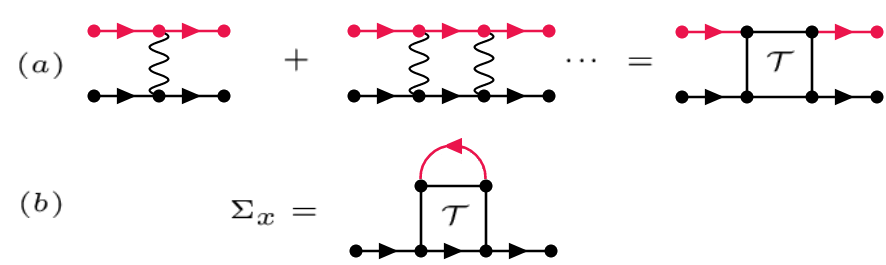
Figure 1: (a) Ladder approximation and the $\mathcal{T}$-matrix. Solid black (red) lines correspond to exciton (electron) propagators and wavy lines represent bare exciton-electron interaction vertices $g_{ex}$ (b) Exciton self-energy $\Sigma_{x}$.

We employ a diagrammatic approach based on the $\mathcal{T}$-matrix, that takes into account the underlying trion-state. The self-energy for the excitons $\Sigma_{x}(\textbf{k},i\omega_{n})$ within the $\mathcal{T}$-matrix approximation is depicted in Fig.1(b), and given explicitly by

$$\Sigma_{x}(\textbf{k},i\omega_{n})=\frac{1}{\beta}\int\frac{d^{2}\textbf{q}}{(2\pi)^{2}}\sum_{iq_{n}}\mathcal{G}^{0}_{e}(\textbf{q},iq_{n})\mathcal{T}(\textbf{k}+\textbf{q},i\omega_{n}+iq_{n}).$$ (7)

Here $i\omega_{n}$ are now bosonic Matsubara frequencies. As we are considering the single exciton-impurity limit, $\Sigma_{x}$ simply reads

$$\Sigma_{x}(\textbf{k},i\omega_{n})=\int\frac{d^{2}\textbf{q}}{(2\pi)^{2}}n_{F}(\epsilon_{\textbf{q}}^{(e)})\mathcal{T}(\textbf{k}+\textbf{q},i\omega_{n}+\epsilon_{\textbf{q}}^{(e)}).$$ (8)

The full Green’s function for excitons is then $\mathcal{G}_{x}^{-1}(\textbf{k},i\omega_{n})=z-\epsilon^{(x)}_{\textbf{k}}-\Sigma_{x}(\textbf{k},i\omega_{n})$. By computing the energy poles of $\mathcal{G}_{x}$, one finds that $\Sigma_{x}$ gives rise to the attractive and repulsive Fermi-polaron states in the absence of light Bastarrachea-Magnani et al. (2020), in a similar fashion as in Fermi gases Massignan et al. (2014); Schmidt et al. (2012). The cavity photon field then couples to the polaron states giving rise to three exciton polaron-polariton branches as it is shown in Fig. 2(a) of the main text.

The emergence of exciton polaron-polaritons can be studied with the $2\times 2$ Green’s function describing both excitonic and photonic degrees of freedom. More precisely, we define $\mathcal{G}(\textbf{k},\tau)=-\left\langle T_{\tau}\left\{\hat{\Psi}_{\textbf{k}}(\tau)\hat{\Psi}^{\dagger}_{\textbf{k}}(0)\right\}\right\rangle$, where $\hat{\Psi}_{\textbf{k}}^{\dagger}\equiv\begin{bmatrix}\hat{x}_{\textbf{k}}^{\dagger}&\hat{c}_{\textbf{k}}^{\dagger}\end{bmatrix}$ and $T_{\tau}$ is the imaginary time-ordering operator. In the frequency space, we have Bastarrachea-Magnani et al. (2020)

$$\mathcal{G}^{-1}(\textbf{k},i\omega_{n})=\begin{bmatrix}i\omega_{n}-\epsilon^{(x)}_{\textbf{k}}-\Sigma_{x}(\textbf{k},i\omega_{n})&-\Omega\\ -\Omega&i\omega_{n}-\epsilon^{(c)}_{\textbf{k}}\end{bmatrix},$$ (9)

which is the form used in the main text.

II Non-equilibrium Bose condensation and Bogoliubov theory

In this section, we provide details on the derivation of the non-equilibrium Gross-Pitaevskii equation (GPE) and the Bogoliubov equations giving the excitation spectrum. To treat the incoherent decay terms of polaritons correctly, we deploy a formalism where the bosonic polariton modes are coupled to an external thermal reservoir bath of harmonic oscillators Meystre and Sargent III (2007); Scully and Zubairy (1997). The role of the reservoir is to take into account the open quantum system nature of the polaron-polariton setup. By assuming that the correlation times of the bath are much smaller than any relevant time scale of the polariton system, i.e. by employing a Markovian approximation, one ends up with the equations of motion which describe the decay of the polaritons.

We emphasize that the right form for the non-equilibrium Green’s function can not be obtained with a non-hermitian decay Hamiltonian of the form $H_{decay}=\sum_{\textbf{k}}i\gamma\hat{b}^{\dagger}_{\textbf{k}}\hat{b}_{\textbf{k}}$, where $\hat{b}_{\textbf{k}}$ is the annihilation operator for the polaron-polariton state at k. This can be seen from the Heisenberg equation of motion which yields $\frac{d\hat{b}_{\textbf{k}}}{dt}=-i[\hat{b}_{\textbf{k}},H_{decay}]=-\gamma\hat{b}_{\textbf{k}}$ but $\frac{d\hat{b}^{\dagger}_{\textbf{k}}}{dt}=\gamma\hat{b}^{\dagger}_{\textbf{k}}$. The solutions for these differential equations give a damping solution for $\hat{b}_{\textbf{k}}$ but an unphysical amplifying solution for $\hat{b}^{\dagger}_{\textbf{k}}$. This inevitably leads to a wrong non-equilibrium theory. Below, we derive the Bogoliubov theory accounting correctly for the losses of the polaron-polaritons, preventing unphysical amplifications of the bosonic fields.

We start by writing down the effective Hamiltonian for the lower polaron-polaritons in the presence an external coherent driving field and incoherent losses:

$$H_{L}=H_{s}+H_{r}+H_{sr},\textrm{ where}$$

$$H_{s}=\sum_{\textbf{k}}\epsilon_{\textbf{k}}\hat{b}^{\dagger}_{\textbf{k}}\hat{b}_{\textbf{k}}+\frac{g}{2A}\sum_{\textbf{k},\textbf{k}^{\prime},\textbf{q}}\hat{b}^{\dagger}_{\textbf{k}}\hat{b}^{\dagger}_{\textbf{k}^{\prime}}\hat{b}_{\textbf{k}^{\prime}-\textbf{q}}\hat{b}_{\textbf{k}+\textbf{q}}+iF_{\textrm{pu}}e^{-i\epsilon_{\textrm{pu}}t}b^{\dagger}_{\textbf{k}_{\textrm{pu}}},$$

$$H_{r}=\sum_{j}\epsilon^{B}_{j}\hat{r}_{j}^{\dagger}\hat{r}_{j}$$

$$H_{sr}=\sum_{\textbf{k},j}\big{[}\kappa_{j}^{*}\hat{b}^{\dagger}_{\textbf{k}}\hat{r}_{j}+\kappa_{j}\hat{r}^{\dagger}_{j}\hat{b}_{\textbf{k}}\big{]}.$$ (10)

Here the polaron-polaritons are described by the system Hamiltonian $H_{s}$, the reservoir bath is $H_{r}$ and the coupling between the system and the bath is treated via $H_{sr}$. The polaron-polariton energies are denoted by $\epsilon_{\textbf{k}}$, $A$ is the system area, $g$ is the effective interaction between polaron-polaritons, $F_{\textrm{pu}}$ is the strength of the laser pump, $\epsilon_{\textrm{pu}}$ is the pump energy and $\textbf{k}_{\textrm{pu}}$ is the in-plane momentum of the pump ($\hbar=1$). In $H_{r}$, $\hat{r}_{j}$ are the annihilation operators for the $j$th reservoir mode of energy $\epsilon^{B}_{j}$. In $H_{sr}$ we have employed the Rotating Wave Approximation (RWA) by assuming that the bandwidth of the bath is much larger than the system-reservoir coupling $\kappa_{j}$ such that the non-energy-conserving terms have been discarded in $H_{sr}$.

By writing down the Heisenberg equation of motions for $\hat{b}_{\textbf{k}}$ and $\hat{r}_{j}$, and deploying the Markovian approximation for the system-reservoir coupling Meystre and Sargent III (2007); Scully and Zubairy (1997), we obtain, after a straightforward algebra, the following

$$i\frac{\partial\hat{b}_{\textbf{k}}}{\partial t}=(\epsilon_{\textbf{k}}-i\gamma)\hat{b}_{\textbf{k}}+iF_{\textrm{pu}}e^{-i\epsilon_{\textrm{pu}}t}\delta_{\textbf{k},\textbf{k}_{\textrm{pu}}}+\big{[}\hat{b}_{\textbf{k}},\frac{g}{2A}\sum_{\textbf{k},\textbf{k}^{\prime},\textbf{q}}\hat{b}^{\dagger}_{\textbf{k}}\hat{b}^{\dagger}_{\textbf{k}^{\prime}}\hat{b}_{\textbf{k}^{\prime}-\textbf{q}}\hat{b}_{\textbf{k}+\textbf{q}}\big{]},$$ (11)

where the polaron-polariton decay is $\gamma=2\pi|\kappa(\epsilon_{\textbf{k}})|^{2}\mathcal{D}(\epsilon_{\textbf{k}})$ with $\kappa(\epsilon)$ being a continuous interpolation of $\kappa_{j}$ and $\mathcal{D}(\epsilon)$ the density of the states of the reservoir Scully and Zubairy (1997). The microscopic details of the reservoir are not important and thus for $\gamma$ we pick an experimentally realistic value of $\gamma=0.4$ meV. Moreover, we have ignored for simplicity the quantum noise term arising from the system-reservoir coupling.

For the purpose of this work, we choose $\textbf{k}_{\textrm{pu}}=0$. Now we assume that the polaron-polariton state at $\textbf{k}_{\textrm{pu}}$ acquires a macroscopic population due to the pump. We therefore approximate $\hat{b}_{\textbf{k}_{\textrm{pu}}}$ as a complex number such that $\hat{b}_{\textbf{k}_{\textrm{pu}}}\approx\sqrt{A}\Psi_{0}(t)$, where $\Psi_{0}(t)$ is the condensation wave function. At the Gross-Pitaevskii mean-field level, the contribution of states of $\textbf{k}\neq\textbf{k}_{\textrm{pu}}$ is neglected and from Eq. (11) we obtain for the condensed state the following:

$$i\partial\Psi_{0}(t)=(\epsilon_{0}-i\gamma)\Psi_{0}(t)+iF_{\textrm{pu}}e^{-i\epsilon_{\textrm{pu}}t}+g|\Psi_{0}(t)|^{2}\Psi_{0}(t),$$ (12)

where $\epsilon_{0}\equiv\epsilon_{\textbf{k}=0}$. By assuming that the condensate wave function follows the time dependence of the driving field, i.e. $\Psi_{0}(t)=\Psi_{0}e^{-i\epsilon_{\textrm{pu}}t}$, one acquires the non-equilibrium Gross-Pitaevsii equation:

$$\epsilon_{\textrm{pu}}\Psi_{0}=(\epsilon_{0}-i\gamma)\Psi_{0}+iF_{\textrm{pu}}+g|\Psi_{0}|^{2}\Psi_{0},$$ (13)

which is the same as Eq. (6) in the main text.

The condensation wave function can be written as $\Psi_{0}=\sqrt{n_{0}}e^{i\phi_{0}}$, where $n_{0}$ is the condensation density. In case of an equilibrium condensate, any value of $\phi_{0}$ would yield the same ground state energy and equally well provide a solution for the equilibrium GPE. However, it turns out that the non-equilibrium GPE of Eq. (13) can be solved in general only for some specific value of $\phi_{0}$, i.e. the external pumping breaks explicitly the $U(1)$ phase symmetry by picking a definite complex phase $\phi_{0}$ for the condensation wave function.

Now we study the excitation spectrum of the non-equilibrium condensate. To this end, we write $\hat{b}_{\textbf{k}}$ as

$$\hat{b}_{\textbf{k}}=\big{[}\sqrt{A}\Psi_{0}\delta_{\textbf{k},0}+\delta\hat{b}_{\textbf{k}}(t)\big{]}e^{-i\epsilon_{\textrm{pu}}t},$$ (14)

where we have introduced the fluctuation term on top of the condensate, $\delta\hat{b}_{\textbf{k}}(t)$, to account for the non-condensed polaron-polaritons. To describe the fluctuations, we introduce the bosonic Green’s function which in the imaginary-time domain reads

$$\mathcal{G}_{B}(\textbf{k},\tau)\equiv-\langle T_{\tau}\begin{bmatrix}\delta\hat{b}_{\textbf{k}}(\tau)\\ \delta\hat{b}^{\dagger}_{-\textbf{k}}(\tau)\end{bmatrix}\begin{bmatrix}\delta\hat{b}^{\dagger}_{\textbf{k}}(0)&\delta\hat{b}_{-\textbf{k}}(0)\end{bmatrix}\rangle=\begin{bmatrix}-\langle T_{\tau}\delta\hat{b}_{\textbf{k}}(\tau)\delta\hat{b}^{\dagger}_{\textbf{k}}(0)\rangle&-\langle T_{\tau}\delta\hat{b}_{\textbf{k}}(\tau)\delta\hat{b}_{-\textbf{k}}(0)\rangle\\ -\langle T_{\tau}\delta\hat{b}^{\dagger}_{-\textbf{k}}(\tau)\delta\hat{b}^{\dagger}_{\textbf{k}}(0)\rangle&-\langle T_{\tau}\delta\hat{b}^{\dagger}_{-\textbf{k}}(\tau)\delta\hat{b}_{-\textbf{k}}(0)\rangle,\end{bmatrix}$$ (15)

where $\textbf{k}\neq 0$ as we are considering the non-condensed polaron-polaritons only. In the Matsubara frequency space one has the Dyson equation Fetter and Walecka (1971):

$$\mathcal{G}_{B}^{-1}(\textbf{k},i\omega_{n})=\mathcal{G}_{B,0}^{-1}(\textbf{k},i\omega_{n})-\Sigma_{B}(\textbf{k},i\omega_{n}).$$ (16)

Here $\Sigma_{B}$ is the self-energy arising from finite interactions between polaron-polaritons and $\mathcal{G}_{B,0}$ is the non-interacting Green’s function, i.e. in the absence of interactions, $g=0$, one has $\mathcal{G}_{B}=\mathcal{G}_{B,0}$.

To proceed, we first evaluate $\mathcal{G}_{B,0}$. We denote the Hamiltonian without the interactions as $H_{0}\equiv H_{L}(g=0)$. Then, by using the Markovian approximation and ignoring the quantum noise terms, we obtain the following imaginary-time equations of motion Meystre and Sargent III (2007); Scully and Zubairy (1997):

$$[\delta\hat{b}_{\textbf{k}}(\tau)e^{\epsilon_{\textrm{pu}}\tau},H_{0}]=(-\epsilon_{\textbf{k}}+i\gamma)\delta\hat{b}_{\textbf{k}}(\tau)e^{\epsilon_{\textrm{pu}}\tau}$$

$$[\delta\hat{b}^{\dagger}_{\textbf{k}}(\tau)e^{-\epsilon_{\textrm{pu}}\tau},H_{0}]=(\epsilon_{\textbf{k}}+i\gamma)\delta\hat{b}^{\dagger}_{\textbf{k}}(\tau)e^{-\epsilon_{\textrm{pu}}\tau}.$$ (17)

The latter equation would have a wrong form for the decay part if we had used the non-hermitian form $H_{decay}=\sum_{\textbf{k}}i\gamma\hat{b}^{\dagger}_{\textbf{k}}\hat{b}_{\textbf{k}}$ describing the decay instead of the system-reservoir formalism. Now, it is straightforward to take the time derivative of $\mathcal{G}_{B,0}(\textbf{k},\tau)$ to show that

$$\partial_{\tau}[\mathcal{G}_{B,0}(\textbf{k},\tau)]_{11}=-\delta(\tau)-(\epsilon_{\textbf{k}}-i\gamma-\epsilon_{\textrm{pu}})[\mathcal{G}_{B,0}(\textbf{k},\tau)]_{11}$$

$$\partial_{\tau}[\mathcal{G}_{B,0}(\textbf{k},\tau)]_{22}=\delta(\tau)+(\epsilon_{\textbf{k}}+i\gamma-\epsilon_{\textrm{pu}})[\mathcal{G}_{B,0}(\textbf{k},\tau)]_{22}.$$ (18)

By transforming these expressions to the Matsubara frequency space, one has

$$\mathcal{G}_{B,0}^{-1}(\textbf{k},z)=\begin{bmatrix}z-\tilde{\epsilon}_{\textbf{k}}+i\gamma&0\\ 0&-z-\tilde{\epsilon}_{\textbf{k}}-i\gamma\end{bmatrix},$$ (19)

where $\tilde{\epsilon}_{\textbf{k}}\equiv\epsilon_{\textbf{k}}-\epsilon_{\textrm{pu}}$.

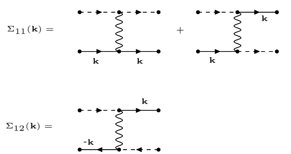
Figure 2: Self-energy diagrams included in the Bogoliubov approximation. The solid propagators are the non-condensed polaron-polaritons, whereas the dashed lines depict polaron-polaritons propagating into and out of the condensate with the wavefunction $\Psi=\sqrt{n_{0}}e^{i\phi_{0}}$. The wavy lines depict the interaction polariton interaction $g$.

The self-energy $\Sigma_{B}$ can be in general evaluated with the diagrammatic Beliaev theory Fetter and Walecka (1971). Here, we deploy the first order Beliaev theory, i.e. the Bogoliubov theory that includes only the diagrams presented in Fig. 2. Since we are interested on low-energy states, for simplicity for the scattering between two polaritons with momenta $\mathbf{k}$ and $\mathbf{k}^{\prime}$ that exchange a momentum q, we approximate the polariton-polariton interactions by $g_{\mathbf{k},\mathbf{k}^{\prime};\mathbf{q}}=g=g_{xx}\tilde{C}(\mathbf{k}=0)^{4}Z^{2}(\mathbf{k}=0)$, and based on the same argument, we assume a momentum independent damping rate $\gamma$. Then the Bogoliubov self-energy reads as

$$\Sigma_{B}=\begin{bmatrix}2gn_{0}&gn_{0}e^{i2\phi_{0}}\\ gn_{0}e^{-i2\phi_{0}}&2gn_{0}\end{bmatrix}.$$ (20)

By inserting the expressions (19) and (20) to the Dyson equation of Eq. (16), one finally obtains the Bogoliubov Green’s function used in the main text:

$$\mathcal{G}_{B}^{-1}(\textbf{k},z)=\begin{bmatrix}z-\tilde{\epsilon}_{\textbf{k}}+i\gamma-2gn_{0}&-gn_{0}e^{i2\phi_{0}}\\ -gn_{0}e^{-i2\phi_{0}}&-z-\tilde{\epsilon}_{\textbf{k}}-i\gamma-2gn_{0}.\end{bmatrix}$$ (21)

Excitation spectrum is then given by $\det[\mathcal{G}_{B}^{-1}(\textbf{k},E_{\textbf{k}})]=0$, yielding the dispersion relation written down in the main text. As the complex phase of condensation wave function, $\phi_{0}$, does not affect the excitation spectrum or the stability condition, $\imaginary[E_{\textbf{k}}]<0$, we have in the main text for simplicity set $\phi_{0}=0$ in the expression of $\mathcal{G}_{B}^{-1}(\textbf{k},z)$.

III Origin of non-linear features

In this section we point out the origin of two different non-linear regimes seen in the low and high electron density limits presented in Fig. 1(c) of the main text. We specifically show that the non-linear feature in the low-$\epsilon_{F}$ regime arises predominantly from the increasing blue detuning of the laser, i.e. $\epsilon_{\textrm{pu}}-\epsilon_{0}$, as a function of increasing $\epsilon_{F}$, whereas the high-$\epsilon_{F}$ non-linear feature results in from the interplay of both increasing $\epsilon_{\textrm{pu}}-\epsilon_{0}$ and $g$ as a function of the electron density.

To demonstrate these claims, we performed two computations: one with fixed $\epsilon_{0}$ and one with fixed $g$ such that in both the computations either only $\epsilon_{0}$ or $g$ was allowed to change as a function of $\epsilon_{F}$. The results are shown in Fig. 3: in Fig. 3(a) we show $n_{0}$ as a function of $\epsilon_{F}$ by fixing the interaction $g$, whereas in Fig. 3(b) the polaron-polariton ground state energy $\epsilon_{0}$ is held fixed. The pump intensity and frequency are the same as in Fig. 1(c) of the main text. In Fig. 3(a) [Fig. 3(b)] the value of interaction $g$ (ground state energy $\epsilon_{0})$ is given by the lowest value of $\epsilon_{F}$, i.e. $g/g_{xx}=0.0029$ ($\epsilon_{0}/2\Omega=0.023$).

From Fig. 3(a) one observes that despite having a constant value for $g$, a non-linear behavior of three solutions can still be produced at the low-$\epsilon_{F}$ regime, in a similar fashion as in Fig. 1(c) of the main text. In contrast, with fixed $\epsilon_{0}$ this feature is absent, see Fig. 3(b). As a consequence, the non-linear behavior seen at the low-$\epsilon_{F}$ regime in Fig. 1(c) of the main text arises due to the modification of $\epsilon_{0}$ as a function of $\epsilon_{F}$.

From Fig. 3(a) we also see that for fixed $g$ one cannot obtain a non-linear behavior at larger $\epsilon_{F}$, in contrast to the feature seen in Fig. 1(c) of the main text. Furthermore, the non-linearity is also absent with fixed $\epsilon_{0}$, see Fig. 3(b). We can thus conclude that the non-linear behavior at the high-$\epsilon_{F}$ regime in Fig. 1(c) of the main text arises because both $\epsilon_{0}$ and $g$ depend strongly on the electron density. Thus, such a non-linear feature cannot be achieved by simply tuning the pump energy in the absence of the 2DEG.

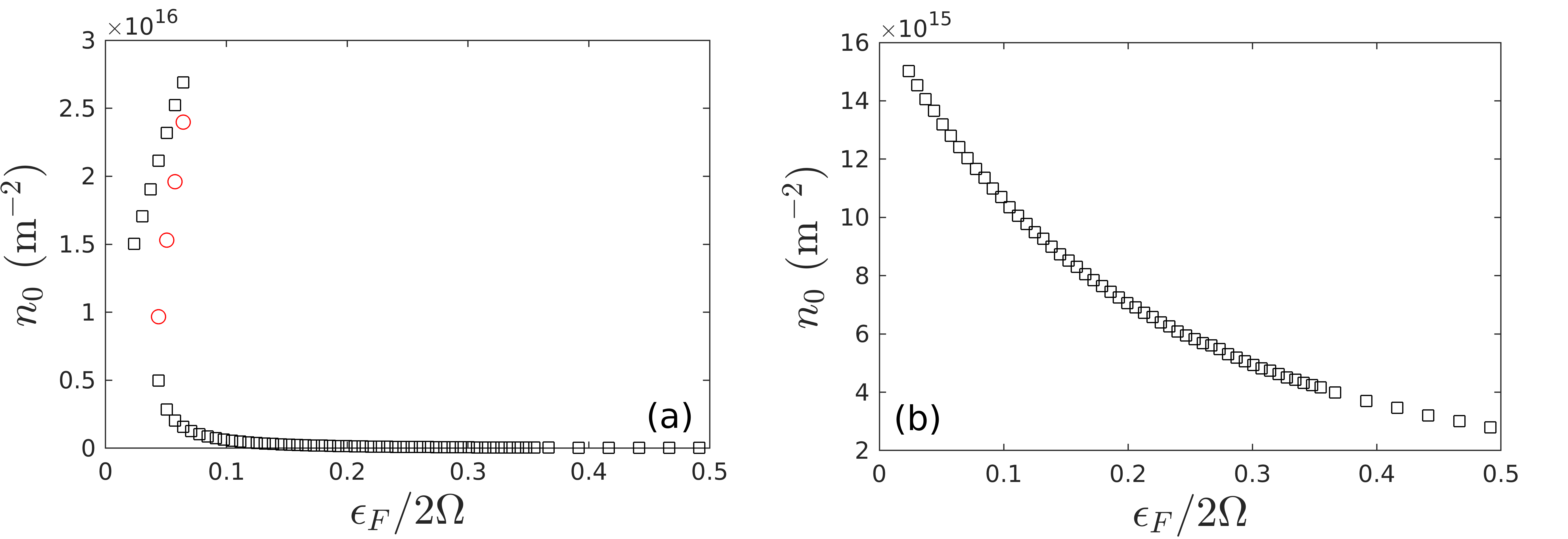
Figure 3: (a) Condensate density $n_{0}$ as a function of electron density for fixed $g(\epsilon_{F}/2\Omega=0.023)/g_{xx}=0.0029$. (b) Condensate density $n_{0}$ as a function of electron density for fixed $\epsilon_{0}(\epsilon_{F}/2\Omega=0.023)/2\Omega=-2.224$. Black square (red dots) indicate stable (unstable) solutions for the non-equilibrium GPE. The pump intensity and energy are the same as in Figs.1(b)-(c) of the main text.

References

• Fetter and Walecka (1971) A. Fetter and J. Walecka, Quantum Theory of Many-Particle Systems, Dover Books on Physics Series (Dover Publications, 1971).
• Bastarrachea-Magnani et al. (2019) M. A. Bastarrachea-Magnani, A. Camacho-Guardian, M. Wouters,  and G. M. Bruun, Phys. Rev. B 100, 195301 (2019).
• Randeria et al. (1990) M. Randeria, J.-M. Duan,  and L.-Y. Shieh, Phys. Rev. B 41, 327 (1990).
• Sidler et al. (2016) M. Sidler, P. Back, O. Cotlet, A. Srivastava, T. Fink, M. Kroner, E. Demler,  and A. Imamoglu, Nature Physics 13, 255 EP (2016).
• Mak et al. (2012) K. F. Mak, K. He, C. Lee, G. H. Lee, J. Hone, T. F. Heinz,  and J. Shan, Nature Materials 12, 207 EP (2012).
• Tan et al. (2020) L. B. Tan, O. Cotlet, A. Bergschneider, R. Schmidt, P. Back, Y. Shimazaki, M. Kroner,  and A. m. c. İmamoğlu, Phys. Rev. X 10, 021011 (2020).
• Bastarrachea-Magnani et al. (2020) M. A. Bastarrachea-Magnani, A. Camacho-Guardian,  and G. M. Bruun, “Attractive and repulsive exciton-polariton interactions mediated by an electron gas,”  (2020), arXiv:2008.10303 [cond-mat.mes-hall] .
• Massignan et al. (2014) P. Massignan, M. Zaccanti,  and G. M. Bruun, Reports on Progress in Physics 77, 034401 (2014).
• Schmidt et al. (2012) R. Schmidt, T. Enss, V. Pietilä,  and E. Demler, Phys. Rev. A 85, 021602 (2012).
• Meystre and Sargent III (2007) P. Meystre and M. Sargent III, Elements of Quantum Optics (Springer-Verlag, 2007).
• Scully and Zubairy (1997) M. Scully and M. Zubairy, Quantum Optics (Cambridge University Press, 1997).