Closed geodesics with prescribed intersection numbers

Abstract.

Let $(\Sigma,g)$ be a closed, oriented, negatively curved surface, and fix pairwise disjoint simple closed geodesics $\gamma_{\star,1},\dots\gamma_{\star,r}$. We give an asymptotic growth as $L\to+\infty$ of the number of primitive closed geodesic of length less than $L$ intersecting $\gamma_{\star,j}$ exactly $n_{j}$ times, where $n_{1},\dots,n_{r}$ are fixed nonnegative integers. This is done by introducing a dynamical scattering operator associated to the surface with boundary obtained by cutting $\Sigma$ along $\gamma_{\star,1},\dots,\gamma_{\star,r}$ and by using the theory of Pollicott-Ruelle resonances for open systems.

1. Introduction

Let $(\Sigma,g)$ be a closed oriented negatively curved Riemannian surface and denote by $\mathcal{P}$ the set of its oriented primitive closed geodesics. For $L>0$ define

$$N(L)=\#\{\gamma\in\mathcal{P},\leavevmode\nobreak\ \ell(\gamma)\leqslant L\},$$

where $\ell(\gamma)$ is the length of a geodesic $\gamma$. Then a classical result obtained by Margulis [Mar69] states that

$$N(L)\sim\frac{\mathrm{e}^{hL}}{hL}$$

as $L\to+\infty$, where $h>0$ is the topological entropy of the geodesic flow of $(\Sigma,g)$.

The purpose of this paper is to understand the asymptotic behavior of the quantity

$$N(\mathbf{n},L)=\#\left\{\gamma\in\mathcal{P},\leavevmode\nobreak\ \ell(\gamma)\leqslant L,\leavevmode\nobreak\ i(\gamma,\gamma_{\star,j})=n_{j},\leavevmode\nobreak\ j=1,\dots,r\right\}$$

as $L\to+\infty$, where $\gamma_{\star,1},\dots,\gamma_{\star,r}$ are some pairwise disjoint simple closed geodesics, $\mathbf{n}=(n_{1},\dots,n_{r})\in\mathbb{N}^{r}$, and $i(\gamma,\gamma_{\star_{j}})$ is the geometric intersection number between $\gamma$ and $\gamma_{\star,j}$. The main result goes as follows.

Theorem 1.

Let $\mathbf{n}=(n_{1},\dots,n_{r})\in\mathbb{N}^{r}$. If $N(\mathbf{n},L)>0$ for some $L>0$, then there are $C_{\mathbf{n}}>0,d_{\mathbf{n}}\in\mathbb{N}$ and $h_{\mathbf{n}}\in]0,h[$ such that

$$N(\mathbf{n},L)\sim C_{\mathbf{n}}L^{d_{\mathbf{n}}-1}\mathrm{e}^{h_{\mathbf{n}}L},\quad L\to+\infty.$$

In fact, a similar statement holds if we aditionnaly prescribe the order in which we want the intersections to occur, as follows. Let us denote by $\Sigma_{1},\dots,\Sigma_{q}$ the connected components of the surface $\Sigma_{\star}=\Sigma\setminus(\gamma_{\star,1}\cup\cdots\cup\gamma_{\star,r})$ obtained by cutting $\Sigma$ along $\gamma_{\star,1},\dots,\gamma_{\star,r}$. Let $\gamma\in\mathcal{P}$ intersecting at least one $\gamma_{\star,i}$. For each $\gamma\in\mathcal{P}$, we denote by $\omega(\gamma)$ the pair $(u,v)$ of cyclically ordered sequences $u=(u_{1},\dots,u_{N})$ and $v=(v_{1},\dots,v_{N})$ such that $\gamma$ goes through $\Sigma_{v_{1}},\dots,\Sigma_{v_{N}}$ (in this order) and passes from $\Sigma_{v_{k}}$ to $\Sigma_{v_{k+1}}$ by crossing $\gamma_{\star,u_{k}}$, where $v_{N+1}=v_{1}$ (see Figure 1) ; those sequence are well defined modulo cyclic permutations. Any pair of finite sequences $\omega$ will be called an admissible path if $\omega\sim\omega(\gamma)$ for some $\gamma\in\mathcal{P}$, where $\omega\sim\omega(\gamma)$ means that $\omega(\gamma)$ is a cyclic permutation of $\omega$ (the permutation being the same for both components of $\omega$).

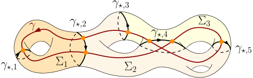
Figure 1. A closed geodesic $\gamma$ on $\Sigma$. Here we have $r=5$, $q=3$, and $\omega(\gamma)\sim(u,v)$ where $u=(1,2,4,5,4,3,2)$ and $v=(1,1,2,3,2,3,2)$ (the starting point of $\gamma$ is the red arrow).

Denote by $S\Sigma$ the unit tangent bundle of $(\Sigma,g)$ and by $(\varphi_{t})_{t\in\mathbb{R}}$ the associated geodesic flow, acting on $S\Sigma$. Let $\pi:S\Sigma\to\Sigma$ be the natural projection. We denote by $h_{j}>0$ ($j=1,\dots,q$) the entropy of the open system $(\Sigma_{j},g|_{\Sigma_{j}})$, that is, the topological entropy of the flow $\varphi$ restricted to the trapped set

$$K_{j}=\overline{\{(x,v)\in S\Sigma,\leavevmode\nobreak\ \pi(\varphi_{t}(x,v))\in\Sigma_{j},\leavevmode\nobreak\ t\in\mathbb{R}\}}$$

where the closure is taken in $S\Sigma$.

For any admissible path $\omega=(u,v)$ of length $N$, we set

$$h_{\omega}=\max\{h_{v_{k}},\leavevmode\nobreak\ k=1,\dots,N\},\quad d_{\omega}=\#\{k=1,\dots,N,\leavevmode\nobreak\ h_{v_{k}}=h_{\omega}\}.$$

The number $h_{\omega}$ is the maximum of the entropies of the surfaces encountered by any $\gamma\in\mathcal{P}$ satisfying $\omega(\gamma)\sim\omega$, while $d_{\omega}$ is the number of times any such $\gamma$ will encounter a surface whose entropy is equal to $h_{\omega}$ (for example, in Figure 1, if the entropy $h_{2}$ of $\Sigma_{2}$ is the greatest, we have $h(\omega)=h_{2}$ and $d(\omega)=3$, as $\gamma$ travels three times through $\Sigma_{2}$).

In fact, the numbers $h_{\omega}$ and $d_{\omega}$ depend only on $\mathbf{n}(\omega)=(n_{1},\dots,n_{r})$ where $n_{j}=\#\{k=1,\dots,N,\leavevmode\nobreak\ u_{k}=j\}$ (see §10) ; we will thus refer to them by $h_{\mathbf{n}(\omega)}$ and $d_{\mathbf{n}(\omega)}$ respectively.

Theorem 2.

Let $\omega$ be an admissible path. Then there is $c(\omega)>0$ such that

$$\#\{\gamma\in\mathcal{P},\leavevmode\nobreak\ \ell(\gamma)\leqslant L,\leavevmode\nobreak\ \omega(\gamma)\sim\omega\}\sim c(\omega)L^{d_{\mathbf{n}(\omega)}-1}\mathrm{e}^{h_{\mathbf{n}(\omega)}L},\quad L\to+\infty.$$

Note that Theorem 1 can be deduced from Theorem 2 by summing over admissible paths $\omega$ with $\mathbf{n}(\omega)=\mathbf{n}$ where $\mathbf{n}\in\mathbb{N}^{r}$ is fixed. We refer to §10 for a slightly more precise statement.

For the sake of simplicity, and to make the exposition clearer, we will deal in the major part of this article with the case $r=1$. The case $r>1$ will be then obtained by identical techniques, as described in §10. Thus from now on and unless stated otherwise, we will assume that we are given only a simple closed geodesic $\gamma_{\star}$ and we set

$$N(n,L)=\#\left\{\gamma\in\mathcal{P},\leavevmode\nobreak\ \ell(\gamma)\leqslant L,\leavevmode\nobreak\ i(\gamma,\gamma_{\star})=n\right\}.$$

In this context, our result reads as follows.

Theorem 3.

Let $\gamma_{\star}$ be a nontrivial simple closed geodesic of $(\Sigma,g).$

1. Suppose that $\gamma_{\star}$ is not separating, that is $\Sigma\setminus\gamma_{\star}$ is connected. Then there exists $c_{\star}>0$ such that for each $n\in\mathbb{N}$,

   $$N(n,L)\sim\frac{(c_{\star}L)^{n}}{n!}\frac{\mathrm{e}^{h_{\star}L}}{h_{\star}L},\quad L\to+\infty,$$

   where $h_{\star}\in]0,h[$ is the entropy of the geodesic flow of the open system $(\Sigma\setminus\gamma_{\star})$.
   

2. Suppose that $\gamma_{\star}$ separates $\Sigma$ in two surfaces $\Sigma_{1}$ and $\Sigma_{2}$. Let $h_{j}\in]0,h[$ denote the entropy of the open system $(\Sigma_{j},g|_{\Sigma_{j}})$ and set $h_{\star}=\max(h_{1},h_{2})$. Then there is $c_{\star}>0$ such that for each $n\in\mathbb{N}$ we have as $L\to+\infty,$

   $$N(2n,L)\sim\left\{\begin{matrix}\displaystyle{\frac{(c_{\star}L)^{n}}{n!}\frac{\mathrm{e}^{h_{\star}L}}{h_{\star}L}}\quad&\text{ if }h_{1}\neq h_{2},\vspace{0.3cm}\\ \displaystyle{2\frac{\left(c_{\star}L^{2}\right)^{n}}{(2n)!}\frac{\mathrm{e}^{h_{\star}L}}{h_{\star}L}}\quad&\text{ if }\leavevmode\nobreak\ h_{1}=h_{2},\end{matrix}\right.$$

As before, the entropy $h_{\star}$ is defined as the topological entropy of the geodesic flow restricted to the trapped set

$$K_{\star}=\overline{\{(x,v)\in S\Sigma,\leavevmode\nobreak\ \pi(\varphi_{t}(x,v))\in\Sigma\setminus\gamma_{\star}\leavevmode\nobreak\ t\in\mathbb{R}\}}$$

where the closure is taken in $S\Sigma$.

Remark 1.1.

1. The case $n=0$ is well known and follows from the growth rate of periodic orbits of Axiom A flows obtained by Parry-Pollicott [PP83] (see §2.4). However, to the best of our knowledge, the result is new for $n>0$.

2. Using a classical large deviation result by Kifer [Kif94] and Bonahon’s intersection form [Bon86], we are in fact able to show that a typical closed geodesic $\gamma$ satisfies $i(\gamma,\gamma_{\star})\approx I_{\star}\ell(\gamma)$ for some $I_{\star}>0$ not depending on $\gamma$ (see Proposition 9.1 below for a precise statement). In particular Theorem 3 is a statement about very uncommon closed geodesics.

We also have an equidistribution result, as follows. We still denote by $(\varphi_{t})_{t\in\mathbb{R}}$ the geodesic flow of $(\Sigma,g)$ acting on the unit tangent bundle $S\Sigma$. We set

$$\tilde{\partial}=\{(x,v)\in S\Sigma,\leavevmode\nobreak\ x\in\gamma_{\star}\}\quad\text{and}\quad\Gamma=S\gamma_{\star}\cup\left\{z\in\tilde{\partial},\leavevmode\nobreak\ \varphi_{t}(z)\in S\Sigma\setminus\tilde{\partial},\leavevmode\nobreak\ t>0\right\}$$

where $S\gamma_{\star}=\{(x,v)\in\tilde{\partial},\leavevmode\nobreak\ v\in T_{x}\gamma_{\star}\}.$ We define the Scattering map $S:\tilde{\partial}\setminus\Gamma\to\tilde{\partial}$ by

$$S(z)=\varphi_{\ell(z)}(z),\quad\ell(z)=\inf\{t>0,\leavevmode\nobreak\ \varphi_{t}(z)\in\tilde{\partial}\},\quad z\in\tilde{\partial}\setminus\Gamma.$$

For any $n\in\mathbb{N}_{\geqslant 1}$ we set

$$\Gamma_{n}=\tilde{\partial}\setminus\left\{z\in\tilde{\partial}\setminus\Gamma,\leavevmode\nobreak\ S^{k}(z)\in\tilde{\partial}\setminus\Gamma,\leavevmode\nobreak\ k=1,\dots,\leavevmode\nobreak\ n-1\right\}$$

which is a closed set of Lebesgue measure zero, and

$$\ell_{n}(z)=\ell(z)+\dots+\ell(S^{n-1}(z)),\quad z\in\tilde{\partial}\setminus\Gamma_{n}.$$

Theorem 4.

Let $n\geqslant 1$. For any $f\in C^{\infty}(\tilde{\partial})$ the limit

$$\lim_{L\to+\infty}\frac{1}{nN(n,L)}\sum_{\begin{subarray}{c}\gamma\in\mathcal{P}\\ i(\gamma,\gamma_{\star})=n\end{subarray}}\sum_{z\in I_{\star}(\gamma)}f(z)$$

exists, where for any $\gamma\in\mathcal{P}$, $I_{\star}(\gamma)=\{(x,v)\in S\gamma,\leavevmode\nobreak\ x\in\gamma_{\star}\}$ is the set of incidence vectors of $\gamma$ along $\gamma_{\star}$. This formula defines a probability measure $\mu_{n}$ on $\tilde{\partial}$, whose support is contained in $\Gamma_{n}.$

We will give a full description of $c_{\star}$ and $\mu_{n}$ in terms of Pollicott-Ruelle resonant states of the geodesic flow of $(\Sigma_{\star},g)$ for the resonance $h_{\star}$ in §7. Here $\Sigma_{\star}$ is the compact surface with boundary obtained by cutting $\Sigma$ along $\gamma_{\star}$ (see §2.4).

Strategy of proof

A key ingredient used in the proof of Theorems 3 and 4 is the Scattering operator $\mathcal{S}(s):C^{\infty}(\tilde{\partial})\to C^{\infty}(\tilde{\partial}\setminus\Gamma)$ which is defined by

$$\mathcal{S}(s)f(z)=f(S(z))\mathrm{e}^{-s\ell(z)},\quad z\in\tilde{\partial}\setminus\Gamma,\quad s\in\mathbb{C}.$$

As a first step (which is of independent interest, see Corollary 6), we prove that the family $s\mapsto\mathcal{S}(s)$ extends to a meromorphic family of operators $\mathcal{S}(s):C^{\infty}(\tilde{\partial})\to\mathcal{D}^{\prime}(\tilde{\partial})$ on the whole complex plane (here $\mathcal{D}^{\prime}(\tilde{\partial})$ denotes the space of distributions on $\tilde{\partial}$), whose poles are contained in the set of Pollicott–Ruelle resonances of the geodesic flow of the surface with boundary $(\Sigma_{\star},g)$ (see §2.5 for the definition of those resonances). In this context, the existence of such resonances follows from the work of Dyatlov–Guillarmou [DG16]. By using the microlocal structure of the resolvent of the geodesic flow provided by [DG16], we are moreover able to prove that for any $\chi\in C^{\infty}_{c}(\tilde{\partial}\setminus S\gamma_{\star})$, the composition $(\chi\mathcal{S}(s))^{n}$ is well defined for any $n\geqslant 1$, as well as its super flat trace (meaning that we also look at the action of $\mathcal{S}(s)$ on differential forms, see §3.4) which reads

$${\operatorname{tr}}_{\mathrm{s}}^{\flat}[(\chi\mathcal{S}(s))^{n}]=n\sum_{i(\gamma,\gamma_{\star})=n}\frac{\ell^{\#}(\gamma)}{\ell(\gamma)}\mathrm{e}^{-s\ell(\gamma)}\prod_{z\in I_{\star}(\gamma)}\chi(z),$$

where the products runs over all closed geodesics (not necessarily primitive) $\gamma$ with $i(\gamma,\gamma_{\star})=n$ and $\ell^{\#}(\gamma)$ is the primitive length of $\gamma$ ; this formula is a consequence of the Atiyah-Bott trace formula [AB67]. Furthermore, using a priori bounds on the growth of $N(n,L)$ (obtained in §4), we prove that $s\mapsto{\operatorname{tr}}_{\mathrm{s}}^{\flat}[(\chi\mathcal{S}(s))^{n}]$ has a pole of order $n$ at $s=h$, provided that $\chi$ has enough support. Then letting the support of $1-\chi$ being very close to $S\gamma_{\star}$, and estimating the growth of geodesics intersecting $n$ times $\gamma_{\star}$ with at least one small angle, we are able to derive Theorem 3 from a classical Tauberian theorem of Delange [Del54].

Application to geodesic billards

We finally state a result on the growth number of periodic trajectories of the billard problem associated to a negatively curved surface with totally geodesic boundary, which follows from the methods used to prove Theorem 3.

Corollary 5.

Let $(\Sigma^{\prime},g^{\prime})$ be a negatively curved surface with totally geodesic boundary. For any $n\in\mathbb{N}$ and $L>0$ we denote by $N(n,L)$ the number of closed billiard trajectories on $(\Sigma^{\prime},g^{\prime})$ (that is, geodesic trajectories that bounce on $\partial\Sigma^{\prime}$ according to Descartes’ law) with exactly $n$ rebounds, and with length not greater than $L$. Then there is $c^{\prime}>0$ such that

$$N(n,L)\sim\frac{(c^{\prime}L)^{n}}{n!}~\frac{\mathrm{e}^{h^{\prime}L}}{h^{\prime}L},\quad L\to+\infty,$$

where $h^{\prime}$ is the entropy of the open system $(\Sigma^{\prime},g^{\prime})$.

Related works

As mentioned before, the case $n=0$ follows from the work Parry–Pollicott [PP83] which is based on important contributions of Bowen [Bow72, Bow73], as the geodesic flow on $(\Sigma_{\star},g)$ can be seen as an Axiom A flow (see Lemma 2.4 below and [DG16, §6.1]). For counting results on non compact Riemann surfaces, see also Sarnak [Sar80], Guillopé [Gui86], or Lalley [Lal89]. We refer to the work of Paulin–Pollicott–Schapira [PPS12] for counting results in more general settings.

We also mention a result by Pollicott [Pol85] which says that, if $(\Sigma,g)$ is of constant curvature $-1$ and if $\gamma_{\star}$ is not separating,

$$\frac{1}{N(L)}\sum_{\begin{subarray}{c}\gamma\in\mathcal{P}\\ \ell(\gamma)\leqslant L\end{subarray}}i(\gamma,\gamma_{\star})\sim I_{\star}L$$ (1.1)

for some $I_{\star}>0$, which means that, the average intersection number between $\gamma_{\star}$ and geodesics of length not greater than $L$ is about $I_{\star}L$. We show that this also holds in our context (see §9.2).

Lalley [Lal88], Pollicott [Pol91] and Anantharaman [Ana00] investigated the asymptotic growth of the number of closed geodesics satisfying some homological constraints (see also Philips–Sarnak [PS87] and Katsuda–Sunada [KS88] for the constant curvature case). They show that for any homology class $\xi\in H_{1}(\Sigma,\mathbb{Z})$, we have

$$\#\{\gamma\in\mathcal{P},\leavevmode\nobreak\ \ell(\gamma)\leqslant L,\leavevmode\nobreak\ [\gamma]=\xi\}~\sim C\mathrm{e}^{hL}/L^{\mathrm{g}+1}$$

for some $C>0$ independent of $\xi$, where $\mathrm{g}$ is the genus of $\Sigma$ and $h>0$ is the entropy of the geodesic flow of $(\Sigma,g)$. Such asymptotics are obtained by studying $L$-functions associated to some characters of $H_{1}(\Sigma,\mathbb{Z})$. However our problem is very different in nature; indeed, fixing a constraint in homology boils down to fixing algebraic intersection numbers whereas here we are interested in geometric intersection numbers. This makes $L$-funtions not well suited for this situation.

In the context of hyperbolic surfaces, Mirzhakani [Mir08, Mir16] computed the asymptotic growth of closed geodesics with prescribed self intersection numbers. Namely, for any $k\in\mathbb{N}$, we have

$$\#\{\gamma\in\mathcal{P},\leavevmode\nobreak\ \ell(\gamma)\leqslant L,\leavevmode\nobreak\ ~i(\gamma,\gamma)=k\}\sim c_{k}L^{6(\mathrm{g}-1)},$$

where $i(\gamma,\gamma)$ denote the self-intersection number of $\gamma$ (see also [ES16]).

Organization of the paper

The paper is organized as follows. In §2 we introduce some geometrical and dynamical tools. In §3 we introduce the dynamical scattering operator which is a central object in this paper and we compute its flat trace. In §4 we prove a priori bounds on $N(n,L)$. In §5 we use a Tauberian argument to estimate certain quantities. In §6 we prove Theorem 3. In §7 we prove Theorem 4. In §8 we explain how the methods described above apply to the billard problem. In §9 we show that a typical closed geodesic $\gamma$ satisfies $i(\gamma,\gamma_{\star})\approx I_{\star}\ell(\gamma)$ for some $I_{\star}>0.$ Finally in §10 we extend the results to the case where we are given more than one closed geodesic.

Acknowledgements

I am grateful to Colin Guillarmou for a lot of insightful discussions and for his careful reading of many versions of the present article. I also thank Frédéric Paulin for his help concerning the geometrical lemma 4.7. This project has received funding from the European Research Council (ERC) under the European Unions Horizon 2020 research and innovation programme (grant agreement No. 725967).

2. Geometrical preliminaries

We recall here some classical geometrical and dynamical notions, and introduce the Pollicott-Ruelle resonances that arise in our setting.

2.1. Structural equations

Here we recall some classical facts from [ST76, §7.2] about geometry of surfaces. Denote by $M=S\Sigma=\{(x,v)\in T\Sigma,\leavevmode\nobreak\ \|v\|_{g}=1\}$ the unit tangent bundle of $\Sigma$, by $X$ the geodesic vector field on $M$, that is the generator of the geodesic flow $\varphi=(\varphi_{t})_{t\in\mathbb{R}}$ of $(\Sigma,g)$, acting on $M$. We have the Liouville one-form $\alpha$ on $M$ defined by

$$\langle\alpha(z),\eta\rangle=\langle\mathrm{d}_{(x,v)}\pi(\eta),v\rangle,\quad(x,v)\in M,\quad\eta\in T_{(x,v)}M.$$

Then $\alpha$ is a contact form (that is, $\alpha\wedge\mathrm{d}\alpha$ is a volume form on $M$) and it turns out that $X$ is the Reeb vector field associated to $\alpha$, meaning that

$$\iota_{X}\alpha=1,\quad\iota_{X}\mathrm{d}\alpha=0,$$

where $\iota$ denote the interior product.

We also set $\beta=R_{\pi/2}^{*}\alpha$ where for $\theta\in\mathbb{R}$, $R_{\theta}:M\to M$ is the rotation of angle $\theta$ in the fibers; finally we denote by $\psi$ the connection one-form, that is the unique one-form on $M$ satisfying

$$\iota_{V}\psi=1,\quad\mathrm{d}\alpha=\psi\wedge\beta,\quad\mathrm{d}\beta=-\psi\wedge\alpha,$$

where $V$ is the vertical vector field, that is, the vector field generating $(R_{\theta})_{\theta\in\mathbb{R}}$. Then $(\alpha,\beta,\psi)$ is a global frame of $T^{*}M$, and we denote $H$ the vector field on $M$ such that $(X,H,V)$ is the dual frame of $(\alpha,\beta,\psi)$. We then have the commutation relations

$$[V,X]=H,\quad[V,H]=-X,\quad[X,H]=(\kappa\circ\pi)V,$$

where $\kappa$ is the Gauss curvature of $(\Sigma,g)$.

2.2. The Anosov property

It is well known [Ano67] that the flow $(\varphi_{t})$ has the Anosov property, that is, for any $z\in M$, there is a splitting

$$T_{z}M=\mathbb{R}X(z)\oplus E_{s}(z)\oplus E_{u}(z)$$

which depends continuously on $z$, and with the following property. For any norm $\|\cdot\|$ on $TM$, there exists $C,\nu>0$ such that

$$\left\|\mathrm{d}\varphi_{t}(z)v\right\|~\leqslant C\mathrm{e}^{-\nu t}\|v\|~,\quad v\in E_{s}(z),\quad t\geqslant 0,\quad z\in M,$$

and

$$\left\|\mathrm{d}\varphi_{-t}(z)v\right\|~\leqslant C\mathrm{e}^{-\nu t}\|v\|,\quad v\in E_{u}(z),\quad t\geqslant 0,\quad z\in M$$

In fact $E_{s}(z)\oplus E_{u}(z)=\ker\alpha(z)$ and there exists two continuous functions $r_{\pm}:M\to\mathbb{R}$ such that $\pm r_{\pm}>0$ and

$$E_{s}(z)=\mathbb{R}(H(z)+r_{-}V(z)),\quad E_{u}(z)=\mathbb{R}(H(z)+r_{+}V(z)),\quad z\in M.$$

Moreover $r_{\pm}$ satisfy the Ricatti equation

$$\pm Xr_{\pm}+r_{\pm}^{2}+\kappa\circ\pi=0,$$

where $\kappa$ is the curvature of $\Sigma$.

We will denote by $T^{*}M=E_{0}^{*}\oplus E^{*}_{s}\oplus E_{u}^{*}$ the splitting defined by (here the bundle $\mathbb{R}X$ is denoted by $E_{0}$)

$$E_{0}^{*}(E_{u}\oplus E_{s})=0,\quad E_{s}^{*}(E_{s}\oplus E_{0})=0,\quad E_{u}^{*}(E_{u}\oplus E_{0})=0.$$

Then we have $E_{0}^{*}=\mathbb{R}\alpha$ and

$$E_{s}^{*}=\mathbb{R}(r_{-}\beta-\psi),\quad E_{u}^{*}=\mathbb{R}(r_{+}\beta-\psi).$$ (2.1)

Note that this decomposition does not coincide with the usual dual decomposition, but it is motivated by the fact that covectors in $E_{s}^{*}$ (resp. $E_{u}^{*}$) are exponentially contracted in the future (resp. in the past). Also, we will often consider the symplectic lift of $\varphi_{t},$

$$\Phi_{t}(z,\xi)=(\varphi_{t}(z),\leavevmode\nobreak\ \mathrm{d}\varphi_{t}(z)^{-\top}\cdot\xi),\quad(z,\xi)\in T^{*}M,\quad t\in\mathbb{R},$$ (2.2)

where ^-⊤ denotes the inverse transpose. We have the following lemma (see [DR20, §3.2]).

Lemma 2.1.

For any $\pm t>0$ we have $\iota_{V}\Phi_{t}(\beta)\neq 0$ and $\iota_{H}\Phi_{t}(\psi)\neq 0$.

2.3. A nice system of coordinates

In what follows we denote

$$\tilde{\partial}=\{(x,v)\in M,\leavevmode\nobreak\ x\in\gamma_{\star}\}=S\Sigma|_{\gamma_{\star}}.$$

Lemma 2.2.

There exists a tubular neighborhood $U$ of $\tilde{\partial}$ in $M$ and coordinates $(\tau,\rho,\theta)$ on $U$ with

$$U\simeq(\mathbb{R}/\ell_{0}\mathbb{Z})_{\tau}\times(-\delta,\delta)_{\rho}\times(\mathbb{R}/{2\pi\mathbb{Z}})_{\theta},$$

such that

$$|\rho(z)|=\mathrm{dist}_{g}(\pi(z),\gamma_{\star}),\quad S_{z}\Sigma=\{(\tau(z),\rho(z),\theta),\leavevmode\nobreak\ \theta\in\mathbb{R}/2\pi\mathbb{Z}\},\quad z\in U.$$

Moreover in these coordinates, we have, on $\{\rho=0\}$,

$$X=\cos(\theta)\partial_{\tau}+\sin(\theta)\partial_{\rho},\quad H=-\sin(\theta)\partial_{\tau}+\cos(\theta)\partial_{\rho},\quad V=\partial_{\theta},$$

and

$$\alpha=\cos(\theta)\mathrm{d}\tau+\sin(\theta)\mathrm{d}\rho,\quad\beta=-\sin(\theta)\mathrm{d}\tau+\cos(\theta)\mathrm{d}\rho,\quad\psi=\mathrm{d}\theta.$$

Proof.

For $\tau\in\mathbb{R}/\ell_{0}\mathbb{Z}$ we set $(x_{\tau},v_{\tau})=\varphi_{\tau}(\gamma_{\star}(0),\dot{\gamma}_{\star}(0)).$ We now define, for $\delta>0$ small enough,

$$\psi(\tau,\rho,\theta)=R_{\theta-\pi/2}\varphi_{\rho}(x_{\tau},\nu(x_{\tau})),\quad(\tau,\rho,\theta)\in\mathbb{R}/\ell_{0}\mathbb{Z}\times(-\delta,\delta)\times\mathbb{R}/2\pi\mathbb{Z},$$

where $R_{\eta}:S\Sigma\to S\Sigma$ is the rotation of angle $\eta$ and $\nu(x_{\tau})=R_{\pi/2}v_{\tau}$. As $V=\partial_{\theta}$ and $\iota_{V}\alpha=\iota_{V}\beta=0$, we may write $\alpha(\tau,0,\theta)=a(\tau,\theta)\mathrm{d}\tau+b(\tau,\theta)\mathrm{d}\rho$ and $\beta(\tau,0,\theta)=a^{\prime}(\tau,\theta)\mathrm{d}\tau+b^{\prime}(\tau,\theta)\mathrm{d}\rho$ for some smooth functions $a,a^{\prime},b,b^{\prime}$. Now since $\mathrm{d}\alpha=\psi\wedge\beta$ we obtain $\mathcal{L}_{V}\alpha=\iota_{V}\mathrm{d}\alpha=\beta$, and similarly $\mathcal{L}_{V}\beta=-\alpha.$ Thus we obtain $a^{\prime}=\partial_{\theta}a$, $b^{\prime}=\partial_{\theta}b$ and

$$\partial_{\theta}^{2}a+a=0,\quad\partial_{\theta}^{2}b+b=0.$$

In consequence we have $a(\tau,\theta)=a_{1}(\tau)\cos\theta+a_{2}(\tau)\sin\theta$ and $b(\tau,\theta)=b_{1}(\tau)~\cos\theta+b_{2}(\tau)\sin\theta$ for some smooth functions $a_{1},a_{2},b_{1},b_{2}.$ Moreover, by definition of the coordinates $(\tau,\rho,\theta)$, one has

$$X(\tau,0,0)=\partial_{\tau}\quad\text{ and }\quad X(\tau,0,\pi/2)=\partial_{\rho}.$$ (2.3)

Therefore $a_{1}=b_{2}=1$ and $a_{2}=b_{1}=0$. We thus get the desired formulas for $\alpha$ and $\beta$. Now writing $\psi=a^{\prime\prime}\mathrm{d}\tau+b^{\prime\prime}\mathrm{d}\rho+\mathrm{d}\theta$ and using $\mathcal{L}_{V}\psi=0$, we obtain $\partial_{\theta}a^{\prime\prime}=\partial_{\theta}b^{\prime\prime}=0$. As $\iota_{X}\psi=0$ we obtain $a^{\prime\prime}=b^{\prime\prime}=0$ by (2.3). The formulae for $X,H,V$ follow. ∎

Remark 2.3.

If $\partial=\{\rho=0\}$, we get for any $z=(\tau,0,\theta)\in\partial$

$$T_{z}\partial=\mathbb{R}V(z)\oplus\mathbb{R}(\cos(\theta)X(z)-\sin(\theta)H(z)),\quad N^{*}_{z}\partial=\mathbb{R}(\sin(\theta)\alpha(z)+\cos(\theta)\beta(z)).$$

2.4. Cutting the surface along $\gamma_{\star}$

As mentioned in the introduction, we may see $\Sigma\setminus\gamma_{\star}$ as the interior of a compact surface $\Sigma_{\star}$ with boundary consisting of two copies of $\gamma_{\star}$. By gluing two copies of the annulus $U$ obtained in the preceding subsection on each component of the boundary of $\Sigma_{\star}$, we construct a slightly larger surface $\Sigma_{\delta}\supset\Sigma_{\star}$ whose boundary is identified with the boundary of $U$ (see Figure 2).

Lemma 2.4.

The surface $\Sigma_{\delta}$ has strictly convex boundary, in the sense that the second fundamental form of the boundary $\partial\Sigma_{\delta}$ with respect to its outward normal pointing vector is strictly negative.

Proof.

In the coordinates defined $(\tau,\rho)$ given by Lemma 2.2, the metric $g$ has the form

$$\mathrm{d}\rho^{2}+f(\rho)\mathrm{d}\tau^{2},$$ (2.4)

for some $f>0$ satisfying $f^{\prime}(0)=0$ and one can check that the scalar curvature writes $\kappa(\tau,\rho)=-f^{\prime\prime}(\rho)/f(\rho)$. Thus $f^{\prime\prime}>0$ which gives $\pm f^{\prime}(\rho)>0$ if $\pm\rho>0$. Now if $\nabla$ is the Levi-Civita connexion we have

$$-\langle\nabla_{\partial_{\tau}}\partial_{\rho},\partial_{\tau}\rangle=-f(\rho)\Gamma_{\rho\tau}^{\tau}=-f^{\prime}(\rho)/2,$$

which concludes, since $\partial_{\rho}$ is outward pointing (resp. inward pointing) for at $\{\rho=\delta\}$ (resp. $\{\rho=-\delta\}$). ∎

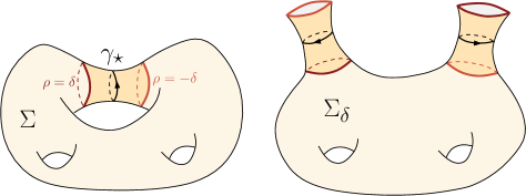
Figure 2. The surfaces $\Sigma$ (on the left) and $\Sigma_{\delta}$ (on the right), in the case where $\gamma_{\star}$ is not separating. In $\Sigma$, the darker region corresponds to the neighborhood $\pi(U)$ of $\gamma_{\star}$.

2.5. The resolvent of the geodesic vector field for open systems

In what follows, we denote by $\Omega^{\bullet}(M_{\delta})$ the set of differential forms on $M_{\delta}$ and by $\Omega^{\bullet}_{c}(M_{\delta})$ the elements of $\Omega^{\bullet}(M_{\delta})$ whose support is contained in the interior of $M_{\delta}$. The set of currents on $M_{\delta}$, denoted by $\mathcal{D}^{\prime\bullet}(M_{\delta})$, is defined as the dual of $\Omega_{c}^{\bullet}(M_{\delta})$ with respect to the pairing

$$(u,v)=\int_{M_{\delta}}u\wedge v,\quad u,v\in\Omega^{\bullet}(M_{\delta}).$$

The geodesic flow $\varphi$ on $M$ induces a flow on $M_{\delta}=S\Sigma_{\delta}$ which we still denote by $\varphi$. We define

$$\ell_{\pm,\delta}(z)=\inf\{t>0,\leavevmode\nobreak\ \varphi_{\pm t}(z)\in\partial M_{\delta}\},\quad z\in M_{\delta},$$

the first exit times in the future and in the past. We also set

$$\Gamma^{\pm}_{\delta}=\{z\in M_{\delta},\leavevmode\nobreak\ \ell_{\mp}(z)=+\infty\},\quad K_{\delta}=\Gamma^{+}_{\delta}\cap\Gamma^{-}_{\delta}$$

and we define the operators $R_{\pm,\delta}(s)$ by

$$R_{\pm,\delta}(s)\omega(z)=\pm\int_{0}^{\ell_{\mp,\delta}(z)}\varphi_{\mp t}^{*}\omega(z)\mathrm{e}^{-ts}\mathrm{d}t,\quad z\in M_{\delta},\quad\omega\in\Omega^{\bullet}_{c}(M_{\delta}),$$

which are well defined whenever $\operatorname{Re}(s)\gg 1$ (note that our convention of $R_{\pm,\delta}(s)$ differs from [Gui17]). Then

$$(\mathcal{L}_{X}\pm s)R_{\pm,\delta}(s)=\operatorname{Id}_{\Omega_{c}^{\bullet}(M_{\delta})},$$

and for any $(u,v)\in\Omega^{\bullet}_{c}(M_{\delta}\setminus\Gamma_{-,\delta})\times\Omega^{\bullet}_{c}(M_{\delta}\setminus\Gamma_{+,\delta})$ we have

$$\int_{M_{\delta}}\left(R_{+,\delta}(s)u\right)\wedge v=-\int_{M_{\delta}}u\wedge R_{-,\delta}(s)v.$$

Because the boundary of $\Sigma_{\delta}$ is strictly convex, it follows from [DG16, Proposition 6.1] that the family of operators $R_{\pm}(s)$ extends to a meromorphic family of operators

$$R_{\pm,\delta}(s):\Omega^{\bullet}_{c}(M_{\delta})\to\mathcal{D}^{\prime\bullet}(M_{\delta}),$$

satisfying

$$\operatorname{WF}^{\prime}(R_{\pm,\delta}(s))\subset\Delta(T^{*}M_{\delta})\cup\Upsilon^{\pm}_{\delta}\cup(E_{\pm,\delta}^{*}\times E_{\mp,\delta}^{*}),$$

where $\Delta(T^{*}M_{\delta})$ is the diagonal in $T^{*}M_{\delta}\times T^{*}M_{\delta}$,

$$\Upsilon^{\pm}_{\delta}=\{(\Phi_{t}(z,\xi),(z,\xi))\in T^{*}(M_{\delta}\times M_{\delta}),\leavevmode\nobreak\ ~\pm t\geqslant 0,\leavevmode\nobreak\ \langle X(z),\xi\rangle=0\},$$

and

$$\quad E^{*}_{+,\delta}=E_{u}^{*}|_{\Gamma^{+}_{\delta}},\quad E_{-,\delta}^{*}=E_{s}^{*}|_{\Gamma^{-}_{\delta}}.$$

Here, we denoted

$$\operatorname{WF}^{\prime}(R_{\pm,\delta}(s))=\{(z,\xi,z^{\prime},\xi^{\prime})\in T^{*}(M_{\delta}\times M_{\delta}),\leavevmode\nobreak\ (z,\xi,z^{\prime},-\xi^{\prime})\in\operatorname{WF}(R_{\pm,\delta}(s))\},$$

where $\operatorname{WF}$ is the classical Hörmander wavefront set [Hör90]. Near any $s_{0}\in\mathbb{C}$, we have the development

$$R_{\pm,\delta}(s)=Y_{\pm,\delta}(s)+\sum_{j=1}^{J(s_{0})}\frac{(X\pm s_{0})^{j-1}\Pi_{\pm,\delta}(s_{0})}{(s-s_{0})^{j}},$$

where $Y_{\pm,\delta}(s)$ is holomorphic near $s=s_{0}$, and $\Pi_{\pm,\delta}(s_{0})$ is a finite rank projector satisfying

$$\operatorname{WF}^{\prime}(\Pi_{\pm,\delta}(s_{0}))\subset E_{\pm,\delta}^{*}\times E_{\mp,\delta}^{*},\quad\operatorname{supp}(\Pi_{\pm,\delta}(s_{0}))\subset\Gamma_{\delta}^{\pm}\times\Gamma_{\delta}^{\mp},$$

where we identified $\Pi_{\pm,\delta}(h)$ and its Schwartz kernel.

2.6. Restriction of the resolvent on the geodesic boundary

For $\varepsilon>0$ we will use the slight abuse of notation $\varphi_{\pm\varepsilon}^{*}\equiv\varphi_{\pm\varepsilon}^{*}1_{\{\ell_{\mp,\delta}>\varepsilon\}}:\Omega^{\bullet}(M_{\delta})\to\Omega^{\bullet}(M_{\delta}).$ Let

$$\partial=\partial(S\Sigma_{\star})=\{(x,v)\in M_{\delta},\leavevmode\nobreak\ x\in\gamma_{\star}\sqcup\gamma_{\star}\},$$

and $\partial_{0}=S\gamma_{\star}\sqcup S\gamma_{\star}\subset\partial.$

Lemma 2.5.

For any $\varepsilon>0$ small enough, we have

$$\operatorname{WF}(\varphi_{\mp\varepsilon}^{*}R_{\pm,\delta}(s))\cap N^{*}(\partial\times\partial)=\emptyset,$$

where

$$N^{*}(\partial\times\partial)=\{(z^{\prime},\xi^{\prime},z,\xi)\in T^{*}(M_{\delta}\times M_{\delta}),\leavevmode\nobreak\ \langle\xi^{\prime},\leavevmode\nobreak\ T_{z^{\prime}}\partial\rangle=\langle\xi,T_{z}\partial\rangle=0\}.$$

Proof.

We prove the statement for $R_{+,\delta}(s)$. We have by the preceding subsection that

$$\operatorname{WF}^{\prime}(\varphi_{-\varepsilon}^{*}R_{+,\delta}(s))\subset\Delta_{\varepsilon}\cup\Upsilon_{\varepsilon}\cup(E_{+,\delta}^{*}\times E_{-,\delta}^{*}),$$ (2.5)

where

$$\Delta_{\varepsilon}=\left\{(\Phi_{\varepsilon}(z,\xi),(z,\xi)),\leavevmode\nobreak\ (z,\xi)\in T^{*}M_{\delta}\right\}$$

and

$$\Upsilon_{\varepsilon}=\{(\Phi_{t}(z,\xi),(z,\xi)),\leavevmode\nobreak\ t\geqslant\varepsilon,\leavevmode\nobreak\ \langle X(z),\xi\rangle=0\}.$$

Now assume that there is $\Xi=(z^{\prime},\xi^{\prime},z,\xi)$ lying in

$$N^{*}(\partial\times\partial)\cap\left(\Delta_{\varepsilon}\cup\Upsilon_{\varepsilon}\cup(E_{+,\delta}^{*}\times E_{-,\delta}^{*})\right).$$

If $\Xi\in\Delta_{\varepsilon}$, then necessarily we have $z,z^{\prime}\in\partial_{0}$, because $\varphi_{\varepsilon}(\partial\setminus\partial_{0})\cap\partial=\emptyset$ for $\varepsilon>0$ smaller than the injectivity radius, by negativeness of the curvature. We thus have $\xi\in N^{*}_{z}\partial=\mathbb{R}\beta(z)$ by Remark 2.3 ; now $\Phi_{\varepsilon}(\beta(z))$ does not lie in $\mathbb{R}\beta(\varphi_{\varepsilon}(z))$ by Lemma 2.1, and therefore $\xi=0$.

If $\Xi\in\Upsilon_{\varepsilon}$, then there is $T\geqslant\varepsilon$ such that $\Phi_{T}(z,\xi)=(z^{\prime},\xi^{\prime})$ with $\langle\xi,X(z)\rangle=0$. However by Remark 2.3, if $(z,\xi)\in N^{*}_{z}\partial$ and $\langle\xi,X(z)\rangle=0$ then $z\in\partial_{0}$. Thus by what precedes, we obtain $\xi=0$.

Finally, (2.1) and Remark 2.3 imply that $N^{*}\partial\cap E_{\pm,\delta}^{*}\subset\{0\}.$ Thus we showed $\operatorname{WF}^{\prime}(\varphi_{\mp\varepsilon}^{*}R_{\pm,\delta}(s))\cap N^{*}(\partial\times\partial)=\emptyset$, which is equivalent to the conclusion of the lemma (indeed, using $\operatorname{WF}$ or $\operatorname{WF}^{\prime}$ does not matter here since we have $\{(z,\xi,z^{\prime},\xi^{\prime}),\leavevmode\nobreak\ (z,\xi,z^{\prime},-\xi^{\prime})\in N^{*}(\partial\times\partial)\}~=N^{*}(\partial\times\partial)$). ∎

Remark 2.6.

This estimate, combined with [Hör90, Theorem 8.2.4], implies that the operator $\iota^{*}\iota_{X}\varphi_{\mp\varepsilon}^{*}R_{+,\delta}(s)\iota_{*}$ is well defined and satisfies

$$\operatorname{WF}\left(\iota^{*}\iota_{X}\varphi_{\mp\varepsilon}^{*}R_{+,\delta}(s)\iota_{*}\right)\subset\mathrm{d}(\iota\times\iota)^{\top}\operatorname{WF}\left(\varphi_{\mp\varepsilon}^{*}R_{+,\delta}(s)\right)$$

where $\iota:\partial\hookrightarrow M_{\delta}$ and $\iota\times\iota:\partial\times\partial\hookrightarrow M_{\delta}\times M_{\delta}$ are the inclusions.

Here the pushforward $\iota_{*}:\Omega^{\bullet}(\partial)\to\mathcal{D}^{\prime\bullet+1}(M_{\delta})$ is defined as follows. If $u\in\Omega^{k}(\partial)$, we define the current $\iota_{*}u\in\mathcal{D}^{\prime k+1}(M_{\delta})$ by

$$\langle\iota_{*}u,v\rangle=\int_{\partial}u\wedge\iota^{*}v,\quad v\in\Omega^{n-k-1}(M_{\delta}).$$

3. The scattering operator

In this section we introduce the dynamical scattering operator $\mathcal{S}_{\pm}(s)$ associated to our problem. By relating the scattering operator to the resolvent described above, we are able to compute its wavefront set. In consequence we obtain that the composition $(\chi\mathcal{S}_{\pm}(s))^{n}$ is well defined for $\chi\in C^{\infty}_{c}(\partial\setminus\partial_{0})$, and we give a formula for its flat trace.

For each $x\in\partial\Sigma_{\star}$, let $\nu(x)$ be the normal outward pointing vector to the boundary of $\Sigma_{\star}$, and set

$$\partial_{\pm}=\{(x,v)\in\partial\Sigma_{\star},\leavevmode\nobreak\ \pm\langle\nu(x),v\rangle_{g}>0\}.$$

3.1. First definitions

For any $z\in M_{\star}=S\Sigma_{\star}$ we define the exit time of $z$ in the future and past by $\ell_{\pm}(z)=\inf\{t>0,\leavevmode\nobreak\ \varphi_{\pm t}(z)\in\partial\}$ and we set

$$\Gamma_{\pm}=\{z\in M,\leavevmode\nobreak\ \ell_{\mp}(z)=+\infty\}.$$

Then $\Gamma_{+}$ (resp. $\Gamma_{-})$ is the set of points of $M$ which are trapped in the past (resp. in the future). The scattering map $S_{\pm}:\partial_{\mp}\setminus\Gamma_{\mp}\to\partial_{\pm}\setminus\Gamma_{\pm}$ is defined by

$$S_{\pm}(z)=\varphi_{\pm\ell_{\pm}(z)}(z),\quad z\in\partial_{\mp}\setminus\Gamma_{\mp},$$

and satisfies $S_{\pm}\circ S_{\mp}=\operatorname{Id}_{\partial_{\pm}\setminus\Gamma_{\pm}}.$ For $s\in\mathbb{C}$, the scattering operator

$$\mathcal{S}_{\pm}(s):\Omega_{c}^{\bullet}(\partial_{\mp}\setminus\Gamma_{\mp})\to\Omega^{\bullet}_{c}(\partial_{\pm}\setminus\Gamma_{\pm})$$

is given by

$$\mathcal{S}_{\pm}(s)\omega=(S_{\mp}^{*}\omega)\mathrm{e}^{-s\ell_{\pm}(\cdot)},\quad\omega\in\Omega_{c}^{\bullet}(\partial_{\mp}\setminus\Gamma_{\mp}).$$

Remark 3.1.

If $\operatorname{Re}(s)$ is big enough, $\mathcal{S}_{\pm}(s)$ extends as a map $\Omega^{\bullet}(\partial)\to C^{0}(\partial,\bigwedge^{\bullet}T^{*}\partial)$ (here $C^{0}(\partial,\bigwedge^{\bullet}T^{*}\partial)$ is the space of continuous forms on $\partial$), by declaring that $\mathcal{S}_{\pm}(s)\omega(z)=S_{\mp}^{*}\omega(z)\mathrm{e}^{-s\ell_{\pm}(z)}$ if $z\in\partial_{\pm}\setminus\Gamma_{\pm}$ and $\mathcal{S}_{\pm}(s)\omega(z)=0$ otherwise. Indeed, this follows from the fact that there is $C>0$ such that

$$\|\varphi_{t}^{*}\omega\|_{\infty}\leqslant\mathrm{e}^{C|t|}\|\omega\|_{\infty},\quad t\in\mathbb{R},\quad\omega\in\Omega^{\bullet}(M),$$

where $\|\omega\|_{\infty}$ is the uniform norm on $C^{0}(M,\bigwedge^{\bullet}T^{*}M).$

3.2. The scattering operator via the resolvent

In this paragraph we will see that $\mathcal{S}_{\pm}(s)$ can be computed in terms of the resolvent. More precisely, we have the following result.

Proposition 3.2.

For any $\operatorname{Re}(s)$ large enough we have

$$\mathcal{S}_{\pm}(s)=(-1)^{N}\mathrm{e}^{\pm\varepsilon s}\iota^{*}\iota_{X}\varphi_{\mp\varepsilon}^{*}R_{\pm,\delta}(s)\iota_{*}$$

as maps $\Omega^{\bullet}(\partial)\to\mathcal{D}^{\prime\bullet}(\partial)$, where $N:\Omega^{\bullet}(\partial)\to\mathbb{N}$ is the degree operator, that is, $N(w)=k$ if $w$ is a $k$-form.

An immediate consequence is the

Corollary 6.

The scattering operator $\mapsto\mathcal{S}_{\pm}(s):\Omega^{\bullet}(\partial)\to\mathcal{D}^{\prime\bullet}(\partial)$ extends as a meromorphic family of $s\in\mathbb{C}$ with poles of finite rank, with poles contained in the set of Pollicott-Ruelle resonances of $\mathcal{L}_{X}$, that is, the set of poles of $s\mapsto R_{\pm,\delta}(s)$.

Before proving Proposition 3.2, we start by an intermediate result.

Lemma 3.3.

We have $\mathcal{S}_{\pm}(s)=(-1)^{N}\mathrm{e}^{\pm\varepsilon s}\iota^{*}\iota_{X}\varphi_{\mp\varepsilon}^{*}R_{\pm,\delta}(s)\iota_{*}$ as maps $\Omega^{\bullet}_{c}(\partial_{\mp}\setminus\Gamma_{\mp})\to\mathcal{D}^{\prime\bullet}(\partial_{\pm}\setminus\Gamma_{\pm}).$

Remark 3.4.

Note that Proposition 3.2 is not a direct consequence of Lemma 3.3. Indeed, the operator $\mathcal{Q}_{\varepsilon,\pm}=\mathrm{e}^{\pm\varepsilon s}\iota^{*}\iota_{X}\varphi_{\mp\varepsilon}^{*}R_{+,\delta}(s)\iota_{*}$ could hide some singularities near $\Gamma_{\pm}$ ; Proposition 3.2 tells us that is it not the case, at least for $\operatorname{Re}(s)$ large enough.

Proof.

Let $u\in\Omega^{\bullet}_{c}\left(\partial_{-}\setminus\Gamma_{-}\right),$ and $U^{\prime}\subset\partial_{-}$ be a neighborhood of $\operatorname{supp}u$ such that $\overline{U}^{\prime}$ does not intersect $\partial_{0}$. Let $\varepsilon>0$ small such that

$$z\in\partial_{-}\implies\ell_{+}(z)>\varepsilon.$$

The existence of such an $\varepsilon$ follows from the negativeness of the curvature. Let

$$U=\left\{(t,z)\in\mathbb{R}\times U^{\prime},\leavevmode\nobreak\ -\ell_{-,\delta}(z)<t<\varepsilon\right\}.$$

Then $U$ is diffeomorphic to a tubular neighborhood of $U^{\prime}$ in $M_{\delta}$ via $(t,z)\mapsto\varphi_{t}(z).$ Let $\chi\in C^{\infty}(\mathbb{R})$ such that $\chi\equiv 1$ near $(-\infty,0]$ and $\chi\equiv 0$ on $(\varepsilon/2,+\infty)$. Set, in the above coordinates,

$$\psi(t,z)=\chi(t)\mathrm{e}^{-ts}u(z)\in{\bigwedge}^{\bullet}T_{(t,z)}^{*}{M_{\delta}},$$

where we see $u(z)$ as a form on $T^{*}_{(t,z)}M$ by declaring $\iota_{\partial_{t}}u(z)=0$. We extend $\psi$ by $0$ on $M$ and we set

$$\phi=\psi-R_{+,\delta}(s)(\mathcal{L}_{X}+s)\psi.$$

Then $\phi$ is smooth (since $\operatorname{supp}\psi\cap\Gamma_{-}=\emptyset$) and $(\mathcal{L}_{X}+s)\phi=0$, and we have

$$\phi|_{\partial_{-}}=u,\quad\phi|_{\partial_{+}}=\mathcal{S}_{+}(s)u,$$

where $\mathcal{S}_{+}(s)=\mathcal{S}_{+}(s)|_{\Omega^{\bullet}_{c}(\partial_{-}\setminus\Gamma_{-})}.$ Let $h\in\Omega^{\bullet}_{c}(M_{\delta}\setminus\Gamma_{+})$, so that $R_{-,\delta}(s)h$ is smooth. We have

$$\int_{M_{\delta}}\phi\wedge h =\int_{M_{\delta}}\psi\wedge h-\int_{M_{\delta}}R_{+,\delta}(s)(\mathcal{L}_{X}+s)\psi\wedge h$$

$$=\int_{M_{\delta}}\psi\wedge h+\int_{M_{\delta}}(\mathcal{L}_{X}+s)\psi\wedge R_{-,\delta}(s)h$$

$$=\int_{M_{\delta}}\psi\wedge h-\int_{M_{\delta}}\psi\wedge(\mathcal{L}_{X}-s)R_{-,\delta}(s)h+\int_{\partial M_{\delta}}\iota_{X}\left(\psi\wedge R_{-,\delta}(s)h\right)$$

$$=\int_{\partial M_{\delta}}\iota_{X}\left(\psi\wedge R_{-,\delta}(s)h\right)$$

$$=(-1)^{\deg\psi}\int_{\partial_{-,\delta}}\psi\wedge\iota_{X}R_{-,\delta}(s)h,$$

since $\iota_{X}\psi=0$ and $\psi$ has no support near $\partial_{+,\delta}$. Now we let $\Phi:\partial_{-}\to\partial_{-,\delta}$ be defined by $\Phi(z)=\varphi_{-\ell_{-,\delta}(z)}(z)$. Assume that the support of $h$ does not intersect $U$. Then a change of variable gives

$$\Phi^{*}(\iota_{X}R_{-,\delta}(s)h)|_{\partial_{-,\delta}}=\iota_{X}R_{-,\delta}(s)h\mathrm{e}^{-s\ell_{-,\delta}(\cdot)},$$

As we have $\Phi^{*}(\psi|_{\partial_{-,\delta}})=(\psi|_{\partial_{-}})\mathrm{e}^{+s\ell_{-,\delta}(\cdot)}=u\mathrm{e}^{+s\ell_{-,\delta}(\cdot)}$ by definition of $\psi$, we obtain

$$\int_{M_{\delta}}\phi\wedge h=(-1)^{\deg u}\int_{\partial_{-}}u\wedge\iota^{*}(\iota_{X}R_{-,\delta}(s)h).$$

Now because $(\mathcal{L}_{X}-s)R_{-,\delta}(s)h=h$, we get $(\mathcal{L}_{X}-s)R_{-,\delta}(s)h=0$ near $U$ and thus $\varphi_{\varepsilon}^{*}R_{-,\delta}(s)h=\mathrm{e}^{\varepsilon s}R_{-,\delta}(s)h$ near $U$. Let $v\in\Omega^{\bullet}_{c}(\partial_{+}\setminus\Gamma_{+})$ and $h_{n}\in\Omega^{\bullet}_{c}(M_{\delta}\setminus\Gamma_{+}),\leavevmode\nobreak\ n\in\mathbb{N},$ with $\operatorname{supp}h_{n}\cap U=\emptyset$, and such that $h_{n}\to\iota_{*}v$ in $\mathcal{D}^{\prime\bullet}(M_{\delta}).$ Then

$$\int_{\partial_{+}}(\mathcal{S}_{+}(s)u)\wedge v=(-1)^{\deg u}\mathrm{e}^{-\varepsilon s}\int_{\partial_{-}}u\wedge\iota^{*}\iota_{X}\varphi_{\varepsilon}^{*}R_{-,\delta}(s)\iota_{*}v,$$

because $\phi|_{\partial_{+}}=\mathcal{S}_{+}(s)u.$ Since $\int_{\partial_{+}}\mathcal{S}_{+}(s)u\wedge v=\int_{\partial_{-}}u\wedge\mathcal{S}_{-}(s)v$, we obtain

$$\mathcal{S}_{-}(s)=(-1)^{\deg u}\mathrm{e}^{-\varepsilon s}\iota^{*}\iota_{X}\varphi_{\varepsilon}^{*}R_{-,\delta}(s)\iota_{*}$$

as maps $\Omega^{\bullet}_{c}(\partial_{+}\setminus\Gamma_{+})\to\Omega^{\bullet}_{c}(\partial_{-}\setminus\Gamma_{-})$. We can replace $X$ by $-X$ to obtain the desired formula for $\mathcal{S}_{+}(s)$, which concludes. ∎

Proof of Proposition 3.2.

We prove the proposition for $C^{\infty}(\partial)$, the proof for $\Omega^{\bullet}(\partial)$ being the same. Let $u\in C^{\infty}(\partial)$ and write $u=u(\tau,\theta)$. Let $\chi\in C^{\infty}_{c}(\mathbb{R},[0,1])$ such that $\int_{\mathbb{R}}\chi=1$, $\chi(0)\neq 0$, $\chi\equiv 0$ on $\mathbb{R}\setminus(-\delta/2,\delta/2)$, and $\chi>0$ on $(-\delta/2,\delta/2)$. For $n\in\mathbb{N}_{\geqslant 1}$ we set $\chi_{n}=n\chi(n\cdot)$, so that $\chi_{n}$ converges to the Dirac measure on $\mathbb{R}$ as $n\to+\infty$. We define $u_{n}\in\Omega^{1}_{c}(M_{\delta})$ in the $(\tau,\rho,\theta)$ coordinates by

$$u_{n}=u(\tau,\theta)\chi_{n}(\rho)\mathrm{d}\rho.$$

Then $u_{n}\to\iota_{*}u$ in $\mathcal{D}^{\prime}(M_{\delta})$. Consider

$$f_{n}=\iota^{*}\varphi_{-\varepsilon}^{*}\iota_{X}R_{+,\delta}(s)u_{n},\quad n\geqslant 1.$$

Then for $\operatorname{Re}(s)$ big enough, we have $f_{n}\in C^{0}(\partial)$ for any $n\in\mathbb{N}.$ For $z\in\partial$ let

$$\tilde{u}(z)=\left\{\begin{matrix}u(S_{-}(z))\mathrm{e}^{-s\ell_{-}(z)}&\text{ if }&z\in\partial_{+}\setminus\Gamma_{+},\\ 0&\text{ if not.}&\end{matrix}\right.$$

Then $\tilde{u}$ is continuous and we claim that $f_{n}\to\tilde{u}$ in $\mathcal{D}^{\prime 0}(\partial)$ when $n\to+\infty.$ Indeed, notice that

$$\iota_{X}u_{n}(\tau,\rho,\theta)=u(\tau,\theta)\chi_{n}(\rho)(X\rho)(\tau,\rho,\theta).$$

Let $F=\{\rho\leqslant\delta/2\}$. Since the neighborhood $\{|\rho|~<\delta/2\}$ is strictly convex, there exists $L>0$ such that for any $z\in F$ and $T>0$ such that $\varphi_{-T}(z)\in F$, we have

$$\Bigl{(}\forall t\in(0,T),\leavevmode\nobreak\ \varphi_{-t}(z)\notin F\Bigr{)}\quad\implies\quad T\geqslant L.$$ (3.1)

Now take $z\in\partial\setminus\Gamma_{-}$. Then the set $\{t\in[\varepsilon,\ell_{+,\delta}(z)],\leavevmode\nobreak\ \varphi_{t}(z)\in F\}$ is a finite union of closed intervals, say

$$\{t\geqslant\varepsilon,\leavevmode\nobreak\ \varphi_{t}(z)\in F\}=\bigcup_{k=0}^{K(z)}[a_{k}(z),b_{k}(z)],$$

with $a_{k}(z)\leqslant b_{k}(z)$ and $b_{k}(z)<a_{k+1}(z)$ for every $k$. We set $\rho(t)=\rho(\varphi_{-t}(z))$ for any $t\geqslant 0$ ; we have

$$|f_{n}(z)| \leqslant\|u\|_{\infty}\int_{\varepsilon}^{\ell_{-,\delta}}\left|(\chi_{n}\circ\rho)(\varphi_{-t}(z))\right|\left|(X\rho)(\varphi_{-t}(z))\right|\mathrm{e}^{-ts}\mathrm{d}t$$

$$\leqslant\|u\|_{\infty}\sum_{k=0}^{K(z)}\mathrm{e}^{-sa_{k}(z)}\int_{a_{k}(z)}^{b_{k}(z)}\chi_{n}(\rho(t))|\rho^{\prime}(t)|\mathrm{d}t$$

Looking at the geodesic equation for the metric (2.4), we see that $\pm X^{2}\rho>0$ if $\pm\rho>0$; thus we may separate each interval $[a_{k}(z),b_{k}(z)]$ into two subintervals on which $|\rho^{\prime}|>0$ and change variables to get

$$\int_{a_{k}(z)}^{b_{k}(z)}\chi_{n}(\rho(t))|\rho^{\prime}(t)|\mathrm{d}t\leqslant 2\int_{\mathbb{R}}\chi_{n}(\rho)\mathrm{d}\rho\leqslant 2.$$

By (3.1), we have $a_{k}(z)\geqslant kL$ for any $k$. Therefore we obtain, since each $f_{n}$ is continuous,

$$|f_{n}(z)|~\leqslant\displaystyle{\frac{2\|u\|_{\infty}}{1-\mathrm{e}^{-sL}}},\quad z\in\partial,\quad n\geqslant 1.$$

For any $z\in\partial_{-}$ we have $\{\varphi_{t}(z),\leavevmode\nobreak\ ~t\geqslant\varepsilon\}\cap\partial_{-}=\emptyset$ by negativeness of the curvature. Thus $f_{n}(z)\to 0$ as $n\to+\infty$ for any $z\in\partial_{-}$, and by dominated convergence we have

$$\int_{\partial_{-}}f_{n}v\to 0,\quad n\to\infty,\quad v\in\Omega^{\bullet}(\partial).$$

for any $v\in\Omega^{\bullet}(\partial)$. Now let $\eta>0$. Let $\chi_{\pm}\in C^{\infty}_{c}(\partial_{\pm}\setminus\Gamma_{\pm})$ such that $\chi_{-}\equiv 1$ on $\operatorname{supp}(\chi_{+}\circ S_{+})$, and $\mathrm{vol}(\operatorname{supp}(1-\chi_{+}))<\eta$. Such functions exist as $\mathrm{Leb}(\Gamma_{+}\cap\partial)=0$, cf. [Gui17, §2.4]. We have

$$\int_{\partial_{+}}f_{n}v=\int_{\partial_{+}}f_{n}\chi_{+}v+\int_{\partial_{+}}f_{n}(1-\chi_{+})v.$$

Thus, up to replacing $u$ by $\chi_{-}u$, we have by Lemma 3.3

$$\int_{\partial_{+}}f_{n}\chi_{+}v\to\int_{\partial_{+}}\tilde{u}\chi_{+}v.$$

By what precedes there is $C>0$ such that for any $n\geqslant 1$

$$\left|\int_{\partial_{+}}\tilde{u}(1-\chi_{+})v\right|<C\eta,\quad\left|\int_{\partial_{+}}f_{n}(1-\chi_{+})v\right|<C\eta.$$

Summarizing the above facts, we obtain that for $n\geqslant 1$ big enough, one has

$$\left|~\int_{\partial}f_{n}v-\int_{\partial}\tilde{u}v\right|\leqslant 4C\eta.$$

Thus $f_{n}\to\tilde{u}$ in $\mathcal{D}^{\prime 0}(\partial)$, which concludes the proof. ∎

3.3. Composing the scattering maps

Recall that $\partial$ has two connected components $\partial^{(1)}$ and $\partial^{(2)}$ that we can identify in a natural way. We denote by $\psi:\partial\to\partial$ the map exchanging those components via this identification (in particular $\psi(\partial_{\pm})=\partial_{\mp}$), and we set

$$\tilde{\mathcal{S}}_{\pm}(s)=\psi^{*}\circ\mathcal{S}_{\pm}(s).$$

Also we denote by $\Psi=T^{*}\partial\to T^{*}\partial$ the symplectic lift of $\psi$ to $T^{*}\partial,$ that is

$$\Psi(z,\xi)=(\psi(z),\mathrm{d}\psi_{z}^{-\top}\xi),\quad(z,\xi)\in T^{*}\partial.$$

Lemma 3.5.

Let $\chi\in C^{\infty}_{c}(\partial\setminus\partial_{0})$. Then for any $n\geqslant 1$, the composition $\left(\chi\tilde{\mathcal{S}}_{\pm}(s)\right)^{n}:\Omega^{\bullet}(\partial)\to\mathcal{D}^{\prime\bullet}(\partial)$ is well defined.

Proof.

We first prove the lemma for $n=2$. According to [Hör90, Theorem 8.2.14], it suffices to show that

$$\{(z,\xi),\leavevmode\nobreak \exists z^{\prime}\in\partial,\leavevmode\nobreak\ (z^{\prime},0,z,\xi)\in\operatorname{WF}^{\prime}(\chi\tilde{\mathcal{S}}_{\pm}(s))\}$$ (3.2)

$$\cap\{(z,\xi),\leavevmode\nobreak\ \exists z^{\prime}\in\partial,\leavevmode\nobreak\ (z,\xi,z^{\prime},0)\in\operatorname{WF}(\chi\tilde{\mathcal{S}}_{\pm}(s))\}=\emptyset.$$

We have

$$\operatorname{WF}(\mathcal{S}_{\pm}(s))\subset\mathrm{d}(\iota\times\iota)^{\top}\left(\Delta_{\varepsilon}\cup\Upsilon_{\varepsilon}\cup(E_{+,\delta}^{*}\times E_{-,\delta}^{*})\right),$$

where $\Delta_{\varepsilon},\Upsilon_{\varepsilon}$ are defined in the proof of Lemma 2.5. As $\chi$ is supported far from $\partial_{0}$, we have $(\varphi_{\varepsilon}(z^{\prime}),z^{\prime})\notin\partial\times\partial$ for any $z^{\prime}\in\operatorname{supp}\chi$, and for any $\eta\in T^{*}_{z^{\prime}}M_{\delta}$ such that $\langle X(z^{\prime}),\eta\rangle=0$, we have

$$\mathrm{d}\iota^{\top}(z^{\prime},\eta)=0\implies\eta=0.$$ (3.3)

This implies that the first term (denoted $A$) of the intersection (3.2) is contained in $E_{\mp,\partial}^{*}$ while the second term (denoted $B_{1}$) is contained in $\Psi(E_{\pm,\partial}^{*})$, where $E_{\pm,\partial}^{*}=(\mathrm{d}\iota)^{\top}(E_{\pm,\delta}^{*})$. Now we claim that $\Psi(E_{\pm,\partial}^{*})\cap E_{\mp,\partial}^{*}\subset\{0\}$ far from $\partial_{0}$. By Lemma 2.2 and §2.2 one has, for any $z=(\tau,0,\theta)\in\partial^{(j)}\cap\Gamma_{\pm}$,

$$E_{\pm,\partial}^{*}(z)=\mathbb{R}(\mathrm{d}\iota)^{\top}_{z}(r_{\pm}(z)\beta(z)-\psi(z))=\mathbb{R}(-\sin(\theta)r_{\pm}(z)\mathrm{d}\tau-\mathrm{d}\theta),$$

since $\iota(z,\theta)=(z,0,\theta)$. Now we claim that $r_{\mp}(\psi(z))\neq r_{\pm}(z)$ for all $z$. Indeed, the contrary would mean that $E_{s}(z^{\prime})\cap E_{u}(z^{\prime})\neq\{0\}$ for some $z^{\prime}\in M$ (represented by both $z$ and $\psi(z)$ in $M_{\delta}$), which is not possible. Now we have $\sin(\theta)\neq 0$ for $z\notin\partial_{0}$. As a consequence (3.2) is true, since $\operatorname{supp}\chi\cap\partial_{0}=\emptyset$. This concludes the case $n=2$.

By [Hör90, Theorem 8.2.14] we also have the bound

$$\operatorname{WF}\bigl{(}(\chi\tilde{\mathcal{S}}_{\pm}(s))^{2}\bigr{)}\subset\left(\operatorname{WF}^{\prime}(\chi\tilde{\mathcal{S}}_{\pm}(s))\circ\operatorname{WF}^{\prime}(\chi\tilde{\mathcal{S}}_{\pm}(s))\right)\cup(B_{1}\times\underline{0})\cup(\underline{0}\times A),$$

where $\underline{0}$ denote the zero section in $T^{*}\partial.$ This formula gives that the set $B_{2}$ defined by

$$B_{2}=\left\{(z,\xi),\leavevmode\nobreak\ \exists z^{\prime}\in\partial,\leavevmode\nobreak\ (z,\xi,z^{\prime},0)\in\operatorname{WF}\bigl{(}(\chi\tilde{\mathcal{S}}_{\pm}(s)^{2})\bigr{)}\right\}$$

is equal to

$$\Bigl{\{}(z,\xi)\in T^{*}\partial,\leavevmode\nobreak\ \exists z^{\prime},z^{\prime\prime}\in\partial,\leavevmode\nobreak\ (z,\xi, z^{\prime},-\eta)\in\operatorname{WF}(\chi\tilde{\mathcal{S}}_{\pm}(s))$$

$$\text{ and }(z^{\prime},\eta,z^{\prime\prime},0)\in\operatorname{WF}(\chi\tilde{\mathcal{S}}_{\pm}(s))\Bigr{\}}\cup B_{1}.$$

Since $\Psi(E_{\pm,\partial}^{*})\cap E_{\mp,\partial}^{*}\subset\{0\}$ we obtain

$$B_{2}=\{(z,\xi),\leavevmode\nobreak\ (z,\xi,z^{\prime},\eta)\in\mathrm{d}(\iota\times\iota)^{\top}(\Upsilon_{\varepsilon})\text{ for some }\eta\in\Psi(E_{\pm,\partial}^{*})\}\cup B_{1}.$$

Finally, we get, by definition of $\Upsilon_{\varepsilon}$,

$$B_{2}=\{\Psi\circ(\mathrm{d}\iota)^{\top}(\Phi_{t}(z,\zeta)),\leavevmode\nobreak\ \langle X(z),\zeta\rangle=0,\leavevmode\nobreak\ \mathrm{d}\iota^{\top}(z,\zeta)\in\Psi(E_{\pm,\partial}^{*}),\leavevmode\nobreak\ \varphi_{t}(z)\in\partial,\leavevmode\nobreak\ t\geqslant\varepsilon\}\cup B_{1}.$$

By (3.3), if $\langle X(z),\eta\rangle=0$ and $\mathrm{d}\iota^{\top}(z,\zeta)\in\Psi(E_{\pm,\partial}^{*})$, then $(z,\zeta)\in\Psi(E_{\pm,\delta}^{*})$ (of course if $z\in\operatorname{supp}\chi$). This implies that $B_{2}$ can intersect $E_{\mp,\partial}^{*}$ only in a trivial way. Indeed, for any $t\geqslant\varepsilon$ and $(z,\zeta)\in\Psi(E_{\pm,\delta}^{*})$ such that $\varphi_{t}(z)\in\partial$, we have $\Psi(\Phi_{t}(z,\zeta))\notin E_{\mp,\partial}^{*}\setminus\{0\}$, since as before it would mean that $E^{u}(z^{\prime})\cap E^{s}(z^{\prime})\neq\{0\}$ for $z^{\prime}\in M$ representing both $\varphi_{t}(z)$ and $\psi(\varphi_{t}(z))$. Thus $A\cap B_{2}=\emptyset$, which shows that $\bigl{(}\chi\tilde{\mathcal{S}}_{\pm}(s)\bigr{)}^{3}$ is well defined. We may iterate this process to obtain that $(\chi\mathcal{S}_{\pm}(s))^{n}$ is well defined for every $n\geqslant 1.$

∎

3.4. The flat trace of the scattering operator

Let $\mathcal{A}:\Omega^{\bullet}(\partial)\to\mathcal{D}^{\prime\bullet}(\partial)$ be an operator such that $\operatorname{WF}^{\prime}(\mathcal{A})\cap\Delta=\emptyset,$ where $\Delta$ is the diagonal in $T^{*}(\partial\times\partial)$. Then the flat trace of $\mathcal{A}$ is defined as

$${\operatorname{tr}}_{\mathrm{s}}^{\flat}\mathcal{A}=\langle\iota^{*}_{\Delta}A,1\rangle,$$

where $\iota_{\Delta}:z\mapsto(z,z)$ is the diagonal inclusion and $A\in\mathcal{D}^{\prime n}(\partial\times\partial)$ is the Schwartz kernel of $\mathcal{A}$, i.e.

$$\int_{\partial}\mathcal{A}(u)\wedge v=\int_{\partial\times\partial}A\wedge\pi_{1}^{*}u\wedge\pi_{2}^{*}v,\quad u,v\in\Omega^{\bullet}(\partial),$$

where $\pi_{j}:\partial\times\partial\to\partial$ is the projection on the $j$-th factor ($j=1,2$). In fact we have

$${\operatorname{tr}}_{\mathrm{s}}^{\flat}(A)=\sum_{k=0}^{2}(-1)^{k+1}\mathrm{tr}^{\flat}(A_{k}),$$ (3.4)

where $\mathrm{tr}^{\flat}$ is the transversal trace of Attiyah-Bott [AB67] and $A_{k}$ is the operator $C^{\infty}\bigl{(}\partial,\wedge^{k}T^{*}\partial\bigr{)}\to\mathcal{D}^{\prime}\bigl{(}\partial,\wedge^{k}T^{*}\partial\bigr{)}$ induced by $A$ on the space of $k$-forms.

The purpose of this section is to compute the flat trace of $\mathcal{S}_{\pm}(s)$. In what follows, for any closed geodesic $\gamma:\mathbb{R}/\mathbb{Z}\to\Sigma$, we will denote

$$I_{\star}(\gamma)=\{z\in S\Sigma|_{\gamma_{\star}},z=(\gamma(\tau),\dot{\gamma}(\tau))\text{ for some }\tau\in\mathbb{R}/\mathbb{Z}\}$$

the set of incidence vectors of $\gamma$ along $\gamma_{\star}$, and

$$I_{\star,\pm}(\gamma)=p_{\star}^{-1}(I_{\star}(\gamma))\cap\partial_{\mp}$$

where $p_{\star}:S\Sigma_{\star}\to S\Sigma$ is the natural projection.

Proposition 3.6.

Let $\chi\in C^{\infty}_{c}(\partial\setminus\partial_{0})$. For any $n\geqslant 1$, the operator $(\chi\tilde{\mathcal{S}}_{\pm}(s))^{n}$ has a well defined flat trace and for $\operatorname{Re}(s)$ big enough we have

$${\operatorname{tr}}_{\mathrm{s}}^{\flat}\left(\chi\tilde{\mathcal{S}}_{\pm}(s)\right)^{n}=n\sum_{i(\gamma)=n}\frac{\ell^{\#}(\gamma)}{\ell(\gamma)}\mathrm{e}^{-s\ell(\gamma)}\left(\prod_{z\in I_{\star,\pm}(\gamma)}\chi(z)\right)^{\ell(\gamma)/\ell^{\#}(\gamma)},$$ (3.5)

where the sum runs over all closed geodesics $\gamma$ of $(\Sigma,g)$ (not necessarily primitive) such that $i(\gamma,\gamma_{\star})=n$. Here $\ell(\gamma)$ is the length of $\gamma$ and $\ell^{\#}(\gamma)$ its primitive length.

Proof.

The proof that the intersection $\operatorname{WF}^{\prime}\bigl{(}(\chi\tilde{\mathcal{S}}_{\pm}(s))^{n}\bigr{)}\cap\Delta$ is empty is very similar to the arguments we already gave, for example in Lemma 3.5. Since it might be repetitive, we shall omit it.

For any $n\geqslant 1$ we define the set $\tilde{\Gamma}_{n}^{\pm}\subset\partial$ by

$$\complement\tilde{\Gamma}_{n}^{\pm}=\{z\in\partial,\leavevmode\nobreak\ \tilde{S}_{\pm}^{k}(z)\text{ is well defined for }k=1,\dots,n\},$$

where $\tilde{S}=\psi\circ S$. Also we set

$$\tilde{\ell}_{\pm,n}(z)=\ell_{\pm}(z)+\ell_{\pm}(\tilde{S}_{\pm}(z))+\cdots+\ell_{\pm}({\tilde{S}_{\pm}^{n-1}(z)}),\quad z\in\complement\tilde{\Gamma}_{n}^{\pm},$$

where $\ell_{\pm}(z)=\inf\{t>0,\leavevmode\nobreak\ \varphi_{\pm t}(z)\in\partial\}$, with the convention that $\tilde{\ell}_{\pm,n}(z)=+\infty$ if $z\in\tilde{\Gamma}_{n}^{\pm}.$ We will need the following

Lemma 3.7.

Let $n\geqslant 1$. For any $k\geqslant 1$, there exists $C_{k}>0$ such that

$$\|\mathrm{d}^{k}\ell_{\pm,n}(z)\|~\leqslant C_{k}\exp(C_{k}\ell_{\pm,n}(z)),\quad z\in\complement\tilde{\Gamma}_{n}^{\pm}.$$

Proof.

In what follows, $C_{k}$ is a constant depending only on $k$, which may change at each line. First, notice that $\|\mathrm{d}^{k}\varphi_{t}(z)\|\leqslant C_{k}\mathrm{e}^{C_{k}|t|}$ for any $t\in\mathbb{R}$ and $z\in M_{\delta}$ such that $\varphi_{t}(z)\in M_{\delta}$, for some constant $C_{k}$ (see for example [Bon15, Proposition A.4.1]). Moreover, we have

$$\mathrm{d}S_{\pm}(z)=\mathrm{d}[\varphi_{\ell_{\pm}(z)}](z)+X(S_{\pm}(z))\mathrm{d}\ell_{\pm}(z),\quad z\notin\tilde{\Gamma}_{1}^{\pm}.$$

By induction we obtain that for any $k$

$$\|\mathrm{d}^{k}S_{\pm}(z)\|~\leqslant C_{k}\exp(C_{k}\ell_{\pm}(z))+C_{k}\sum_{j=1}^{k}\|\mathrm{d}^{j}\ell_{\pm}(z)\|^{m_{j}},\quad m_{j}\in\mathbb{N},\quad j=1,\dots,k,$$ (3.6)

for any $z\notin\tilde{\Gamma}_{1}^{\pm}$. This inequality, combined with the fact that $S_{\pm}(\complement\tilde{\Gamma}_{k}^{\pm})=\complement\Gamma_{k-1}^{\pm},$ implies that to prove the lemma it suffices to show the estimate

$$\|\mathrm{d}^{k}\ell_{\pm}(z)\|~\leqslant C_{k}\exp(C_{k}\ell_{\pm}(z)),\quad z\notin\tilde{\Gamma}_{1}^{\pm}.$$ (3.7)

Let $(\rho,\theta,\tau)$ be the coordinates defined near $\partial$ given by Lemma 2.2. Then $\rho(S_{\pm}(z))=0$ for $z\in\tilde{\Gamma}^{\pm}_{1}$ and thus

$$(X\rho)(S_{\pm}(z))\mathrm{d}\ell_{\pm}(z)=-\mathrm{d}\rho(S_{\pm}(z))\circ\mathrm{d}[\varphi_{\ell_{\pm}(z)}](z),\quad z\notin\tilde{\Gamma}_{1}^{\pm}.$$ (3.8)

Now Lemma 2.2 gives $(X\rho)(S_{\pm}(z))=\sin\bigl{(}\theta(S_{\pm}(z))\bigr{)}.$ As the curvature is negative, we see from Topogonov’s comparison theorem [Ber03, Theorem 73] (and classical trigonometric identities for hyperbolic triangles) we see that for some constant $C$ we have

$$\left|\sin\bigl{(}\theta(S_{\pm}(z))\bigr{)}\right|\geqslant C\exp(-C\ell_{\pm}(z)),\quad z\notin\tilde{\Gamma}_{1}^{\pm}.$$ (3.9)

Therefore, we obtain for any $z\in\tilde{\Gamma}^{\pm}_{1}$,

$$\|\mathrm{d}\ell_{\pm}(z)\| \leqslant C^{-1}\exp(C\ell_{\pm}(z))\|~\mathrm{d}\rho(S_{\pm}(z))\|\|\mathrm{d}[\varphi_{\ell_{\pm}(z)}](z)\|$$

$$\leqslant C\mathrm{e}^{C\ell_{\pm}(z)}.$$

Now, using repetively (3.6), (3.8) and (3.9), we obtain (3.7) by induction. ∎

Consider $\tilde{\chi}\in C^{\infty}(\mathbb{R},[0,1])$ such that $\tilde{\chi}\equiv 1$ on $[0,1]$ and $\tilde{\chi}\equiv 0$ on $[2,+\infty[$, and set $\tilde{\chi}_{L}(z)=\tilde{\chi}(\ell_{\pm,n}(z)-L)$ for $z\in\partial$. Then $\tilde{\chi}_{L}\in C^{\infty}_{c}(\partial\setminus\tilde{\Gamma}_{n}^{\pm})$ and by (3.4) we see that the Atiyah-Bott trace formula [AB67, Corollary 5.4] reads in our case

$$\langle\iota_{\Delta}^{*}K_{\chi,\pm,n}(s),\tilde{\chi}_{L}\rangle=\sum_{(\tilde{S}_{\mp})^{n}(z)=z}\mathrm{e}^{-s\ell_{\pm,n}(z)}\tilde{\chi}_{L}(z)\prod_{k=0}^{n-1}\chi(\tilde{S}_{\mp}^{k}(z)),$$ (3.10)

where $K_{\chi,\pm,n}(s)$ is the Schwartz kernel of $(\chi\mathcal{S}_{\pm}(s))^{n}$. Indeed, it is proven in [AB67] that for any diffeomorphism $f:\partial\to\partial$ with isolated nondegenerate fixed points, it holds

$$\mathrm{tr}^{\flat}(F_{k})=\sum_{f(z)=z}\frac{\operatorname{tr}\wedge^{k}\mathrm{d}f(z)}{|\mathrm{det}(1-\mathrm{d}f(z))|}$$

where $F_{k}:\Omega^{k}(\partial)\to\Omega^{k}(\partial)$ is defined by $F_{k}\omega=f^{*}\omega$ and $\wedge^{k}\mathrm{d}f(z)$ is the map induced by $\mathrm{d}f(z)$ on $\wedge^{k}T^{*}_{z}\partial.$ Since $\sum_{k}(-1)^{k}\mathrm{tr}(\wedge^{k}\mathrm{d}f(z))=\det(1-\mathrm{d}f(z))$ it holds

$${\operatorname{tr}}_{\mathrm{s}}^{\flat}(F)=\sum_{k}(-1)^{k+1}\mathrm{tr}^{\flat}(F_{k})=\sum_{f(z)=z}\operatorname{sgn}\mathrm{det}(1-\mathrm{d}f(z)).$$ (3.11)

Now note that $\tilde{\chi}_{L}(\chi\tilde{\mathcal{S}}_{\pm}(s))^{n}$ is by definition the operator given by

$$\omega\leavevmode\nobreak\ \mapsto\leavevmode\nobreak\ \tilde{\chi}_{L}(\cdot)\left(\prod_{k=0}^{n-1}\chi\left({\tilde{S}_{\mp}}^{k}(\cdot)\right)\right)\mathrm{e}^{-s\ell_{\pm,n}(\cdot)}\left({\tilde{S}_{\mp}}^{n}\right)^{*}w.$$ (3.12)

Moreover, $\operatorname{sgn}\mathrm{det}\left(1-\mathrm{d}\tilde{S}_{\mp}^{n}(z)\right)=-1$ for any $z$ such that $\tilde{S}_{\mp}^{n}(z)=z$. Indeed, for such a $z$, $\mathrm{d}S_{\mp}^{n}(z)$ is conjugated to the linearized Poincaré map $P_{z}=\mathrm{d}(\varphi_{\ell_{\pm,n}(z)})(z)|_{E^{u}(z)\oplus E^{s}(z)}$, which satisfies $\det(1-P_{z})<0$ as the matrix of $P_{z}$ in the decomposition $E^{u}(z)\oplus E^{s}(z)$ reads $\begin{pmatrix}\lambda&0\\ 0&\lambda^{-1}\end{pmatrix}$ for some $\lambda>1$ (since $\varphi_{t}$ preserves the volume form $\alpha\wedge\mathrm{d}\alpha$). Thus (3.11) and (3.12) imply (3.10).

As $L\to+\infty$, the right hand side of (3.10) converges to

$$n\sum_{i(\gamma,\gamma_{\star})=n}\frac{\ell^{\#}(\gamma)}{\ell(\gamma)}\mathrm{e}^{-s\ell(\gamma)}\left(\prod_{z\in I_{\star,\pm}(\gamma)}\chi(z)\right)^{\ell(\gamma)/\ell^{\#}(\gamma)},$$

since for any closed geodesic $\gamma:\mathbb{R}/\mathbb{Z}\to\Sigma$ such that $i(\gamma,\gamma_{\star})=n$ we have

$$\#\{z\in\partial,\leavevmode\nobreak\ z=(\gamma(\tau),\gamma^{\prime}(\tau))\text{ for some }\tau\}=n\ell^{\#}(\gamma)/\ell(\gamma).$$

It remains to see that $\langle i_{\Delta}^{*}K_{\chi,\pm,n}(s),1-\tilde{\chi}_{L}\rangle\to 0$ as $L\to+\infty$. Note that Lemma 3.7 gives

$$\left\|\mathrm{d}^{k}\tilde{\chi}_{L}\right\|~\leqslant C_{k}\mathrm{e}^{C_{k}L}.$$ (3.13)

By Remark 3.1, if $s_{0}>0$ is large enough, one has $\mathcal{S}_{\pm}(s_{0}):\Omega^{\bullet}(\partial)\to C^{0}\left(\partial,\wedge^{\bullet}T^{*}\partial\right)$. Also for any $s\in\mathbb{C}$ with $\operatorname{Re}(s)>0$ we have

$$\mathcal{S}_{\pm}(s_{0}+s)w=(\mathcal{S}_{\pm}(s_{0})w)\mathrm{e}^{-s\ell_{\pm}(\cdot)},\quad w\in\Omega^{\bullet}(\partial).$$ (3.14)

Let $N\in\mathbb{N}$ such that $\iota_{\Delta}^{*}K_{\chi,\pm,n}(s_{0})$ extends as a continuous linear form on $C^{N}(\partial).$ Then Lemma 3.7 and (3.13) imply that if $\operatorname{Re}(s)$ is large enough, the product $\mathrm{e}^{-s\ell_{\pm,n}(\cdot)}\iota_{\Delta}^{*}K_{\chi,\pm,n}(s_{0})$ is well defined and

$$\left|\left\langle\mathrm{e}^{-s\ell_{\pm,n}(\cdot)}\iota_{\Delta}^{*}K_{\chi,\pm,n}(s_{0}),(1-\tilde{\chi}_{L})\right\rangle\right| =\left|\left\langle\iota_{\Delta}^{*}K_{\chi,\pm,n}(s_{0}),(1-\tilde{\chi}_{L})\mathrm{e}^{-s\ell_{\pm,n}(\cdot)}\right\rangle\right|$$

$$\leqslant C\left\|(1-\tilde{\chi}_{L})\mathrm{e}^{-s\ell_{\pm,n}(\cdot)}\right\|_{C^{N}(\partial)}$$

$$\leqslant C_{N}\mathrm{e}^{(C_{N}-\operatorname{Re}(s))L},$$

since $\ell_{\pm,n}\geqslant L$ on $\operatorname{supp}(1-\tilde{\chi}_{L})$. Therefore, to obtain that $\langle i_{\Delta}^{*}K_{\chi,\pm,n}(s_{0}+s),1-\tilde{\chi}_{L}\rangle\to 0$ as $L\to+\infty$, it suffices to show that

$$\mathrm{e}^{-s\ell_{\pm,n}(\cdot)}\iota_{\Delta}^{*}K_{\chi,\pm,n}(s_{0})=\iota_{\Delta}^{*}K_{\chi,\pm,n}(s_{0}+s).$$

This equality is a consequence of (3.14) and Lemma A.1, since we can take $s$ arbitrarily large to make $\exp(-s\ell_{\pm,n}(\cdot))\in C^{N}(\partial)$ for any $N>0$. ∎

As a consequence we have the

Corollary 7.

The function $s\mapsto\eta_{\pm,\chi,n}(s)$ defined for $\operatorname{Re}(s)\gg 1$ by the right hand side of (3.5) extends to a meromorphic function on the whole complex plane.

To prove Theorem 3 we now want to use a standard Tauberian argument near the first pole of $\eta_{\pm,\chi,n}$ to obtain the growth of $N(n,L)$. Indeed, it is known (see §5) that $s\mapsto R_{\pm,\delta}(s)$ has a pole at $s=h_{\star}$. However since $\eta_{\pm,\chi,n}$ is given by the trace of the restriction to $\partial$ of $R_{\pm,\delta}$, it is not clear a priori that $\eta_{\pm,\chi,n}$ will have the right behavior at $s=h_{\star}$. However in the next section we obtain some priori bounds on $N(n,L)$; this will imply that $\eta_{\pm,\chi,n}$ has indeed a pole at $s=h_{\star}$ of order $n$.

4. A priori bounds on the growth of geodesics with fixed intersection number with $\gamma_{\star}$

The purpose of this section is to get a priori bounds on $N(1,L)$ (and $N(2,L)$ in the case where $\gamma_{\star}$ is separating), using Parry-Pollicott’s bound for Axiom A flows [PP83].

Choose some point $x_{\star}\in\gamma_{\star}$. Let $\mathrm{g}$ the genus of $\Sigma$ and $(a_{1},b_{1},\dots,a_{\mathrm{g}},b_{\mathrm{g}})$ the natural basis of generators of $\Sigma$, so that the fundamental group of $\Sigma$ is the finitely presented group given by

$$\pi_{1}(\Sigma)=\langle a_{1},b_{1},\dots,a_{\mathrm{g}},b_{\mathrm{g}},\leavevmode\nobreak\ [a_{1},b_{1}]\cdots[a_{\mathrm{g}},b_{\mathrm{g}}]=1\rangle,$$

where we set $\pi_{1}(\Sigma)=\pi_{1}(\Sigma,x_{\star}).$

4.1. The case $\gamma_{\star}$ is not separating

4.1.1. Lower bound

In this paragraph we will prove the

Proposition 4.1.

If $\gamma_{\star}$ is not separating, then there is $C>0$ such that for $L$ big enough,

$$C\mathrm{e}^{h_{\star}L}/L\leqslant N(1,L).$$

Note that the bound given in Theorem 3 is actually $N(1,L)\sim c_{\star}\mathrm{e}^{h_{\star}L}$. We could obtain a bound of this order with the methods presented in §4.2 ; however the bounds given by Proposition 4.1 are sufficient for our purpose.

Up to applying a diffeomorphism to $\Sigma$, we may assume that $\gamma_{\star}$ is represented by $a_{\mathrm{g}}\in\pi_{1}(\Sigma)$. In particular, $\Sigma_{\star}$ is a surface of genus $\mathrm{g}-1$ with $2$ punctures and the fundamental group $\pi_{1}(\Sigma_{\star})=\pi_{1}(\Sigma_{\star},x_{\star}^{\prime})$ (here $x_{\star}^{\prime}$ is some choice of point on $\partial\Sigma_{\star}$) is the free group given by $\langle a_{1},b_{1},\dots,a_{\mathrm{g}}\rangle$. Let $\widetilde{\Sigma}_{\star}$ denote the universal cover of $\Sigma_{\star}$ and let $\tilde{x}^{\prime}_{\star}\in\widetilde{\Sigma}_{\star}$ such that $\pi(\tilde{x}^{\prime}_{\star})=x^{\prime}_{\star}$ where $\pi:\widetilde{\Sigma}_{\star}\to\Sigma_{\star}$ is the natural projection. Then $\pi_{1}(\Sigma)$ acts on $\widetilde{\Sigma}_{\star}$ by deck transformations and we set

$$\ell_{\star}(w)=\mathrm{dist}(\tilde{x}^{\prime}_{\star},w\tilde{x}^{\prime}_{\star}),\quad w\in\pi_{1}(\Sigma_{\star}),$$

where the distance comes from the metric $\pi^{*}g$ on $\widetilde{\Sigma}_{\star}.$ Note that if $\gamma_{[w]}$ denotes the unique geodesic in the free homotopy class of $w$ (which is represented by the conjugacy class $[w]$), we have $\ell(\gamma_{[w]})\leqslant\ell_{\star}(w)$. We also denote

$$\mathrm{wl}(w)=\inf\left\{n\geqslant 0,\leavevmode\nobreak\ \alpha_{1}\dots\alpha_{n}=w,\leavevmode\nobreak\ \alpha_{j}\in\{a_{k},a_{k}^{-1},b_{k},b_{k}^{-1},\leavevmode\nobreak\ k=1,\dots,\mathrm{g}-1\}\cup\{a_{\mathrm{g}},a_{\mathrm{g}}^{-1}\}\right\}$$

the word length of an element $w\in\pi_{1}(\Sigma_{\star})$. It follows from the Milnor-Švarc lemma [BH13, Proposition 8.19] that for some constant $D>0$ we have

$$\frac{1}{D}\mathrm{wl}(w)-D\leqslant\ell_{\star}(w)\leqslant D\mathrm{wl}(w)+D,\quad w\in\pi_{1}(\Sigma_{\star}).$$ (4.1)

Also recall that we have the classical orbital counting (see e.g. [Rob03])

$$\#\{w^{\prime}\in\pi_{1}(\Sigma_{\star},x_{\star}),\leavevmode\nobreak\ \ell_{\star}(w^{\prime})\leqslant L\}\sim A\mathrm{e}^{h_{\star}L},\quad L\to\infty$$ (4.2)

for some $A>0$, where $h_{\star}$ is the topological entropy of the geodesic flow $(\Sigma_{\star},g)$ restricted to the trapped set (see the introduction).

Lemma 4.2.

Take $w,w^{\prime}\in\pi_{1}(\Sigma_{\star})$. Then $[b_{\mathrm{g}}w]=[b_{\mathrm{g}}w^{\prime}]$ (as conjugacy classes of $\pi_{1}(\Sigma)$) if and only if $w=b_{\mathrm{g}}^{-1}a_{\mathrm{g}}^{n}b_{\mathrm{g}}w^{\prime}a_{\mathrm{g}}^{-n}$ in $\pi_{1}(\Sigma)$ for some $n\in\mathbb{Z}$.

Proof.

If $w=b_{\mathrm{g}}^{-1}a_{\mathrm{g}}^{n}b_{\mathrm{g}}w^{\prime}a_{\mathrm{g}}^{-n}$, then clearly $b_{\mathrm{g}}w$ and $b_{\mathrm{g}}w^{\prime}$ are conjugated in $\pi_{1}(\Sigma,x_{\star}).$ Reciprocally, assume that $[b_{\mathrm{g}}w]=[b_{\mathrm{g}}w^{\prime}]$, and take smooth paths $\gamma$ and $\gamma^{\prime}$ representing $b_{\mathrm{g}}w$ and $b_{\mathrm{g}}w^{\prime}$. Then there is a smooth homotopy $H:[0,1]\times\mathbb{R}/\mathbb{Z}\to\Sigma$ such that $H(0,\cdot)=\gamma$ and $H(1,\cdot)=\gamma^{\prime}$. We may assume that $H$ is transversal to $\gamma_{\star}$ so that $H^{-1}(\gamma_{\star})$ is a smooth submanifold of $[0,1]\times\mathbb{R}/\mathbb{Z}$. It is clear that we may deform a little bit the paths $\gamma$ and $\gamma^{\prime}$ (in $\pi_{1}(\Sigma,x_{\star}$)) so that $\gamma$ and $\gamma^{\prime}$ intersect transversaly $\gamma_{\star}$ exactly once, so that $H^{-1}(\gamma_{\star})\cap(\{j\}~\times\mathbb{R}/\mathbb{Z})=\{j\}~\times\{[0]\}$ for $j=0,1.$ Thus there is an embedding $F:[0,1]\to[0,1]\times\mathbb{R}/\mathbb{Z}$ such that $\mathrm{Im}(F)\subset H^{-1}(\gamma_{\star})$ and $F(0)=(0,[0])$ and $F(1)=(1,[0])$. Write $F=(S,T)$. Then set

$$\tilde{H}(s,t)=H(S(s),[T(s)+t]),\quad(s,t)\in[0,1]\times[0,1].$$

It is immediate to check that $\tilde{H}$ realizes an homotopy between $\gamma$ and $\gamma^{\prime}$ with $\tilde{H}(s,0)\in\gamma_{\star}$ for any $s\in[0,1]$. Thus, we obtain $b_{\mathrm{g}}w=a_{\mathrm{g}}^{-n}b_{\mathrm{g}}w^{\prime}a_{\mathrm{g}}^{n}$ for some $n\in\mathbb{Z}.$ ∎

Proof of Proposition 4.1.

In what follows, $C$ is a constant that may change at each line. For any $w^{\prime}\in\pi_{1}(\Sigma_{\star})$ and $n\in\mathbb{Z}$, we have by (4.1)

$$\ell_{\star}(a_{\mathrm{g}}^{n}b_{\mathrm{g}}w^{\prime}a_{\mathrm{g}}^{-n}) \geqslant\frac{1}{D}\mathrm{wl}(a_{\mathrm{g}}^{n}b_{\mathrm{g}}w^{\prime}a_{\mathrm{g}}^{-n})-D \geqslant\frac{2|n|}{D}-\frac{\mathrm{wl}(w^{\prime})}{D}-D.$$

In particular, for any $L$ and $w^{\prime}$ such that $\ell_{\star}(w^{\prime})\leqslant L$, we have

$$\left|\left\{n\in\mathbb{Z},\leavevmode\nobreak\ \ell_{\star}(a_{\mathrm{g}}^{n}b_{\mathrm{g}}w^{\prime}a_{\mathrm{g}}^{-n})\leqslant L\right\}\right|~\leqslant CL+C.$$ (4.3)

Now for $w\in\pi_{1}(\Sigma_{\star})$ set $\mathcal{C}_{w}=\{a_{\mathrm{g}}^{n}b_{\mathrm{g}}wa_{\mathrm{g}}^{-n},\leavevmode\nobreak\ n\in\mathbb{Z}\}\subset\pi_{1}(\Sigma_{\star})$ and denote by $\mathscr{C}$ the set of such classes. For $\mathcal{C}\in\mathscr{C}$ we set $\ell_{\star}(\mathcal{C})=\inf_{w\in\mathcal{C}}\ell_{\star}(w)$. Now by Lemma 4.2 we have an injective map

$$\{\mathcal{C}\in\mathscr{C},\leavevmode\nobreak\ \ell_{\star}(\mathcal{C})\leqslant L\}~\to\{\gamma\in\mathcal{P}_{1},\leavevmode\nobreak\ \ell(\gamma)\leqslant L+C\},\quad\mathcal{C}_{w}\mapsto[b_{\mathrm{g}}w].$$

where $\mathcal{P}_{1}$ denotes the set of primitive geodesics $\gamma$ such that $i(\gamma,\gamma_{\star})=1$. In particular we get with (4.3) and (4.2)

$$N(1,L) \geqslant\sum_{\begin{subarray}{c}\mathcal{C}\\ \ell_{\star}(\mathcal{C})\leqslant L-C\end{subarray}}1$$

$$\geqslant\frac{1}{CL+C}\sum_{\begin{subarray}{c}\mathcal{C}\\ \ell_{\star}(\mathcal{C})\leqslant L-C\end{subarray}}\left|\left\{w\in\mathcal{C},\leavevmode\nobreak\ \ell_{\star}(w)\leqslant L-C\right\}\right|$$

$$=\frac{1}{CL+C}\left|\left\{w\in\pi_{1}(\Sigma_{\star}),\leavevmode\nobreak\ ~\ell_{\star}(w)\leqslant L-C\right\}\right|$$

$$\geqslant\frac{1}{CL+C}\exp(h_{\star}(L-C)),$$

which concludes the proof. ∎

4.1.2. Upper bound

Each $\gamma\in\mathcal{P}_{1}$ with $\ell(\gamma)\leqslant L$ lies in the free homotopy class of $b_{\mathrm{g}}^{\pm 1}w^{\prime}$ for some $w^{\prime}\in\pi_{1}(\Sigma_{\star},x_{\star}^{\prime})$ and $\ell_{\star}(w)\leqslant L+C$. In particular (4.2) gives the bound

$$N(1,L)\leqslant C\exp(h_{\star}L)$$

for large $L$. Now let $\gamma\in\mathcal{P}_{2}$ with $\ell(\gamma)\leqslant L$. Then $\gamma$ is in the conjugacy class of some concatenation $b_{\mathrm{g}}^{\pm 1}w^{\prime}b_{\mathrm{g}}^{\pm 1}w^{\prime\prime}$, where $w^{\prime},w^{\prime\prime}\in\pi_{1}(\Sigma_{\star})$ satisfy $\ell_{\star}(w^{\prime})+\ell_{\star}(w^{\prime\prime})\leqslant L+C$. Thus we get

$$N(2,L) \leqslant C\sum_{\begin{subarray}{c}w^{\prime},w^{\prime\prime}\in\pi_{1}(\Sigma_{\star})\\ ~\ell_{\star}(w^{\prime})+\ell_{\star}(w^{\prime\prime})\leqslant L+C\end{subarray}}1$$

$$\leqslant\sum_{k=0}^{L+C}C\exp({h_{\star}k})C\exp({h_{\star}(L+C-k)})~$$

$$\leqslant C^{\prime}L\exp(h_{\star}L).$$

Iterating this process we finally get, for large $L$,

$$N(n,L)\leqslant CL^{n-1}\exp(h_{\star}L).$$

4.2. The case $\gamma_{\star}$ is separating

Assume now that $\gamma_{\star}$ is separating and write $\Sigma\setminus\gamma_{\star}=\Sigma_{1}\sqcup\Sigma_{2}$ where the surfaces $\Sigma_{j}$ are connected. Up to applying a diffeomorphism to $\Sigma$, we may assume that $\gamma_{\star}$ represents the class

$$[a_{1},b_{1}]\cdots[a_{\mathrm{g}_{1}},b_{\mathrm{g}_{1}}]=[a_{\mathrm{g}},b_{\mathrm{g}}]^{-1}\cdots[a_{\mathrm{g}_{1}+1},b_{\mathrm{g}_{1}+1}]^{-1}\in\pi_{1}(\Sigma).$$ (4.4)

Here $\mathrm{g}_{1}$ is the genus of the surface $\Sigma_{1}$, and the genus $\mathrm{g}_{2}$ of $\Sigma_{2}$ satisfies $\mathrm{g}_{1}+\mathrm{g}_{2}=\mathrm{g}$.

We set $\pi_{1}(\Sigma)=\pi_{1}(\Sigma,x_{\star})$ and $\pi_{1}(\Sigma_{j})=\pi_{1}(\Sigma_{j},x_{\star})$ for $j=1,2$ (we see $\Sigma_{j}$ as a compact surface with boundary $\gamma_{\star}$ so that $x_{\star}$ lives on both surfaces). Then $\pi_{1}(\Sigma_{1})$ (resp. $\pi_{1}(\Sigma_{2})$) is the free group generated by $a_{1},b_{1},\dots,a_{\mathrm{g}_{1}},b_{\mathrm{g}_{1}}$ (resp. $a_{\mathrm{g}_{1}+1},b_{\mathrm{g}_{1}+1},\dots,a_{\mathrm{g}},b_{\mathrm{g}}$), and we denote by $w_{\star,1}$ and $w_{\star,2}$ the two natural words given by (4.4) representing $\gamma_{\star}$ in $\pi_{1}(\Sigma_{1})$ and $\pi_{1}(\Sigma_{2})$. Note that we have a well defined map

$$\begin{matrix}\pi_{1}(\Sigma_{1})\times\pi_{1}(\Sigma_{2})&\longrightarrow&\pi_{1}(\Sigma)\\ (w_{1},w_{2})&\longmapsto&w_{2}w_{1}\end{matrix}$$

given by the composition of two curves.

For any $w\in\pi_{1}(\Sigma),$ we will denote by $[w]$ its conjugacy class, and $\gamma_{w}$ the unique geodesic of $\Sigma$ such that $\gamma_{w}$ is isotopic to any curve in $w$ (in fact we will often identify $[w]$ and $\gamma_{w}$). Let $(\widetilde{\Sigma},\tilde{g})$ be the universal cover of $(\Sigma,g)$, and choose $\tilde{x}_{\star}\in\widetilde{\Sigma}$ some lift of $x_{\star}$. Then $\pi_{1}(\Sigma)$ acts as deck transformations on $\widetilde{\Sigma}$ and we will denote

$$\ell_{\star}(w)=\mathrm{dist}_{\widetilde{\Sigma}}(\tilde{x}_{\star},w\tilde{x}_{\star}),\quad w\in\pi_{1}(\Sigma).$$

As in the preceding section, we have the orbital counting (see e.g. [Rob03])

$$\#\{w_{j}\in\pi_{1}(\Sigma_{j}),\leavevmode\nobreak\ \ell_{\star}(w_{j})\leqslant L\}~\sim A_{j}\mathrm{e}^{h_{j}L},\quad L\to\infty,\quad j=1,2,$$

for some $A_{1},A_{2}>0.$

4.2.1. Lower bound

Unlike the case $\gamma_{\star}$ not separating, we will need a sharp lower bound. Namely, we prove here the following result.

Proposition 4.3.

Assume that $\gamma_{\star}$ is separating, and that $h_{1}=h_{2}=h_{\star}$. Then there is $C>0$ such that for $L$ large enough,

$$N(2,L)\geqslant CL\mathrm{e}^{h_{\star}L}.$$

Let us briefly describe the strategy used to prove Proposition 4.3. We denote by $\mathcal{P}(\Sigma_{j})$ the set of primitive closed geodesics of $\Sigma_{j}$. Then we know that

$$N_{j}(L)\sim\frac{\mathrm{e}^{h_{\star}L}}{h_{\star}L},\quad L\to+\infty,\quad j=1,2,$$ (4.5)

where $N_{j}(L)=\#\{\gamma\in\mathcal{P}(\Sigma_{j}),\leavevmode\nobreak\ \ell(\gamma)\leqslant L\}$. In particular we have for any $L$ large enough

$$\sum_{\begin{subarray}{c}\gamma\in\mathcal{P}(\Sigma_{j})\\ ~\ell(\gamma)\leqslant L\end{subarray}}\ell(\gamma)\geqslant\frac{L}{4}\sum_{\begin{subarray}{c}\gamma\in\mathcal{P}(\Sigma_{j})\\ L/4<~\ell(\gamma)\leqslant L\end{subarray}}1=\frac{L}{4}(N_{j}(L)-N_{j}(L/4))\geqslant C\exp(h_{\star}L)$$ (4.6)

for some constant $C>0$. Therefore we have for $L$ large enough

$$\sum_{\begin{subarray}{c}(\gamma_{1},\gamma_{2})\in\mathcal{P}_{1}\times\mathcal{P}_{2}\\ \ell(\gamma_{1})+\ell(\gamma_{2})\leqslant L\end{subarray}}\ell(\gamma_{1})\ell(\gamma_{2}) \geqslant\sum_{\begin{subarray}{c}\gamma_{1}\in\mathcal{P}_{1}\\ L/4\leqslant\ell(\gamma_{1})\leqslant L\end{subarray}}\ell(\gamma_{1})\sum_{\begin{subarray}{c}\gamma_{2}\in\mathcal{P}_{2}\\ ~\ell(\gamma_{2})\leqslant L-\ell(\gamma_{1})\end{subarray}}\ell(\gamma_{2})$$

$$\geqslant~C\sum_{\begin{subarray}{c}\gamma_{1}\in\mathcal{P}_{1}\\ L/4\leqslant\ell(\gamma_{1})\leqslant L\end{subarray}}\ell(\gamma_{1})\mathrm{e}^{h(L-\ell(\gamma_{1}))}$$

$$\geqslant C\sum_{L/4<k\leqslant L-1}[N_{1}(k+1)-N_{1}(k)]~k\mathrm{e}^{h_{\star}(L-k-1)}.$$

Now note that (4.5) implies that $N(k+1)-N(k)\displaystyle{\geqslant C\frac{\mathrm{e}^{h_{\star}k}}{h_{\star}k}}$ for any $k$ large enough. Therefore we get for $L$ large enough (with some different constant $C$)

$$\sum_{\begin{subarray}{c}(\gamma_{1},\gamma_{2})\in\mathcal{P}_{1}\times\mathcal{P}_{2}\\ \ell(\gamma_{1})+\ell(\gamma_{2})\leqslant L\end{subarray}}\ell(\gamma_{1})\ell(\gamma_{2}) \geqslant CL\mathrm{e}^{h_{\star}L}.$$ (4.7)

As a consequence, if given geodesics $\gamma_{j}\in\mathcal{P}(\Sigma_{j})$, we are able to construct about $\ell(\gamma_{1})\ell(\gamma_{2})$ new geodesics of $\Sigma$, intersecting $\gamma_{\star}$ exactly twice and of length bounded by $\ell(\gamma_{1})+\ell(\gamma_{2}),$ then Proposition 4.3 will follow. An idea would be to choose $w_{j}\in\pi_{1}(\Sigma_{j})$ such that $[w_{j}]$ represents $\gamma_{j}$, and to consider the geodesics given by the conjugacy classes $[\bar{w}_{2}\bar{w}_{1}]$ where $\bar{w}_{j}$ is a cyclic permutation of the word $w_{j}$ (there are about $\ell(\gamma_{j})$ of those). However this process may not be injective (see Lemma 4.6), and so more work is needed.

Remark 4.4.

If $h_{1}\neq h_{2}$, then adapting the proof presented below would show

$$N(2,L)\geqslant C\mathrm{e}^{h_{\star}L}$$

for large $L$, where $h_{\star}=\max(h_{1},h_{2})$.

We start by the following lemma, which shows that the described procedure will give us indeed geodesics intersecting $\gamma_{\star}$ exactly twice, provided the geodesics $\gamma_{j}$ are not multiples of $\gamma_{\star}$.

Lemma 4.5.

For two elements $w_{j}\in\pi_{1}(\Sigma_{j}),$ $j=1,2$, we have $i(\gamma_{w_{2}w_{1}},\gamma_{\star})=2$ except if $w_{j}=w_{\star,j}^{k}$ in $\pi_{1}(\Sigma_{j})$ for some $k\in\mathbb{Z}$ and $j\in\{1,2\}.$

Proof.

Let $\gamma:\mathbb{R}/\mathbb{Z}\to\Sigma$ be a smooth curve in the free homotopy class of $w_{2}w_{1}$ such that $\{\tau\in\mathbb{R}/\mathbb{Z},\leavevmode\nobreak\ \gamma(\tau)\in\gamma_{\star}\}=\{\tau_{1},\tau_{2}\}$ for some $\tau_{1}\neq\tau_{2}\in\mathbb{R}/\mathbb{Z}.$ We may also choose $\gamma$ so that $\gamma|_{[\tau_{1},\tau_{2}]}$ (resp. $\gamma|_{[\tau_{2},\tau_{1}]}$) is homotopic to some representative $\gamma_{1}:[0,1]\to\Sigma$ of $w_{1}$ (resp. some representative $\gamma_{2}:[0,1]\to\Sigma$ of $w_{2}$) relatively to $\gamma_{\star}$, meaning that there is a homotopy between $\gamma|_{[\tau_{1},\tau_{2}]}$ and $\gamma_{1}$ with endpoints (not necessarily fixed) in $\gamma_{\star}$. Here $[\tau_{1},\tau_{2}]\subset\mathbb{R}/\mathbb{Z}$ is the interval linking $\tau_{1}$ and $\tau_{2}$ in the counterclockwise direction.

As $\gamma_{w_{2}w_{1}}$ minimizes the quantity $i(\gamma,\gamma_{\star})$ for $\gamma\in[\gamma_{w_{2}w_{1}}]$, we have either $i(\gamma_{w_{2}w_{1}})=0$ or $i(\gamma_{w_{2}w_{1}})=2$. If $i(\gamma_{w_{2}w_{1}},\gamma_{\star})=0$ then there exists a homotopy $H:[0,1]\times\mathbb{R}/\mathbb{Z}\to\Sigma$ such that $H(0,\cdot)=\gamma$ and $H(1,\tau)\notin\gamma_{\star}$ for any $\tau$. Moreover we may assume that $H$ is transversal to $\gamma_{\star}$, so that the preimage

$$H^{-1}(\gamma_{\star})\subset[0,1]\times\mathbb{R}/\mathbb{Z}$$

is an embedded submanifold of $[0,1]\times\mathbb{R}/\mathbb{Z}$. As $H^{-1}(\gamma_{\star})\cap\{s=0\}=\{\tau_{1},\tau_{2}\}$ and $H^{-1}(\gamma_{\star})\cap\{s=1\}=\emptyset$ it follows that there is an embedding $F:[0,1]\to[0,1]\times\mathbb{R}/\mathbb{Z}$ such that $F(0)=(0,\tau_{1})$, $F(1)=(0,\tau_{2})$ and

$$F(t)\in H^{-1}(\gamma_{\star}),\quad t\in[0,1].$$

As $F$ is an embedding, we have that $F$ is homotopic either to $J_{[\tau_{1},\tau_{2}]}$ or to $J_{[\tau_{2},\tau_{1}]}$, where $J_{[\tau,\tau^{\prime}]}:[0,1]\to[0,1]\times\mathbb{R}/\mathbb{Z}$ is the natural map that sends $[0,1]$ to ${0}\times[\tau,\tau^{\prime}]$. We may assume without loss of generality that $F\sim J_{[\tau_{1},\tau_{2}]}$. Writing $F=(S,T)$ we have in particular that $T$ is homotopic to $I_{[\tau_{1},\tau_{2}]}=p_{2}\circ J_{[\tau_{1},\tau_{2}]}$, where $p_{2}:[0,1]\times\mathbb{R}/\mathbb{Z}\to\mathbb{R}/\mathbb{Z}$ is the projection over the second factor. This means that there is $G:[0,1]\times[0,1]\to\mathbb{R}/\mathbb{Z}$ such that for any $s,t\in[0,1]$,

$$G(s,0)=\tau_{1},\quad G(s,1)=\tau_{2},\quad G(0,t)=\tau_{1}+t(\tau_{2}-\tau_{1}),\quad G(1,t)=T(t).$$

Now we set $\tilde{H}(s,t)=H(sS(t),G(s,t))$ for $s,t\in[0,1].$ Then

$$\tilde{H}(0,t)=\gamma(\tau_{1}+t(\tau_{2}-\tau_{1})),\quad\tilde{H}(1,t)=(H\circ F)(t),\quad t\in[0,1],$$

and

$$\tilde{H}(s,0)=H(0,\tau_{1})=x_{1},\quad\tilde{H}(s,1)=H(0,\tau_{2})=x_{2},\quad s\in[0,1].$$

We conclude that $t\mapsto\gamma|_{[\tau_{1},\tau_{2}]}(\tau_{1}+t(\tau_{2}-\tau_{1}))$, and thus $\gamma_{1}$, is homotopic (relatively to $\gamma_{\star}$) to some curve contained in $\gamma_{\star}$. Thus $w_{1}=w_{\star}^{k}$ for some $k\in\mathbb{Z}$, in $\pi_{1}(\Sigma)$. As the inclusion $\pi_{1}(\Sigma_{j})\to\pi_{1}(\Sigma)$ is injective (since $\mathrm{g}_{j}>0$ for $j=1,2$), the lemma follows. ∎

Now we need to understand when the geodesics given by $[w_{2}w_{1}]$ and $[w_{2}^{\prime}w_{1}^{\prime}]$ are the same. This is the purpose of the following

Lemma 4.6.

Take $w_{j},w_{j}^{\prime}\in\pi_{1}(\Sigma_{j})$, $j=1,2$ such that $i(\gamma_{[w_{2}w_{1}]},\gamma_{\star})=2$. Then $[w_{2}w_{1}]=[w_{2}^{\prime}w_{1}^{\prime}]$ as conjugacy classes of $\pi_{1}(\Sigma)$ if and only if there are $p,q\in\mathbb{Z}$ such that

$$w_{2}=w_{\star,2}^{p}w_{2}^{\prime}w_{\star,2}^{q},\quad w_{1}=w_{\star,1}^{-q}w_{1}^{\prime}w_{\star,1}^{-p}.$$ (4.8)

Proof.

Again, let $\gamma:\mathbb{R}/\mathbb{Z}\to\Sigma$ be a smooth curve intersecting transversely $\gamma_{\star}$ such that $\{\tau\in\mathbb{R}/\mathbb{Z},\leavevmode\nobreak\ \gamma(\tau)\in\gamma_{\star}\}=\{\tau_{1},\tau_{2}\}$ for some $\tau_{1}\neq\tau_{2}\in\mathbb{R}/\mathbb{Z}$, such that $\gamma([\tau_{1},\tau_{2}])\subset\Sigma_{1}$ and $\gamma([\tau_{2},\tau_{1}])\subset\Sigma_{2}$. Let $x_{j}=\gamma(\tau_{j})$ for $j=1,2$ and chose arbitrary paths $c_{j}$ contained in $\gamma_{\star}$ linking $x_{j}$ to $x_{\star}$. All the preceding choices can be made so that the curve $\gamma_{1}=c_{2}\gamma|_{[\tau_{1},\tau_{2}]}c_{1}^{-1}$ (resp. $\gamma_{2}=c_{1}\gamma|_{[\tau_{2},\tau_{1}]}c_{2}^{-1}$) represents $\gamma_{*}^{p}w_{1}\gamma_{*}^{q}$ (resp. $\gamma_{*}^{-q}w_{2}\gamma_{*}^{-p}$) for some $p,q\in\mathbb{Z}.$ We may proceed in the same way to obtain $\gamma^{\prime},\tau_{1}^{\prime},\tau_{2}^{\prime},c_{1}^{\prime},c_{2}^{\prime},p^{\prime},q^{\prime}$ so that the same properties hold with $w_{1},w_{2}$ replaced by $w_{1}^{\prime},w_{2}^{\prime}.$ By hypothesis, we have that $\gamma$ is freely homotopic to $\gamma^{\prime}$. Thus we may find a smooth map $H:[0,1]\times\mathbb{R}/\mathbb{Z}\to\Sigma$ such that $H(0,\cdot)=\gamma$ and $H(1,\cdot)=\gamma^{\prime}$. As in Lemma 4.5, $H$ may be chosen to be transversal to $\gamma_{\star}$, so that

$$H^{-1}(\gamma_{\star})\subset[0,1]\times\mathbb{R}/\mathbb{Z}$$

is a finite union of smooth embedded submanifolds of $[0,1]\times\mathbb{R}/\mathbb{Z}$. Let $(x,\rho):\Sigma\to\mathbb{R}/\mathbb{Z}\times(-\varepsilon,\varepsilon)$ be coordinates near $\gamma_{\star}$ such that $\{\rho=0\}=\gamma_{\star}$ and $|\rho|=\mathrm{dist}(\gamma_{\star},\cdot)$ and such that $\{(-1)^{j-1}\rho\geqslant 0\}\subset\Sigma_{j}$. As $H^{-1}(\gamma_{\star})\cap\{s=0\}=\{\tau_{1},\tau_{2}\}$ and $H^{-1}(\gamma_{\star})\cap\{s=1\}=\{\tau_{1}^{\prime},\tau_{2}^{\prime}\}$, we have two smooth embeddings $F_{1},F_{2}:[0,1]\to[0,1]\times\mathbb{R}/\mathbb{Z}$ such that $F_{j}([0,1])\subset H^{-1}(\gamma_{\star})$ and $F_{j}(0)=(0,\tau_{j})$ for $j=1,2$, with (indeed we have $i(\gamma,\gamma_{\star})=2$ and thus there is a path in $H^{-1}(\gamma_{\star})$ linking $\{s=0\}$ to $\{s=1\}$, since otherwise we could proceed as in the proof of Lemma 4.5 to obtain that $i(\gamma,\gamma_{\star})=0$). In fact we have $F_{1}(1)=(1,\tau_{1}^{\prime})$ and $F_{2}(1)=(1,\tau_{2}^{\prime})$ (we shall prove it later). Set $F_{j}=(S_{j},T_{j})$. Set, with the same notations as in the proof of Lemma 4.6,

$$\tilde{H}(s,t)=H\bigl{(}(1-t)S_{1}(s)+tS_{2}(s),\leavevmode\nobreak\ T_{1}(s)+t(T_{2}(s)-T_{1}(s))\bigr{)},\quad s,t\in[0,1].$$

Then $H$ is smooth as $T_{1}(s)\neq T_{2}(s)$ for any $s$ (as $H^{-1}(\mathbb{R}/\mathbb{Z}$ is smooth), and thus

$$\tilde{H}(0,t)=\gamma(\tau_{1}+t(\tau_{2}-\tau_{1})),\quad\tilde{H}(1,t)=\gamma(\tau_{1}^{\prime}+t(\tau_{2}^{\prime}-\tau_{1}^{\prime})),$$

and

$$\tilde{H}(s,0)=H(S_{1}(s),T_{1}(s)),\quad\tilde{H}(s,1)=H(S_{2}(s),T_{2}(s)),\quad s\in[0,1].$$

For $j=1,2$ let $c_{j}(s),\leavevmode\nobreak\ s\in[0,1],$ be paths contained in $\gamma_{\star}$ depending continuously on $s$ and linking $T_{j}(s)$ to $x_{\star}$, such that $c_{j}(0)=c_{j}$. Then the construction of $\tilde{H}$ shows that

$$c_{2}(0)\gamma|_{[\tau_{1},\tau_{2}]}c_{1}(0)^{-1}\sim c_{2}(1)\gamma|_{[\tau_{1}^{\prime},\tau_{2}^{\prime}]}c_{1}(1)^{-1},$$

and reversing the role of $\tau_{1}$ and $\tau_{2}$ in the constructions made above,

$$c_{1}(0)\gamma|_{[\tau_{2},\tau_{1}]}c_{2}(0)^{-1}\sim c_{1}(1)\gamma|_{[\tau_{2}^{\prime},\tau_{1}^{\prime}]}c_{2}(1)^{-1}.$$

Thus we obtain

$$\gamma_{\star}^{p}w_{1}\gamma_{\star}^{q}=c_{2}(1)c_{2}^{\prime-1}\gamma_{*}^{p^{\prime}}w_{1}^{\prime}\gamma_{*}^{q^{\prime}}c_{1}^{\prime}c_{1}(1)^{-1},\quad\gamma_{\star}^{-q}w_{2}\gamma_{\star}^{-p}=c_{1}(1)c_{1}^{\prime-1}\gamma_{*}^{-q^{\prime}}w_{2}\gamma_{\star}^{-p^{\prime}}c_{2}^{\prime}c_{2}(1)^{-1},$$

which is the conclusion of Lemma 4.6 as the paths $c_{1}(1)c_{1}^{\prime-1}$ and $c_{2}(1)c_{2}^{\prime-1}$ are contained in $\gamma_{\star}$ (and again, the inclusions $\pi_{1}(\Sigma_{j})\to\pi_{1}(\Sigma)$, $j=1,2,$ are injective).

Thus it remains to show that $F_{j}(1)=(1,\tau_{j}^{\prime})$ for $j=1,2$. We extend $\rho$ into a smooth function $\rho:\Sigma\to\mathbb{R}$ such that $(-1)^{j-1}\rho>0$ on $\Sigma_{j}\setminus\gamma_{\star}$. Now there exists a continuous path $G:[0,1]\to([0,1]\times\mathbb{R}/\mathbb{Z})\setminus H^{-1}(\gamma_{\star})$ such that $G(0)\in\{0\}\times]\tau_{1},\tau_{2}[$ and $G(1)\in\{1\}\times(\mathbb{R}/\mathbb{Z}\setminus\{\tau_{1}^{\prime},\tau_{2}^{\prime}\})$ (otherwise it would mean that there is a continuous path in $[0,1]\times\mathbb{R}/\mathbb{Z}$ linking $(0,\tau_{1})$ to $(0,\tau_{2})$, which would imply, as in Lemma 4.5, that $i(\gamma,\gamma_{\star})=0$). In particular we have $\rho\circ H\circ G>0$ since $\rho(H(0,\tau))>0$ for $\tau\in]\tau_{1},\tau_{2}[.$ Thus necessarily $G(1)\in\{1\}\times]\tau_{1}^{\prime},\tau_{2}^{\prime}[$ since $\rho(H(1,\tau))<0$ for $\tau\in]\tau_{2}^{\prime},\tau_{1}^{\prime}[.$ Now, as $\mathrm{Im}(F_{1})\cap\mathrm{Im}(F_{2})=\emptyset$ (again, if the intersection was not empty we could find a path linking $(0,\tau_{1})$ to $(0,\tau_{2})$), we have that $G(1)$ lies in $]T_{1}(1),T_{2}(1)[.$ Since $(\rho\circ H\circ H)(1)>0$, it follows that $T_{1}(1)=\tau_{1}^{\prime}$ and $T_{2}(1)=\tau_{2}^{\prime}.$ The lemma is proven. ∎

Before starting the proof of Proposition 4.3, we state a technical result that will be useful to show that there are not too many elements $w_{j},w_{j}^{\prime}\in\pi_{1}(\Sigma_{j})$ such that $[w_{2}w_{1}]=[w_{2}^{\prime}w_{1}^{\prime}]$. For any element $w_{j}\in\pi_{1}(\Sigma_{j}),$ we denote by $\ell([w_{j}])$ its translation length, that is

$$\ell([w])=\inf_{\tilde{x}\in\tilde{\Sigma}}\mathrm{d}_{\tilde{\Sigma}}(\tilde{x},w\tilde{w}).$$

Of course this length coincide with the length of $\gamma_{w}$.

Lemma 4.7.

There exists $C>0$ such that the following holds. For any ${w}\in\pi_{1}(\Sigma_{j})$, there exists $n_{w}\in\mathbb{Z}$ such that

$$\ell([w_{\star,j}^{n+n_{w}}w])\geqslant\ell([w_{\star,j}^{n_{w}}w])+\ell(\gamma_{\star})|n|-C,~\quad n\in\mathbb{Z}.$$

Proof.

The method presented here was inspired by Frédéric Paulin. We fix $j\in\{1,2\}$ and denote $w_{\star}=w_{\star,j}$. First note that if $w=w_{\star}^{k}$ for some $k\in\mathbb{Z}$ then the conclusion is clear with $n_{w}=-k$ and $C=0$. Next assume that $w\neq w_{\star}^{k}$ for any $k$. In particular $w$ is not the trivial element and is thus hyperbolic. Let $(\tilde{\Sigma},\tilde{g})$ denote the universal cover of $(\Sigma,g)$ ; then $\pi_{1}(\Sigma)$ acts as deck transformations on $(\tilde{\Sigma},\tilde{g})$. For any $w\in\pi_{1}(\Sigma)\setminus\{1\},$ we denote by (here $z$ denotes any point in $\tilde{\Sigma}$)

$$w_{\pm}=\lim_{k\to+\infty}(w^{\pm 1})^{k}(z)$$

the two distinct fixed points of $w$ in the boundary at infinity $\partial_{\infty}\tilde{\Sigma}$ of $\tilde{\Sigma}.$ We also denote by $A_{w}$ the translation axis of $w$, that is, the unique complete geodesic of $(\tilde{\Sigma},\tilde{g})$ converging towards $w_{+}$ (resp. $w_{-}$) in the future (resp. in the past). As $i(w,w_{\star})=0$ (since $w$ is not a power of $w_{\star}$ which represents the boundary of $\Sigma_{j}$), we have $A_{w}\cap A_{w_{\star}}=\emptyset.$ Moreover, $w_{\pm}\notin\{w_{\star,-},w_{\star,+}\}$ (indeed if it were the case, then $w$ would be equal to some power of $w_{\star}$, as $\pi_{1}(\Sigma)$ acts properly and discontinuously on $\tilde{\Sigma}$).

In a first step, we will assume that the family $(w_{\star,-},w_{-},w_{+},w_{\star,+})$ is cyclically ordered in $\partial_{\infty}\tilde{\Sigma}\simeq S^{1}$, and we denote by $w\uparrow w_{\star}$ this property. Consider $z\in A_{w_{\star}}$ and $z^{\prime}\in A_{w}$ such that $\mathrm{dist}(A_{w_{\star}},A_{w})=\mathrm{dist}(z,z^{\prime})$. For any $x\neq y\in\tilde{\Sigma}$, we denote by $[x,y]$ the unique geodesic segment joining $x$ to $y$, by $(x,y)$ the unique complete oriented geodesic ray passing through $x$ and $y$ and by $(x,y)_{\pm}$ the future and past endpoints of $(x,y)$. Then we claim that the following holds (see Figure 3):

1. For any $n\geq 1$ we have $\mathrm{dist}(z,w_{\star}^{n}wz)\geqslant n\ell([w_{\star}])+\ell([w])$;

2. There is $c>0$, independent of $w$ satisfying $w\uparrow w_{\star}$, such that for any $n\geqslant 1$, the angle (taken in $[0,\pi]$) between the segments $[w^{-1}w_{\star}^{-n}z,z]$ and $[z,w_{\star}^{n}wz]$ is greater than $c$ (denoted $\alpha$ on Figure)

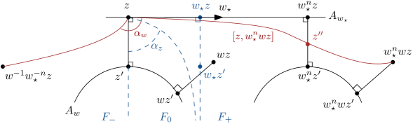
Figure 3. Proof of Lemma 4.7.

To see that (1) holds, first note that the segment $[z,w_{\star}^{n}wz]$ intersects $[w_{\star}^{n}z,w_{\star}^{n}z^{\prime}]$, because $w\uparrow w_{\star}$, and denote by $z^{\prime\prime}$ the intersection point. Then, as $[w_{\star}^{n}z,w_{\star}^{n}z^{\prime}]$ is orthogonal to $A_{w_{\star}}$, we have $\ell([z,z^{\prime\prime}])\geqslant n\ell([w_{\star}]).$ Moreover, as both $[w_{\star}^{n}z,w_{\star}^{n}z^{\prime}]$ and $[w_{\star}^{n}wz^{\prime},w_{\star}^{n}wz]$ are orthogonal to $w_{\star}^{n}A_{w}$, we have $\mathrm{dist}(z^{\prime\prime},w_{\star}^{n}wz)\geqslant\ell([w])$.

We prove (2) as follows. We have a decomposition in connected sets

$$\tilde{\Sigma}\setminus\bigl{(}(z,z^{\prime})\cup(w_{\star}z,w_{\star}z^{\prime})\bigr{)}=F_{-}\cup F_{0}\cup F_{+},$$

where $w_{\star,\pm}\in\overline{F_{\pm}}.$ Then since $w\uparrow w_{\star}$, we have $w_{\star}^{n}wz\in F_{+}$ for any $n\geqslant 1$ (since $wz\in F_{0}\cup F_{+}$) and thus the angle $\alpha_{w}$ between $[z^{\prime},z]$ and $[z,w_{\star}^{n}wz]$ is greater than the angle $\alpha_{z}$ between $(z,z^{\prime})$ and the ray joining $z$ to $(w_{\star}z,w_{\star}z^{\prime})_{+}$. Now $\alpha_{z}$ only depends on $z$ (and not on $w$), and we set $c=\inf_{y\in A_{w_{\star}}}\alpha_{y}>0$ (indeed $y\mapsto\alpha_{y}$ is continuous and $\alpha_{y}=\alpha_{w_{\star}y}$ for any $y\in A_{w_{\star}}$). As $w^{-1}w_{\star}^{-n}z\in F_{-}$, we get (2).

Now it is a classical fact from the theory of CAT($-\kappa$) spaces ($\kappa>0$) that the following holds. For $c>0$ as above, there is $C>0$ such that if $\eta\in\pi_{1}(\Sigma)\setminus\{1\}$ and $z\in\tilde{\Sigma}$ satisfy that the angle (taken in $[0,\pi]$) between $[\eta^{-1}z,z]$ and $[z,\eta z]$ is greater or equal than $c$, then $\ell(\eta)\geqslant\mathrm{dist}(z,\eta z)-C$ (see for example [PPS12, Lemma 2.8]). Applying this to $\eta=w_{\star}^{n}w$, we get with (1) and (2)

$$\ell([w_{\star}^{n}w])\geqslant\mathrm{dist}(z,w_{\star}^{n}wz)-C\geqslant n\ell([w_{\star}])+\ell([w])-C,\quad n\geqslant 1.$$ (4.9)

Here $C$ does not depend on $w$ such that $w\uparrow w_{\star}$. Now note that for $n>0$ one has

$$w\uparrow w_{\star}\quad\implies\quad w_{\star}^{n}w\uparrow w_{\star}.$$ (4.10)

Moreover, for $n>0$ large enough (depending on $w$), we have

$$w_{\star}^{\pm n}w\uparrow w_{\star}^{\pm 1}.$$

Therefore, if $n_{w}=\inf\{n\in\mathbb{Z},\leavevmode\nobreak\ w_{\star}^{n}w\uparrow w_{\star}\}$ we have, for any $n\geqslant 0$,

$$w_{\star}^{n}w_{\star}^{n_{w}}w\uparrow w_{\star}\quad\text{ and }\quad w_{\star}^{-n}w_{\star}^{n_{w}-1}~w\uparrow w_{\star}^{-1}.$$

Applying (4.9) with $w$ replaced by $w_{\star}^{n_{w}}w$ we get

$$\ell([w_{\star}^{n}w_{\star}^{n_{w}}w])\geqslant\ell([w_{\star}^{n_{w}}w])+n\ell([w_{\star}])-C,\quad n\geqslant 1.$$

Now applying (4.9) with $w_{\star}$ replaced by $w_{\star}^{-1}$ and $w$ replaced by $w_{\star}^{n_{w}-1}w$, we get

$$\ell([(w_{\star}^{-1})^{n}w_{\star}^{n_{w}-1}w])\geqslant\ell([w_{\star}^{n_{w}-1}w])+n\ell([w_{\star}])-C^{\prime},\quad n\geqslant 1.$$

The Lemma easily follows from the last two estimates, up to changing $C$ and $C^{\prime}$ and replacing $n_{w}$ by $n_{w}-1$. ∎

Proof of Proposition 4.3.

Let $j\in\{1,2\}$. For any primitive geodesic $\gamma_{j}\in\mathcal{P}(\Sigma_{j})$, we choose some $w_{\gamma_{j}}\in\pi_{1}(\Sigma_{j})$ such that $\gamma_{j}$ corresponds to the conjugacy class $[w_{\gamma_{j}}]$. We may assume that $\mathrm{wl}(w_{\gamma_{j}})=\mathrm{wl}([w_{\gamma_{j}}])$ where

$$\mathrm{wl}([w_{\gamma_{j}}])=\inf\left\{\mathrm{wl}(w^{\prime}_{j}),\leavevmode\nobreak\ w_{j}^{\prime}\in[w_{\gamma_{j}}]\right\}.$$

As $\pi_{1}(\Sigma_{j})$ is free, the element $w_{\gamma_{j}}$ is unique up to cyclic permutations. We denote $n_{j}(\gamma_{j})=\mathrm{wl}([w_{\gamma_{j}}])$ ; then the Milnor-Švarc lemma implies, for any $\gamma_{j}\in\mathcal{P}(\Sigma_{j})$ and $w_{j}\in[w_{\gamma_{j}}],$

$$\ell(\gamma_{j})=\ell([w_{\gamma_{j}}])=\ell([w_{j}])\leqslant\ell_{\star}(w_{j})\leqslant D\mathrm{wl}(w_{j})+D,$$

which gives

$$\ell(\gamma_{j})\leqslant Dn_{j}(\gamma_{j})+D,\quad\gamma_{j}\in\mathcal{P}(\Sigma_{j}).$$ (4.11)

Our goal is now the following. Starting from geodesics $\gamma_{j}\in\mathcal{P}(\Sigma_{j})$, $j=1,2$, we want to construct about $\ell(\gamma_{1})\ell(\gamma_{2})$ distinct geodesics in $\mathcal{P}$, by considering the conjugacy classes $[\bar{w}_{\gamma_{2}}\bar{w}_{\gamma_{1}}]$ where $\bar{w}_{\gamma_{j}}$ runs over all cyclic permutation of $w_{\gamma_{j}}$. However, as explained before, this process may conduct to produce several times the same geodesic in $\mathcal{P}$ (recall Lemma 4.6) so we are led to show estimates on the growth number of families of geodesics, as follows. For any $\gamma_{j}\in\mathcal{P}(\Sigma_{j})$, we define the family of conjugacy classes

$$\mathcal{C}_{\gamma_{j}}=\{[w_{\star,j}^{n}w_{\gamma_{j}}],\leavevmode\nobreak\ [w_{\star,j}^{n}w_{\gamma_{j}}]\text{ is primitive},\leavevmode\nobreak\ n\in\mathbb{Z}\}.$$

Here a class $[w]$ is said to be primitive if the closed geodesic corresponding to $[w]$ is primitive. We denote by $\mathscr{C}_{j}$ the set of such families, and for each $\mathcal{C}_{j}\in\mathscr{C}_{j}$ we set

$$\ell(\mathcal{C}_{j})=\min_{c\in\mathcal{C}_{j}}\ell(c).$$

The minimum exists by Lemma 4.7. We have the following

Lemma 4.8.

There is $C>0$ such that for $L$ big enough,

$$\#\{\mathcal{C}_{j}\in\mathscr{C}_{j},\leavevmode\nobreak\ \ell(\mathcal{C}_{j})\leqslant L\}~\geqslant C\mathrm{e}^{h_{\star}L}/L.$$

Proof.

By Lemma 4.7 we have for any $\gamma_{j}\in\mathcal{P}(\Sigma_{j})$

$$\#\{n\in\mathbb{Z},\leavevmode\nobreak\ \ell([w_{\star,j}^{n}w_{\gamma_{j}}])\leqslant L\}\leqslant C(L-\ell(\mathcal{C}_{\gamma_{j}})+C).$$

It follows that for large $L$,

$$N_{j}(L)=\sum_{\begin{subarray}{c}\gamma_{j}\in\mathcal{P}(\Sigma_{j})\\ \ell(\gamma_{j})\leqslant L\end{subarray}}1=\sum_{\begin{subarray}{c}\mathcal{C}_{j}\in\mathscr{C}_{j}\\ ~\ell(\mathcal{C}_{j})\leqslant L\end{subarray}}\#\{c\in\mathcal{C}_{j},\leavevmode\nobreak\ \ell(c)\leqslant L\}\leqslant C\sum_{\begin{subarray}{c}\mathcal{C}_{j}\in\mathscr{C}_{j}\\ ~\ell(\mathcal{C}_{j})\leqslant L\end{subarray}}(L-\ell(\mathcal{C}_{j})+C).$$

Let $\tilde{N}_{j}(L)=\#\{\mathcal{C}_{j}\in\mathscr{C}_{j},\leavevmode\nobreak\ \ell(\mathcal{C}_{j})\leqslant L\}.$ Then an Abel transformation gives

$$\sum_{\begin{subarray}{c}\mathcal{C}_{j}\in\mathscr{C}_{j}\\ ~\ell(\mathcal{C}_{j})\leqslant L\end{subarray}}(L-\ell(\mathcal{C}_{j})+C) \leqslant\sum_{k=1}^{L}\left(\tilde{N}_{j}(k)-\tilde{N}_{j}(k-1)\right)(L-k+C) \leqslant C^{\prime}\sum_{k=1}^{L}\tilde{N}_{j}(k),$$

and thus $\sum_{k=1}^{L}\tilde{N}_{j}(k)\geqslant C\exp({h_{\star}L})/L$ for large $L$. On the other hand we have for $M>0$

$$\sum_{k=1}^{L-M}\tilde{N}_{j}(k)\leqslant\sum_{k=1}^{L-M}N_{j}(k)\leqslant C\sum_{k=1}^{L-M}\frac{\mathrm{e}^{h_{\star}k}}{k}\leqslant C^{\prime}\frac{\mathrm{e}^{h_{\star}(L-M)}}{L-M}.$$

Therefore, if $M$ is big enough, we have for any $L$ large enough

$$M\tilde{N}_{j}(L)\geqslant\sum_{k=L-M}^{L}\tilde{N}_{j}(k)\geqslant\frac{N_{j}(L)}{2}\geqslant C^{\prime\prime}\mathrm{e}^{h_{\star}L}/L,$$

which concludes. ∎

For any $\mathcal{C}_{j}\in\mathscr{C}_{j}$, we choose some class $[w_{\mathcal{C}_{j}}]\in\mathcal{C}_{j}$ such that $\ell(\mathcal{C}_{j})=\ell([w_{\mathcal{C}_{j}}])$. Also $w_{\mathcal{C}_{j}}\in\pi_{1}(\Sigma_{j})$ may be chosen cyclically reduced, meaning that $\mathrm{wl}(w_{\mathcal{C}_{j}})=\mathrm{wl}([w_{\mathcal{C}_{j}}])$. Let $W_{\mathcal{C}_{j}}\subset\pi_{1}(\Sigma_{j})$ denote the set of cyclic permutations of $w_{\mathcal{C}_{j}}$ Then $|W_{\mathcal{C}_{j}}|=\mathrm{wl}([w_{\mathcal{C}_{j}}])$ since $w_{\mathcal{C}_{j}}$ is primitive (see [LS62]).

Lemma 4.9.

For any $\mathcal{C}_{j}\in\mathscr{C}_{j}$, there exists a subset $W_{\mathcal{C}_{j}}^{\prime}\subset W_{\mathcal{C}_{j}}$ with

$$|W_{\mathcal{C}_{j}}^{\prime}|\geqslant(|W_{\mathcal{C}_{j}}|-3)/4$$

and the following property. For any $p,q\in\mathbb{Z}$ and $w\in W_{\mathcal{C}_{j}}^{\prime}$,

$$(w_{\star,j})^{p}w(w_{\star,j})^{q}\in W_{\mathcal{C}_{j}}^{\prime}\quad\implies\quad p=q=0.$$

Proof.

We prove the lemma for $j=1$. Let $\mathcal{C}_{1}\in\mathscr{C}_{1}$ ; we set $\mathrm{g}=\mathrm{g}_{1},w_{\star}=w_{\star,1}$ and $W=W_{\mathcal{C}_{1}}$ to simplify notations. For $w\in W$, we will say that $w$ is of type $A$ if $(w_{\star})^{p}w(w_{\star})^{q}\in W_{\mathcal{C}_{1}}$ for some $p,q\in\mathbb{Z}\setminus(0,0)$. If $w$ is of type $A$, then exactly $2\mathrm{g}(|p|+|q|)\geqslant 2$ simplifications occur in the word $w^{\prime}=(w_{\star})^{p}w(w_{\star})^{q}$, since $\mathrm{wl}(w_{\star})=4\mathrm{g}$. As $w_{\star}=a_{1}b_{1}a_{1}^{-1}b_{1}^{-1}\cdots a_{\mathrm{g}}^{-1}b_{\mathrm{g}}^{-1}$ and at least $2$ simplifications occur in $w$’, we see that $w$ has necessarily one of the following forms :

$$a_{1}b_{1}\cdots a_{1}\cdots b_{\mathrm{g}}^{-1} \cdots b_{1}^{-1}a_{1}^{-1}$$ (1) (3) (5)

$$b_{\mathrm{g}}a_{\mathrm{g}}\cdots b_{\mathrm{g}}\cdots a_{1}^{-1} \cdots a_{\mathrm{g}}^{-1}b_{\mathrm{g}}^{-1}$$ (2) (4) (6)

Denote $n=\mathrm{wl}(w)$ and $w=u_{1}\cdots u_{n}$ with $u_{j}\in\{a_{k},b_{k},a_{k}^{-1},b_{k}^{-1},\leavevmode\nobreak\ k=1,\dots,\mathrm{g}\}$. Set $w_{k}=u_{\sigma^{k}(1)}\cdots u_{\sigma^{k}(n)}$ for $k\in\mathbb{N}$ where $\sigma$ is the permutation sending $(1,\dots,n)$ to $(n,1,\dots,n-1)$, so that $W=\{w_{k},\leavevmode\nobreak\ k=1,\dots,n\}.$

Assume that $w_{k}$ is of type $A$. If $w_{k}$ is of the form (5) or (6), it is clear that $w_{k+1}$ cannot be of type $A$. If $w_{k}$ is of the form (3) or (4), and if $w_{k+1}$ is of type $A$, $w_{k+1}$ is necessarily the form (5) or (6), so that $w_{k+2}$ cannot be of type $A$. Finally assume that $w_{k}$ is of the form (1) or (2). Then we see that $w_{k+1}$ cannot be of the form (1) or (2) except if $\mathrm{g}=1$. Therefore if $w_{k+1}$ is still of type $A$ and $\mathrm{g}>1$, it has one of the forms (3), (4), (5) or (6) and $w_{k+2}$ or $w_{k+3}$ is not of type $A$ by what precedes. We showed that if $\mathrm{g}>1$ and $w_{k}$ is of type $A$, one of the words $w_{k+1},w_{k+2},w_{k+3}$ is not of type $A$. Therefore by denoting $W^{\prime}$ the set of words which are not of type $A$, the conclusion of the lemma holds.

Now suppose $\mathrm{g}=1$ so that $w_{\star}=a_{1}b_{1}a_{1}^{-1}b_{1}^{-1}$. If $w_{k}$ is of type $A$ and not of the form (1) or (2), then $w_{k+1}$ or $w_{k+2}$ is not of type $A$ by what precedes. Thus we assume that $w_{k}$ is of the form (1) or (2), but not of the form (3), (4), (5) or (6) (such words will be called of type $B$). In particular, we have $w_{k}=\cdots u_{\sigma^{k}(n)}$ with $u_{\sigma^{k}(n)}\neq b_{1}^{-1},a_{1}^{-1}$ (as $\mathrm{g}=1$). Thus, in the word $(w_{\star})^{p}w_{k}(w_{\star})^{q}$, simplifications can only occur between $(w_{\star})^{p}$ and $w$, and it is not hard to see that $\#(\mathcal{O}_{k})\leqslant 2$ where

$$\mathcal{O}_{k}=\{(w_{\star})^{p}w_{k}(w_{\star})^{q},\leavevmode\nobreak\ p,q\in\mathbb{Z}\}\cap W.$$

Denote $\mathscr{O}=\{\mathcal{O}_{k},\leavevmode\nobreak\ k=1,\dots,n,\leavevmode\nobreak\ w_{k}\text{ is of type }B\}.$ For any $\mathcal{O}\in\mathscr{O}$ we choose some $w_{\mathcal{O}}\in\mathcal{O}$. Then

$$W^{\prime}=\{w\in W,\leavevmode\nobreak\ w\text{ is not of type }A\}~\cup\{w_{\mathcal{O}},\leavevmode\nobreak\ \mathcal{O}\in\mathscr{O}\}$$

satisfies the conclusion of the lemma. ∎

Using Lemmas 4.5 and 4.6 we thus obtain that the map

$$\begin{matrix}\displaystyle{\bigcup_{(\mathcal{C}_{1},\mathcal{C}_{2})\in\mathscr{C}_{1}\times\mathscr{C}_{2}}}&W_{\mathcal{C}_{1}}^{\prime}\times W_{\mathcal{C}_{2}}^{\prime}&\longrightarrow&\mathcal{P},\\ &(w_{1},w_{2})&\longmapsto&[w_{2}w_{1}]\end{matrix}$$

is injective. Moreover for any $(w_{1},w_{2})$ we have $\ell([w_{2}w_{1}])\leqslant\ell([w_{1}])+\ell([w_{2}])+4\operatorname{diam}\Sigma+2$. Indeed, let $\gamma_{j}\in\mathcal{P}(\Sigma_{j})$ denote the unique geodesic corresponding to the class $[w_{j}]$ for $j=1,2$. Then we may find a smooth curve $\tilde{\gamma}_{j}$ based at $x_{\star}$ such that $\tilde{\gamma}_{j}=w_{j}$ as elements of $\pi_{1}(\Sigma_{j})$ and $\ell(\tilde{\gamma}_{j})\leqslant\ell([w_{j}])+2\operatorname{diam}\Sigma+1$ (for example by removing some appropriate small piece of $\gamma_{j}$ and link the endpoints of the cutted curve to $x_{\star}$). Thus $\ell([w_{2}w_{1}])\leqslant\ell(\tilde{\gamma}_{2}\tilde{\gamma}_{1})\leqslant\ell(\gamma_{1})+\ell(\gamma_{2})+4\operatorname{diam}\Sigma+2=\ell([w_{1}])+\ell([w_{2}])+4\operatorname{diam}\Sigma+2.$ We thus obtain, with $R=4\operatorname{diam}\Sigma+2$ and $C$ being a constant changing at each line,

$$\sum_{\begin{subarray}{c}\gamma\in\mathcal{P}\\ i(\gamma,\gamma_{\star})=2\\ ~\ell(\gamma)\leqslant L\end{subarray}}1 \geqslant\sum_{\begin{subarray}{c}(\mathcal{C}_{1},\mathcal{C}_{2})\\ \ell(\mathcal{C}_{1})+\ell(\mathcal{C}_{2})\leqslant L-R\end{subarray}}|W_{\mathcal{C}_{1}}^{\prime}|~|W_{\mathcal{C}_{2}}^{\prime}|$$

$$\geqslant\sum_{\begin{subarray}{c}(\mathcal{C}_{1},\mathcal{C}_{2})\\ \ell(\mathcal{C}_{1})+\ell(\mathcal{C}_{2})\leqslant L-R\end{subarray}}\left(C\ell(\mathcal{C}_{1})-C\right)\left(C\ell(\mathcal{C}_{2})-C\right)$$

$$=A(L)+C\sum_{\begin{subarray}{c}(\mathcal{C}_{1},\mathcal{C}_{2})\\ \ell(\mathcal{C}_{1})+\ell(\mathcal{C}_{2})\leqslant L-R\end{subarray}}\ell(\mathcal{C}_{1})\ell(\mathcal{C}_{2})$$

where we used $|W_{\mathcal{C}_{j}}^{\prime}|\geqslant C|W_{\mathcal{C}_{j}}|-C=C\mathrm{wl}(w_{j})-C\geqslant\displaystyle{C\ell(\mathcal{C}_{j})-C}$ for $j=1,2$ (this follows by Lemma 4.9 and (4.11)) and the fact that $\ell(w_{j})=\ell(\mathcal{C}_{j})$ for any $w_{j}\in W_{j}$, and where

$$A(L)\leqslant C\sum_{\begin{subarray}{c}(\mathcal{C}_{1},\mathcal{C}_{2})\\ \ell(\mathcal{C}_{1})+\ell(\mathcal{C}_{2})\leqslant L-R\end{subarray}}(\ell(\mathcal{C}_{1})+\ell(\mathcal{C}_{2})+1).$$

By Lemma 4.8 we have

$$C^{-1}\mathrm{e}^{h_{\star}L}/L\leqslant\#\{\mathcal{C}_{j},\leavevmode\nobreak\ ~\ell(\mathcal{C}_{j})\leqslant L\}\leqslant C\mathrm{e}^{h_{\star}L}/L,$$ (4.12)

and from this it is not hard to see that $A(L)\ll L\mathrm{e}^{h_{\star}L}$ as $L\to+\infty.$ Moreover, using (4.12) and similar techniques we used to obtain (4.7) (for example by noting that there is $C$ such that $\tilde{N}_{j}(L)-\tilde{N}_{j}(L-C)\geqslant C\mathrm{e}^{h_{\star}L}/L$ for any $L$ large enough, where $\tilde{N}_{j}(L)=\#\{\mathcal{C}_{j},\leavevmode\nobreak\ ~\ell(\mathcal{C}_{j})\leqslant L\}$, as it follows from (4.12)) we get for $L$ large enough

$$\sum_{\begin{subarray}{c}(\mathcal{C}_{1},\mathcal{C}_{2})\\ \ell(\mathcal{C}_{1})+\ell(\mathcal{C}_{2})\leqslant L-R\end{subarray}}\ell(\mathcal{C}_{1})\ell(\mathcal{C}_{2})\geqslant C(L-R)\mathrm{e}^{h(L-R)},$$

which concludes the proof of Proposition 4.3. ∎

4.2.2. Upper bound

Each $\gamma\in\mathcal{P}_{2}$ with $\ell(\gamma)\leqslant L$ is in the conjugacy class $w_{1}w_{2}$ for some $w_{j}\in\pi_{1}(\Sigma_{j})$ with $\ell_{\star}(w_{1})+\ell_{\star}(w_{2})\leqslant L+C$. Therefore (4.2) implies

$$N(2,L) \leqslant\sum_{\begin{subarray}{c}w_{j}\in\pi_{1}(\Sigma_{j})\\ ~\ell_{\star}(w_{1})+\ell_{\star}(w_{2})\leqslant L+C\end{subarray}}1$$

$$\leqslant\sum_{k=0}^{L+C}C\exp(h_{1}k)\exp(h_{2}(L-k+C)),$$

which gives for large $L$, if $h_{\star}=\max(h_{1},h_{2})$,

$$N(2,L)\leqslant\left\{~\begin{matrix}CL\exp(h_{\star}L)&\text{ if }&h_{1}=h_{2},\vspace{0.15cm}\\ C\exp(h_{\star}L)&\text{ if }&h_{1}\neq h_{2}.\end{matrix}~\right.$$

Iterating this process we obtain (with $C$ depending on $n$)

$$N(n,L)\leqslant\left\{~\begin{matrix}CL^{2n-1}\exp(h_{\star}L)&\text{ if }&h_{1}=h_{2},\vspace{0.15cm}\\ CL^{n-1}\exp(h_{\star}L)&\text{ if }&h_{1}\neq h_{2}.\end{matrix}~\right.$$

4.3. Relative growth of geodesics with small intersection angle

For any $\eta>0$ small, we consider $N(n,\eta,L)=\#(\mathcal{P}_{\eta,n}(L))$ where $\mathcal{P}_{\eta,n}(L)$ is the set of closed geodesics $\gamma:\mathbb{R}/\mathbb{Z}\to\Sigma$ of length not greater than $L$, intersecting $\gamma_{\star}$ exactly $n$ times, and such that there is $\tau$ with $\gamma(\tau)\in\gamma_{\star}$ and $\mathrm{angle}(\dot{\gamma}(\tau),T_{\gamma(\tau)}\gamma_{\star})<\eta.$ The purpose of this paragraph is to prove the following estimate.

Lemma 4.10.

For any $L_{0}>0$, there is $\eta>0$ such that for any $L$ big enough

$$N(n,\eta,L)\leqslant 2nN(n,L-L_{0}).$$

Proof.

Let $P_{2n}(\mathcal{P}_{n})$ denote the set of subsets of $\mathcal{P}_{n}$ which are of cardinal not greater than $2n$. Then for $K\in\mathbb{N}_{\geqslant 1}$ we construct a map

$$\Psi_{K}:\mathcal{P}_{n}\to P_{2n}(\mathcal{P}_{n}),$$

as follows. Let $\gamma:\mathbb{R}/\mathbb{Z}\to\Sigma$ be an element of $\mathcal{P}_{n}$ and let $\tau_{1},\dots,\tau_{n}\in\mathbb{R}/\mathbb{Z}$ be pairwise distinct such that $\gamma(\tau_{j})\in\gamma_{\star}$. For any $j$, choose a path $c_{j}$ contained in $\gamma_{\star}$ and linking $x_{\star}$ to $\gamma(\tau_{j}).$ Then set $w_{j}=c_{j}^{-1}\gamma_{j}c_{j}\in\pi_{1}(\Sigma)$, where $\gamma_{j}:\mathbb{R}/\mathbb{Z}\to\Sigma$ is defined by $\gamma_{j}(t)=\gamma(\tau_{j}+t).$ Then set

$$\Psi_{K}(\gamma)=\left\{\left[w_{j}w_{\star}^{\varepsilon K}\right],\leavevmode\nobreak\ j=1,\dots,n,\leavevmode\nobreak\ ~\varepsilon\in\{-1,1\}\right\}\in P_{2n}(\mathcal{P}_{n}).$$

Here the class $\left[w_{j}w_{\star}^{\varepsilon K}\right]$ is identified with the unique geodesic contained in the free homotopy class of $w_{j}w_{\star}^{\varepsilon K}$. Note that $\Psi_{K}$ is well defined: for different choices of $c_{j}$, we would obtain $w_{\star}^{k_{j}}w_{j}w_{\star}^{-k_{j}}$ instead of $w_{j}$ for some $k_{j}\in\mathbb{Z}$; however the class $\left[w_{\star}^{k_{j}}w_{j}w_{\star}^{-k_{j}}w_{\star}^{\varepsilon K}\right]$ coincides with $\left[w_{j}w_{\star}^{\varepsilon K}\right]$. Moreover, the image of $\Psi_{K}$ is indeed contained in $\mathcal{P}_{n}$. Indeed, by similar techniques used to prove Lemma 4.5, one can show that the geodesic $[w_{j}w_{\star}^{\varepsilon K}]$ intersects $\gamma_{\star}$ exactly $n$ times, as $\gamma$ does (adding turns aroung $\gamma_{\star}$ does not change the intersection number with $\gamma_{\star}$).

Our goal is now to show that there is $C>0$ such that for any $K\in\mathbb{N}_{\geqslant 1}$, there is $\eta>0$ such that

$$\mathcal{P}_{\eta,n}(L)\subset\bigcup_{\gamma\in\mathcal{P}_{n}(L-K\ell(\gamma_{\star})+C)}\Psi_{K}(\gamma).$$ (4.13)

Let $\varepsilon>0$ smaller than $\rho_{g}/2$ where $\rho_{g}$ is the injectivity radius of $(\Sigma,g)$, and $K\in\mathbb{N}_{\geqslant 1}$. Then there is $\eta>0$ such that if $z=(0,\tau,\theta)\in\gamma_{\star}$ (here we use the coordinates of Lemma 2.2) with $|\theta|<\eta$ (resp. $|\theta-\pi|~<\eta$), then if $z^{\prime}=(0,\tau,0)$ (resp. $z^{\prime}=(0,\tau,\pi)$), we have

$$\mathrm{dist}_{\Sigma}(\pi(\varphi_{t}(z)),\pi(\varphi_{t}(z^{\prime})))\leqslant\varepsilon,\quad t\in[0,K\ell(\gamma_{\star})].$$

Let $c(t)=\pi(\varphi_{t}(z))$ for $t\in[0,K\ell(\gamma_{\star})]$, and close the path $c$ by using the exponential map at $\pi(z)$, to obtain a closed curve $\tilde{\gamma}:\mathbb{R}/\mathbb{Z}\to\Sigma$ of length not greater than $K\ell(\gamma_{\star})+2\varepsilon$. If $\varepsilon$ (and thus $\eta$) is small enough, we have $\tilde{\gamma}=\gamma_{\star}^{\pm K}$ in $\pi_{1}(\Sigma,\pi(z))$ whenever $|\sin\theta|<\eta$. In particular, if $\gamma:\mathbb{R}/\ell(\gamma)\mathbb{Z}\to\Sigma$ is a closed geodesic intersecting $\gamma_{\star}$ exactly $n$ times, and with at least one intersection angle smaller than $\eta$, then we can write

$$\gamma\sim w_{\star}^{\pm K}w^{\prime}$$ (4.14)

for some $w^{\prime}\in\pi_{1}(\Sigma)$, satisfying $\ell_{\star}(w^{\prime})\leqslant\ell(\gamma)-K\ell(\gamma_{\star})+C$ (for some $C>0$ independent of $\gamma$). Here $a\sim b$ means that $a$ is freely homotopic to $b$. As before, the unique geodesic contained in the free homotopy class of $w^{\prime}$ intersects $\gamma_{\star}$ exactly $n$ times (removing some turns around $\gamma_{\star}$ does not change the intersection number).

Finally, by similar techniques used in the proofs of Lemmas 4.2 or 4.6, one can see that $[w^{\prime}w_{\star}^{\pm K}]\in\Psi_{K}([w^{\prime}])$ (again, we identify the geodesic freely homotopic to $w^{\prime}$ with the class $[w^{\prime}]$) for any $w^{\prime}\in\pi_{1}(\Sigma)$ such that $i([w^{\prime}],\gamma_{\star})=n$. Moreover, if $\ell_{\star}(w^{\prime})\leqslant\ell(\gamma)-K\ell(\gamma_{\star})+C$, then we have of course $\ell([w^{\prime}])\leqslant\ell_{\star}(w^{\prime})\leqslant\ell(\gamma)-K\ell(\gamma_{\star})+C$. Thus (4.14) implies that each $\gamma\in\mathcal{P}_{\eta,n}(L)$ lies in $\Psi(\gamma^{\prime})$ for some $\gamma^{\prime}\in\mathcal{P}_{n}$ (given by $[w^{\prime}]$) such that $\ell(\gamma^{\prime})\leqslant L-K\ell(\gamma_{\star})+C$. The lemma follows. ∎

5. A Tauberian argument

The goal of this section is to give an asymptotic growth of the quantity

$$N_{\pm}(n,\chi,t)=\sum_{\begin{subarray}{c}\gamma\in\mathcal{P}\\ ~i(\gamma_{\star},\gamma)=n\\ \ell(\gamma)\leqslant t\end{subarray}}I_{\star,\pm}(\gamma,\chi)$$

as $t\to+\infty$, where $\chi\in C^{\infty}_{c}(\partial\setminus\partial_{0})$ and $I_{\star,\pm}(\gamma,\chi)=\prod_{z\in I_{\star,\pm}(\gamma)}\chi(z).$

5.1. The case $\gamma_{\star}$ is not separating

By [DG16], we know that the zeta function

$$\zeta_{\Sigma_{\star}}(s)=\prod_{\gamma\in\mathcal{P}_{\star}}\left(1-\mathrm{e}^{-s\ell(\gamma)}\right)$$

extends meromorphically to the whole complex plane, and moreover we may write

$$\zeta_{\Sigma_{\star}}^{\prime}(s)/\zeta_{\Sigma_{\star}}(s)=\sum_{k=0}^{2}(-1)^{k}\mathrm{tr}^{\flat}\left(\mathrm{e}^{\pm\varepsilon s}\varphi_{\mp\varepsilon}^{*}R_{\pm,\delta}(s)|_{\Omega^{k}_{c}(M_{\delta})\cap\ker\iota_{X}}\right),$$

where the flat trace is computed on $M_{\delta}$. Here $\mathcal{P}_{\star}$ denote the set of primitive closed geodesics of $(\Sigma_{\star},g)$. By [PP90], $\zeta_{\Sigma_{\star}}^{\prime}/\zeta_{\Sigma_{\star}}$ is holomorphic in $\{\operatorname{Re}(s)\geqslant h\}$ except for a simple pole at $s=h_{\star}$, where $h_{\star}>0$ is the topological entropy of the geodesic flow of $(\Sigma_{\star},g)$ restricted to the trapped set (as defined in the introduction). Moreover, it is shown in [DG16] that $s\mapsto R_{\pm,\delta}(s)|_{\Omega^{k}\cap\ker\iota_{X}}$ has no pole in $\{\operatorname{Re}(s)>0\}$ for $k=0$ and $k=2$. Write the Laurent expansion of $R_{\pm,\delta}(s)$ given in §2.5 near $s=h_{\star}$ as

$$R_{\pm,\delta}(s)=Y_{\pm,\delta}(s)+\frac{\Pi_{\pm,\delta}(h_{\star})}{s-h_{\star}}:\Omega^{\bullet}_{c}(M_{\delta})\to\mathcal{D}^{\prime\bullet}(M_{\delta}).$$

Denote $\Omega^{k}=\Omega^{k}_{c}(M_{\delta})$ and $\Omega^{k}_{0}=\Omega^{k}\cap\ker\iota_{X}.$ Then the above comments show that

$$\operatorname{rank}(\Pi_{\pm,\delta}|_{\Omega^{1}_{0}})=1.$$

As $R_{\pm,\delta}(s)$ commutes with $\iota_{X}$, it preserves the spaces $\Omega^{k}_{0}$. Writing $\Omega^{k}=\Omega^{k}_{0}\oplus\alpha\wedge\Omega^{k-1}_{0}$ we have for any $w=u+\alpha\wedge v$ with $\iota_{X}u=0$ and $\iota_{X}v=0$,

$$\Pi_{\pm,\delta}(h_{\star})|_{\Omega^{2}}(u+\alpha\wedge v)=\Pi_{\pm,\delta}(h_{\star})|_{\Omega^{2}_{0}}(u)+\alpha\wedge\Pi_{\pm,\delta}(h_{\star})|_{\Omega^{1}_{0}}(v).$$

Thus $\Pi_{\pm,\delta}|_{\Omega^{2}}=\alpha\wedge\iota_{X}\Pi_{\pm,\delta}|_{\Omega^{1}_{0}}$. By Proposition 3.2 and the fact that $\varphi_{\pm\varepsilon}^{*}\Pi_{\pm,\delta}(h_{\star})=\mathrm{e}^{\pm\varepsilon h_{\star}}\Pi_{\pm,\delta}(h_{\star}),$ we have near $s=h_{\star}$

$$\tilde{\mathcal{S}}_{\pm}(s)=Y_{\pm}(s)+\frac{\psi^{*}\iota^{*}\iota_{X}\Pi_{\pm,\delta}(h_{\star})\iota_{*}}{s-h_{\star}},$$

where $Y_{\pm}(s)$ is holomorphic near $s=h_{\star}$. We denote

$$\Pi_{\pm,\partial}=\psi^{*}\iota^{*}\iota_{X}\Pi_{\pm,\delta}(h_{\star})\iota_{*}:\Omega^{\bullet}(\partial)\to\mathcal{D}^{\prime\bullet}(\partial).$$

Then by what precedes, and since $\iota_{X}\Pi_{\pm,\delta}(h_{\star})|_{\Omega^{1}}=0$, we obtain that $\operatorname{rank}(\Pi_{\pm,\partial})=1$. Finally for any $\chi\in C^{\infty}_{c}(\partial\setminus\partial_{0})$ we set

$$c_{\pm}(\chi)={\operatorname{tr}}_{\mathrm{s}}^{\flat}(\chi\Pi_{\pm,\partial}).$$

Lemma 5.1.

Let $\chi\in C^{\infty}_{c}(\partial\setminus\partial_{0})$ such that $c_{\pm}(\chi)>0$. Then it holds

$$N_{\pm}(n,\chi,t)\sim\frac{(c_{\pm}(\chi)t)^{n}}{n!}~\frac{\mathrm{e}^{h_{\star}t}}{h_{\star}t},\quad t\to+\infty.$$

Proof.

Because $\chi\Pi_{\pm,\partial}$ is of rank one, it follows that ${\operatorname{tr}}_{\mathrm{s}}^{\flat}((\chi\Pi_{\pm,\partial})^{n})=c_{\pm}(\chi)^{n}$ for any $n\geqslant 1$ (since the flat trace of finite rank operator coincide with its usual trace) and thus

$${\operatorname{tr}}_{\mathrm{s}}^{\flat}((\chi\tilde{\mathcal{S}}_{\pm}(s))^{n})=\frac{c_{\pm}(\chi)^{n}}{(s-h_{\star})^{n}}+\mathcal{O}((s-h_{\star})^{-n+1}),\quad s\to h_{\star}.$$

We set $\eta_{n,\chi}(s)={\operatorname{tr}}_{\mathrm{s}}^{\flat}((\chi\tilde{\mathcal{S}}_{\pm}(s))^{n}),$ and

$$g_{n,\chi}(t)=\sum_{\begin{subarray}{c}\gamma\in\mathcal{P}\\ i(\gamma,\gamma_{\star})=n\end{subarray}}\ell(\gamma)\sum_{\begin{subarray}{c}k\geqslant 1\\ ~k\ell(\gamma)\leqslant t\end{subarray}}I_{\star,\pm}(\gamma,\chi)^{k},\quad t\geqslant 0,$$

Now if $G_{n,\chi}(s)=\displaystyle{\int_{0}}^{+\infty}g_{n,\chi}(t)\mathrm{e}^{-ts}\mathrm{d}t$, a simple computation leads to

$$G_{n,\chi}(s)=\frac{1}{s}\sum_{i(\gamma,\gamma_{\star})=n}\ell^{\#}(\gamma)\mathrm{e}^{-s\ell(\gamma)}I_{\star,\pm}(\gamma,\chi)^{\ell(\gamma)/\ell^{\#}(\gamma)}=-\frac{\eta_{n,\chi}^{\prime}(s)}{ns},$$

where the last equality comes from Proposition 3.6. Because one has the expansion $\eta_{n,\chi}^{\prime}(s)=-nc_{\pm}(\chi)^{n}(s-h_{\star})^{-(n+1)}+\mathcal{O}((s-h_{\star})^{-n})$ as $s\to h_{\star}$, we obtain

$$G_{n,\chi}(h_{\star}s)=\frac{c_{\pm}(\chi)^{n}}{h_{\star}^{n+2}(s-1)^{n+1}}+\mathcal{O}((s-h_{\star})^{-n}),\quad s\to h_{\star}.$$

Then applying the Tauberian theorem of Delange [Del54, Théorème III], we have

$$\frac{1}{h_{\star}}g_{n,\chi}(t/h_{\star})\sim\frac{c_{\pm}(\chi)^{n}}{h_{\star}^{n+2}}\frac{\mathrm{e}^{t}}{n!}t^{n},\quad t\to+\infty,$$

which reads

$${g_{n,\chi}(t)\sim\frac{(c_{\pm}(\chi)t)^{n}}{n!h_{\star}}\exp(h_{\star}t).}$$ (5.1)

Now note that, if $\mathcal{P}_{n}$ is the set of primitive closed geodesics $\gamma$ with $i(\gamma,\gamma_{\star})=n$ one has

$$g_{n,\chi}(t)\leqslant\sum_{\begin{subarray}{c}\gamma\in\mathcal{P}_{n}\\ ~\ell(\gamma)\leqslant t\end{subarray}}\ell(\gamma)\lfloor t/\ell(\gamma)\rfloor I_{\gamma}(\chi)\leqslant tN(n,\chi,t).$$

As a consequence we have

$$\liminf_{t\to+\infty}N_{\pm}(n,\chi,t)\frac{n!h_{\star}t}{(c_{\pm}(\chi)t)^{n}\mathrm{e}^{h_{\star}t}}\geqslant 1.$$ (5.2)

For the other bound, we use the a priori bound obtained in §4.1.2

$$N_{\pm}(n,\chi,t)\leqslant N(n,t)\leqslant\frac{Ct^{n}}{n!}\frac{\mathrm{e}^{h_{\star}t}}{h_{\star}t}$$

to deduce that for any $\sigma>1$

$$\limsup_{t\to+\infty}N_{\pm}(n,\chi,t/\sigma)\frac{n!}{t^{n}}\frac{h_{\star}t}{\mathrm{e}^{h_{\star}t}}=0.$$ (5.3)

Now we may write

$$N_{\pm}(n,\chi,t) =N_{\pm}(n,\chi,t/\sigma)+\sum_{\begin{subarray}{c}\gamma\in\mathcal{P}\\ ~i(\gamma_{\star},\gamma)=n\\ t/\sigma\leqslant\ell(\gamma)\leqslant t\end{subarray}}I_{\star,\pm}(\gamma,\chi)$$

$$\leqslant N_{\pm}(n,\chi,t/\sigma)+\frac{\sigma}{t}\sum_{\begin{subarray}{c}\gamma\in\mathcal{P}\\ ~i(\gamma_{\star},\gamma)=n\\ t/\sigma\leqslant\ell(\gamma)\leqslant t\end{subarray}}I_{\star,\pm}(\gamma,\chi)\ell(\gamma)$$

$$\leqslant N_{\pm}(n,\chi,t/\sigma)+\frac{\sigma}{t}g_{n,\chi}(t),$$

which gives with (5.3)

$$\limsup_{t\to+\infty}N_{\pm}(n,\chi,t)\frac{n!}{(c_{\pm}(\chi)t)^{n}}\frac{h_{\star}t}{\mathrm{e}^{h_{\star}t}}\leqslant\sigma.$$

As $\sigma>1$ is arbritrary, the Lemma is proven. ∎

5.2. The case $\gamma_{\star}$ is separating

In that case, $\Sigma_{\delta}$ consists of two surfaces $\Sigma_{\delta}^{(1)}$ and $\Sigma_{\delta}^{(2)}$. We write $M_{\delta}=M_{\delta}^{(1)}\sqcup M_{\delta}^{(2)}$ where $M_{\delta}^{(j)}=S\Sigma_{\delta}^{(j)}$, $j=1,2,$ and $\partial=\partial^{(1)}\sqcup\partial^{(2)}$ with $\partial^{(j)}\subset M_{\delta}^{(j)}$. Note that, if $\tilde{\mathcal{S}}_{\pm}^{(j)}(s)$ denotes the restriction of $\tilde{\mathcal{S}}_{\pm}(s)$ to $\partial^{(j)},$ we have

$$\tilde{\mathcal{S}}_{\pm}^{(1)}(s):\Omega^{\bullet}(\partial^{(1)})\to\mathcal{D}^{\prime\bullet}(\partial^{(2)}),\quad\tilde{\mathcal{S}}_{\pm}^{(2)}(s):\Omega^{\bullet}(\partial^{(2)})\to\mathcal{D}^{\prime\bullet}(\partial^{(1)}).$$

As in §5.1, we have

$$\tilde{\mathcal{S}}_{\pm}^{(j)}(s)=Y_{\pm}^{(j)}(s)+\frac{\Pi_{\pm,\partial}^{(j)}}{s-h_{j}},\quad s\to h_{j},$$

where $Y_{\pm}^{(j)}(s)$ is holomorphic near $s=h_{j}$ and $h_{j}$ is the topological entropy of the geodesic flow of $\Sigma_{\delta}^{(j)}.$ As before we fix $\chi\in C^{\infty}_{c}(\partial\setminus\partial_{0})$.

5.2.1. The case $h_{1}\neq h_{2}$

We may assume $h_{1}>h_{2}$ and we set $c_{\pm}(\chi)={\operatorname{tr}}_{\mathrm{s}}^{\flat}\left(\chi\tilde{\mathcal{S}}_{\pm}^{(2)}(h_{1})\chi\Pi_{\pm,\partial}^{(1)}\right).$ Because $\Pi_{\pm,\partial}^{(1)}$ is of rank one, it follows that ${\operatorname{tr}}_{\mathrm{s}}^{\flat}\left(\bigl{(}\chi\tilde{\mathcal{S}}_{\pm}^{(2)}(h_{1})\chi\Pi_{\pm,\partial}^{(1)}\bigr{)}^{n}\right)=c_{\pm}(\chi)^{n}$ for any $n\geqslant 1$ and thus, by cyclicity of the flat trace (as the flat trace coincide with the real trace for operators of finite rank), we have as $s\to h_{1}$,

$${\operatorname{tr}}_{\mathrm{s}}^{\flat}\left((\chi\tilde{\mathcal{S}}_{\pm}(s))^{2n}\right) ={\operatorname{tr}}_{\mathrm{s}}^{\flat}\left(\bigl{(}\chi\tilde{\mathcal{S}}_{\pm}^{(1)}(s)\chi\tilde{\mathcal{S}}_{\pm}^{(2)}(s)\bigr{)}^{n}+\bigl{(}\chi\tilde{\mathcal{S}}_{\pm}^{(2)}(s)\chi\tilde{\mathcal{S}}_{\pm}^{(1)}(s)\bigr{)}^{n}\right)$$

$$=\frac{2c_{\pm}(\chi)^{n}}{(s-h_{1})^{n}}+\mathcal{O}((s-h_{1})^{-n+1}).$$

Now we may proceed exactly as in §5.1 to obtain that, if $c_{\pm}(\chi)>0$,

$$N(2n,\chi,t)\sim\frac{(c_{\pm}(\chi)t)^{n}}{n!}\frac{\mathrm{e}^{h_{\star}t}}{h_{\star}t},\quad t\to+\infty.$$

5.2.2. The case $h_{1}=h_{2}=h_{\star}$

In that case, by denoting $c_{\pm}(\chi)={\operatorname{tr}}_{\mathrm{s}}^{\flat}(\Pi_{\pm,\partial}^{(1)}\Pi_{\pm,\partial}^{(2)})$ we have

$${\operatorname{tr}}_{\mathrm{s}}^{\flat}\left((\chi\tilde{\mathcal{S}}_{\pm}(s))^{2n}\right)=\frac{2c_{\pm}(\chi)^{n}}{(s-h_{\star})^{2n}}+\mathcal{O}((s-h_{\star})^{-2n+1}),\quad s\to h_{\star}.$$

Again, provided that $c_{\pm}(\chi)\neq 0$, we may proceed exactly as in §5.1 to obtain

$$N(2n,\chi,t)\sim 2\frac{(c_{\pm}(\chi)t^{2})^{n}}{(2n)!}\frac{e^{h_{\star}t}}{h_{\star}t}.$$

6. Proof of theorem 3

In this section we prove Theorem 3. We will apply the asymptotic growth we obtained in the last section to some appropriate sequence of functions in $C^{\infty}_{c}(\partial\setminus\partial_{0})$. Let $F\in C^{\infty}(\mathbb{R},[0,1])$ be an even function such that $F\equiv 0$ on $[-1,1]$ and $F\equiv 1$ on $]-\infty,-2]\cup[2,+\infty[$. For any small $\eta>0$, set in the coordinates from Lemma 2.2

$$\chi_{\eta}(z)=F(\theta/\eta),\quad z=(\tau,0,\theta)\in\partial.$$

Then $\chi_{\eta}\in C^{\infty}_{c}(\partial\setminus\partial_{0})$ for any $\eta>0$ small. The function $\chi_{\eta}$ forgets about the trajectories passing at distance not greater than $\eta$ from the ”glancing” $S\gamma_{\star}$.

6.1. The case $\gamma_{\star}$ is not separating

Recall from §4 that we have the a priori bounds

$$C^{-1}\frac{\mathrm{e}^{h_{\star}L}}{h_{\star}L}\leqslant N(1,L)\leqslant C\mathrm{e}^{h_{\star}L}$$ (6.1)

for $L$ large enough. This estimate implies the following fact :

$$\forall\varepsilon>0,\quad\exists L_{0}>0,\quad\forall L_{1}>0,\quad\exists L>L_{1},\quad N(1,L-L_{0})\leqslant\varepsilon N(1,L).$$

In particular, we see with Lemma 4.10 that for any $\eta>0$ small enough, one has

$$\liminf_{L\to+\infty}\frac{N(1,\eta,L)}{N(1,L)}\leqslant\frac{1}{2},$$ (6.2)

where $N(1,\eta,L)$ is defined in §4.3.

For $\eta>0$ small and $L>0$, neither $c_{\pm}(\chi_{\eta})$ nor $N_{\pm}(n,\chi_{\eta},L)$ (see §5.1) depend on $\pm$, since $F$ is an even function. We denote them simply by $c(\eta)$ and $N(n,\chi_{\eta},L)$ respectively. We claim that $c(\eta)>0$ if $\eta>0$ is small enough. Indeed, reproducing the arguments from §5.1 we see that $c(\eta)=0$ implies

$$N(1,\chi_{\eta},L)\ll\exp(h_{\star}L)/h_{\star}L,\quad L\to+\infty.$$ (6.3)

On the other hand we have $N(1,L)=N(1,\chi_{\eta},L)+R(\eta,L)$ with

$$R(\eta,L)=N(1,L)-N(1,\chi_{\eta},L)\leqslant N(1,2\eta,L),$$

and thus, if $\eta$ is small enough, (6.2) gives

$$\limsup_{L\to+\infty}\frac{N(1,\chi_{\eta},L)}{N(1,L)}\geqslant\frac{1}{2},$$

Since $C^{-1}\exp(h_{\star}L)/(h_{\star}L)\leqslant N(1,L)$, we obtain that (6.3) cannot hold, and thus $c(\eta)>0.$

In particular we can apply Lemma 5.1 to get $\displaystyle{\lim_{L}N(n,\chi_{\eta},L)\frac{n!}{(c(\eta)L)^{n}}\frac{h_{\star}L}{\mathrm{e}^{h_{\star}L}}=1}$. As $N(n,L)\geqslant N(n,\chi_{\eta},L)$ we obtain that for $L$ large enough

$$C^{-1}\frac{L^{n}}{n!}~\frac{\mathrm{e}^{h_{\star}L}}{h_{\star}L}\leqslant N(n,L)\leqslant C\frac{L^{n}}{n!}~\frac{\mathrm{e}^{h_{\star}L}}{h_{\star}L}$$

(the upper bound comes from §4.1.2). Let $\varepsilon>0$. The last estimate combined with Lemma 4.10 implies that for $\eta>0$ small enough, one has

$$\limsup_{L}R(n,\eta,L)\frac{n!}{L^{n}}\frac{h_{\star}L}{\mathrm{e}^{h_{\star}L}}<\varepsilon,$$

where $R(n,\eta,L)=N(n,L)-N(n,\chi_{\eta},L).$ Thus writing $N(n,\chi_{\eta},L)\leqslant N(n,L)\leqslant N(n,\chi_{\eta},L)+R(n,\eta,L)$ we obtain

$$c(\eta)^{n}\leqslant\liminf_{L}N(n,L)\frac{n!}{L^{n}}\frac{h_{\star}L}{\mathrm{e}^{h_{\star}L}}\leqslant\limsup_{L}N(n,L)\frac{n!}{L^{n}}\frac{h_{\star}L}{\mathrm{e}^{h_{\star}L}}\leqslant c(\eta)^{n}+\varepsilon$$

for any $\eta$ small enough. As $\varepsilon>0$ is arbitrary, we finally get

$$N(n,L)\sim\frac{(cL)^{n}}{n!}~\frac{\mathrm{e}^{h_{\star}L}}{h_{\star}L},\quad L\to+\infty$$

where $c_{\star}=\lim_{\eta\to 0}c(\eta)<+\infty$ (the limit exists as $\eta\mapsto c(\eta)$ is nondecreasing and bounded by above).

6.2. The case $\gamma_{\star}$ is separating

6.2.1. The case $h_{1}\neq h_{2}$

In that case recall from §4 that we have the bound

$$C^{-1}\mathrm{e}^{h_{\star}L}\leqslant N(2,L)\leqslant C\mathrm{e}^{h_{\star}L}$$

for $L$ large enough. In particular, using Lemma 4.10 and §5.2.1 we may proceed exactly as in §6.1 to obtain

$$N(2,L)\sim\frac{(c_{\star}L)^{n}}{n!}\frac{\mathrm{e}^{h_{\star}L}}{h_{\star}L},\quad L\to+\infty$$

where $c_{\star}=\lim_{\eta\to 0}c_{\pm}(\chi_{\eta})$.

6.2.2. The case $h_{1}=h_{2}=h$

In that case recall from §4 that we have the bound

$$C^{-1}L\mathrm{e}^{h_{\star}L}\leqslant N(2,L)\leqslant CL\mathrm{e}^{h_{\star}L}$$

for $L$ large enough. In particular, using Lemma 4.10 and §5.2.2 we may proceed exactly as in §6.1 to obtain

$$N(2,L)\sim 2\frac{(c_{\star}L)^{n}}{(2n)!}\frac{\mathrm{e}^{h_{\star}L}}{h_{\star}L},\quad L\to+\infty$$

where $c_{\star}=\lim_{\eta\to 0}c_{\pm}(\chi_{\eta})$.

7. A Bowen-Margulis type measure

7.1. Description of the constant $c_{\star}$

In this subsection we describe the constant $c_{\star}$ in terms of Pollicott-Ruelle resonant states of the open system $(M_{\delta},\varphi_{t})$, assuming for simplicity that $\gamma_{\star}$ is not separating. By §2.5 we may write, since $\Pi_{\pm,\delta}(h_{\star})$ is of rank one by §5.1,

$$\Pi_{\pm,\delta}(h_{\star})|_{\Omega^{1}(M_{\delta})}=u_{\pm}\otimes(\alpha\wedge s_{\mp}),\quad u_{\pm},\in\mathcal{D}^{\prime 1}_{E_{\pm,\delta}^{*}}(M_{\delta}),\quad s_{\mp}\in\mathcal{D}^{\prime 1}_{E_{\mp,\delta}^{*}}(M_{\delta}),$$

with $\operatorname{supp}(u_{\pm},s_{\pm})\subset\Gamma_{\pm,\delta}$ and $u_{\pm},s_{\mp}\in\ker(\iota_{X}).$ Using the Guillemin trace formula [Gui77] and the Ruelle zeta function $\zeta_{\Sigma_{\star}}$, we see that the Bowen-Margulis measure $\mu_{0}$ (see [Bow72]) of the open system $(M_{\delta},\varphi_{t})$, which is given by Bowen’s formula

$$\mu_{0}(f)=\lim_{L\to+\infty}\sum_{\begin{subarray}{c}\gamma\in\mathcal{P}_{\delta}\\ ~\ell(\gamma)\leqslant L\end{subarray}}\frac{1}{\ell(\gamma)}\int_{0}^{\ell(\gamma)}f(\gamma(\tau),\dot{\gamma}(\tau))\mathrm{d}\tau,\quad f\in C^{\infty}_{c}(M_{\delta}),$$

coincides with the measure $\displaystyle{f\mapsto{\operatorname{tr}}_{\mathrm{s}}^{\flat}(f\Pi_{\pm,\delta}(h))=\int_{M_{\delta}}f\leavevmode\nobreak\ u_{\pm}\wedge\alpha\wedge s_{\mp}}.$ Note that $\operatorname{supp}(u_{\pm}\wedge\alpha\wedge s_{\mp})\subset K_{\star}$, where $K_{\star}\subset S\Sigma_{\star}$ is the trapped set. On the other hand we have by definition of $\Pi_{\pm,\partial}$,

$$c_{\star}=\lim_{\eta\to 0}{\operatorname{tr}}_{\mathrm{s}}^{\flat}(\chi_{\eta}\Pi_{\pm,\partial})=-\lim_{\eta\to 0}\int_{\partial}\chi_{\eta}\psi^{*}\iota^{*}u_{\pm}\wedge\iota^{*}s_{\mp}.$$

7.2. A Bowen-Margulis type measure

In what follows we set $S_{\gamma_{\star}}\Sigma=\{(x,v)\in S\Sigma,\leavevmode\nobreak\ x\in\gamma_{\star}\}$ and for any primitive geodesic $\gamma:\mathbb{R}/\mathbb{Z}\to\Sigma$,

$$I_{\star}(\gamma)=\{z\in S_{\gamma_{\star}}\Sigma,\leavevmode\nobreak\ z=(\gamma(\tau),\dot{\gamma}(\tau))\text{ for some }\tau\}.$$

For any $n\geqslant 1$ we define the set $\Gamma_{n}\subset S_{\gamma_{\star}}\Sigma$ by

$$\complement\Gamma_{n}=\{z\in S_{\gamma_{\star}}\Sigma,\leavevmode\nobreak\ \tilde{S}_{\pm}^{k}(z)\text{ is well defined for }k=1,\dots,n\}.$$

Also we set $\ell_{n}(z)=\max(\ell_{+,n}(z),\ell_{-,n}(z))$ where

$$\ell_{\pm,n}(z)=\ell_{\pm}(z)+\ell_{\pm}(\tilde{S}_{\pm}(z))+\cdots+\ell_{\pm}({\tilde{S}_{\pm}^{n-1}(z)}),\quad z\in\complement\Gamma_{n},$$

where $\ell_{\pm}(z)=\inf\{t>0,\leavevmode\nobreak\ \varphi_{\pm t}(z)\in S_{\gamma_{\star}}\Sigma\}$.

We will now prove Theorem 4 which says that for any $f\in C^{\infty}(S_{\gamma_{\star}}\Sigma)$ the limit

$$\mu_{n}(f)=\lim_{L\to+\infty}\frac{1}{N(n,L)}\sum_{\gamma\in\mathcal{P}_{n}}\frac{1}{n}\sum_{z\in I_{\star}(\gamma)}f(z)$$ (7.1)

exists and defines a probability measure $\mu_{n}$ on $S_{\gamma_{\star}}\Sigma$ supported in $\Gamma_{n}$. We will also prove that, in the separating case,

$$\mu_{n}(f)=c_{\star}^{-n}\lim_{\eta\to 0}{\operatorname{tr}}_{\mathrm{s}}^{\flat}(f(\chi_{\eta}\Pi_{\pm,\partial})^{n}),$$

where $c_{\star}>0$ is the constant appearing in Theorem 3. Note that here we identify $f$ as its lift $p_{\star}^{*}f$ which is a function on $\partial$, so that the above formula makes sense (recall that $p_{\star}:S\Sigma_{\star}\to S\Sigma$ is the natural projection which identifies both components of $\partial S\Sigma_{\star}=\partial$). We have of course such a formula in the non separating case but we omit it here.

Proof of Theorem 4.

Let $f\in C^{\infty}(S_{\gamma_{\star}}\Sigma)$. Then reproducing the arguments in the proof of Proposition 3.6, we get for $\operatorname{Re}(s)$ big enough,

$${\operatorname{tr}}_{\mathrm{s}}^{\flat}\left(f(\chi_{\eta}\tilde{\mathcal{S}}_{\pm}(s))^{n}\right)=\sum_{i(\gamma,\gamma_{\star})=n}\left(\sum_{z\in I_{\star}(\gamma)}f(z)\right)\mathrm{e}^{-s\ell(\gamma)}I_{\star}(\gamma,\chi_{\eta}),$$

where $\chi_{\eta}$ is defined in §6 and $I_{\star}(\gamma,\chi_{\eta})=I_{\star,\pm}(\gamma,\chi_{\eta})$ (see §5; this does not depend on $\pm$ as the function $F$ used to construct $\chi_{\eta}$ is even). Now we may proceed exactly as in §5, replacing $g_{n,\chi}(t)$ by

$$g_{n,\chi_{\eta},f}(t)=\sum_{\begin{subarray}{c}\gamma\in\mathcal{P}\\ ~i(\gamma,\gamma_{\star})=n\end{subarray}}\left(\sum_{z\in I_{\star}(\gamma)}f(z)\right)\sum_{\begin{subarray}{c}k\geqslant 1\\ k\ell(\gamma)\leqslant t\end{subarray}}I_{\star}(\gamma,\chi_{\eta}),\quad t\geqslant 0,$$

to obtain that the limit (7.1) exists, and is equal to $\lim_{\eta\to 0}c_{\star}^{-n}\mathrm{Res}_{s=h_{\star}}{\operatorname{tr}}_{\mathrm{s}}^{\flat}(f(\chi_{\eta}\tilde{\mathcal{S}}_{\pm}(s))^{n})$ provided $\gamma_{\star}$ is separating. Finally, if $f\in C^{\infty}_{c}(S_{\gamma_{\star}}\Sigma\setminus\Gamma_{n})$ then there is $L>0$ such that

$$\ell_{n}(z)\leqslant L,\quad z\in\operatorname{supp}(f).$$

In particular for any $\gamma\in\mathcal{P}$ such that $i(\gamma,\gamma_{\star})=n$ and $\ell(\gamma)>L$, we have $f(z)=0$ for any $z\in I_{\star}(\gamma)$. This shows that $\mu_{n}(f)=0$ and the support condition for $\mu_{n}$ follows. ∎

8. Application to geodesic billards

We prove here Corollary 5. Take $(\Sigma^{\prime},g^{\prime})$ a compact oriented negatively curved surface with totally geodesic boundary $\partial\Sigma^{\prime}.$ We can double the surface to obtain a closed surface $\Sigma,g)$, and the doubled metric $g$ which is smooth outside $\partial\Sigma$ (it is of class $C^{3-\varepsilon}$ near $\partial\Sigma^{\prime}$ for every $\varepsilon>0$). However the geodesic flow on $(\Sigma,g)$ remains $C^{1}$ and Anosov, and one can see that the construction of the scattering operator

$$\mathcal{S}_{\pm}(s):\Omega^{\bullet}(\partial)\to\mathcal{D}^{\prime\bullet}(\partial),\quad\partial=\{(x,v),\leavevmode\nobreak\ x\in\partial\Sigma^{\prime}\}\subset S\Sigma$$

is still valid in this context, as well as the considerations on its wavefront set. Now $\partial\Sigma$ is a disjoint union of closed geodesics $\gamma_{\star,1},\dots,\gamma_{\star,r}$, and the two open surfaces $\Sigma^{\prime},\Sigma^{\prime\prime}$ which are the connected components of $\Sigma\setminus\partial\Sigma^{\prime}$ are smooth and have same entropy. Now, instead of $\tilde{\mathcal{S}}_{\pm}(s)=\psi^{*}\circ\mathcal{S}_{\pm}(s)$, consider

$$\hat{\mathcal{S}}_{\pm}(s)=R^{*}\circ\mathcal{S}_{\pm}(s),$$

where $R:\partial\to\partial$ is the reflexion according to the Fresnel-Descartes’ law. Note that although the geodesic flow is only $C^{1}$, the operator $\hat{\mathcal{S}}_{\pm}(s)$ is a weighted version of the transfer operator of the map $z\mapsto R(S_{\mp}(z))$, which is smooth where it is defined. Thus as in §3, for any $\chi\in C^{\infty}_{c}(\partial\setminus\partial_{0})$, we have the trace formula

$${\operatorname{tr}}_{\mathrm{s}}^{\flat}\left((\chi\hat{\mathcal{S}}_{\pm}(s))^{n}\right)=2n\sum_{i(\gamma)=n}\frac{\ell^{\#}(\gamma)}{\ell(\gamma)}\mathrm{e}^{-s\ell(\gamma)}\prod_{z\in B(\gamma)}\chi(z),$$

but here the sum runs over all closed oriented billard trajectories of $\Sigma^{\prime}$ with $n$ rebounds (here we have a factor $2$ since we count each trajectory twice as the manifold is doubled), and $B(\gamma)$ is the set of inward pointing vectors in $\partial$ given by the rebounds of $\gamma$. Moreover it is clear that, to each oriented periodic billiard trajectory of $\Sigma^{\prime}$ with two rebounds, correspond exactly two closed geodesics of $\Sigma$ intersecting exactly twice $\partial\Sigma^{\prime}.$ The methods given in §4 that led to an priori bound on the number of closed geodesics intersecting exactly two times $\gamma_{\star}$ extends in the context of the multicurve $(\gamma_{\star,1},\dots,\gamma_{\star,r})$ given by $\partial\Sigma^{\prime}$, for example by choosing a point $x_{\star}\in\gamma_{\star,1}$ and composing elements of $\pi_{1}(\Sigma^{\prime},x_{\star})$ with elements of $\pi_{1}(\Sigma\setminus\Sigma^{\prime},x_{\star})$ as in §4. Thus we get an a priori lower bound for the number of closed billiard trajectories with two rebounds and as in §5 the order of the pole of ${\operatorname{tr}}_{\mathrm{s}}^{\flat}\left((\chi_{\eta}\hat{\mathcal{S}}_{\pm}(s))^{2}\right)$ at $s=h^{\prime}$ (the entropy of the open system ($\Sigma^{\prime},g$)) is exactly two for small $\eta$, which implies that the pole of ${\operatorname{tr}}_{\mathrm{s}}^{\flat}\left((\chi_{\eta}\hat{\mathcal{S}}_{\pm}(s))^{n}\right)$ is exactly $n$ for every $n$ (as the residue of $\hat{\mathcal{S}}_{\pm}(s)$ at $s=h$ is of rank one). Thus reproducing the arguments of §6 we get Corollary 5.

9. A large deviation result

The goal of this last section, which is independent of the rest of this paper, is to prove the following result, which is a consequence of a classical large deviation result by Kifer [Kif94].

Proposition 9.1.

There exists $I_{\star}>0$ such that the following holds. For any $\varepsilon>0$, there is $C,\delta>0$ such that for large $L$

$$\frac{1}{N(L)}\#\left\{\gamma\in\mathcal{P},\leavevmode\nobreak\ \left|\frac{i(\gamma,\gamma_{\star})}{\ell(\gamma)}-I_{\star}\right|~\geqslant\varepsilon\right\}\leqslant C\exp(-\delta L).$$

In fact, $I_{\star}=4i(\bar{m},\delta_{\gamma_{\star}})$ where $i$ is the Bonahon’s intersection form [Bon86], $\delta_{\gamma_{\star}}$ is the Dirac measure on $\gamma_{\star}$ in and $\bar{m}$ is the renormalized Bowen-Margulis measure on $M$ (here we see the intersection form as a function on the space of $\varphi$-invariant measures on $S\Sigma$, as described below). Lalley [Lal96] showed a similar result for self-intersection numbers; see also [PS06] for self intersection numbers with prescribed angles.

9.1. Bonahon’s intersection form

Let $\mathcal{M}_{\varphi}(S\Sigma)$ be the set of finite positive measures on $S\Sigma$ invariant by the geodesic flow, endowed with the vague topology. For any closed geodesic $\gamma$, we denote by $\delta_{\gamma}\in\mathcal{M}_{\varphi}(S\Sigma)$ the Lebesgue measure of $\gamma$ parametrized by arc length (thus of total mass $\ell(\gamma)$). Let $\mu\in\mathcal{M}_{\varphi}(S\Sigma)$ be the Liouville measure, that is, the measure associated to the volume form $\displaystyle{\frac{1}{2}\alpha\wedge\mathrm{d}\alpha}.$

Proposition 9.2 (Bonahon [Bon88], see also Otal [Ota90]).

There exists a continuous function

$$i:\mathcal{M}_{\varphi}(S\Sigma)\times\mathcal{M}_{\varphi}(S\Sigma)\to\mathbb{R}_{+}$$

which is additive and positively homogeneous with respect to each variable, such that $i(\mu,\mu)=2\pi\mathrm{vol}(\Sigma)$ and

$$i(\delta_{\gamma},\delta_{\gamma^{\prime}})=i(\gamma,\gamma^{\prime}),\quad i(\mu,\delta_{\gamma})=2\ell(\gamma),$$

for any closed geodesics $\gamma,\gamma^{\prime}$.

Remark 9.3.

1. Actually, Bonahon’s intersection form is a pairing on the space of geodesic currents. This space is naturally identified with the space of $\varphi$-invariant measure on $S\Sigma$ which are also invariant by the flip $R:(x,v)~\mapsto(x,-v)$. What we mean here by $i(\nu,\nu^{\prime})$ for general $\nu,\nu^{\prime}\in\mathcal{M}_{\varphi}(S\Sigma)$ is simply $i(\Phi(\nu),\Phi(\nu^{\prime}))$ where $\Phi:\nu\mapsto\nu+R^{*}\nu$ (note that $\varphi_{t}R=R\varphi_{-t}$ for $t\in\mathbb{R}$).

2. Note that the formulae for $i(\mu,\mu)$ and $i(\mu,\delta_{\gamma})$ differ from [Bon88] ; it is due to our convention since here the Liouville measure $\mu$ corresponds to twice the Liouville current considered in [Bon88].

9.2. Large deviations

For any $\nu\in\mathcal{M}_{\varphi}(S\Sigma)$ we denote by $h(\nu)$ the measure-theoretical entropy of $\varphi$ with respect to $\nu$. Then we have the following result.

Proposition 9.4 (Kifer [Kif94]).

Let $F\subset\mathcal{M}_{\varphi}^{1}(S\Sigma)$ be a closed set, where $\mathcal{M}_{\varphi}^{1}(S\Sigma)$ is the set of $\varphi$-invariant probability measures on $S\Sigma$. Then

$$\limsup_{L}\frac{1}{L}\log\frac{1}{N(L)}\#\{\gamma\in\mathcal{P},\leavevmode\nobreak\ \delta_{\gamma}/\ell(\gamma)\in F\}\leqslant\sup_{\nu\in F}h(\nu)-h,$$

where $h$ is the entropy of the geodesic flow.

Proof of Lemma 9.1.

We denote by $\bar{m}\in\mathcal{M}_{\varphi}^{1}(S\Sigma)$ the unique probability measure of maximal entropy, that is

$$\bar{m}=\lim_{L\to+\infty}\sum_{\begin{subarray}{c}\gamma\in\mathcal{P}\\ ~\ell(\gamma)\leqslant L\end{subarray}}\frac{\delta_{\gamma}}{\ell(\gamma)},$$

where the convergence holds in the weak sense. Let $\varepsilon>0$. Define

$$F_{\varepsilon}=\{\nu\in\mathcal{M}_{\varphi}^{1}(S\Sigma),\leavevmode\nobreak\ \left|i(\nu,\delta_{\gamma_{\star}})-i(\bar{m},\delta_{\gamma_{\star}})\right|\geqslant\varepsilon\}.$$

Then $F_{\varepsilon}$ is closed and $\bar{m}\in\complement F_{\varepsilon}$ so that $\delta=h-\sup_{\nu\in F_{\varepsilon}}h(\nu)>0.$ In particular we obtain for large $L$

$$\frac{1}{N(L)}\#\{\gamma\in\mathcal{P},\leavevmode\nobreak\ \delta_{\gamma}/\ell(\gamma)\in F_{\varepsilon}\}~\leqslant C\exp(-\delta^{\prime}L)$$

for some $0<\delta^{\prime}<\delta$ and $C>0$. Now, by Proposition 9.2, $\delta_{\gamma}/\ell(\gamma)\in F_{\varepsilon}$ is equivalent to $|i(\gamma,\gamma_{\star})/\ell(\gamma)-i(\bar{m},\delta_{\gamma_{\star}})|\geqslant\varepsilon.$ Now let $I_{\star}=i(\bar{m},\delta_{\gamma_{\star}})$. It is a well known fact that $\bar{m}$ have full support in $S\Sigma$, which implies $I_{\star}>0$ by definition of $i(\bar{m},\delta_{\gamma_{\star}})$ (see [Ota90]). This concludes. ∎

Remark 9.5.

1. It is not hard to see that Lemma 9.1 implies

   $$\frac{1}{N(L)}\sum_{\ell(\gamma)\leqslant L}i(\gamma,\gamma_{\star})\sim I_{\star}L$$

   as $L\to+\infty$. Thus we recover [Pol85, Theorem 4].

2. If $(\Sigma,g)$ is hyperbolic then $\bar{m}$ is the renormalized Liouville measure and we find, with Proposition 9.2,

   $$I_{\star}=\frac{\ell(\gamma_{\star})}{2\pi^{2}(\mathrm{g}-1)}.$$

10. Extension to multi-curves

In this last section, we explain how the methods used until there allow to derive Theorem 1. Let $\gamma_{\star,1},\dots,\gamma_{\star,r}$ be pairwise disjoint closed geodesics of $(\Sigma,g)$, and denote by $\Sigma_{1},\dots,\Sigma_{q}$ the connected components of $\Sigma\setminus\bigcup_{i=1}^{r}\gamma_{\star,i}$.

10.1. Notations

For any $j=1,\dots,q$, we denote by $h_{j}>0$ the topological entropy of the open system $(\Sigma_{j},g|_{\Sigma_{j}})$, and by $B_{j}$ the set of indexes $i$ such that $\gamma_{\star,i}$ is a boundary component of $\Sigma_{j}$. We decompose $B_{j}$ as

$$B_{j}=S_{j}\sqcup O_{j}$$

where $S_{j}$ is the set of indexes $i$ such that $\gamma_{\star,i}$ lies in $B_{j^{\prime}}$ for some $j^{\prime}\neq j$, and $O_{j}=B_{j}\setminus S_{j}$. In fact $S_{j}$ (resp. $O_{j}$) is the set of shared (resp. unshared) boundary components of $\Sigma_{j}$.

For any $\mathbf{n}=(n_{1},\dots,n_{r})\in\mathbb{N}^{r}$ we define

$$\langle\mathbf{n},\Sigma_{j}\rangle=\sum_{i=1}^{r}n_{i}\left(\frac{1_{S_{j}}(i)}{2}+1_{O_{j}}(i)\right),\quad j=1,\dots,q.$$

This quantity represents the number of times a curve has to travel through $\Sigma_{j}$ if it intersects $n_{i}$ times $\gamma_{\star,i}$.

An admissible path $(u,v)$ is the collection of two words $u=u_{1}\cdots u_{n}$ and $v=v_{1}\cdots v_{n}$ with $u_{\ell}\in\{1,\dots,r\}$ and $v_{\ell}\in\{1,\dots,q\}$ for $\ell=1,\dots,n$, and with the following property. For any $\ell\in\mathbb{Z}/n\mathbb{Z}$ we have $u_{\ell},u_{\ell+1}\in B_{v_{\ell}}$ and

$$v_{\ell}=v_{\ell+1}\implies u_{\ell+1}\in O_{v_{\ell}}.$$

For any admissible path $\omega=(u,v)$ we denote $\mathbf{n}(\omega)=(n_{1},\dots,n_{r})$ where we set $n_{i}=\#\{\ell,\leavevmode\nobreak\ u_{\ell}=i\}.$ An admissible path $\omega$ will be called primitive if every non trivial cyclic permutation of $\omega$ is distinct from $\omega$.

An element $\mathbf{n}\in\mathbb{N}^{r}$ will be called admissible if $\mathbf{n}=\mathbf{n}(\omega)$ for some admissible path $\omega$. For any admissible $\mathbf{n}\in\mathbb{N}^{r}$ we set

$$h_{\mathbf{n}}=\max\{h_{j},\leavevmode\nobreak\ \langle\mathbf{n},\Sigma_{j}\rangle>0\}\quad\text{ and }\quad d_{\mathbf{n}}=\sum_{h_{j}=h_{\mathbf{n}}}\langle\mathbf{n},\Sigma_{j}\rangle.$$

The number $h_{\mathbf{n}}$ is the maximum of the entropies encountered by a closed geodesic $\gamma$ satisfying $i(\gamma,\gamma_{\star})=n_{i}$ for $i=1,\dots,r$, while $d_{\mathbf{n}}$ is the number of times $\gamma$ will travel through a surface $\Sigma_{j}$ with $h_{j}=h_{\mathbf{n}}$.

10.2. Statement

For any primitive geodesic $\gamma\in\mathcal{P}$ we denote

$$\mathbf{i}(\gamma,\vec{\gamma}_{\star})=(i(\gamma,\gamma_{\star,1}),\dots,i(\gamma,\gamma_{\star,r})).$$

Note that each closed geodesic $\gamma:\mathbb{R}/\mathbb{Z}\to\Sigma$ gives rise to an admissible path $\omega(\gamma)$ (which is unique up to cyclic permutation) defined as follows. Let $(\tau_{1},\dots,\tau_{n})\in(\mathbb{R}/\mathbb{Z})^{n}$ be a cyclically ordered sequence such that $\gamma^{-1}\left(\bigcup_{i}\gamma_{\star,i}\right)=\{\tau_{1},\dots,\tau_{n}\}$. Then there are words $u_{1}\cdots u_{n}$ and $v_{1}\cdots v_{n}$ such that $\gamma(\tau_{\ell})\in\gamma_{\star,u_{\ell}}$ and $\gamma(\tau)\in\Sigma_{v_{\ell}}$ for any $\tau\in]\tau_{\ell},\tau_{\ell+1}[$ and we set $\omega(\gamma)=(u,v).$ For two paths $\omega,\omega^{\prime}$, we will write $\omega\sim\omega^{\prime}$ if $\omega$ is a cyclic permutation of $\omega^{\prime}$.

Theorem 8.

Let $\omega$ be an admissible and primitive path. Then there is $c_{\omega}>0$ such that for any $k\geqslant 1$

$$\#\{\gamma\in\mathcal{P},\leavevmode\nobreak\ \ell(\gamma)\leqslant L,\leavevmode\nobreak\ \omega(\gamma)\sim\omega^{k}\}\sim d_{\mathbf{n}(\omega)}\frac{\displaystyle{\left(c_{\omega}L^{d_{\mathbf{n}(\omega)}}\right)^{k}}}{(kd_{\mathbf{n}(\omega)})!}\frac{\mathrm{e}^{h_{\mathbf{n}(\omega)}L}}{h_{\mathbf{n}(\omega)}L}$$

In particular we obtain for any admissible $\mathbf{n}\in\mathbb{N}^{r}$

$$\#\left\{\gamma\in\mathcal{P},\leavevmode\nobreak\ \ell(\gamma)\leqslant L,\leavevmode\nobreak\ \mathbf{i}(\gamma,\gamma_{\star})=\mathbf{n}\right\}\sim C_{\mathbf{n}}L^{d_{\mathbf{n}}}\frac{\mathrm{e}^{h_{\mathbf{n}}L}}{h_{\mathbf{n}}L}$$

where $\displaystyle{C_{\mathbf{n}}=d_{\mathbf{n}}\sum_{\begin{subarray}{c}[\omega]~:~\mathbf{n}(\omega)=\mathbf{n}\end{subarray}}c_{\omega}}$. Here the sum runs over classes $[\omega]=\{\omega^{\prime},\leavevmode\nobreak\ \omega^{\prime}\sim\omega\}$.

10.3. Proof of Theorem 8

We let $\Sigma_{\star}=\bigsqcup_{j=1}^{q}\Sigma_{j}$ denote the compact surface with geodesic boundary obtained by cutting $\Sigma$ along $\gamma_{\star,1},\dots,\gamma_{\star,r}$, and set

$$\partial=\{(x,v)\in S\Sigma_{\star},\leavevmode\nobreak\ x\in\partial\Sigma_{\star}\}.$$

Then the construction of §3 applies perfectly in this context, and we denote by

$$\mathcal{S}_{\pm}(s):\Omega^{\bullet}(\partial)\to\mathcal{D}^{\prime\bullet}(\partial)$$

the Scattering operator. For any $i=1,\dots,r$, we let $F_{i}\in C^{\infty}(\partial)$ defined by $F_{i}(z)=1$ if $\pi(p(z))\in\gamma_{\star,i}$ and $F_{i}(z)=0$ if not. Here we recall that $p_{\star}:S\Sigma_{\star}\to S\Sigma$ and $\pi:S\Sigma\to\Sigma$ are the natural projections. Also we denote $\psi:\partial\simeq\partial$ the smooth map which exchanges the connected components of $(\pi\circ p_{\star})^{-1}(\gamma_{\star,i})$ via the natural identification, and we set

$$\tilde{\mathcal{S}}_{\pm}(s)=\psi^{*}\mathcal{S}_{\pm}(s).$$

Let $\omega=(u,v)$ be a primitive admissible word of length $n\geqslant 1$ and $\chi\in C^{\infty}_{c}(\partial\setminus\partial_{0})$ (recall that $\partial_{0}=\cup_{i}p^{-1}(S\gamma_{\star,i})$ is the tangential part of $\partial$). Then set

$$\tilde{\mathcal{S}}_{\pm}(\chi,\omega,s)=F_{u_{1}}\chi\tilde{\mathcal{S}}_{\pm}^{(v_{n})}(s)F_{u_{n}}\cdots\chi\tilde{\mathcal{S}}_{\pm}^{(v_{1})}(s)F_{u_{1}}:\Omega^{\bullet}(\partial_{u_{1}})\to\mathcal{D}^{\prime\bullet}(\partial_{u_{1}}).$$

Here $\tilde{S}_{\pm}^{(v_{\ell})}$ is the scattering operator associated to the surface $\Sigma_{v_{\ell}}$ for $\ell=1,\dots,n$, and $\partial_{u_{1}}=(\pi\circ p_{\star})^{-1}(\gamma_{\star,u_{1}})$. As in §3.4, we find

$${\operatorname{tr}}_{\mathrm{s}}^{\flat}\left(\tilde{\mathcal{S}}_{\pm}(\chi,\omega,s)\right)=\sum_{\omega(\gamma)\sim\omega}\mathrm{e}^{-s\ell(\gamma)}\prod_{z\in I_{\star,\pm}(\gamma)}\chi(z),$$

where for a closed geodesic $\gamma:\mathbb{R}/\mathbb{Z}\to\Sigma$ we denoted

$$I_{\star,\pm}(\gamma)=\{z\in\partial_{\pm},\leavevmode\nobreak\ \pi\circ p_{\star}(z)=\gamma(\tau)\text{ for some }\tau\in\mathbb{R}/\mathbb{Z}\}.$$

More generally, for $k\geqslant 1$ we have

$$\sum_{\omega^{\prime}\sim\omega^{k}}{\operatorname{tr}}_{\mathrm{s}}^{\flat}\left(\tilde{\mathcal{S}}_{\pm}(\chi,\omega^{\prime},s)\right)=|\omega|\sum_{\omega(\gamma)\sim\omega^{k}}\frac{\ell^{\#}(\gamma)}{\ell(\gamma)}\mathrm{e}^{-s\ell(\gamma)}\left(\prod_{z\in I_{\star,\pm}(\gamma)}\chi(z)\right)^{\ell(\gamma)/\ell^{\#}(\gamma)}.$$ (10.1)

where $|\omega|=n$ is the length of $\omega$, and where the sum runs over all the path that are cyclic permutations of $\omega^{k}$ (there are $|\omega|$ of them as $\omega$ is primitive).

Note that $\max_{\ell}\{h_{v_{\ell}}\}=h_{\mathbf{n}(\omega)}$ and

$$\#\{\ell\in\{1,\dots,n\},\leavevmode\nobreak\ h_{v_{\ell}}=h_{\mathbf{n}(\omega)}\}=d_{\mathbf{n}(\omega)}.$$

Moreover, as in §5.1, the following holds. For any $\ell$ such that $h(v_{\ell})=h_{\mathbf{n}(\omega)}$ we have

$$F_{u_{\ell+1}}\chi\tilde{\mathcal{S}}_{\pm}^{(v_{\ell})}(s)=\frac{F_{u_{\ell+1}}\chi\tilde{\Pi}_{\pm,\partial_{v_{\ell}}}F_{u_{\ell}}}{s-h_{\mathbf{n}(\omega)}}+\mathcal{O}_{\Omega^{\bullet}(\partial_{u_{\ell}})\to\mathcal{D}^{\prime\bullet}(\partial_{u_{\ell+1}})}\left(1\right),\quad s\to h_{v_{\mathbf{n}(\omega)}},$$

for some operator $\tilde{\Pi}_{\pm,\partial_{v_{\ell}}}$ satisfying that $F_{u_{\ell+1}}\chi\tilde{\Pi}_{\pm,\partial_{v_{\ell}}}F_{u_{\ell}}$ is of rank one.

$$\tilde{\mathcal{S}}_{\pm}(\chi,\omega,s)=\frac{A_{\pm}(\chi,\omega)}{(s-h_{\mathbf{n}(\omega)})^{d_{\mathbf{n}(\omega)}}}+\mathcal{O}_{\Omega^{\bullet}(\partial_{u_{1}})\to\mathcal{D}^{\prime\bullet}(\partial_{u_{1}})}\left((s-h_{\mathbf{n}(\omega)})^{1-d_{\mathbf{n}(\omega)}}\right),\quad s\to h_{\mathbf{n}(\omega)},$$

for some operator $A_{\pm}(\chi,\omega):\Omega^{\bullet}(\partial_{u_{1}})\to\mathcal{D}^{\prime\bullet}(\partial_{u_{1}})$ of rank one. As we obviously have $\tilde{\mathcal{S}}_{\pm}(\chi,\omega^{k},s)=\tilde{\mathcal{S}}_{\pm}(\chi,\omega,s)^{k}$ for $k\geqslant 1$, we obtain

$${\operatorname{tr}}_{\mathrm{s}}^{\flat}\left(\tilde{\mathcal{S}}_{\pm}(\chi,\omega^{k},s)\right)=\frac{c_{\pm}(\chi,\omega)^{k}}{(s-h_{\mathbf{n}(\omega)})^{kd_{\mathbf{n}(\omega)}}}+\mathcal{O}\left((s-h_{\mathbf{n}(\omega)})^{1-kd_{\mathbf{n}(\omega)}}\right),\quad s\to h_{\mathbf{n}(\omega)},$$

where we set $c_{\pm}(\chi,\omega)={\operatorname{tr}}_{\mathrm{s}}^{\flat}(A_{\pm}(\chi,\omega)).$ In particular, if we are able to show that for some $C>0$ we have for $L$ large enough

$$C^{-1}L^{d_{\mathbf{n}(\omega)}-1}\mathrm{e}^{h_{\mathbf{n}(\omega)}L}\leqslant\#\{\gamma\in\mathcal{P},\leavevmode\nobreak\ \ell(\gamma)\leqslant L,\leavevmode\nobreak\ \omega(\gamma)\sim\omega\}\leqslant CL^{d_{\mathbf{n}(\omega)}-1}\mathrm{e}^{h_{\mathbf{n}(\omega)}L},$$ (10.2)

then Theorem 1 will follow by reproducing the arguments from §5,6 (we also need an estimate on the number of geodesics with $\omega(\gamma)\sim\omega$ intersecting one of the $\gamma_{\star,u_{\ell}}$ with a small angle as in §4.3). Those facts may be proven using similar techniques as those presented in §4, by writing every $\gamma$ satsisfying $\omega(\gamma)\sim\omega$ as free homotopy classes of elements of the form $w_{1}\cdots w_{n}$ with $w_{\ell}\in\pi_{1}(\Sigma_{v_{\ell}},x_{v_{\ell}})$ for some collection of $x_{j}\in\Sigma_{j}$ (the composition is made by using a path linking $x_{v_{\ell}}$ to $x_{v_{\ell+1}}$ and passing through $\gamma_{\star,u_{\ell+1}}$). Indeed, proceeding as in Lemmas 4.2 and 4.6, we obtain that $[w_{1}\cdots w_{n}]=[w_{1}^{\prime}\cdots w_{n}^{\prime}]$ as conjugacy classes in $\pi_{1}(\Sigma)$ if and only if $w_{\ell}=(w_{\star,u_{\ell},v_{\ell}})^{-p_{\ell}}w_{\ell}^{\prime}(w_{\star,u_{\ell+1},v_{\ell+1}})^{p_{\ell+1}}$ for each $\ell$ for some $p_{\ell}\in\mathbb{Z}$, where $w_{\star,u_{\ell},v_{\ell}}$ is an element of $\pi_{1}(\Sigma_{v_{\ell}},x_{v_{\ell}})$ representing $\gamma_{\star,u_{\ell}}$. Now in the same spirit of Lemma 4.7 one can show that for some $C$, we have for each $\ell$ and $w_{\ell}^{\prime}$

$$\#\{(p,q)\in\mathbb{Z},\leavevmode\nobreak\ \ell\left(\left[(w_{\star,u_{\ell},v_{\ell}})^{-p}w_{\ell}^{\prime}(w_{\star,u_{\ell+1},v_{\ell+1}})^{q}\right]\right)\leqslant L\}\leqslant C(L-\ell(\mathcal{C}_{w_{\ell}^{\prime}})-C)^{2}$$

where $\ell(\mathcal{C}_{w^{\prime}_{\ell}})=\inf_{p,q}\ell\left(\left[(w_{\star,u_{\ell},v_{\ell}})^{-p}w_{\ell}^{\prime}(w_{\star,u_{\ell+1},v_{\ell+1}})^{q}\right]\right)$. Thus by similar computations made in §4.2 we obtain the lower bound of (10.2), by using that

$$\#\left\{w_{\ell}\in\pi_{1}(\Sigma_{v_{\ell}},x_{v_{\ell}}),\leavevmode\nobreak\ \mathrm{dist}_{\tilde{\Sigma}_{v_{\ell}}}(\tilde{x}_{v_{\ell}},\leavevmode\nobreak\ w_{\ell}\cdot\tilde{x}_{v_{\ell}})\right\}~\sim A_{\ell}\mathrm{e}^{h_{v_{\ell}}L}$$ (10.3)

and $\#\{\ell,\leavevmode\nobreak\ h_{v_{\ell}}=h_{\mathbf{n}(\omega)}\}=d_{\mathbf{n}(\omega)}$. Also (10.3) gives the upper bound of (10.2) (and the desired bound for $\#\{\gamma,\leavevmode\nobreak\ \omega(\gamma)\sim\omega^{k},\leavevmode\nobreak\ \ell(\gamma)\leqslant L\}$, for $k\geqslant 1$).

Combining (10.1), (10.2) and an appropriate version of Lemma 4.10 (which naturally extends in this context), we obtain Theorem 8 by making the support of $1-\chi$ arbitrarily close to $\partial_{0}$, as in §6, and by setting $c_{\omega}=\lim_{\operatorname{supp}(1-\chi)\to\partial_{0}}c_{\pm}(\chi,\omega).$

Appendix A An elementary fact about pullbacks of distributions

Lemma A.1.

Let $K\in\mathcal{D}^{\prime}(\mathbb{R}^{d}\times\mathbb{R}^{d})$ be a compactly supported distribution. We assume that $\operatorname{WF}(K)\subset\Gamma$ where $\Gamma\subset T^{*}(\mathbb{R}^{d}\times\mathbb{R}^{d})$ is a closed conical subset such that

$$\Gamma\cap N^{*}\Delta=\emptyset,\quad N^{*}\Delta=\{(x,\xi,x,-\xi),\leavevmode\nobreak\ (x,\xi)\in T^{*}\mathbb{R}^{d}\}.$$

In particular the pullback $i^{*}K$, where $i:x\mapsto(x,x)$, is well defined. Then for $N\in\mathbb{N}_{\geqslant 1}$ large enough, the following holds. Let $u\in C^{N}_{c}(\mathbb{R}^{d})$ and assume that the pullback $i^{*}(\pi_{1}^{*}uK)$ is well defined, where $\pi_{1}:(x,x)\mapsto x$ is the projection on the first factor. Then

$$i^{*}(\pi_{1}^{*}uK)=u(i^{*}K).$$

Proof.

Let $K_{\varepsilon}\in C^{\infty}(\mathbb{R}^{d}\times\mathbb{R}^{d}),\leavevmode\nobreak\ \varepsilon\in]0,1]$, be a sequence of distributions supported in a fixed compact set such that $K_{\varepsilon}\to K$ in $\mathcal{D}^{\prime}_{\Gamma}(\mathbb{R}^{d}\times\mathbb{R}^{d})$. Let $\Gamma^{\prime}\subset T^{*}(\mathbb{R}^{d}\times\mathbb{R}^{d})$ an open conical subset containing $N^{*}\Delta$. As $K_{\varepsilon}$ is compactly supported we may assume that $|t-q|>\delta_{0}$ for any $(t,q)\in\Gamma\times\Gamma^{\prime}$ such that $|t|=|q|=1$ for some $\delta_{0}>0.$ As a consequence, for every $N$ there is $C_{N}>0$ such that for any $\varepsilon>0$ small enough,

$$\left|\widehat{K}_{\varepsilon}(q)\right|~\leqslant C_{N}\langle q\rangle^{-N},\quad q\in\Gamma^{\prime},$$ (A.1)

Let $\Gamma^{\prime\prime}\subset\Gamma^{\prime}$ another open conical subset containing $N^{*}\Delta$ and let $\delta>0$ such that for any $q\in\Gamma^{\prime\prime}$ and $t\in\mathbb{R}^{2d}$ one has

$$|t-q|~<\delta|q|\quad\implies\quad t\in\Gamma^{\prime}.$$ (A.2)

Then for any $q\in\Gamma^{\prime\prime}$

$$(2\pi)^{2d}\left|\widehat{K_{\varepsilon}\pi_{1}^{*}u}(q)\right| \leqslant\int_{\mathbb{R}^{2d}_{t}}|\widehat{K}_{\varepsilon}(t)||\widehat{\pi_{1}^{*}u}(q-t)|\mathrm{d}t$$

$$\leqslant\int_{|t-q|<\delta|q|}|\widehat{K}_{\varepsilon}(t)||\widehat{\pi_{1}^{*}u}(q-t)|\mathrm{d}t+\int_{|t-q|\geqslant\delta|q|}|\widehat{K}_{\varepsilon}(t)||\widehat{\pi_{1}^{*}u}(q-t)|\mathrm{d}t.$$

Let $N_{1},N_{2}\in\mathbb{N}_{\geqslant_{1}}$. We have, with $\langle t\rangle=\sqrt{1+|t|^{2}}$, using (A.1) and (A.2), assuming that $u\in C^{N_{2}}_{c}(\mathbb{R}^{d})$ with $N_{2}\geqslant 2d+1$,

$$\int_{|t-q|<\delta|t|}|\widehat{K}_{\varepsilon}(t)||\widehat{\pi_{1}^{*}u}(q-t)|\mathrm{d}t \leqslant C_{N_{1},N_{2}}\int_{|t-q|<\delta|q|}\langle t\rangle^{-N_{1}}\langle q-t\rangle^{-N_{2}}\mathrm{d}t$$

$$\leqslant C_{N_{1},N_{2}}^{\prime}\langle q\rangle^{-N_{1}+N_{2}}\int_{\mathbb{R}^{d}}\langle t\rangle^{-N_{2}}\mathrm{d}t.$$

where we used Peetre’s inequality. On the other hand, we have with $k$ being the order of $K$, and any $N_{3}\in\mathbb{N}_{\geqslant 1}$ such that $u\in C^{N_{3}}_{c}(\mathbb{R}^{d})$

$$\int_{|t-q|\geqslant\delta|q|}|\widehat{K}_{\varepsilon}(t)||\widehat{\pi_{1}^{*}u}(q-t)|\mathrm{d}t \leqslant C_{k,N_{3}}\int_{|t-q|\geqslant\delta|q|}\langle t\rangle^{k}\langle q-t\rangle^{-N_{3}}$$

$$\leqslant C^{\prime}_{k,N_{3}}\langle q\rangle^{-N_{3}+(k+2d+1)}\int_{\mathbb{R}^{2d}}\langle t\rangle^{-2d-1}\mathrm{d}t.$$

Therefore, if $u\in C^{N}(\mathbb{R}^{d})$ with $N=k+2d+1+N^{\prime}$ we have

$$(2\pi)^{2d}\left|\widehat{K_{\varepsilon}\pi_{1}^{*}u}(q)\right|\leqslant C_{N}\langle q\rangle^{-N^{\prime}},\quad q\in\Gamma^{\prime\prime}.$$ (A.3)

Note that for $\varphi\in C^{\infty}_{c}(\mathbb{R}^{d})$ one has

$$\langle i^{*}(K_{\varepsilon}\pi_{1}^{*}u),\varphi\rangle=\int_{\mathbb{R}^{d}_{x}}\varphi(x)\int_{\mathbb{R}^{d}_{\xi}\times\mathbb{R}^{d}_{\eta}}\widehat{K_{\varepsilon}\pi_{1}^{*}u}(\xi,\eta)\mathrm{e}^{ix(\xi+\eta)}\mathrm{d}\xi\mathrm{d}\eta\mathrm{d}x.$$

Indeed (A.3) shows that the integral in $(\xi,\eta)$ converges near $N^{*}\Delta$ if $N^{\prime}\geqslant 2d+1$, and far from $N^{*}\Delta$ we can use the stationnary phase method to get enough convergence in $(\xi,\eta)$, so that the above integral makes sense as an oscillatory integral and coincides with $\langle i^{*}(K_{\varepsilon}\pi_{1}^{*}u),\varphi\rangle$, since this formula is obviously true if $u$ is smooth. Moreover all the above estimates are uniform in $\varepsilon,$ and thus letting $\varepsilon\to 0$ we obtain the desired result, since obviously one has

$$i^{*}(K_{\varepsilon}\pi_{1}^{*}u)=u(i^{*}K_{\varepsilon}),\quad\varepsilon\in]0,1].$$

∎

References

- [AB67] Michael Francis Atiyah and Raoul Bott. A lefschetz fixed point formula for elliptic complexes: I. Annals of Mathematics, pages 374–407, 1967.
- [Ana00] Nalini Anantharaman. Precise counting results for closed orbits of anosov flows. In Annales Scientifiques de l’École Normale Supérieure, volume 33, pages 33–56. Elsevier, 2000.
- [Ano67] Dmitry Victorovich Anosov. Geodesic flows on closed riemannian manifolds of negative curvature. Trudy Matematicheskogo Instituta Imeni VA Steklova, 90:3–210, 1967.
- [Ber03] Marcel Berger. A Panoramic View of Riemannian Geometry. Springer Berlin Heidelberg, 2003.
- [BH13] Martin R Bridson and André Haefliger. Metric spaces of non-positive curvature, volume 319. Springer Science & Business Media, 2013.
- [Bon86] Francis Bonahon. Bouts des variétés hyperboliques de dimension 3. Annals of Mathematics, 124(1):71–158, 1986.
- [Bon88] Francis Bonahon. The geometry of teichmüller space via geodesic currents. Inventiones mathematicae, 92(1):139–162, 1988.
- [Bon15] Yannick Bonthonneau. Résonances du laplacien sur les variétés à pointes. PhD thesis, Université Paris Sud-Paris XI, 2015.
- [Bow72] Rufus Bowen. The equidistribution of closed geodesics. American Journal of Mathematics, 94(2):413–423, 1972.
- [Bow73] Rufus Bowen. Symbolic dynamics for hyperbolic flows. American journal of mathematics, 95(2):429–460, 1973.
- [Del54] Hubert Delange. Généralisation du théoreme de ikehara. In Annales scientifiques de l’École Normale Supérieure, volume 71, pages 213–242, 1954.
- [DG16] Semyon Dyatlov and Colin Guillarmou. Pollicott–ruelle resonances for open systems. In Annales Henri Poincaré, volume 17, pages 3089–3146. Springer, 2016.
- [DR20] Nguyen Viet Dang and Gabriel Rivière. Poincaré series and linking of legendrian knots. arXiv preprint arXiv:2005.13235, 2020.
- [ES16] Viveka Erlandsson and Juan Souto. Counting curves in hyperbolic surfaces. Geometric and Functional Analysis, 26(3):729–777, 2016.
- [Gui77] Victor Guillemin. Lectures on spectral theory of elliptic operators. Duke Math. J., 44(3):485–517, 09 1977.
- [Gui86] Laurent Guillopé. Sur la distribution des longueurs des géodésiques fermées d’une surface compacte à bord totalement géodésique. Duke Mathematical Journal, 53(3):827–848, 1986.
- [Gui17] Colin Guillarmou. Lens rigidity for manifolds with hyperbolic trapped sets. Journal of the American Mathematical Society, 30(2):561–599, 2017.
- [Hör90] L. Hörmander. The analysis of linear partial differential operators: Distribution theory and Fourier analysis. Springer Study Edition. Springer-Verlag, 1990.
- [Kif94] Yuri Kifer. Large deviations, averaging and periodic orbits of dynamical systems. Communications in mathematical physics, 162(1):33–46, 1994.
- [KS88] Atsushi Katsuda and Toshikazu Sunada. Homology and closed geodesics in a compact riemann surface. American Journal of Mathematics, 110(1):145–155, 1988.
- [Lal88] Steven P. Lalley. Closed geodesics in homology classes on surfaces of variable negative curvature. 1988.
- [Lal89] Steven P Lalley. Renewal theorems in symbolic dynamics, with applications to geodesic flows, noneuclidean tessellations and their fractal limits. Acta mathematica, 163(1):1–55, 1989.
- [Lal96] Steven P Lalley. Self-intersections of closed geodesics on a negatively curved surface: statistical regularities. Convergence in ergodic theory and probability (Columbus, OH, 1993), 5:263–272, 1996.
- [LS62] Roger C Lyndon and Marcel-Paul Schützenberger. The equation in a free group. Michigan Mathematical Journal, 9(4):289–298, 1962.
- [Mar69] Gregorii A Margulis. Applications of ergodic theory to the investigation of manifolds of negative curvature. Functional analysis and its applications, 3(4):335–336, 1969.
- [Mir08] Maryam Mirzakhani. Growth of the number of simple closed geodesies on hyperbolic surfaces. Annals of Mathematics, 168(1):97–125, 2008.
- [Mir16] Maryam Mirzakhani. Counting mapping class group orbits on hyperbolic surfaces. arXiv preprint arXiv:1601.03342, 2016.
- [Ota90] Jean-Pierre Otal. Le spectre marqué des longueurs des surfaces à courbure négative. Annals of Mathematics, 131(1):151–162, 1990.
- [Pol85] Mark Pollicott. Asymptotic distribution of closed geodesics. Israel Journal of Mathematics, 52(3):209–224, 1985.
- [Pol91] Mark Pollicott. Homology and closed geodesics in a compact negatively curved surface. American Journal of Mathematics, 113(3):379–385, 1991.
- [PP83] William Parry and Mark Pollicott. An analogue of the prime number theorem for closed orbits of axiom a flows. Annals of mathematics, pages 573–591, 1983.
- [PP90] W. Parry and M. Pollicott. Zeta Functions and the Periodic Orbit Structure of Hyperbolic Dynamics. Société mathématique de France, 1990.
- [PPS12] Frédéric Paulin, Mark Pollicott, and Barbara Schapira. Equilibrium states in negative curvature. arXiv preprint arXiv:1211.6242, 2012.
- [PS87] Ralph Phillips and Peter Sarnak. Geodesics in homology classes. Duke Mathematical Journal, 55(2):287–297, 1987.
- [PS06] Mark Pollicott and Richard Sharp. Angular self-intersections for closed geodesics on surfaces. Proceedings of the American Mathematical Society, 134(2):419–426, 2006.
- [Rob03] Thomas Roblin. Ergodicité et équidistribution en courbure négative. Mémoire de la Société mathématique de France, (95):A–96, 2003.
- [Sar80] Peter Sarnak. Prime geodesic theorems. Stanford University, California, 1980.
- [ST76] I. M. Singer and J. A. Thorpe. Lecture Notes on Elementary Topology and Geometry. Springer Verlag, Berlin, Boston, 1976.