Monomer Fluctuations and the Distribution of Residual Bond Orientations in Polymer Networks

Abstract

In the present work, four series of simulations are analyzed: entangled model networks of a) mono-disperse or b) poly-disperse weight distribution between the crosslinks, c) non-entangled phantom model networks and d) non-entangled model networks with excluded volume interactions. Previous work on the average residual bond orientations (RBO) of model networks [1] is extended to describe the distribution of RBOs for the entangled networks of the present study. The phantom model can be used to describe the monomer fluctuations, average RBOs, and the distribution of RBOs in networks without entanglements and without excluded volume. Monomer fluctuations in networks with excluded volume but without entanglements can be described, if the phantom model is corrected by the effect of the incompletely screened excluded volume. It is shown that parameters of the tube model can be determined from monomer fluctuations in polymer networks and from the RBO. A scaling of the RBO $\propto N^{-1/2}$ is observed in both mono-disperse and poly-disperse entangled networks, while for all networks without entanglements a RBO $\propto N^{-1}$ is found. The distribution of the RBO of entangled samples can be described by assuming a normal distribution of tube lengths that is broadened by local fluctuations in tube curvature. Both observables, monomer fluctuations and RBO, are in agreement with slip link or slip tube models [2] for networks and disagree with network models that do not allow a sliding motion of the monomers along a confining tube.

1 Introduction

To understand the effect of entanglements between polymer chains is one of the main open problems of polymer physics [3]: entanglements control the rheology of high molecular weight polymer liquids and lead to different relaxation functions depending on the architecture of the molecules. Entanglements contribute to the modulus of polymer networks and thus, affect swelling or deformation of networks and gels [4]. For modeling entanglements, concepts like a confining tube were introduced [5] to capture the collective effect of all entanglements with the surrounding molecules [6]. But numerous experiments revealed that additional contributions are necessary to model the effect of entanglements [2, 7], for instance, rearrangements of the tube, fluctuations of the chains inside the tube, or a change in tube diameter upon deformation.

The main difficulty is that the nature of the confinement is determined indirectly from experimental data. In the case of computer simulations, additional methods can be constructed that either require to modify the sample to determine the “primitive path” of the tube, or use a static construction method without considering dynamics (see [8] for a review of these methods), or superpositions of different trajectories or conformations [9]. Slip link models [10, 11] or similar approaches aim to project this problem into binary interactions among neighboring chains. It is not clear to date whether such a binary or a more collective approach like a tube are more successful in all relevant experimental situations.

The present work uses assumptions consonant with a slip tube model [2] for polymer networks to compute monomer fluctuations and the residual bond orientations (RBO, [12]). This latter quantity is accessible by nuclear magnetic resonance (NMR) and therefore, establishes a link between simulation and experiment. The RBOs reflect both static and dynamic properties of the polymers [13] and therefore, require always a simultaneous analysis of conformations and fluctuations to test any theoretical model. For polymer networks, NMR has achieved large practical and theoretical importance, since it can be used to characterize segmental order [14, 15] and cross-link densities [16, 17, 18] for a quick access to basic elastic and dynamic properties of the networks.

Recently, the phantom and affine model predictions for the average RBOs were extended to entangled networks [1]. It was shown that the time average monomer fluctuations in a network can be interpreted assuming random walk statistics of a confining tube, and thus, might allow to extract parameters related to the entanglement of the chains. The basic idea of this recent work is that chain segments slide along a confining tube and thus, sample tube sections of different orientations. This leads to an analysis of NMR data similar to polymer melts based upon the reptation picture [19], but for networks, the sliding length along the tube reaches a long time limit $\propto bN^{-1/2}$ for inner chain monomers. In total, an average RBO at long times is predicted $\propto N^{-1/2}$ in contrast to the $1/N_{e}$ contribution of entanglements to network elasticity. As a result, one must conclude that NMR does not measure stress inside entangled networks.

From experimental side, the entanglement length is defined by a strand of $N_{e}$ monomers that contributes an energy of $kT$ per volume of $N_{e}$ monomers to the plateau modulus. In theory and for analyzing simulation data it is preferable to directly connect to the properties of the confining tube, the primitive path, or to the statistics of slip links, since this allows for a better test of theory. Obviously, relations between experimentally determined modulus and these parameters are model dependent [2, 20, 21]. The main differences are that the contribution to modulus per correlated section of the chain may become smaller than $kT$ due to rearrangements of the tube or the slip-links, or that the interactions are essentially pairwise (slip-links) instead of collective (tube). In order to obtain a model independent analysis for the nature of the confinement, we introduce here two additional degrees of polymerization that are directly accessible in the simulations of the present study: a) the correlation degree of polymerization $N_{p}$ of the primitive path, (or the mean distance between slip-links) and b) a degree of polymerization $N_{c}$ related to the stretching of the chains inside the tube. Following the discussion in Refs [2, 20, 21], we expect $N_{p},N_{c}<N_{e}$, whereby the relation between these parameters requires a model of rubber elasticity and a detailed model for entanglements.

Figure 1: Sketch of an entangled chain (black line) in an array of obstacles. The red thick line shows the primitive path of the chain, while the blue line shows entangled sections that are not part of the primitive path.

The differences between $N_{c}$ and $N_{p}$ can be clarified using Figure 1. Here, a polymer chain is shown in an array of obstacles, whereby also the primitive path and all entangled sections of the chain are shown. In our approach, $N_{c}$ describes the stretching of the chain inside the tube, which is equivalent to the number of entangled sections of the primitive path ($N/N_{c}=6$ in Figure 1). $N_{p}$ on the other hand is related to the average number of entangled sections per chain ($N/N_{p}=10$ in Figure 1). For the model of a single chain in an array of obstacles there must be $N_{p}\leq N_{c}$ as shown by Helfand et al. [22, 23], whereby a similar behavior is expected [23] for irregular arrays of obstacles or entangled polymer melts. But without knowing the grid of obstacles, one cannot distinguish subsequent parallel entangled sections. Thus, determining $N_{p}$ from the correlation of entangled sections may lead to a slight overestimate of the true $N_{p}$, while these correlations do not shift $N_{c}$. Since the correlations are are limited by $N/N_{p}$, we expect an exponential convergence from below towards the asymptotic $N\rightarrow\infty$ limit, $N_{p,\infty}$, as function of $N/N_{p}$,

$$N_{p}(N)\approx N_{p,\infty}-c_{p}\exp(-N/N_{p}).$$ (1)

Here, $c_{p}$ is the numerical coefficient describing the amplitude of this correction. For $N_{c}$, an additional stretching of the chains is expected that arises for any stepwise cross-linking reaction [24, 25]. This stretching decays here for large $N$, since the distortion of the conformations due to crosslinking is of order $N^{1/2}$, while the length of the tube grows $\propto N$. This leads to a convergence of $N_{c}$ as function of $\left(N/N_{c}\right)^{-1/2}$ from below towards the asymptotic limit $N_{c,\infty}$,

$$N_{c}(N)\approx N_{c,\infty}-\frac{c_{c}}{\left(N/N_{c}\right)^{1/2}}.$$ (2)

Thus, $N_{e}$, $N_{p}$, or $N_{c}$ are not solely related by numerical coefficients in polymer networks, if $N$ is finite. Note that a distinction between $N_{p}$ and $N_{c}$ was not part of the preceding letter [1]. Thus, the analysis of the average RBO of Ref [1] is generalized in the present publication.

The structure of the paper follows the theoretical concepts and the corresponding model networks. Therefore, most sections contain theory and simulation data. The reason for this choice is that any later model is an improvement of the previous model and possible known corrections - as shown by comparison with the simulation data - can be introduced or neglected step by step.

Thus, the paper is structured as follows: the simulations are described in section 2. Monomer fluctuations and the average RBO of non-entangled model networks is discussed in section 3. The analogous discussion for entangled model networks follows in section 4. Then, theory is extended in section 5 to compute the distribution of RBOs in mono-disperse networks. The model is extended to describe poly-disperse networks in section 6. The fundamental differences to previous works are discussed in section 7. More technical details related to time averaging, the analysis of the networks, or finite size effects can be found in the Appendix.

2 Computer simulations

All simulations are conducted with a three dimensional version of the bond fluctuation method (BFM) of Carmesin and Kremer [26], see Fig. 2 for more details. Details of network preparation can be found in Refs [27, 28]. We focus on four series of simulations resulting in a) entangled mono-disperse end-linked networks, b) entangled poly-disperse randomly cross-linked networks, c) mono-disperse networks without entanglements and d) mono-disperse networks with no excluded volume interactions and entanglements.

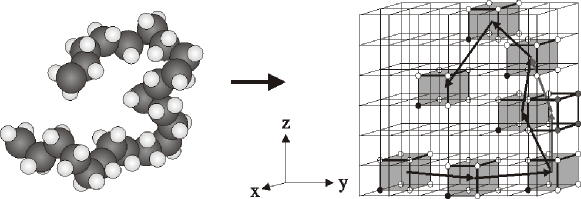
Figure 2: Bond fluctuation method. Polymer conformations are modeled by a chain of cubes on a cubic lattice and dynamics is obtained by random hops of the cubes on the lattice as indicated by the open cube on the right.

For the mono-disperse networks, mono-disperse melts of $M$ chains of length $N=16,...,256$ (cf. Table 1) monomers were equilibrated on a lattice of $128^{3}$ lattice sites at occupation density $\phi=0.5$ in periodic boundaries. The equilibration time was chosen such that at least 5 relaxation or reptation times per chain [29] could be realized. Afterward, $M/2$ of 4-functional cross-links were inserted and relaxation of the chains continued. A reaction took place whenever a free chain end diffused into the nearest possible separation to a cross-link that was not yet fully reacted. The reactions were stopped at 95% degree of end-linking in order to obtain samples with similar density of elastically active material.

Two more series of simulations are derived from using identical copies of the mono-disperse networks with $N=16$, 64, and 256 as initial conformations. These copies were relaxed for $2\times 10^{7}$ Monte-Carlo steps (MCS) whereby excluded volume was maintained for one series but the same extended bond vector set as in Ref. [30] was used to allow the strands to cross. For the other series, excluded volume was switched off and thus, simultaneously all entanglements. In order to provide an intuitive distinction between these different network types, these networks are called “phantom” (no excluded volume, no entanglements), “crossing” (no entanglements but excluded volume), or “entangled” (entanglements and excluded volume) throughout this work. Note that only the “phantom” networks correspond to the phantom network model and that only the segments of these networks are indeed Kuhn segments; the discussion of the “crossing” networks in the following sections requires additional corrections [31] due to the incompletely screened excluded volume of the monomers.

$N$	$M$	$n$	$bN_{p}^{1/4}$	$N_{p}$	$N_{c}$	$m$	$\phi_{\mbox{ac}}$	$z$
16	8192	2.32	4.45	8.2	6.5	0.068	0.878	0.413
32	4096	3.40	4.80	11.1	9.1	0.044	0.878	0.400
64	2048	4.47	4.94	12.4	11.4	0.032	0.882	0.389
128	1024	5.53	4.96	12.6	12.5	0.023	0.888	0.367
256	512	6.16	4.96	12.6	13.2	0.017	$\approx 0.91$	0.368

Table 1: Networks contain $M$ chains of $N$ monomers. $bN_{p}^{1/4}$ and virtual chain length $n$ are determined from Figure 9. The length of a correlated tube section $N_{p}$ is computed using $b=2.63$. The weight fraction of active material $\phi_{\mbox{ac}}$ is used to extrapolate towards a perfect network with no defects. For $N=256$, $\phi_{ac}$ is corrected for the incompletely relaxed dangling chains to obtain an improved extrapolation. $m$ is the average RBO of chains between junctions with 4 active connections to the network. The confinement length $N_{c}$ is is determined in Figure 10 from the average RBOs as function of $k$. $z$ is a single parameter fit of this data using equation (26).

The poly-disperse samples were obtained from mono-disperse melts of 256 chains of 512 monomers using the same density, lattice size, and boundary conditions as above. The melt was relaxed for $10^{9}$ simulation steps, which is about five reptation times [29]. Afterward either 7876 or 1732 monomers were inserted into the melt to model two-functional cross-links. The mixtures were relaxed for another reptation time of the chains without crosslinking. Ten conformations equally separated in simulation time were selected as starting point for the cross-linking reactions. Here, cross-linking was allowed for any monomer of the chains under three additional restrictions as in a previous work [27, 28]: each chain monomer can undergo only one reaction, the number of reactions is limited to two for the cross-links, and two consecutive monomers along one chain are not allowed to react with the same cross-linker. For each of the 20 samples, a degree of 100% cross-linking was achieved rapidly. The number average strand lengths in the sample is approximately $N\approx 8$ and 32 monomers. The number average length of active strands is about $8$ and 35 monomers while the weight average active strand length is about $14$ and 74 monomers respectively. Since the weight average strand length determines the sample average quantity of active segments, the samples are characterized below by using the weight average number of segments per active strand.

For data analysis, network conformations were recorded at a sampling time interval $\Delta t$ of $10^{5}$ MCS for a period of $10^{8}$ MCS (all networks with average strand length $N\leq 128$) and $2\times 10^{8}$ simulation steps for all other samples. This increased the accuracy of the entangled data for $N=256$ as compared to our previous study [1]. Diffusion of the sample was corrected by subtracting the motion of the center of mass for the analysis of monomer fluctuations. RBOs were computed from time averaged monomer positions.

3 Ideal networks: affine and phantom network model

3.1 Theory

Notation: square brackets $\left[\right]$ are used in the sections below to denote ensemble averages, angle brackets $\left\langle\right\rangle$ display time averages, bold letters like $\mathbf{R}$ represent vectors and double arrows $\overleftrightarrow{S}$ indicate tensors. All distribution functions are normalized such that the integral over all events is one.

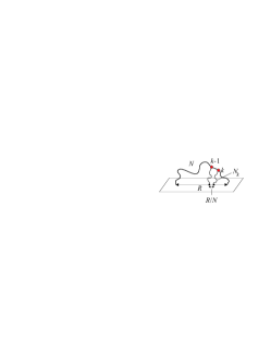
Figure 3: Affine network model. A polymer chain of $N$ segments (black curve) is fixed at both ends to the non-fluctuating elastic background (plane at bottom) at distance $R$. Fluctuations of the monomers (red spheres) around the time averaged monomer positions (black dots) can be modeled by virtual chains $N_{k}$ (dotted lines).

Let us assume a Gaussian distribution

$$P(N,\mathbf{R})=\left(\frac{3}{2\pi Nb^{2}}\right)^{3/2}\exp\left(-\frac{3\mathbf{R}^{2}}{2Nb^{2}}\right)$$ (3)

for the probability density of the end-to-end vector $\mathbf{R}$ of a chain made of $N$ segments, each with a root mean square length $b$ in three dimensional space. We further assume that there are no correlations among neighboring segments (freely jointed chain). Finally, we label the segments by $k$ from 1 to $N$ and move the origin of the coordinate system to the beginning of segment 1.

For the following discussion we use the concept of virtual chains to describe the time average monomer fluctuations in space. Consider a monomer that is part of a network of Gaussian chains. Due to network elasticity, the monomer fluctuates around a time average position in space. Because of the Gaussian nature of the chains, this fluctuation can be described by a harmonic potential or, alternatively, by the distribution of the end-to-end vectors of a “virtual” Gaussian chain of a particular number of segments that is fixed at the average monomer position in space. Note that below all monomer fluctuations are expressed by the length of the corresponding virtual chains to simplify the analysis.

3.1.1 Affine network model

In the affine network model, ideal chains are assumed to be attached to the so-called “non-fluctuating elastic background” [2] that deforms affinely with macroscopic deformations of the sample, see Figure 3. The long time average of all $N$ segments is given by the straight line connecting the fixed ends of the chain, $\mathbf{R}$. In this limit, all time averaged segments have the same orientation and length due to the constant force acting along the chain. Therefore, we obtain for the time average vector of any segment $k$

$$\left\langle\mathbf{b}_{k}\right\rangle=\mathbf{R}/N.$$ (4)

The fluctuations of monomer $k=1,...,N-1$ attached to Segments $k-1$ and $k$ can be computed by solving the Rouse matrix of the network chain. As a result one finds [4] that the time average monomer fluctuations are equivalent to the fluctuations in space of the endpoint of a virtual chain of

$$N_{k}=k(N-k)/N$$ (5)

monomers that is attached with its other end at position $\left\langle\mathbf{R}_{k}\right\rangle=k\mathbf{R}/N$ to the non-fluctuating elastic background. Therefore, the time average root mean square fluctuations $\sqrt{\left\langle\Delta R(k)^{2}\right\rangle}$ of monomer $k$ around its average position $\left\langle\mathbf{R}_{k}\right\rangle$ can be described by a virtual chain of $N_{k}$ segments,

$$\sqrt{\left\langle\Delta R(k)^{2}\right\rangle}=\left\langle\left(\mathbf{R}_{k}(t)-\left\langle\mathbf{R}_{k}\right\rangle\right)^{2}\right\rangle^{1/2}=bN_{k}^{1/2}.$$ (6)

The residual bond orientation $m_{k}$ of segment $k$ (RBO, also called the “vector order parameter” [12, 32]) can be defined via an auto-correlation function of the bond orientations, whereby averages need to be taken over a large number of initial conformations, see ref. [32]. $m_{k}$ can be computed also from considering the time average position of the monomers at the ends of Segment $k$

$$m_{k}=\left(\left\langle\mathbf{R}_{k}\right\rangle-\left\langle\mathbf{R}_{k-1}\right\rangle\right)^{2}/b^{2}.$$ (7)

Note that equation (7) is the most precise way of measuring $m_{k}$ from a given set of conformations and it is mathematically equivalent with considering any available conformation as initial conformation for the averaging of the auto-correlation functions.

The time average conformation of an ideal chain with fixed ends in the limit of an infinitely long sampling interval $\Delta t\rightarrow\infty$ is given by the straight line connecting both chain ends, cf. Figure 3. Because of equation (4) we obtain for this limit

$$m_{k}=\frac{\left\langle\mathbf{b}_{k}\right\rangle^{2}}{b^{2}}=\frac{\left\langle\mathbf{R}^{2}\right\rangle}{b^{2}N^{2}}.$$ (8)

Let us now discuss mono-disperse networks with uniform strand length $N$ between the junctions. If we insert the ensemble average of the Gaussian distribution, $[\mathbf{R}^{2}]=b^{2}N$, into equation (8), we find for the ensemble average of the RBO

$$[m_{k}]=N^{-1}$$ (9)

independent of $k$. The distribution of RBOs is, therefore, fully determined by the length distribution of end-to-end vectors of the $N$-mers

$$P(N,R)4\pi R^{2}\mbox{d}R=4\pi R^{2}\left(\frac{3}{2\pi Nb^{2}}\right)^{3/2}\exp\left(-\frac{3R^{2}}{2Nb^{2}}\right)\mbox{d}R.$$ (10)

Substituting $m=R^{2}/(b^{2}N^{2})$ we can transform this probability density into a probability density of RBOs for Gaussian chains (the so-called “Gamma distribution”):

$$P(N,m)2\pi m^{1/2}b^{3}N^{3}\mbox{d}m=N^{3/2}\sqrt{\frac{27m}{2\pi}}\exp\left(-\frac{3mN}{2}\right)\mbox{d}m.$$ (11)

This distribution was used in previous works to fit experiment and simulation data. The agreement between equation (11) and the data was often poor, in particular for dry networks [32].

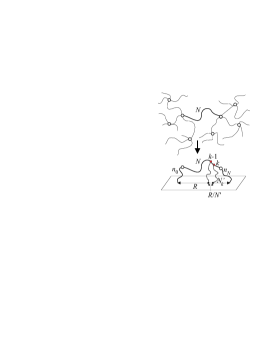
Figure 4: Reduction of ideal phantom network (top) to the corresponding affine chain (bottom, cf. Figure 3). The virtual chains $n_{0}$ and $n_{N}$ model the fluctuations of the cross-links (white spheres), if the $N$-mer in between is removed.

It has been shown [32, 33, 34] for Gaussian chains with fixed ends that the residual coupling constant $s_{k}$ as obtained in multi-quantum NMR experiments is related to the RBO via

$$s_{k}=\frac{3}{5}m_{k}.$$ (12)

Moreover, the scaling predictions for $s_{k}$ and $m_{k}$ as function of time are identical in the entangled regime (cf. section 10). Therefore, $s_{k}\propto m_{k}$ for non-entangled and entangled chains and all scaling laws derived for the RBO apply also for the experimental data of dry networks.

3.1.2 Phantom network model

In the phantom network model, one assumes that restrictions to junction fluctuations result exclusively from the network connectivity [2, 35, 36]. In general, this would require to solve the Rouse matrix of the entire network, which is impossible for networks of unknown connectivity (as in experiments) and can be done only numerically for randomly connected networks (simulations). Therefore, we use the standard approximation of an ideally branching network structure and the resulting predictions for the phantom network model to derive an analytical expression. In general, the phantom model description for a given network chain can be reduced [2] to a combined chain of

$$N^{\prime}=n_{0}+N+n_{N}$$ (13)

segments, for which the virtual chains $n_{0}$ and $n_{N}$ model the cross-link fluctuations at both ends of the $N$-mer, after the $N$-mer has been removed from the network [2]. The combined chain $N^{\prime}$ is attached with its ends to the non-fluctuating elastic background. Therefore, we can rewrite all results of the affine model using $k^{\prime}=n_{0}+k$ instead of $k$ and $N^{\prime}$ instead of $N$. To distinguish between affine and phantom model in the equations we indicate below all quantities related to the phantom model by an apostrophe. For instance, the monomer fluctuations in space are described by virtual chains $N_{k}^{\prime}=k^{\prime}(N^{\prime}-k^{\prime})/N^{\prime}$. These modifications lead to

$$[m]=N^{\prime-1}=\frac{f-2}{f}N^{-1},$$ (14)

whereby the right equation only holds for the case of a perfect [37] $f$-functional network of mono-disperse chains $N$ [4]. In the phantom model (as in the affine model), the average residual RBO is proportional to the inverse of the elastic strand $N^{\prime}$. Note that network defects will show a clear effect on the local distribution of $m$ in the framework of the phantom model, since any defect will lead to a local variation of the cross-link fluctuation and $N^{\prime}$. In order to reduce this additional degree of complexity, we restrict the data analysis below to strands that are connected at both ends to cross-links with four active connections to the network. As can be deduced from the derivation of the above right equation in ref [4], this procedure removes the largest corrections due to imperfect network structure for networks with a low average degree of imperfection.

3.2 Comparison with simulation data

For the phantom and crossing networks having N = 16 and 64, Figure 5 shows plots of the mean square monomer fluctuations against the position k along the chain. The data are normalized by the root mean square bond length $b^{2}$. Thus, the ordinate in Figure 5 displays the number of segments $N_{k}^{\prime}$ in the corresponding virtual chain that models the fluctuations of monomer $k$. For the phantom networks, we find excellent agreement for the $k$-dependence when the length of the virtual chains $n_{0}$ and $n_{N}$ was adjusted to fit the data. The length of the virtual chains, however, shows some interesting finite size effect, which is discussed in section 10.2.

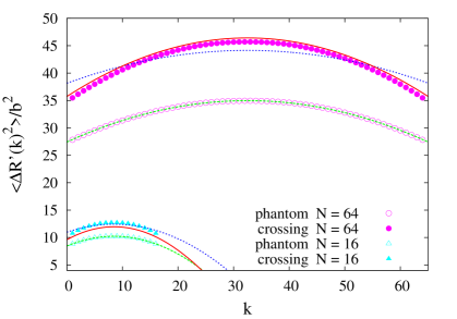
Figure 5: Mean square monomer fluctuation as function of monomer position $k$ along the chain for phantom and crossing networks of different $N$. Dashed green line and dotted blue lines: fit with phantom model. Red continuous line: phantom model prediction combined with excluded volume correction.

Another interesting observation is that the data of the “crossing” networks show a different $k$-dependence as predicted by the phantom network model in Figure 5. This is visible in the different curvature of simulation data and theoretical prediction. In particular, we find clearly enhanced time average fluctuations of the monomers in networks with excluded volume, even though the dynamics is slowed down as compared to the phantom simulations. This behavior indicates that a lower extensional force is required to stretch the chains with excluded volume. The different curvature of the simulation data and the phantom model prediction further indicates that the force is not lower by a constant factor, instead, the effective force reduction must be a function of the internal distance along the chains.

Both observations are in line with previously observed corrections to ideal chain conformations in dense melts [31] that arise from the incompletely screened excluded volume at short distances along the chains. This is commonly associated with the bare excluded volume of the monomers [6], but was also identified with the bulk modulus effectively measured for those systems [38]. In order to test whether this effect accounts for the differences between the phantom and the crossing data, we perform the following test: the fit results of the phantom simulations are used as input for the virtual chain lengths. The phantom prediction for fluctuations is corrected as described at equation (10) in ref [38] by a factor of

$$\frac{\left\langle\Delta R(k)^{2}\right\rangle}{\left\langle\Delta R^{\prime}(k)^{2}\right\rangle}\approx\frac{b_{e}^{2}}{b^{2}}\left(1-\frac{c_{e}}{\sqrt{N_{k}^{\prime}}}\frac{b_{e}}{b}\right)$$ (15)

with parameters $b_{e}\approx 1.23b$ and $c_{e}\approx 0.41$ as reported in [38]. The result is shown in Figure 5 as continuous red line. We observe good agreement with the simulation data, when considering that the phantom and crossing data are collected from two independent simulation runs of two networks with same connectivity but with and without excluded volume interactions respectively. In consequence, Figure 5 leads to the proposal that the estimate for the phantom contribution to network modulus should be corrected for real networks with respect to the effect of excluded volume, since the screening of excluded volume does not depend on entanglements [38]. Furthermore, we use equation (15) below to correct the effect of incompletely screened excluded volume for the entangled samples.

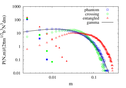
Figure 6: Distribution $P(m)$ of the RBO for phantom networks, crossing networks, and regular networks of $N=16$. The gamma distribution at equation (11) was fitted with variable $N^{\prime}$ to the phantom data. Open symbols show results of active network chains between two junctions that connect 4 active strands. Full symbols show the results of dangling chains.

The distribution of the RBO $P(m)$ of equation (11) is compared with simulation data of the shortest networks $N=16$ at Figure 6. A fit with a variable chain length $N^{\prime}$ as only parameter yields an apparent $N^{\prime}=27.5\pm 0.1$. The monomer fluctuation data, however, would suggest a clearly larger $N^{\prime}\approx 17+2\cdot n_{0}\approx 41$ (see section 10.2 for $n_{0}$). This discrepancy can be removed when considering that the ratio $R^{2}/N^{2}$ enters in computing the RBO, cf. equation (8). We find that the average square end-to-end vectors are enlarged by approximately $40\%$ as compared to the ideal prediction $R^{2}=b^{2}N$, which is roughly in agreement with equation (15). Note that the phantom networks were originally entangled networks for which the excluded volume was switched off. Apparently, the enlarged state of the chains at crosslinking is conserved by the fixation of the network via the periodic boundary conditions. Taking into account this enlarged chain size, we find $N^{\prime}\approx 39$ from the distribution function of RBOs. This result is in reasonable agreement to the $N^{\prime}\approx 41$ as obtained from the analysis of monomer fluctuations.

Figure 6 also shows that there are only small differences concerning the distribution of RBOs for “phantom” networks as compared to “crossing” networks. The latter show a slightly enlarged average RBO with a weak depletion at small $m$. This depletion can be explained by the soft repulsion of connected active junctions via the excluded volume of all monomers attached to these junctions. The data of entangled networks in Figure 6 is clearly shifted compared to both non-entangled model networks. Also the dangling material of the “network” data shows a distinct delay concerning relaxation as compared to non-entangled models. Both observations are remarkable, since strands of 16 monomers are clearly shorter than previous estimates for the entanglement length, which amounted in 30 monomers or larger [29, 39]. The clear shift of the dangling chain data indicates that a similar analysis of experimental data can separate inactive parts of the network, if a possible peak at smallest RBOs is excluded.

The RBO is averaged for segments of same $k$ and plotted as function of $k$ in Figure 7 for the “crossing” and “phantom” networks. The simulation data of the “phantom” networks shows that the RBO is independent of $k$ as predicted by equation (8). The phantom model predicts for a perfectly branching (no finite loops) network with weight average active functionality $f_{a}$ of the junctions that

$$m_{k}N=N^{\prime-1}N\approx(f_{a}-2)/f_{a}.$$ (16)

As discussed in section 10.2, $f_{a}$ in the networks is increasing with $N$ and also, the average chain size grows as function of $N$ due to preparation conditions (entangled network with excluded volume switched off after crosslinking) as discussed above. This explains the increasing $Nm_{k}$ for larger $N$.

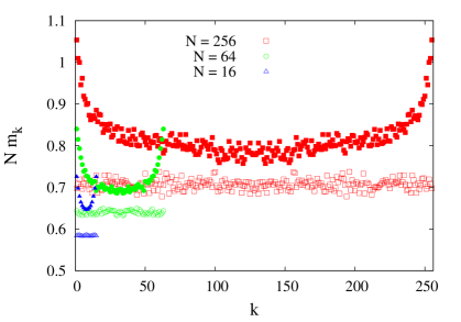
Figure 7: $m_{k}$ as function of the position $k$ along the chain. Results are multiplied by $N$. Open symbols show data of phantom networks, filled symbols data of crossing networks.

For the “crossing” simulations, we find an enhancement of RBOs close to chain ends in the range of $15-30\%$ compared to the middle of the chains. This enhancement is attributed to the enlarged excluded volume interactions near the cross-links. Interestingly, the RBO remains larger as the phantom prediction in the middle of the chains. A close inspection of the simulation data revealed that the time average monomer positions of an active chain are not exactly (beyond statistical error) following a straight line between the two cross-links attached to both ends. We argue that overlapping chains are competing for the same lattice positions. This leads to a weak distortion of the average monomer positions as compared to the phantom networks. Therefore, an enlarged RBO is detected.

In summary of this section we find excellent agreement between the “phantom” networks and the predictions of the phantom model. The “crossing” networks show additional effects of excluded volume, which lead to increased monomer fluctuations and weakly enhanced RBOs, in particular close to chain ends. Therefore, the phantom model can be used as a first order approximation to develop a model for the average segment orientations of entangled networks. Corrections due to excluded volume for monomer fluctuations will be introduced below where necessary.

4 Entangled networks: average segment orientations

The problem that is analyzed in this section is depicted in Figure 8: entanglements confine the motion of monomer $k$ to a small region in space that might be shaped like a tube. Since this “tube” is not perfectly straight and monomer $k$ can move a large distance along this curved object, the average monomer positions neither fall on the primitive path (the center line of the confining potentials) nor onto the straight line connecting the cross-link positions as in the affine or phantom model (cf bottom of Fig. 8). The RBOs, however, are related to the vector connecting the time average monomer positions. We shall see that the RBO reflects the contour of the primitive path as averaged by the motion of the monomers along the confining tube. How this can be analyzed from computer simulations and experimental data are discussed in the present section.

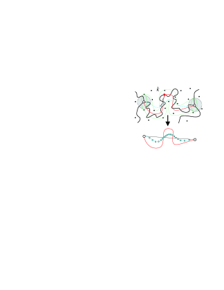
Figure 8: Upper part: Black dots show schematically entanglements with active strands that dynamically fluctuate in space with time. White spheres show cross-links, the gray volume represents a typical fluctuation volume of a crosslink. Black lines show polymer strands, the imaginary surrounding time average tube of the chain in the middle is sketched by the green lines, while the primitive path of the tube is given by the red line. Monomer $k$ (red sphere) fluctuates mainly along this curved tube leading to an average monomer position (blue sphere) that is not located on the primitive path. Lower part: Time average positions of all monomers (blue spheres) are compared with primitive path (red line) and end-to-end vector of the chain.

4.1 Theory

For our derivation, we use three assumptions that are consistent with a slip-tube model for rubber elasticity [2]:

1. The motion of the monomers is confined to a tube like region in space.

2. The primitive path of the tube performs a random walk in space.

3. The segments of the chains can slide along the contour of the tube, whereby the motion along the chain is limited by network connectivity (as described by the phantom model), while the perpendicular motion is limited by entanglements.

In entangled polymer networks with a degree of polymerization $N$ of the network strands larger than the entanglement degree of polymerization $N>N_{e}$, the monomer and cross-link fluctuations are additionally constrained as compared to phantom networks by entanglements with neighboring strands. In the framework of the tube model, this is typically expressed by a confining potential that restricts perpendicular fluctuations of the polymers to a tube like region in space [5], see Figure 8. In analogy to a stretched polymer [6], we use $N_{c}$ to describe the diameter of the tube

$$a\approx bN_{c}^{1/2}$$ (17)

(cf. the introduction). Within the frame of reference of the tube (primitive path), the chains have an average end-to-end distance [6] given by

$$\left[L\right]\approx aN/N_{c}\approx bN/N_{c}^{1/2}.$$ (18)

Let us consider first an entirely straight tube and use the index t to denote the frame of reference of the tube. For simplicity, we use the phantom model for a chain of $N^{\prime}=N+n_{0}+n_{N}$ monomers to describe the motion of the monomers along the tube (which is not confined by the tube potential) by a virtual chain length $N^{\prime}_{k}$, see equation (5). The ends of the combined chain $N^{\prime}$ are, thus, attached to the elastically active background at $x_{0,t}=0$ and $x_{N^{\prime},t}=\left[L\right]N^{\prime}/N$ in order to satisfy equation (18). The probability of finding monomer $k$ at positions $x_{t}$ along the tube is computed by the one-dimensional contribution [4] of the three dimensional Gaussian distribution

$$P_{t}(k,x_{t})\approx\sqrt{\frac{3}{2\pi b^{2}N^{\prime}_{k}}}\exp\left(-\frac{3\left(x_{t}-\left\langle x_{k,t}\right\rangle\right)^{2}}{2b^{2}N^{\prime}_{k}}\right),$$ (19)

whereby $\left\langle x_{k,t}\right\rangle=\left[L\right](n_{0}+k)/N^{\prime}$ is the average position of monomer $k$ in the coordinate system of the tube.

It is typically assumed that the tube performs a random walk in space [6] whereby the step lengths cannot exceed the tube diameter for maintaining random walk statistics of the full chain. The fluctuations of inner monomers of entangled chains with $N^{\prime}_{k}\gg N_{\mbox{\emph{p}}}$ are dominated by fluctuations along the tube [4], while the motion of monomers with $N_{k}\lesssim N_{p}$ remains essentially isotropic. The reptation like motion of monomer $k$ along the tube is limited by the virtual chain length $N^{\prime}_{k}$. Therefore, for long chains with $N^{\prime}_{k}\gg N_{p}$, the time average root mean square fluctuations of monomer $k$ in space are approximately

$$\sqrt{\left\langle\Delta\mathbf{R}_{en}(k)^{2}\right\rangle}\approx bN_{p}^{1/4}N^{\prime}{}_{k}^{1/4}.$$ (20)

It is important to point out that in the limit of very long entangled chains, $N^{\prime}_{k}\gg N_{p}$, the monomer fluctuations are only related to the correlation length of the primitive path and not to the tube diameter, since the contribution of the fluctuations perpendicular to the tube axis become ignorable. Note that the above relation is used to estimate $N_{p}$ from monomer fluctuations.

Along a perfectly straight tube, the RBO of an entangled chain stretched to $\left[L\right]$ adopts a value of $m=1/N_{c}$ and the RBO is proportional to stress as mentioned in the previous discussion about the affine model. Bonds that fluctuate along a curved tube of length $\left[L\right]$ sample tube sections of different orientations. The sampling of different tube orientations reduces the average RBO of the segments. In order to obtain an analytical solution, the orientation correlation between the tube sections at position $x_{t}$ and at the average monomer position $\left\langle x_{k,t}\right\rangle$ along the tube is approximated by an exponential decay for the tube orientation $O_{t}(x_{t})$

$$O_{t}(x_{t})\approx\exp\left(-|x_{t}-\left\langle x_{k,t}\right\rangle|/c\right),$$ (21)

with decay length $c\approx bN_{p}^{1/2}/2$. The resulting reduction in RBOs from $1/N_{c}$ due to tube curvature is obtained by integrating $\int_{-\infty}^{\infty}P_{t}(k,x_{t})O_{t}(x_{t})dx_{t}$. This yields

$$m(N,k)\approx\frac{1}{N_{c}}\cdot e^{y^{2}}\cdot\mbox{erfc}\left(y\right)$$ (22)

with the complementary error function [40] $\mbox{erfc}(y)$ and

$$y^{2}=2N^{\prime}_{k}/3N_{p}.$$ (23)

We expect $N_{c}\propto N_{p}\propto N_{e}$ in the limit of $N_{k}\rightarrow\infty$. Thus, one obtains as asymptotic result

$$m\propto N^{-1/2},$$ (24)

for the center monomers in long chains. Since the different RBO near the chain ends leads to a contribution of order $N^{-1}$, we expect that equation (24) holds for average RBO of active network strands.

The result of equation (24) is clearly different from the predictions of the affine or phantom network model with $m\propto N^{-1}$ or $m\propto N^{-1}+N_{e}^{-1}$ that both are obtained under the assumption [16, 41] that the RBO must be proportional to the modulus of the network, $m\propto G$.

4.2 Comparison with simulations and experiment

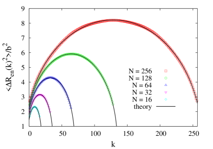
Figure 9: Mean square monomer fluctuations in entangled networks as function of monomer position $k$ along the chain normalized by the square bond length $b^{2}$. The theoretical lines are fits of equation (20) with $N_{p}$ as single adjustable parameter, since the crosslink fluctuations as given by $n_{0}$ can be determined independently. The results for $N_{p}$ are given in Table 1.

Similar to the previous section, only active network strands connecting pairs of cross-links with 4 active connections are analyzed. This restriction is necessary, since crosslinks with a smaller number of active strands show larger fluctuations at the chain ends.

The $N^{\prime}{}_{k}$ dependence of eq. (20) reproduces well the monomer fluctuations as function of $k$ in all samples. The cross-link fluctuations as approximated by the virtual chain length $n=n_{0},n_{N}$ (cf. Table 1) grow clearly weaker than the phantom prediction $\sim N^{1/2}$, remain smaller than $N_{c}$, but do not yet fully saturate for large $N$. This is to be expected, since active cross-links join $\geq 3$ active chains. Thus, the fluctuations of active cross-links in an entangled network must be limited to a volume $V\lesssim a^{3}.$ The fit parameter $bN_{p}^{1/4}$ seems to converge towards 4.96 for large $N$. The reduction of this parameter for small $N$ is possibly the result of the beginning transition to the non-entangled regime and could be related to a tighter trapping of active chains for small $N$. Note that the mean square monomer fluctuations of the crossing and phantom networks are much larger (cf. Figure 5) and follow a different $N^{\prime}_{k}$ dependence.

The good agreement between simulation data and theory in Figure 9 is rather surprising. Apparently, there are two opposite corrections that largely cancel each other. First, as discussed around equation (15), the incompletely screened excluded volume interactions enlarge monomer fluctuations. This can be modeled by an effective bond length $b_{e}$ with $b_{e}^{2}/b^{2}\approx 1.5$ for the bond fluctuation model at polymer volume fraction $\phi=0.5$ [38]. According to the results of the crossing networks above, we expect similarly increased apparent fluctuations in networks (since the end monomers are connected to several chains, the apparent $b_{e}^{2}/b^{2}$ is expected to be $\gtrsim 1.5$). Second, we know that $n<N_{c}$ and thus, the monomers attached to the cross-links fluctuate rather isotropically, while fluctuations of inner monomers $N_{k}\gg N_{p}$ are dominated by the fluctuations along the tube. In this limit, only one directional component contributes to fluctuations. Thus, we expect that the measured square fluctuations in the coordinate system along the tube for chains $N\gg N_{p}$ converge to 1/3 of the unconstrained isotropic fluctuations. This leads to a reduction of the measured square fluctuations in Figure 9 of approximately $3^{1/2}\approx 1.7$ for very long $N$. Both corrections converge as function of $N^{\prime}{}_{k}^{1/2}$ towards the limiting behavior for inner monomers for large $N$. According to the above numerical estimate, most of these corrections cancels each other. Since, we also do not observe significant differences between theory and simulation data, we conclude that $N_{p}$ can be calculated via equation (20) without the need of additional corrections or a numerical constant. However, for a different simulation method with a clearly different $b_{e}/b$, a correction could become necessary.

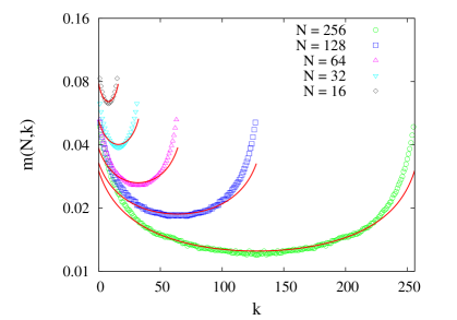
Figure 10: Average RBO as function of monomer position $k$ along the chains. Theoretical lines are fits with equation (22) with $N_{c}$ as parameter and including the corrections for enlarged chain size and fluctuations as described in the text. The results for the fit of $N_{c}$ are given in table 1.

The RBO $m(N,k)$ is analyzed as function of bond index $k$, see Fig. 10. We use the same subset of active chains and parameters $n$ and $N_{p}$ as in Figure 9. As discussed for the crossing networks in the previous section, the partially expanded chain conformations (due to the incompletely screened excluded volume) need to be corrected. This leads to a) an enlargement of the average square chain extension, and thus, we obtain an additional factor of approximately $b_{e}^{2}/b^{2}\left(1-c_{e}b_{e}/(b\sqrt{N}\right)$ for predicting the RBO in equation (22). b) As shown in the previous chapter, monomer fluctuations along the tube, as given by $N^{\prime}_{k}$, are enlarged by $b_{e}^{2}/b^{2}\left(1-c_{e}b_{e}/(b\sqrt{N^{\prime}_{k}}\right)$. This can be corrected for in equation (23). c) $N_{p}$ requires no modification according to the discussion of the preceding section. Equation (22) including these corrections is fitted to the innermost 80% of the data of each network in Figure 10 using $N_{c}$ as the only adjustable parameter. The data near the ends is discarded due to the extra contribution from excluded volume as shown in Figure 7. The result for $N_{c}$ is summarized in Table 1 and both $N_{c}$ and $N_{p}$ are plotted in Figure 11. We find that both $N_{p}$ and $N_{c}$ are increasing and converge for $N\rightarrow\infty$ to the asymptotic limit as proposed in the introduction. Figure 11 indicates that $N_{c,\infty}/N_{p,\infty}\approx 5/4$, which agrees with the result $N_{p}\leq N_{c}$ of Helfand et al. [22, 23].

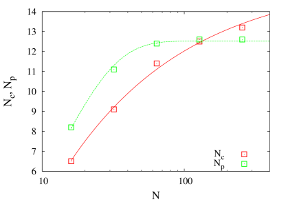
Figure 11: $N_{c}$ and $N_{p}$ as function of $N$. The lines are the approximations for the convergence towards the asymptotic limit, equation (1) and (2), as discussed qualitatively in the introduction.

In our previous work [1] we did not distinguish between $N_{p}$ and $N_{c}$ and omitted the above corrections for fluctuations and expansion in chain size. As a result, a fit of the data suggested a decreasing de-correlation length for larger $N$. The present analysis shows, that this observation was caused by the neglect of the above corrections for chain size and monomer fluctuations.

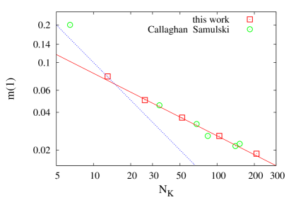
Figure 12: Average RBO of active chains as function of the number of Kuhn segments $N_{K}$ extrapolated to networks without defects. The continuous red lines correspond to a fit with power law $m\propto N^{-1/2}$ while the blue dotted line shows $m=N^{-1}$. The experimental data are taken from Ref [17] and normalized as described in the text.

The average RBO $m$ is analyzed as function of the number of Kuhn monomers $N_{K}$ in Figure 12 and compared with the experimental data of table 1 of Ref [17]. In order to superimpose both data sets, we compute the number of Kuhn segments $N_{K}=Nb/b_{e}=N/1.23$ with $b_{e}$ of Ref [38] for the simulation data and use the molar mass of a Kuhn Monomer for PDMS $M_{0}=381g/mol$ from Ref [4] for the experimental data. Next, we extrapolate the average RBO to networks without defects by computing $m(1)=m/\phi_{ac}^{2/3}$ for both simulations and experiment. Finally, we shift the experimental data for the residual moment along the ordinate (here: by a factor of $1/30000000$) to optimize the overlap of the data in the large $N_{K}$ region. This is to test, whether there is a qualitative agreement between simulations and experiment for entangled networks. This comparison is possible, since in bulk materials, the residual moment is $\propto s\propto m$ as discussed in Ref [32]. Note that the perdeuterated sample of Ref [17] is left out from the plot (similar to the analysis of Ref [17]) due to its different relaxation behavior. If we ignore the two data points for the smallest chain lengths in Figure 12, we find that both simulation and experimental data of Ref [17] follow the predicted scaling of $N^{-1/2}$ over about one decade in $N_{K}$. This observation is in contrast to the proposal of Refs [16, 41], which related the RBO to the equivalent length $N_{el}$ of an elastic chain describing the network elasticity in the framework of the affine model:

$$m\propto\frac{1}{N_{el}}=c\left(\frac{1}{N}+\frac{1}{N_{e}}\right)$$ (25)

using a normalization constant $c$. Note that in Ref [17] it was attempted to use equation (25) to describe the RBO as function of $N$. But this lead to a different power for $m$ as function of $N_{el}$ as proposed in equation (25).

Let us now discuss the experimental data in more detail. The location of the cross-over between the entangled and the non-entangled regimes may be estimated by assuming that the data point at smallest $N_{K}$ is clearly in the $N^{-1}$ regime of non-entangled networks. If we use this data point to fix the $N^{-1}$ regime, the crossover to the $N^{-1/2}$ is around $22$ Kuhn monomers. Since $N_{e}\approx 32$ for PDMS [4], we estimate $N_{p}\approx 2N_{e}/3$. If we assume that $N_{p}$ is of the order of the average weight between two slip links, this result is close to the prediction $N_{p}/N_{e}=4/7$ of Ref [2] or near the estimates $1/2$ of Ref [21] and $4/5$ of Ref [20]. This agreement supports that our model may be used for a refined quantitative analysis of entangled polymers.

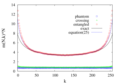
Figure 13: Average RBOs for all mono-disperse networks with $N=256$ multiplied by $N$. Comparison of equation (26) and exact solution (equation (22)) with the data of entangled networks (red circles). For comparison, the data of the non-entangled two model samples is also included.

In Fig 13 we compare data of the phantom, crossing, and entangled networks with $N=256$ in order to show the clear qualitative and quantitative differences for the entangled networks. In particular, the strong increase of the RBO towards the chain ends is characteristic for entangled networks. Note that this behavior is supported by experimental data of Gronski et al. [42, 43], who determine a clearly enhanced RBO close to cross-links as compared to inner parts of the chains.

Let us now try to find a simplified approximation for the RBO as function of $k$. We expect $m(k)$ to be reduced by a factor proportional to the return probability to the most probable tube section $\sim\left(N_{p}/N^{\prime}_{k}\right)^{1/2}$ as compared to the the straight tube result $1/N_{c}$, since all neighboring uncorrelated tube sections are averaged to zero. Furthermore, we ignore the corrections for increased chain size and enlarged fluctuations. For the remaining approximation, we introduce a numerical constant $z$ to fit the data in Fig. 10 by

$$m_{k}\approx\frac{z}{\sqrt{N_{p}N^{\prime}_{k}}}.$$ (26)

This approximation works surprisingly well as shown at Fig. 13 and even compensates some deviations near the chain ends. The resulting $z$ vary less than $15\%$ over more than a decade of $N$ (see table 1). Note that we still require $N_{p}$ and the virtual chain length $n$ of table 1 as parameters that are independently determined from monomer fluctuations. We have to point out that any difference between $N_{c}$ and $N_{p}$, all corrections due to the extended chain conformations, enlarged monomer fluctuations, the numerical coefficients of equation (22) and (23) and all effects of the crosslinking process are summed up in $z$. A quantitative analysis of the RBO, therefore, requires the computation of the more detailed approach above. Nevertheless, we think that equation (26) is quite useful in practice, since it allows for a) a quick prediction of the average RBO as function of $k$ once $z$ has been determined for a particular $N$ at a particular polymer volume fraction (for a given polymer or simulation model). Furthermore, we use equation (26) as a simplification to derive the distribution of RBOs in the following sections.

5 The distribution of residual bond orientations in entangled networks

5.1 Theory

In the model developed above, we computed the average RBO as function of $k$ by assuming an average tube length $\left[L\right]$ and an average tube curvature as expressed by an exponential de-correlation function. This is a reasonable approximation for deriving the average RBO, but it requires further generalization for computing the distribution of the RBOs.

First, we have to clarify, that the approximation below focuses on intermediate chain lengths $N\gtrsim N_{p}$ as it is typical for polymer networks. For very long chains, any variation of the local tube curvature is averaged out (except of near the ends), since the monomers will visit a large number of different tube sections $\propto\left(N_{k}/N_{p}\right)^{1/2}\gg 1$ while moving back and forth along the tube. Also, the fluctuations in the tube length grow only $\propto\left(N/N_{p}\right)^{1/2}$ and thus, become unimportant for $N\rightarrow\infty$. Apparently, both corrections lead to a qualitatively similar broadening of the distribution of RBOs as function of $N$. Therefore, we discuss below only the effect of tube length fluctuations that is better documented in literature. We expect that the effect of fluctuations in the local tube curvature leads to an additional broadening of the RBO distribution.

Let us assume that cross-linking occurs rather instantaneously and that the relaxation of the network chains during cross-linking does not lead to a an equilibration of two connected tubes until the full network structure is fixed. Under these conditions, the frozen length distribution of the network tubes is roughly equal to the instantaneous length distribution of the ensemble of tubes inside the melt prior to cross-linking.

In the Doi-Edwards model [6], polymers in melts are considered as Rouse chains inside a tube, whereby the chain is stretched by a potential of entropic origin for keeping its extension at time average length $\left\langle L\right\rangle=[L]=bN/N_{c}^{1/2}$. We assume that the tube length distribution of the melt is frozen in the network. Assuming a quadratic approximation [44] for the free energy

$$F(L)=\frac{3\gamma kT}{2Nb^{2}}\left(L-\left[L\right]\right)^{2}$$ (27)

with an effective spring constant $\gamma$ of order unity we obtain normal distributed tube lengths [4] around $\left\langle L\right\rangle$ as described by

$$P(N,L)\mbox{d}L=\sqrt{\frac{3\gamma}{2\pi Nb^{2}}}\exp\left(-\frac{3\gamma(L-\left[L\right])^{2}}{2Nb^{2}}\right)\mbox{d}L.$$ (28)

The magnitude of the apparent spring constant could be modified in a network due to the impact of the local tube curvature, or due to stress equilibration and redistribution of monomers when connecting two tubes at their ends.

Comparing equation (26) with the result of a straight tube $m_{k}=1/N_{c}$ we can interpret the fluctuations along the curved tube as a length contraction of a straight tube by a factor $\beta=z^{1/2}\left(N_{p}/N^{\prime}_{k}\right)^{1/4}$, since $m\sim L^{2}$ in this case at constant $N$ and $b$ analogous to the affine model result $m\sim R^{2}$ at constant $N$ and $b$ (see previous chapter for parameter $z$). This leads to a contracted apparent tube length $\beta\left[L\right]$ and a modified spring constant of this “contracted” ensemble of chains $\gamma_{c}=\gamma\beta^{2}/z^{2}$. Thus, the monomer fluctuations along the tube let the distribution of the primitive path lengths appear contracted [45] for the analysis of the RBO:

$$P(L,k)\mbox{d}L=\sqrt{\frac{3\gamma_{c}}{2\pi N^{\prime}b^{2}}}\exp\left(-\frac{3\gamma_{c}(L-\beta\left[L\right])^{2}}{2N^{\prime}b^{2}}\right)\mbox{d}L.$$ (29)

Equation (29) can be transformed using the substitution $m=L^{2}/(b^{2}N^{\prime 2})$ to obtain the distribution of RBOs in entangled networks

$$P(m,k)\frac{bN^{\prime}}{2m^{1/2}}\mbox{d}m=\sqrt{\frac{3\gamma_{c}N^{\prime}}{8\pi m}}\exp\left(-\frac{3\gamma_{c}N^{\prime}}{2}\left(m^{1/2}-\beta/N_{p}^{1/2}\right)^{2}\right)\mbox{d}m.$$ (30)

This equation allows us to compute the distribution of RBOs for any labeled monomer $k$ and thus, for the full chain via the summation

$$P(m,N)\mbox{d}m=\sum_{k=0}^{N}P(m,k)\frac{bN^{\prime}}{2m^{1/2}}\mbox{d}m/(N+1).$$ (31)

Note that this summation runs over all $N+1$ segments between the cross-links, while the length distribution was determined by the combined chain $N^{\prime}$.

5.2 Comparison with simulation data

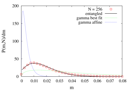
Figure 14: Distribution of RBOs in the entangled network $N=256$ (data points). The gamma distribution of equation (11) is plotted using $N=256$ (affine model) or fitted to the data yielding $N=25\pm 5$. The “entangled” line is computed using equation (31) with $\gamma=0.45\pm 0.05$ and the previously determined data of table 1 for $N_{p}$, $z$, and $n$.

The distribution of RBOs in the entangled network $N=256$ is plotted in Fig. 14. Neither the affine model (or the phantom model, not shown) nor a best fit using the gamma distribution with $N$ as adjustable parameter can even qualitatively describe the data. A best fit of the gamma distribution of equation (11) yields $N\approx 25$, which is clearly below $N=256$ and not in agreement with the $N_{p}$ as determined from monomer fluctuations. A fit of equation (31) using a variable $\gamma$ leads to a clearly better qualitative description of the simulation data as compared to the gamma distribution.

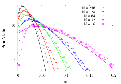
Figure 15: Distribution of RBOs in all entangled networks (data points). Full lines are computed using equation (31) with $\gamma=0.45$ and the data of table 1 for $N_{p}$, $z$, and $n$.

The data of all entangled networks of the present study is fitted with equation (31) at Figure 15 using a single spring constant $\gamma$ for all networks. In particular for large $N$ we find good agreement. For small $N$ we observe an additional depletion at small $m$. We attribute this difference to the effect of excluded volume: Since the cross-links are attached to four chains, the cross-links repel each other similarly to the centers of star polymers in a melt of stars. This removes extremely short tube lengths from the time averaged conformations and leads to the depletion at $m\approx 0$. Since the average tube length grows $\propto N$, the effect of this short distance correction vanishes for $N\rightarrow\infty$.

In the derivation above, we adopted a harmonic potential to derive the tube length distribution as introduced in the Doi-Edwards model for entangled polymers. The parameter $\gamma$ as front factor of this potential is considered to be close to 0.8 [4] as indicated by experimental data. Here, a good agreement is found at a rather constant $\gamma\approx 0.45$, which was used to compute all solid lines in Figure 15. If we accept the experimental $\gamma$ as reference, the reduced $\gamma$ of the present study indicates that the RBO distribution is additionally broadened, possibly by local fluctuations in tube curvature: in contrast to melts where diffusing chains continuously create and sample new tube sections, the fixed network chains sample only a particular set of tube sections and curvatures. This may explain our observations, but requires more detailed investigations to proof this claim.

6 Poly-disperse Networks

Following the discussion in section 5, we expect that the RBO parameter $m(N)$ of a strand of $N$ monomers in poly-disperse samples follow $m(N)\approx z/(NN_{p})^{1/2}$ for sufficiently large $N>N_{p}$. The data in Figure 16 clearly supports the predicted scaling. Note that all data points have been extrapolated to a density of 100% active material, since the weight fraction of dangling chains leads to a significant shift of the data. The data of the networks $N=14$ shows slightly enhanced order, probably due to a tighter trapping of the strands at the crossover to the $N^{-1}$ dependence of non-entangled networks, since $N_{w,ac}\approx N_{p}$. For comparison, Figure 16 additionally includes a data set of the mono-disperse series of entangled networks. The agreement with the data of the mono-disperse networks implies that poly-disperse networks can be modeled by a superposition of mono-disperse networks.

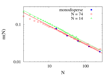
Figure 16: Average RBO as function of strand length $N$ in cross-linked networks. The lines are fits with $N^{-1/2}$.

This observation is used to compute the distribution of the RBOs in randomly crosslinked networks. The contribution of a particular active strand length $N$ is computed according to equation (31) and weighted by the $w_{N,ac}$ of the $N$-mer in the sample. The number fraction $n_{N}$ of strand lengths can be approximated by $n_{N}\approx\exp\left(-N/N_{n}\right)$ [27, 46], whereby the number average strand length $N_{n}$ is computed from the number density of crosslinks. Accordingly, the weight fraction of active strands of $N$ monomers is approximately (assuming no significant difference in the distributions of active and inactive strands) $w_{N,ac}\approx Nn_{N}/\sum_{N}Nn_{N}$. The distribution function of RBOs is then approximated by

$$P_{c}(m)\mbox{d}m\approx\sum_{N=1}^{\infty}w_{N,ac}P(m,N)\mbox{d}m.$$ (32)

The numerical solution to this equation is computed using the average virtual chain lengths $n=3.6$ and $5.3$, which were determined from the cross-link fluctuations in the networks (after normalizing by $f/(f-1)$ to account for the definition of the virtual chains). Furthermore, the same $z$ as for the corresponding end-linked samples with $N=64$ was used for comparison.

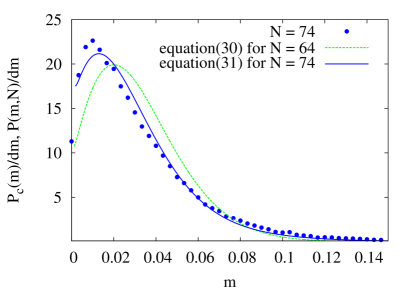
Figure 17: The distribution of RBOs of cross-linked networks compared with the predictions for end-linked (dashed line) and crosslinked (continuous line) networks.

The data of the cross-linked sample $N=74$ is shown in Figure 17 and compared with a fit of equation (32) using a variable $\gamma$ to compute of $P(m)$. The agreement between simulation data and equation (32) is good and points towards a slightly reduced $\gamma\approx 0.33$ as compared to the end-linked networks. Note that the randomly crosslinked networks have been linked rather instantaneously, while the end-linking reaction was rather slow in comparison. The different $\gamma$ for these two types of networks, can be explained, therefore, by a possible stress equilibration and redistribution of monomers when connecting two tubes at their ends by end-linking. Compared to the prediction of the end-linked networks, we further observe in Figure 17 a shift of the peak position towards smaller RBO and a larger high molecular weight tail of the distribution. This is qualitatively as expected from equation (32).

7 Discussion

To relate NMR data to the structure of entangled polymer networks, the central assumption in previous literature is to treat entanglements as additional cross-links and thus, the contributions of entanglements and cross-links to the residual dipolar coupling are additive [16, 41]. Under these assumptions, the effective elastic chain length $N_{el}$ is determined by NMR and the average network strand length $N$ is calculated from the average residual dipolar coupling using

$$N_{el}^{-1}=N^{-1}+N_{e}^{-1}\simeq N_{e}^{-1}\,\,\,\,\,\,{\mbox{for}}\,\,N\gg N_{e},$$ (33)

whereby $N_{e}$ denotes the entanglement length.

In the present work, it was shown that this approach is not consonant with slip-link or slip tube models of entangled networks, see Ref [2]. In conclusion, we cannot consider entangled chains being glued to each other like cross-linked chains. Instead, the strands fluctuate along a confining tube-like region in space leading to an RBO $m\propto N^{-1/2}$. This has important consequences for the interpretation of experimental data and for the theory of rubber elasticity.

First, the prediction of decreasing RBO $m\sim N^{-1/2}$ is not in contrast with the stress optical rule [6]: NMR measures the time average of individual bond orientations, which then becomes averaged over the entire sample. But stress is defined by the ensemble average of all instantaneous forces at a given time [6]. The former is measured for the same bonds at different positions in space, while the latter is the average over different monomers or bonds that are at the same location in space. Both quantities match coincidentally in the framework of the affine and phantom network model, since there, time and ensemble averages are fully exchangeable and stress is solely transmitted along the network bonds. Entanglements, by definition, confine the fluctuations of a chain to a given region in space depending on the particular entanglements of a given chain. Therefore, the time averages of individual chains are no longer exchangeable with the ensemble averages over all chains, which must lead to different results for the RBO (or the tensor order parameter) as compared to stress.

Second, the pronounced dependence of the RBO as function of $k$ (see Figures 10 and 13) can only be explained by introducing a mechanism that reduces the RBO towards the inner monomers of the chains. It was shown that a) monomer fluctuations increase towards the inner monomers of the chains and b) that these enhanced fluctuations can lead to a reduction of the RBO, since a larger number of uncorrelated tube sections can be visited. Such a behavior is only consonant with slip-link or slip tube models [2, 47, 48, 49], which allow the segments to slide through slip links or along the tube.

Third, with the present model it is possible to separately analyze the correlation length of the primitive path $N_{p}$ and the strength of the confining potential as expressed in the confinement length $N_{c}$. As discussed in section 4.2, a quantitative analysis of NMR data [17] suggests that the de-correlation length of the tube $N_{p}$ is about $N_{p}/N_{e}\approx 2/3$, which is in the range of theoretical estimates [2, 20, 21] that predict $N_{p}=N_{e}/2$, $4N_{e}/7$, or $4N_{e}/5$. Best agreement is found with the model of [2] that was used as a basis for the computations of the current paper.

In literature, several simulation works exist, which are closely related to the present study. Sotta et al. [50, 51, 52] use a “network” model of individual chains fixed at their ends similar to the work of Yong and Higgs [53] and analyze the effect of deformation on the RBO. The missing network structure allows dis-entanglements near the chains ends, therefore, we do not expect significant impact of the remaining entanglements for the studies using short chain lengths [51, 52, 53]. A later work [50] covers larger $N$, which are comparable to the present study. Interestingly, the author mentions that the RBO close to chain ends is generally different from that in the middle of the chains, but a detailed analysis of this point is missing.

Recently, the group of Prof. Cohen analyzed RBOs in experiments on end-linked PDMS networks and using computer simulations [54, 55, 56]. The experimental results motivated a DE-compositon of the NMR spectra into a wide and narrow one, whereby it was shown that inelastic chains contributed only partially to the narrow spectrum. This decomposition is therefore problematic since the authors cannot provide a striking physical explanation to justify the source of a second population of chains. In the present work, the simulation data are fit without introducing a second distribution of chain lengths or RBOs. In contrast, to the assumption in [54, 55, 56] it is shown, that a different RBO appears along the same chains, making the separation into two major populations obsolete. However, the results of [54, 55, 56] point out that it is essential to distinguish between active and inactive material. For instance, the simulation data of Fig 6 or Ref. [56] shows nearly identical average RBO for short and long chains in samples of 60% mol fraction of short chains. For those samples it is known that a high fraction of short chains form inactive dangling rings [46, 57] and thus, we have to expect a large fraction of chains with RBO close to zero. In consequence, in reference [56] the average segmental orientation becomes a function of composition and the average RBO of long chains eventually becomes larger as for short chains.

The determination of the entanglement length is one of the key questions of recent computational studies on entangled polymers, see Ref. [8] for a review. The methods discussed in Ref [8] either require modifying the samples for analysis (“primitive path analysis”) or to use a static analysis of conformations. For a most direct comparison of our work with previous data it is preferable to compare with dynamic data of unmodified samples. For this comparison, it is important to recognize that tube length fluctuations (TLF) are largely suppressed in for entangled active network stands, since the chain ends are tied to other active chains. But inactive network chains release here a significant amount of constraints influencing time averaged data. In the long time limit, this inactive material effectively serves as a $\theta-$solvent for the active chains dilating the tube to an apparent $N_{p}=N_{p}(1)\phi_{ac}^{2/3}$ with respect to an $N_{p}(1)$ as determined in a perfect network. Note that for this estimate we assume that the line density of entangled strands is homogeneously reduced by the weight fraction of active polymer $\phi_{\mbox{ac}}$. We further have to point out that all inactive material can be considered to be relaxed during the time period of the analysis for $N\leq 128$, see also section 10. For network $N=256$, however, a separate analysis of the RBOs of dangling chains revealed that about 25% of the dangling material is still not fully relaxed by the end of the simulation run. Therefore, the $\phi_{\mbox{ac}}$ in table 1 was estimated with respect to the fully relaxed inactive material.

In contrast to networks, constraint release is typically considered as a less important correction for mono-disperse melts while a dominating correction is attributed to TLF [4, 6]. For instance, Kreer et al. [29] or Paul et al. [39, 58] investigate entangled melts using the simulation method of the present work at the same lattice occupation of $\phi=0.5$. In ref [29], the relaxation times of melts with $N\leq 512$ are reported. It is estimated that $N_{e}\approx 38$ based upon the ratio of reptation times without considering TLF. Recall the discussion at the introduction and the fact that the reptation times were determined by an analysis based upon diffusion instead of stress relaxation. Therefore, we expect that the results of ref [29] are more related to the entanglement spacing and thus $N_{p}$ instead of $N_{e}$. The samples $N_{1}=512$ and $N_{2}=128$ of ref [29] are clearly entangled. The effect of TLF can be estimated by equating the reported ratio for the relaxation times using the Doi-Edwards correction for TLF for which we use[59] $N_{p}$ instead of $N_{e}$ as variable:

$$\frac{\tau_{rep}(N_{1})}{\tau_{rep}(N_{2})}\approx\frac{N_{1}^{3}[1-\mu\sqrt{N_{p}/N_{1}}]^{2}}{N_{2}^{3}[1-\mu\sqrt{N_{p}/N_{2}}]^{2}}.$$ (34)

Solving for $N_{p}$ using the data of ref [29] leads to $N_{p}\approx 10\pm 1$, whereby the error indicates different results obtained by considering either end-to-end vector relaxation time $\tau_{ee}$ or the relaxation for the longest mode $\tau_{1}$ while using either $\mu\approx 1$ or a more accurate estimate for $\mu$ from Figure 9.21 of [4]. This result is in excellent agreement with the persistence length of the primitive path $N_{p}$ as determined in the present work, since the extrapolated data for networks with out defects yields $N_{p}(\phi_{ac}=1)\approx 12$. In fact, following the discussion in section 4.2 we have to conclude that the diffusion data of long entangled chains must be related to $N_{p}$ instead of $N_{e}$. Note that a similar shift to $N_{p}=16\pm 5$ for the original estimate of $30\pm 15$ is obtained for Ref. [39, 58] when reanalyzing the delay of

$$\tau_{rep}/\tau_{Rouse}\approx N[1-\mu\sqrt{N_{p}/N}]^{2}/N_{p}\approx 6.67.$$ (35)

Therefore, the data in refs [29, 39, 58] fully supports our analysis about monomer fluctuations. But the results for polymer dynamics may be reinterpreted based upon $N_{p}$ instead of $N_{e}$, if the model and the analysis of the present work is confirmed by other studies.

In previous studies on melts of cyclic polymers [61, 62] using the BFM at $\phi=0.5$, an anti-correlation peak was found in the correlation function of bonds with a separation distance 11 bonds along the ring. This observation could not be understood since previous studies estimate $N_{e}\approx 30$ and assume that a de-correlation of the tube is only possible at $N_{e}$. The data of the present work, however, finds $N_{p}\approx 12$ for ideal networks. The same result may apply to melts of long rings without further corrections due to the absence of chain ends. If this agreement is confirmed by the data of different simulation models or for simulations of chains with a different stiffness, the analysis of the bond correlations in melts of long rings could be used for quick determination of the de-correlation length of the confining tube.

One of the reviewers of this work wondered why a “strangulation” of the network chains for $N\rightarrow 1$ is not observed. The strangulation regime was originally discussed [63] for unattached chains that diffuse through a network, whereby the mesh size of the network becomes smaller than the entanglement length. For the four-functional neworks of the present study, there is an average of $n\approx 8$ strands needed to form a cyclic structure inside the network [64]. The cyclic structures lead to a confinement that can be described by a virtual chain of length $nN/2$. The non-entangled elasticity of the network, on the other hand, is described by a chain of $2N$ segments (for ideal $4$-functional network) that is grafted at both ends [2]. Thus, the maximum fluctuations of inner chain monomers are described by virtual chains of roughly $N<nN/2$ segments. Since network elasticity leads to a stronger confinement, the network strands of the present study do not strangulate themselfes when crossing over to the non-entangled regime. However, the effect of strangulation can contribute to a measurable enlargement of the residual bond orientation for $N<N_{e}$, since both strangulation and elasticity have the same dependence on $N$.

In conclusion, we find supporting simulations and experimental data for the presented model for the RBO in networks. The data can only be explained by assuming a chain slippage along a confining tube or through slip links. Therefore, the results are in agreement with slip link or slip tube models [2] for networks and disagree with network models that do not explicitly allow a fluctuation of the monomers along a confining tube.

8 Summary

In this work we presented theoretical models and data for average RBO and the distribution of RBOs for entangled model networks of a) mono-disperse or b) poly-disperse weight distribution between the crosslinks, c) non-entangled “phantom” model networks and d) non-entangled “crossing” model networks with excluded volume interactions.

It is found that the phantom model correctly describes monomer fluctuations in networks without excluded volume and entanglements. Monomer fluctuations in networks with excluded volume but no entanglements can be described, if the phantom model is corrected by the effect of the incompletely screened excluded volume. This leads to larger monomer fluctuations and conversely, a weaker force that is necessary to stretch a network of excluded volume chains as compared to the phantom prediction. This result is used as a correction for the analysis of the RBOs of entangled networks.

For the analysis of entangled samples, it is distinguished between tube confinement, expressed by a confinement length $N_{c}$, and reorientation of the tube, expressed by a tube de-correlation length $N_{p}$. $N_{p}$ can be determined from monomer fluctuations of active chains attached to network junctions that are attached to a defined number of active strands. The confinement length $N_{c}$ enters in the model by the analogy between tension blobs of a stretched chain and the stretching of the chains along the primitive path. Both $N_{p}$ and $N_{c}$ contribute differently to the RBO and thus, allow a separate analysis using the model of the present work. For the BFM we find $N_{p}\approx 12$ at $\phi=0.5$ and large $N$ when extrapolating to ideal networks without defects. Previous simulation data on the dynamics of linear chains [39, 58, 29] and cyclic polymers in melts [61, 62] lead to a similar conclusion after the data on dynamics is corrected for tube length fluctuations.

The RBO in phantom networks is well predicted by the phantom model after considering the boundary conditions and the fixation of the networks in a weakly stretched state. The RBO in crossing networks with excluded volume but without entanglements shows some weak enhancement near the chain ends due to increased excluded volume interactions with attached other chains at the cross-links. The RBOs in entangled networks are quantitatively and qualitatively different from the non-entangled networks. First, the average RBO is larger, roughly by a factor $(N/N_{p})^{1/2}$. Second, there is a pronounced enhancement of RBOs near the chain ends that is caused by the reduced fluctuations of the monomers near the crosslinks. The same scaling of the RBO $\sim(NN_{p})^{-1/2}$ is observed in all entangled networks of the present study and it is confirmed by experimental data [17]. A quantitative analysis of the RBO of this experimental study suggests that the tube de-correlates at a degree of polymerization $N_{p}$ of about $2/3$ of $N_{e}$. This is in good quantitative agreement with the slip tube model [2] and not too far from other estimates [21, 20]. In conclusion, the $N_{p}$ as determined from the average RBO or the distribution of the RBOs is shorter than the entanglement length $N_{e}$.

The distribution function of the RBO agrees well with the gamma distribution in the case of phantom networks. For mono-disperse entangled networks we obtain a clearly different distribution function that is in good agreement with the simulation data. The same approach can be used for randomly cross-linked networks and it also fits to the data. The key result of our model, that the RBO of entangled networks is $\propto N^{-1/2}$, does not disagree with the stress optical rule, since NMR does not measure stress. Only in some particular cases, e.g. of network models without entanglements, there is an coincidental agreement between RBO and stress.

9 Acknowledgment

The authors thank the computing facilities at the ZIH and IPF Dresden for a generous grant of computing time. ML thanks J-U. Sommer, S. Nedelcu, A. Galuschko, K. Saalwächter, E.T. Samulski, M. Rubinstein and S. Panyukov for helpful discussions. Financial support by the DFG grant LA 2735/2-1 is acknowledged.

10 Appendix

10.1 Time averaging, relaxation, and comparison with experimental data

It was shown in a previous paper [32] that computing the residual bond and tensor orientations by using running averages of the bond and tensor orientations leads to an apparent decay $m\propto t^{-1}$ and $s\propto t^{-1/2}$ respectively. In particular, for completely uncorrelated bond orientations we have $m=\left(t/\Delta t\right)^{-1}$. This dependence limits the applicablilty of both averages to regimes at which the actual residual bond orienation decays not faster than the runnig averages. Auto-correlation functions as used previously [65] do not suffer from this limitation but require a larger number of conformations to analyze, since the results are numerically less stable.

The residual tensor orientation decays $\propto t^{-1/4}$ between the entanglement relaxation time $\tau_{e}$ and the Rouse relaxation time $\tau_{R}$ of the strand, $\tau_{e}<t<\tau_{R}$ [41]. The scaling of the RBO is derived in similar manner. In section 4, we assumed that only the initial tube section is correlated, while all other tube sections are not correlated. Thus, the RBO is reduced as function of time proportional to the return probability to the original tube section $\propto t^{-1/4}$. Since this is the same scaling as for the residual tensor orientation, we expect that both residual bond and tensor orientation scale in the same manner as function of time. Equilibrium is reached at the Rouse time of the virtual chain describing the fluctuations of the monomers next to the segment. Therefore, the proportionality $s_{k}\propto m_{k}$ extends from the non-entangled regime to the entangled regime. In consequence, we can apply all scaling results for the RBO to the experimental data. A quantiative analysis, however, requires to show that also the constant of proportionality is not affected by the crossover from the non-entanged to the entangled regime.

10.2 Finite size monomer fluctuations in small non-entangled networks

In this section it is discussed how the finite simulation size affects the crosslink fluctuations of the non-entangled “phantom” and “crossing” samples. The entangled samples are not touched by this effect, since the crosslink fluctuations are strongly suppressed by entanglements.

For the three phantom networks $N=16,$ 64, and 256 we obtain $n_{0}=11.94\pm 0.03$, $n_{0}=37.44\pm 0.05$, and $n_{0}=130\pm 1$ when using equation (6) and the corresponding average root mean square bond lengths of the active chains $b=2.68$, $b=2.72$, and $b=2.72$ respectively. The phantom model [4] predicts for ideal $f$-functional networks without defects

$$n_{0}=n_{N}=\frac{N}{f-2}.$$ (36)

The networks of the present study have a conversion of approximately $0.95\%$ and contain small dangling loops and short cyclic structures of a small number of chains that are less active [66, 67]. Therefore, we expect that an effective functionality $f_{e}\leq 3.8=0.95\cdot f$ determines the cross-link fluctuations, whereby $f_{e}$ is expected to converge towards $3.8$ for increasing $N$, since cyclic defects vanish for $N\rightarrow\infty$. $f_{e}$ can be estimated in an approximate manner by solving the above equation for $f$ and using the fits for $n_{0}=n_{N}$. The above data yields $f_{e}\approx 3.34$, $f_{e}\approx 3.74$ and $f_{e}\approx 3.97$ respectively when considering the $N+1$ segments between the junctions.

A detailed analysis of the network structure on the other hand reveals that the weight average active functionality of the junctions is $f_{a}\approx 3.38$, $f_{a}\approx 3.47$ and $f_{a}\approx 3.54$ respectively. While the result for $N=16$ is in good agreement with the fluctuation analysis, there is a strikingly increasing discrepancy for growing $N$ that is clearly beyond the error of the data as it is observable in Figure 5.

We argue that the reason for the discrepancy between both data sets is due to two finite size effects. Obviously, subtracting the center of mass motion leads in small samples to a weak correlation of cross-link fluctuations (and the material attached to the cross-link) and sample diffusion and therefore, to the measurement of increasingly smaller monomer fluctuations with decreasing number of chains. But, the more pronounced finite size effect originates from having a small network spanned by periodic boundary conditions: For the networks $N=256$, the size distribution of the cyclic structures is already dominated by cycles that are closed through the periodic boundary condition, see [68] for a more detailed discussion. This leads to an increased coupling of the fluctuations of a cross-link with its own periodic image. The magnitude of this effect can be estimated by truncating the recursive computation of monomer fluctuations at a finite number of generations of chains roughly equal to half the length of an average “periodic” network cycle recalling the derivation of the phantom model (cf. section 7.2.2 of [4]). The generation $g$ at which the total number of cross-links $M/2$ in the structure becomes comparable to the number of junctions in a tree of average functionality $f_{a}$ becomes the key quantity for this estimate. It is computed numerically by solving

$$1+\sum_{g=1}f_{a}(f_{a}-1)^{g-1}\approx M/2$$ (37)

for $g$. The solution of this equation leads to a rather small $g\approx 5$ for $M=512$ and $f_{a}\approx 3.54$. Therefore, this effect leads to an overestimation of $f_{e}$ of roughly 10% for $N=256$, while this overestimation reduces to about 1% for $N=16$. This qualitative change in the discrepancy between the numerical data for $f_{e}$ and $f_{a}$ is well reflected by the above data and contributes significantly to the shift of the RBO in Figure 7.

Table of Contents Graphic

Monomer Fluctuations and the Distribution of Residual Bond Orientations in Polymer Networks

Michael Lang

References

- [1] M. Lang, J.-U. Sommer, PRL 104, 177801 (2010).
- [2] M. Rubinstein, S. Panyukov, Macromolecules 35, 6670 (2002).
- [3] M. Rubinstein, J.Pol.Sci.B 48, 2548 (2010).
- [4] M. Rubinstein, R. Colby, Polymer Physics, Oxford University Press, New York (2003).
- [5] S. F. Edwards, Proc.Phys.Soc. (London) 92, 9 (1967).
- [6] M. Doi, S.F. Edwards, The Theory of Polymer Dynamics, Oxford University Press, New York (1986).
- [7] H. Watanabe, J.Polym.Sci. 24, 1253 (1999).
- [8] S. Shanbhag, M. Kröger, Macromolecules 40, 2897 (2007).
- [9] W. Bisbee, J. Qin, S. T. Milner, Macromolecules 44, 8972 (2011).
- [10] R. N. Khaliullin, J. D. Schieber, Macromolecules 42, 7504 (2009).
- [11] A. E. Likhtman, Viscoelasticity and Molecular Rheology. In Comprehensive Polymer Science, 2nd ed.; Elsevier, Amsterdam (2011).
- [12] One of the reviewers pointed out that the “vector” or “tensor order parameters” are indeed no true order parameters as used in statistical physics. Therefore, “residual bond orientation” or “residual tensor orientation” is used in the present work as replacement.
- [13] K. Saalwächter, Prog. NMR Spectr. 51, 1 (2007).
- [14] K. Saalwächter, P. Ziegler, O. Spyckerelle, B. Haidar, A. Vidal, J.-U. Sommer, J. Chem. Phys. 199, 3468 (2003).
- [15] K. Saalwächter, B. Herrero, M.A. Lopez-Manchado, Macromolecules 38, 9650 (2005).
- [16] P. Sotta, C. Fülber, D.E. Demco, B. Blümich, H. W. Spiess, Macromolecules 29, 6222 (1996).
- [17] P.T. Callaghan, E.T. Samulski, Macromolecules 33, 3795 (2000).
- [18] M. Knörgen, H. Menge, G. Hempel, H. Schneider, M. E. Ries, Polymer 43, 4091 (2002).
- [19] P. G. De Gennes, J. Chem. Phys. 55, 572 (1971).
- [20] R. G. Larson, T. Sridhar, L. G. Leal, G. H. McKinley, A. E. Likhtman, T. C. B. McLeish, J. Rheol, 47, 809 (2003).
- [21] R. Everaers, Phys. Rev. E 86, 022801 (2012).
- [22] E. Helfand, D.S. Pearson, J. Chem. Phys. 79 2054 (1983).
- [23] M. Rubinstein, E. Helfand, J.Chem.Phys. 79, 2054 (1985).
- [24] Consider an ideal chain that is fixed in space at both ends and connect one end of a second ideal chain to an arbitrary monomer of the first chain. The other end of this second chain is fixed at an arbitrary position in space that allows the second chain to maintain Gaussian statistics. If the fixed end of the second chain is not located on the straight line connecting both ends of the first chain, then, the time averaged conformation of the original chain is no longer a straight line connecting both ends. Since the time average conformation is no longer a straight line, the tension along the chain (as measured by the contour length of the time average conformation) wass increased by the linking both chains together.
- [25] M. Lang, M. Hoffmann, R. Dockhorn, M. Werner, J.-U. Sommer, JChemPhys 139, 164903 (2013).
- [26] I. Carmesin, K. Kremer, Macromolecules 21, 2819 (1988).
- [27] M. Lang, D. Göritz, S. Kreitmeier, Macromolecules 38, 2515 (2005).
- [28] M. Lang D. Göritz, S. Kreitmeier, Macromolecules 36, 4646 (2003).
- [29] T. Kreer, J. Baschnagel, M. Müller, K. Binder, Macromolecules 34, 1105 (2001).
- [30] W. Michalke, M. Lang, S. Kreitmeier, D. Göritz, JChemPhys. 117, 6300 (2002).
- [31] A. N. Semenov, A. Johner, Eur.Phys.J.E 12, 469 (2003).
- [32] J.-U. Sommer, K. Saalwächter, Eur.Phys.J. E 18, 167 (2005).
- [33] J.-P. Cohen Addad, Prog. NMR Spectrosc. 20, 1 (1993).
- [34] J.-U. Sommer, W. Chasse, J. L. Valentin, K. Saalwächter, Phys.Rev.E 78, 051803 (2008).
- [35] H. M. James, J. Chem. Phys. 15, 651 (1947).
- [36] H. M. James, E. Guth, J. Chem. Phys. 11, 455 (1948).
- [37] i.e. an ideal perfectly branching network without finite cyclic structures at full conversion.
- [38] J. P. Wittmer, P. Beckrich, H. Meyer, A. Cavallo, A. Johner, J. Baschnagel, Phys. Rev. E 76, 011803 (2007).
- [39] W. Paul, K. Binder, D. W. Heermann, K. Kremer, J. Phys. II 1, 37 (1991).
- [40] I. S. Gradshteyn, I.M. Ryzhik, Table of Integrals, Series, and Products, 5th Ed., Academic Press Boston (1994).
- [41] R. C. Ball, P.T. Callaghan, E.T. Samulski, J. Chem. Phys. 106, 7352-7361 (1997).
- [42] W. Gronski, D. Emeis, A. Brüderlin, M. M. Jacobi, R. Stadler, C.D. Eisenbach, Brit.Polym.J 17, 103 (1985).
- [43] W. Gronski, R. Stadler. M.M. Jacobi, Macromolecules 17, 741 (1984).
- [44] M. Doi, N.Y. Kuzuu, J.Pol.Sci Pol.Lett 18, 775 (1980).
- [45] Note that the contraction is assymmetric and thus, does not preserve the expectation value of the average RBO. This leads to a shift of the average RBO of about 5% for the RBOs of the present study which is corrected numerically for comparison with the simulation data.
- [46] J.-U. Sommer, S. Lay, Macromolecules 35, 9832 (2002).
- [47] S. F. Edwards, T. A. Vilgis, Rep. Prog. Phys. 51, 243 (1988).
- [48] R. C. Ball, M. Doi, S. F. Edwards, M. Warner, Polymer 22, 1010, (1981).
- [49] S. F. Edwards, T. A. Vilgis, Polymer 27, 483 (1986).
- [50] P. Sotta, Macromolecules 31, 8417 (1998).
- [51] P. Sotta, P.G. Higgs, M. Depner, B. Deloche, Macromolecules 28, 7208 (1995).
- [52] M. Depner, B. Deloche, P. Sotta, Macromolecules 27, 5192 (1994).
- [53] C. W. Yong, P. G. Higgs, Macromolecules 32, 5062-5071 (1999).
- [54] G. D. Genesky, T. M. Duncan, C. Cohen, Macromolecules 42, 8882 (2009).
- [55] B. M. Aguilera-Mercado, C. Cohen, F. A. Escobedo, Macromolecules 42, 8889 (2009).
- [56] B. M. Aguilera-Mercado, G. D. Genesky, T. M. Duncan, C. Cohen, F. A. Escobedo, Macromolecules 43, 7173 (2010).
- [57] W. Michalke, M. Lang, A. Buchner, S. Kreitmeier, D. Göritz, CompTheoPolSci 11 459 (2001).
- [58] W. Paul, K. Binder, D. W. Heermann, K. Kremer, J. Chem. Phys. 95, 7726 (1991).
- [59] The theory for equation (34) was developed for by assuming that any correlated section of the primitive path contributes to the modulus. It was further estimated that for a continuous Rouse chain model in ref [60]. Note that a different numerical model might lead to a different numerical result for . For instance, in Fig. 9.21 of Rubinstein and Colby, the data of a repton model simulation is well approximated by . The basic length step of this simulation is equivalent to of my work. Since both repton model and my simulations consist of non-continuous Rouse chains, I expect that and as basic step length is more suitable to obtain a quantitative estimate for the effect of tube length fluctuations.
- [60] M. Doi, J.Pol.Sci.Pol.Phys. 21, 667 (1983).
- [61] M. Müller, J. P. Wittmer, M. E. Cates, Phys. Rev E 61, 4078 (2000).
- [62] M. Lang, Macromolecules 46, 1158, (2013).
- [63] De Gennes, Macromolecules 19, 1249 (1986).
- [64] M. Lang, S. Kreitmeier, D. Göritz, Rubber Chemistry and Technology 80, 873 (2008).
- [65] Z. Wang, A. E. Likhtman, R. G. Larson, Macromolecules 45, 3557 (2012).
- [66] M. Lang, K. Schwenke, J.-U. Sommer, Macromolecules 45, 4886 (2012).
- [67] P. Flory, Proceedings of the Royal Society London A 351, 351 (1976).
- [68] M. Lang, “Bildung und Struktur in Polymeren Netzwerken”, Dissertation, University of Regensburg (2004).