Linearly-constrained nonsmooth optimization for training autoencoders

Abstract

A regularized minimization model with $l_{1}$-norm penalty (RP) is introduced for training the autoencoders that belong to a class of two-layer neural networks. We show that the RP can act as an exact penalty model which shares the same global minimizers, local minimizers, and d(irectional)-stationary points with the original regularized model under mild conditions. We construct a bounded box region that contains at least one global minimizer of the RP, and propose a linearly constrained regularized minimization model with $l_{1}$-norm penalty (LRP) for training autoencoders. A smoothing proximal gradient algorithm is designed to solve the LRP. Convergence of the algorithm to a generalized d-stationary point of the RP and LRP is delivered. Comprehensive numerical experiments convincingly illustrate the efficiency as well as the robustness of the proposed algorithm.

90C26, 90C30

1 Introduction

A deep neural network (DNN) [28] aims to solve a finite-sum minimization problem

(1) $$\min_{{W_{\ell},b_{\ell},\ell=1\ldots,L}}\frac{1}{N}\sum_{n=1}^{N}\psi_{n}({\varphi_{n,L}}(W_{1},\ldots,W_{L},b_{1},\ldots,b_{L})).$$

Here $\varphi_{n,L}(W_{1},\ldots,W_{L},b_{1},\ldots,b_{L})=\sigma_{L}(W_{L}\sigma_{L-1}(\cdots\sigma_{1}(W_{1}x_{n}+b_{1})+\cdots)+b_{L})$ denotes the outputs of the $L$-th hidden layer, and $\psi_{n}$ denotes the loss function measuring the output $\varphi_{n,L}(W_{1},\ldots,W_{L},b_{1},\ldots,b_{L})$ and its corresponding true output for $n=1,\ldots,N$, where $\{x_{n}\}_{n=1}^{N}$ is the data set, $W_{\ell}\in\mathbb{R}^{N_{\ell}\times N_{\ell-1}}$, $b_{\ell}\in\mathbb{R}^{N_{\ell}}$, $\sigma_{\ell}:\mathbb{R}^{N_{\ell}}\mapsto\mathbb{R}^{N_{\ell}}$ ($\ell=1,\ldots,L$) are the weight matrices, the bias vectors and the activation functions, respectively.

A broad class of methods, based on stochastic gradient descent (SGD), are proposed to solve (1), such as the vanilla SGD [9], the Adadelta [38], and the Adam [20]. In SGD methods, the gradient of the objective function is calculated by the chain rule, which is applicable to smooth activation functions, such as sigmoid, hyperbolic, and softmax functions [14]. However if a nonsmooth activation function is used, such as the rectified linear unit (ReLU) or the leaky ReLU [27], the subgradient of the objective function in (1) is difficult to calculate. At least the chain rule is no longer useful (see [8, Theorem 10.6]). As shown by recent studies, such nonsmooth activation functions have some advantages over the aforementioned smooth ones, as they can pursue the sparsity of the network [13]. The readers may refer to Glorot et al. [13] and Jarrett et al. [18] for the numerical comparisons between the DNN with smooth activation functions and those with nonsmooth ones. Due to excellent numerical behavior, the ReLU activation function has been widely used since 2010 [1, 11, 30, 33, 37]. In practice, the SGD based approaches are still used to tackle the problem with nonsmooth activation functions. The exactness in calculating the subgradient of a nonsmooth function is usually neglected in SGD methods. Gradients in a neighborhood are often used to approximate the one at a nonsmooth point. Certainly, such approximation may cause theoretical and numerical troubles in some cases. Hence, it is worthwhile to develop algorithms for solving problem (1) with nonsmooth activation functions and deal with the nonsmoothness appropriately.

In [5], Carreira-Perpiñán and Wang reformulate problem (1) as the following constrained optimization problem with $u_{n,0}=x_{n}$ for all $n=1,2,\ldots,N$,

(2) $$\min_{{W_{\ell},b_{\ell},u_{n,\ell}}\atop{\ell=1,\ldots,L,n=1,\ldots,N}} \,\frac{1}{N}\sum_{n=1}^{N}\psi_{n}(u_{n,L})$$

$${\rm s.t.} \,u_{n,\ell}=\sigma_{\ell}(W_{\ell}u_{n,\ell-1}+b_{\ell}),\quad n=1,\ldots,N,\,\ell=1,\ldots,L,$$

and propose a method of auxiliary coordinates to solve (2). Moreover, an alternating direction method of multipliers (ADMM) [34] and a block coordinate descent method (BCD) [22] are proposed to solve the constrained model and its $l_{2}$-norm penalty problem, respectively. However, these methods are less efficient than SGD based approaches, and lack of theoretical guarantee (see [39]).

More recently, Cui et al. [10] use an $l_{1}$-norm penalty method to replace the constraints in (2) by adding $\sum^{N}_{n=1}\sum^{L}_{\ell=1}\|u_{n,\ell}-\sigma_{\ell}(W_{\ell}u_{n,\ell-1}+b_{\ell})\|_{1}$ in the objective function. They provide an exact penalty analysis and establish the convergence of the sequence generated by their proposed algorithm to a directional stationary point, which will be defined in (2.1). To the best of our knowledge, this is the first mathematically rigorous method for training deep neural networks with nonsmooth activation functions. However, some assumptions imposed in their theoretical analysis are restrictive for some applications. For instance, the ReLU does not satisfies the assumptions on activation functions in [10, Corollary 2.2]. Moreover, the boundedness assumption on the sequences of iterates imposed for convergence analysis is not natural since the solution set of (2) is unbounded. For example, suppose that $\{\bar{u}_{n,\ell},\bar{W}_{\ell},\bar{b}_{\ell}\}_{\ell=1,n=1}^{L,N}$ is a global minimizer of model (2), it is easy to verify that $\{{\hat{u}_{n,\ell},\hat{W}_{\ell},\hat{b}_{\ell}}\}_{\ell=1,n=1}^{L,N}$ is also a global minimizer, where

$$\hat{u}_{n,1}=t\,\bar{u}_{n,1},\hat{W}_{1}=t\bar{W}_{1},\hat{b}_{1}=t\bar{b}_{1},\hat{u}_{n,2}=\bar{u}_{n,2},\hat{W}_{2}=\frac{1}{t}\bar{W}_{2},\hat{b}_{2}=\frac{1}{t}\bar{b}_{2},$$

$$\hat{u}_{n,\ell}=\bar{u}_{n,\ell},\hat{W}_{\ell}=\bar{W}_{\ell},\hat{b}_{\ell}=\bar{b}_{\ell},\quad\mbox{for\,}\,\,n=1,\ldots,N,\ell=3,...,L$$

for any $t>0$. Let $t$ tend to infinity, if $\bar{W}_{1}\neq 0$ or $\bar{b}_{1}\neq 0$, then the norm of $\{{\hat{u}_{n,\ell},\hat{W}_{\ell},\hat{b}_{\ell}}\}_{\ell=1,n=1}^{L,N}$ tends to infinity.

To overcome the unboundness of the solution set of (2), in this paper we consider the regularized model of problem (2) in [5], which adds the regularization term $\|W_{\ell}\|_{F}^{2}$ in the objective function. Motivated by the ideas of the exact $l_{1}$-norm penalty and directional stationarity in [10], we design a deterministic algorithm for training the autoencoder, a special two-layer network, using ReLU, with guaranteed convergence, and achieve competitive performances comparing with the SGD based approaches in solving large-scale problems. Our proposed model can be generalized to problem (2) with certain regularizing term (see (33)–(35) in the conclusion part.). In fact, the number of layers does not affect the validity of our theoretical analysis on the model. The reason we focus on the autoencoder in this paper is that a large number of layers does increase lots of tedious notations as well as rapidly increasing number of variables which requires further development on the algorithm to maintain the comparability with existing approaches. Such development is out of the main scope of this paper.

1.1 Regularized Autoencoders

Training an autoencoder using ReLU as the activation function can be formulated as the following nonsmooth nonconvex finite-sum minimization problem.

(3) $$\min_{W,b}\frac{1}{N}\sum_{n=1}^{N}\|\sigma(W^{\top}\sigma(Wx_{n}+b_{1})+b_{2})-x_{n}\|_{2}^{2},$$

where $\{x_{n}\in\mathbb{R}^{N_{0}}\}_{n=1}^{N}$ is the given data, $W\in\mathbb{R}^{N_{1}\times N_{0}}$ is the weight matrix, $b_{1}\in\mathbb{R}^{N_{1}}$ and $b_{2}\in\mathbb{R}^{N_{0}}$ are the bias vectors. For convenience, we use $X=(x_{1},x_{2},\ldots,x_{N})\in\mathbb{R}^{N_{0}\times N}$ to denote the data matrix, and denote $b={(b_{1}^{\top},b_{2}^{\top})^{\top}}\in\mathbb{R}^{N_{1}+N_{0}}$ as the combination of two bias vectors. Here, we select $W^{\top}$ as the weight matrix of the second layer, which is the transpose of that of the first layer. The consequent model (3) is called the autoencoder with tied weight which has been widely used in practice (see in [14, 16]). However, there exists autoencoder without tied weight, namely, the weight matrices of the two layers take $W_{1}$ and $W_{2}$, respectively (see in [31]). Nevertheless, Li and Nguyen [26] have shown that by using the tied weight, the training speed is increasing and the numerical performance is comparable than that without tied weight. Then, it becomes uncommon to consider the general case. On the other hand, our new model, algorithm and theorectical analysis can be generalized to the autoencoder without tied weight easily.

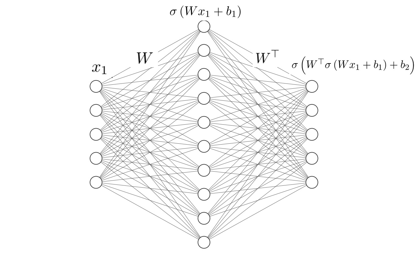
(a)

Figure 1: Illustration of the network of an autoencoder

In this paper, we focus on the ReLU, i.e. $\sigma(y)=y_{+}:=\max\{0,y\}$. An autoencoder aims to learn a prediction function $\sigma(W^{\top}\sigma(Wx_{n}+b_{1})+b_{2})$ for the given data $\{x_{n}\in\mathbb{R}^{N_{0}}\}_{n=1}^{N}$ without any label, since $\{x_{n}\}_{n=1}^{N}$ is also regarded as the true value of the output layer. Hence, the autoencoder is classified as an unsupervised learning tool. In recent years, autoencoders have been widely used in denoising, dimensionality reduction, and feature learning (e.g., [3, 23, 36]). Besides, autoencoders can be used as a preprocessing tool before training a DNN (e.g., [16, 32]).

In practice, directly solving (3) may lead to overfitting or ill-condition. To conquer these issues, the authors of [14] introduce two regularization terms to guarantee the model’s robustness. The first class of regularizers is the $l_{F}$-norm term $\|W\|_{F}^{2}$, called weight decay, which can effectively avoid the overfitting phenomenon [21]. The second class is the $l_{1}$-norm that can pursue the sparsity [14, 31]. In this paper, we use the $l_{F}$-norm for the weight matrix and the $l_{1}$-norm for the auxiliary vectors. To present our optimization model in $R^{N_{2}}$ with $N_{2}=N_{0}N_{1}+N_{1}+N_{0}+N_{1}N$, we introduce a vector variable

(4) $$z=(\mathrm{vec}(W)^{\top},b^{\top},\mathrm{vec}(V)^{\top})^{\top}\in\mathbb{R}^{N_{2}},$$

where $V=(v_{1},v_{2},\ldots,v_{N})\in\mathbb{R}^{N_{1}\times N}$ is an auxiliary variable with $v_{n}=(Wx_{n}+b_{1})_{+}$ for all $n=1,\ldots,N$, and $\mathrm{vec}(Y)\in\mathbb{R}^{lm}$ denotes the columnwise vectorization of the matrix $Y\in\mathbb{R}^{l\times m}$. Let

$$\mathcal{F}(z)=\frac{1}{N}\sum_{n=1}^{N}\|(W^{\top}v_{n}+b_{2})_{+}-x_{n}\|_{2}^{2}\quad{\rm and}\quad\mathcal{R}(z)=\lambda_{1}\sum_{n=1}^{N}e^{\top}v_{n}+\lambda_{2}\|W\|_{F}^{2}$$

denote the fidelity term and regularization term, respectively, where $e=(1,\ldots,1)^{\top}\in\mathbb{R}^{N_{1}}$ and $\lambda_{1},\lambda_{2}>0$. We consider the following Regularized (R) minimization model for the autoencoders

(R) $$\min_{z} \mathcal{F}(z)+\mathcal{R}(z)$$

s.t. $$z\in\Omega_{1}:=\left\{z:v_{n}=(Wx_{n}+b_{1})_{+},\,n=1,\ldots,N\right\}.$$

We would like to mention that the equivalent form of problem (R), namely (3) with regularizer $\mathcal{R}$, has been widely used in autoencoders (see in [14, 36]).

1.2 Our Focuses and Motivation

The feasible set $\Omega_{1}$ of problem (R) is nonconvex and the standard constraint qualifications may fail due to the nonsmooth equality constraints in (R). Hence, we introduce the following Regularized minimization model with $l_{1}$-norm Penalty (RP) for the autoencoders.

(RP) $$\min_{z} \mathcal{O}(z):=\mathcal{F}(z)+\mathcal{R}(z)+\mathcal{P}(z)$$

s.t. $$z\in\Omega_{2}:=\left\{z:v_{n}\geq(Wx_{n}+b_{1})_{+},\,n=1,\ldots,N\right\},$$

where $\mathcal{P}(z):=\beta\sum_{n=1}^{N}e^{\top}\left(v_{n}-(Wx_{n}+b_{1})_{+}\right)$ is the penalty term.

Compared with the $l_{1}$-norm penalty term $\sum_{n=1}^{N}\left\|v_{n}-(Wx_{n}+b_{1})_{+}\right\|_{1}$ proposed in [10], the subdifferential of $\mathcal{P}(z)$ enjoys an explicit expression. In addition, the feasible set $\Omega_{2}$ of (RP) is convex and the slater-type constraints qualification holds [8, Section 6.3, Proposition 6.3.1]. However, the solution set of (RP) may be unbounded as that of the model in [10]. To overcome the unboundness and ensure the sequence generated by the algorithm is bounded, we introduce a convex set

$$\Omega_{3}:=\left\{z:\|b\|_{\infty}\leq\alpha\right\},$$

where

(5) $$\alpha=\max\left\{\frac{\theta}{\lambda_{1}}+\sqrt{\frac{N_{1}N_{0}\theta}{\lambda_{2}}}\|X\|_{1},\frac{\theta\sqrt{N_{1}N_{0}\theta}}{\lambda_{1}\sqrt{\lambda_{2}}}+\sqrt{N\theta}+\|X\|_{1}\right\},\,\,\theta>\frac{1}{N}\|X\|_{F}^{2}.$$

We will show that (RP) has a global solution in $\Omega_{3}$. Hence, it suffices to solve (RP) restricted to $\Omega_{3}$. Note that $v_{n}\geq(Wx_{n}+b_{1})_{+}$ can be represented by $v_{n}\geq Wx_{n}+b_{1}$ and $v_{n}\geq 0$. Let $\nu=2(NN_{1}+N_{0}+N_{1})$,

$$A=\left[\begin{array}[]{ccc}\makebox[0.0pt][l]{$\smash{\overbrace{\phantom{\begin{matrix}X^{\top}\otimes I_{N_{1}}\end{matrix}}}^{\text{$W:N_{0}N_{1}$}}}$}X^{\top}\otimes I_{N_{1}}&\makebox[0.0pt][l]{$\smash{\overbrace{\phantom{\begin{matrix}e_{N}\otimes[I_{N_{1}}\,\,\,\textbf{0}]\end{matrix}}}^{\text{$b:N_{1}+N_{0}$}}}$}e_{N}\otimes[I_{N_{1}}\,\,\,\textbf{0}]&\makebox[0.0pt][l]{$\smash{\overbrace{\phantom{\begin{matrix}-I_{N_{1}N}\end{matrix}}}^{\text{$V:NN_{1}$}}}$}-I_{N_{1}N}\\ \textbf{0}&\textbf{0}&-I_{N_{1}N}\\ \textbf{0}&I_{N_{1}+N_{0}}&\textbf{0}\\ \textbf{0}&-I_{N_{1}+N_{0}}&\textbf{0}\end{array}\right]\in\mathbb{R}^{\nu\times N_{2}},\quad c=\left[\begin{array}[]{c}\textbf{0}\\ \textbf{0}\\ \alpha e_{N_{1}+N_{0}}\\ \alpha e_{N_{1}+N_{0}}\end{array}\right]\in\mathbb{R}^{\nu},$$

where $\otimes$ represents the Kronecker product, $e_{N}\in\mathbb{R}^{N}$, $e_{N_{1}+N_{0}}\in\mathbb{R}^{N_{1}+N_{0}}$ denote the vector whose elements are all one. We consider the following Linearly constrained Regularized minimization model with $l_{1}$-norm Penalty (LRP)

(LRP) $$\min_{z} \,\,\mathcal{O}(z)$$

s.t. $$\,\,z\in\mathcal{Z}:=\Omega_{2}\cap\Omega_{3}=\{z:Az\leq c\}.$$

1.3 Contribution

We propose a partial penalty model (RP) and establish the equivalence between the models (RP) and (R) regarding global minimizers, local minimizers, and directional stationary points under some mild conditions. Moreover, we show that the solution set of (LRP) is bounded and contains at least one of global minimizers of (RP), and provide conditions such that (LRP) and (RP) have the same local minimizers and directional stationary points in ${\cal Z}$.

We propose a smoothing proximal gradient algorithm for solving (LRP), whose subproblem at each iteration is a structured strongly convex quadratic program. We develop a splitting algorithm for solving the subproblem by using the special structure, which is faster than the “quadprog” [35] and the “CVX” [15]. We prove that the sequence generated by our algorithm converges to a generalized directional stationary point of (LRP) without assuming the boundness of sequences or existence of accumulation points.

The numerical experiments demonstrate that our algorithm, equipped with adaptively selected stepsize and smoothing parameters, outperforms the popular SGD methods (e.g., Adam, Adadelda, and vanilla SGD) in acquiring better and more robust solutions to a group of randomly generated data sets and one real data set for autoencoders. More specifically, compared with SGD methods, our algorithm achieves lower training error and objective function values, and obtains sparser solutions to testing problems.

1.4 Notations and Organizations

Let $\mathcal{B}_{\epsilon}(y)$ be the closed Euclidean ball in $\mathbb{R}^{m}$ centered at $y$ and radius $\epsilon$. The $m\times m$ identity matrix is denoted by $I_{m}$. Given a nonempty closed set $\Omega$ and a point $y^{*}$, we use $\textnormal{dist}(y^{*},\Omega)=\inf_{y\in\Omega}||y-y^{*}||_{2}$ to denote the distance from $y^{*}$ to $\Omega$. We use $\mathrm{co}(\Omega)$ to represent convex hull of $\Omega$.

The rest of this paper is organized as follows. In Section 2, we give theoretical results for the relationship among the three models (R), (RP) and (LRP). In Section 3, we propose a smoothing proximal gradient algorithm for solving (LRP) and present the global convergence of the algorithm. In Section 4, we illustrate the performance of our proposed algorithm through comprehensive numerical experiments. Concluding remarks are given in the last section.

2 Model Analysis

In this section, we aim to theoretically investigate the relationship among problems (R), (RP) and (LRP) for autoencoders.

2.1 Preliminaries

In this subsection, we present some preliminary definitions. Let $\mathrm{Proj}_{\Omega}(y^{*})=\arg\min\left\{\|y-y^{*}\|_{2}:y\in\Omega\right\}$ denote the orthogonal projection of a vector $y^{*}\in\mathbb{R}^{m}$ onto a convex set $\Omega\subseteq\mathbb{R}^{m}$.

The Clarke subdifferential [8, Section 1.2] of a locally Lipschitz continuous function $f:\mathbb{R}^{m}\to\mathbb{R}$ at $y^{*}$ is defined by $\partial f\left(y^{*}\right)=\operatorname{co}\left\{\lim_{y\rightarrow y^{*}}\nabla f(y):f\text{ is smooth at }y\right\}$.

We use $f^{\prime}\left(y;d\right)$ to denote the directional derivative of a directional differentiable function $f$ at $y$ along the direction $d$, i.e.,

(6) $$f^{\prime}\left(y;d\right)=\lim_{t\downarrow 0}\frac{f(y+td)-f(y)}{t}.$$

A function $f$ is said to be regular [8, Definition 2.3.4] at $\bar{y}\in\mathbb{R}^{m}$ provided that if for all $d$, the directional derivative $f^{\prime}(\bar{y};d)$ exists, and

$$f^{\prime}(\bar{y};d)=f^{\circ}(\bar{y};d),$$

where $f^{\circ}(\bar{y};d):=\limsup_{{y\rightarrow\bar{y}}\atop{t\downarrow 0}}\frac{f(y+td)-f(y)}{t}$ is the generalized directional derivative at $\bar{y}$ along the direction $d$ [8].

It is known that if $f$ is piecewise smooth and Lipschitz continuous in a neighborhood of $y$, then $f$ is semismooth and directional differentiable at $y$ [29]. The objective functions of (R), (RP) and (LRP) are locally Lipschitz and piecewise smooth. Hence they are semismooth functions and directional differentiable.

Let $\mathcal{T}_{\Omega}(\bar{y})=\{d:d=\lim_{y\in\Omega,y\rightarrow\bar{y},\tau\downarrow 0}\frac{y-\bar{y}}{\tau}\}$ be the tangent cone of a set $\Omega$ at $\bar{y}$.

Definition 2.1.

We call $\bar{z}\in\Omega_{1}$, $\bar{z}\in\Omega_{2}$, $\bar{z}\in\mathcal{Z}$ a d(irectional)-stationary point [10] of problems (R), (RP) and (LRP), respectively, if

(7) $$\mathcal{F}^{\prime}\left(\bar{z};d\right)+\nabla\mathcal{R}(\bar{z})^{\top}d\geq 0,\quad\forall d\in\mathcal{T}_{\Omega_{1}}(\bar{z}),$$

(8) $$\mathcal{O}^{\prime}\left(\bar{z};d\right)\geq 0,\quad\forall d\in\mathcal{T}_{\Omega_{2}}(\bar{z}),$$

(9) $$\mathcal{O}^{\prime}\left(\bar{z};d\right)\geq 0,\quad\forall d\in\mathcal{T}_{\mathcal{Z}}(\bar{z}).$$

We call $\bar{z}\in\Omega_{1}$, $\bar{z}\in\Omega_{2}$, $\bar{z}\in\mathcal{Z}$ a generalized d(irectional)-stationary point of problems (R), (RP) and (LRP), respectively, if (7)–(9) hold with $\mathcal{F}^{\circ}(\bar{z};d)$ and $\mathcal{O}^{\circ}(\bar{z};d)$ instead of $\mathcal{F}^{\prime}(\bar{z};d)$ and $\mathcal{O}^{\prime}(\bar{z};d)$.

We call $\bar{z}\in\mathcal{Z}$ a generalized KKT point of (LRP) if there exists a nonnegative vector $\bar{\gamma}\in\mathbb{R}^{\nu}$ such that

(10) $$0\in\partial{\cal O}(\bar{z})+A^{\top}\bar{\gamma},\,\quad\bar{\gamma}^{\top}\left(A\bar{z}-c\right)=0,\,\quad A\bar{z}-c\leq 0.$$

2.2 Global and Local Solutions

Let $\mathcal{S}^{*}$, $\mathcal{S}$ and ${\cal Z}^{*}$ be the global solution sets of (R), (RP) and (LRP), respectively. In this subsection, we prove $\mathcal{S}^{*}$, $\mathcal{S}$ and ${\cal Z}^{*}$ are not empty, and ${\cal Z}^{*}\subset\mathcal{S}=\mathcal{S}^{*}$.

We define a level set of problem (RP) using $\theta$ defined in (5) as follows

$$\Omega_{\theta}=\{z\in\Omega_{2}:\mathcal{O}(z)\leq\theta\}.$$

Obviously, $0\in\Omega_{\theta}$ since ${\cal O}(0)=\frac{1}{N}\|X\|_{F}^{2}<\theta$ and $0\in\Omega_{2}$.

Theorem 2.2.

For any $z\in\Omega_{\theta}$, the following statements hold.

(a) $\|W\|_{F}^{2}\leq\frac{\theta}{\lambda_{2}},\|V\|_{1}\leq\frac{\theta}{\lambda_{1}}$ and $\|b_{+}\|_{\infty}\leq\alpha$.

(b) $\bar{z}=\mathrm{Proj}_{\Omega_{3}}(z)\in\mathcal{Z}$ and $\mathcal{O}(\bar{z})=\mathcal{O}(z).$

Moreover, the solution set ${\cal Z}^{*}$ of (LRP) is not empty and bounded, and ${\cal Z}^{*}\subset{\cal S}$.

Proof 2.3.

(a) The first two inequalities are from $V\geq 0$, $\mathcal{O}(z)\leq\theta$, $\mathcal{F}(z)\geq 0$, $\mathcal{P}(z)\geq 0$ and $\mathcal{R}(z)\geq 0$, which imply

(11) $$\lambda_{1}\sum_{n=1}^{N}e^{\top}v_{n}\leq\theta\,\,\,{\rm and}\,\,\,\lambda_{2}\|W\|_{F}^{2}\leq\theta.$$

Now we prove $\|b_{+}\|_{\infty}\leq\alpha$. From the Cauchy inequality and (11), we have

(12) $$\sum_{j=1}^{N_{1}}\sum_{s=1}^{N_{0}}|W_{j,s}|\leq\sqrt{N_{1}N_{0}}\|W\|_{F}\leq\sqrt{\frac{N_{1}N_{0}\theta}{\lambda_{2}}}.$$

For $n=1,\ldots,N$, combining (11) with $z\in\Omega_{2}$, we obtain that

(13) $$\frac{\theta}{\lambda_{1}}\geq e^{\top}v_{n}\geq e^{\top}(Wx_{n}+b_{1})_{+}\geq(W_{j,\cdot}x_{n}+b_{1,j})_{+}\geq W_{j,\cdot}x_{n}+b_{1,j}$$

for all $j=1,\ldots,N_{1}$. On the other hand, (12) yields $\|W_{j,\cdot}\|_{\infty}\leq\sqrt{\frac{N_{1}N_{0}\theta}{\lambda_{2}}}$, which implies

(14) $$|W_{j,\cdot}x_{n}|\leq\sqrt{\frac{N_{1}N_{0}\theta}{\lambda_{2}}}\|X\|_{1}.$$

Together with (13), we can conclude that $b_{1,j}$ satisfies

(15) $$b_{1,j}\leq\frac{\theta}{\lambda_{1}}+\sqrt{\frac{N_{1}N_{0}\theta}{\lambda_{2}}}\|X\|_{1},\quad\forall j=1,\ldots,N_{1}.$$

From ${\cal F}(z)\leq\theta$, we have

(16) $$\sqrt{N\theta}\geq(W_{\cdot,j}^{\top}v_{n}+b_{2,j})_{+}-X_{j,n}\geq W_{\cdot,j}^{\top}v_{n}+b_{2,j}-X_{j,n}$$

for all $n=1,\ldots,N$ and $j=1,\ldots,N_{0}$. From $\|v_{n}\|_{1}\leq\frac{\theta}{\lambda_{1}}$ and $\|W_{\cdot,j}\|_{1}\leq\sqrt{\frac{N_{1}N_{0}\theta}{\lambda_{2}}}$, we find

(17) $$|W_{\cdot,j}^{\top}v_{n}|\leq\frac{\theta\sqrt{N_{1}N_{0}\theta}}{\lambda_{1}\sqrt{\lambda_{2}}}.$$

Together with (16), we obtain that

(18) $$b_{2,j}\leq\frac{\theta\sqrt{N_{1}N_{0}\theta}}{\lambda_{1}\sqrt{\lambda_{2}}}+\sqrt{N\theta}+\|X\|_{1},\quad\forall j=1,\ldots,N_{0}.$$

Combining (15) and (18), we finally arrive at the assertion that $\|b_{+}\|_{\infty}\leq\alpha$.

$($b$)$ Let $\bar{z}=(\mathrm{vec}(\bar{W})^{\top},\bar{b}^{\top},\mathrm{vec}(\bar{V})^{\top})^{\top}$ with $\bar{W}=W$, $\bar{V}=V$ and

(19) $$\bar{b}_{1,j_{1}}=\left\{\begin{aligned} &b_{1,j_{1}}\,\,\,\text{if }{b}_{1,j_{1}}\geq-\alpha,\\ &-\alpha\,\,\,\text{otherwise,}\end{aligned}\right.\quad\quad\bar{b}_{2,j_{2}}=\left\{\begin{aligned} &b_{2,j_{2}}\,\,\,\text{if }{b}_{2,j_{2}}\geq-\alpha,\\ &-\alpha\,\,\,\text{otherwise}\end{aligned}\right.$$

for all $j_{1}=1,\ldots,N_{1}$, $j_{2}=1,\ldots,N_{0}$. By part (a), we have $\|\bar{b}\|\leq\alpha$. Hence $\bar{z}\in\Omega_{3}.$

By (14) and (17), we have

$${b}_{1,j_{1}}+{W}_{j_{1},\cdot}x_{n}\leq\bar{b}_{1,j_{1}}+\bar{W}_{j_{1},\cdot}x_{n}\leq-\alpha+\sqrt{\frac{N_{1}N_{0}\theta}{\lambda_{2}}}\|X\|_{1}\leq 0,\,\,{\rm if}\,\,\bar{b}_{1,j_{1}}=-\alpha,$$

$${b}_{2,j_{2}}+{W}_{\cdot,j_{2}}^{\top}v_{n}\leq\bar{b}_{2,j_{2}}+\bar{W}_{\cdot,j_{2}}^{\top}\bar{v}_{n}\leq-\alpha+\frac{\theta\sqrt{N_{1}N_{0}\theta}}{\lambda_{1}\sqrt{\lambda_{2}}}\leq 0,\,\,\,\quad\quad{\rm if}\,\,\bar{b}_{2,j_{2}}=-\alpha,$$

which together with (19) implies that for all $n=1,\ldots,N$, it holds

(20) $$(\bar{W}x_{n}+\bar{b}_{1})_{+}=(Wx_{n}+b_{1})_{+}\,\,{\rm and}\,\,(\bar{W}^{\top}\bar{v}_{n}+\bar{b}_{2})_{+}=(W^{\top}v_{n}+b_{2})_{+}.$$

Combining with $\bar{W}=W$ and $\bar{V}=V$, we have $\mathcal{O}(\bar{z})=\mathcal{O}(z).$ Moreover (20), $\bar{W}=W$ and $\bar{V}=V$ yield $\bar{z}\in\Omega_{2}$. Hence by the definition of $\bar{z}$, $\bar{z}=\mathrm{Proj}_{\Omega_{3}}(z)\in\Omega_{2}\cap\Omega_{3}={\cal Z}$.

Now we prove the last statement. By parts (a) and (b), the set ${\cal Z}\cap\Omega_{\theta}$ is a bounded closed set. Hence, there exists $z^{*}\in{\cal Z}^{*}$ such that $\mathcal{O}(z^{*})=\min_{z\in\mathcal{Z}}\mathcal{O}(z)\leq\theta.$ Assume on contradiction that $z^{*}\in{\cal Z}^{*}$, but $z^{*}\not\in\mathcal{S}$. Then there exists $\widetilde{z}\in\Omega_{2}$ such that $\mathcal{O}(\widetilde{z})<\mathcal{O}(z^{*})\leq\theta$. As we have proved in $($b$)$, $\bar{z}=$Proj${}_{\Omega_{3}}(\widetilde{z})\in\mathcal{Z}$ and $\mathcal{O}(\bar{z})=\mathcal{O}(\widetilde{z}),$ which implies $\mathcal{O}(\bar{z})<\mathcal{O}(z^{*})$. This is a contradiction. Hence ${\cal Z}^{*}\subset{\cal S}$.

The following theorem shows that (RP) is an exact penalty formulation of (R) regarding global minimizers if the penalty parameter $\beta$ in ${\cal P}$ is larger than a computable number.

Theorem 2.4.

The following statements hold.

(a) The functions $\mathcal{F}$ and $\mathcal{R}$ are Lipschitz continuous over $\Omega_{\theta}$.

(b) Let $L_{\mathcal{F}}$ and $L_{\mathcal{R}}$ be Lipschitz modulus of $\mathcal{F}$ and $\mathcal{R}$ over $\Omega_{\theta}$, respectively. Suppose $\beta>L_{\mathcal{F}}$+$L_{\mathcal{R}}$. If $\bar{z}\in\Omega_{\theta}$ is a global minimizer of (R), then $\bar{z}$ is also a global minimizer of (RP).

(c) Let $\delta:=3\theta+\frac{2N\theta^{3}}{\lambda_{1}^{2}\lambda_{2}}$ and $\Omega_{\delta}=\{z\in\Omega_{2}:\mathcal{O}(z)\leq\delta\}$. Let $L_{\mathcal{F}}$ and $L_{\mathcal{R}}$ be Lipschitz modulus of $\mathcal{F}$ and $\mathcal{R}$ over $\Omega_{\delta}$ respectively. Suppose $\beta>L_{\mathcal{F}}$+$L_{\mathcal{R}}$. If $\bar{z}\in\Omega_{\theta}$ is a global minimizer of (RP), then $\bar{z}$ is also a global minimizer of (R).

Proof 2.5.

(a) From Theorem 2.2 (a), it is clear that $\mathcal{R}$ is Lipschitz continuous over $\Omega_{\theta}$. From Theorem 2.2 (a)-(b), the set ${\cal Z}\cap\Omega_{\theta}$ is bounded. Suppose that $L_{\mathcal{F}}$ is the Lipschitz constant of $\mathcal{F}$ over ${\cal Z}\cap\Omega_{\theta}$. Let $z_{1},z_{2}\in\Omega_{\theta}$. It follows Theorem 2.2 (b) that $\mathcal{F}(\mathrm{Proj}_{\Omega_{3}}(z_{1}))=\mathcal{F}(z_{1})$, $\mathcal{F}(\mathrm{Proj}_{\Omega_{3}}(z_{2}))=\mathcal{F}(z_{2})$, and $\mathrm{Proj}_{\Omega_{3}}(z_{1}),\mathrm{Proj}_{\Omega_{3}}(z_{2})\in{\cal Z}$. From ${\cal Z}=\Omega_{2}\cap\Omega_{3}$, we have $\mathrm{Proj}_{\Omega_{3}}(z_{1}),\mathrm{Proj}_{\Omega_{3}}(z_{2})\in\Omega_{\theta}$. Hence, it holds that

$$\|\mathcal{F}(z_{1})-\mathcal{F}(z_{2})\|_{2} = \|\mathcal{F}(\mathrm{Proj}_{\Omega_{3}}(z_{1}))-\mathcal{F}(\mathrm{Proj}_{\Omega_{3}}(z_{2}))\|_{2}$$

$$\leq L_{\mathcal{F}}\|\mathrm{Proj}_{\Omega_{3}}(z_{1})-\mathrm{Proj}_{\Omega_{3}}(z_{2})\|_{2}$$

$$\leq L_{\mathcal{F}}\|z_{1}-z_{2}\|_{2},$$

where the last inequality is from that $\Omega_{3}$ is a convex set and the projection is Lipschitz continuous with Lipschitz constant 1. Hence we derive that $\mathcal{F}$ is Lipschitz continuous over $\Omega_{\theta}$ with the Lipschitz constant $L_{\mathcal{F}}$.

(b) We first prove that $\beta\textnormal{dist}(z,\Omega_{1})\leq{\cal P}(z)$ for all $z\in\Omega_{2}$.

For $z\in\Omega_{2}$, let $\widetilde{z}=(\mathrm{vec}(W)^{\top},b^{\top},\mathrm{vec}(\widetilde{V})^{\top})^{\top}$ with $\widetilde{v}_{n}=({W}x_{n}+{b}_{1})_{+}$ for all $n=1,2,\ldots,N$. Then, we have $\widetilde{z}\in\Omega_{1}$, $\widetilde{v}_{n}\leq{v}_{n}$, and

$$\textnormal{dist}({z},\Omega_{1})\leq\|z-\widetilde{z}\|_{2}\leq\|{\rm vec}(V-\widetilde{V})\|_{2}\leq\sum_{n=1}^{N}\|{v}_{n}-({W}x_{n}+{b}_{1})_{+}\|_{1}=\frac{1}{\beta}{\cal P}(z),$$

where the last inequality comes from the definition of $\widetilde{v}_{n}$ and $\|\cdot\|_{2}\leq\|\cdot\|_{1}$, and the equality is from $z\in\Omega_{2}$.

Since $\beta>L_{\mathcal{F}}+L_{\mathcal{R}}$, ${\cal P}(z)=0$ for all $z\in\Omega_{1}$, $\Omega_{1}\subset\Omega_{2}$, and $\Omega_{\theta}\subset\Omega_{2}$, we have

$$\min_{z\in\Omega_{\theta}}\mathcal{F}(z)+\mathcal{R}(z)+\mathcal{P}(z) \geq \min_{z\in\Omega_{1}\cap\Omega_{\theta}}\mathcal{F}(z)+\mathcal{R}(z)$$

$$= \min_{z\in\Omega_{1}\cap\Omega_{\theta}}\mathcal{F}(z)+\mathcal{R}(z)+\mathcal{P}(z)$$

$$\geq \min_{z\in\Omega_{\theta}}\mathcal{F}(z)+\mathcal{R}(z)+\mathcal{P}(z).$$

Hence we obtain the statement (b).

(c) Let $\bar{z}\in\mathcal{S}$ and $\zeta_{2}(V)=\frac{1}{N}\sum_{n=1}^{N}\left\|\left(\bar{W}^{\top}v_{n}+\bar{b}_{2}\right)_{+}-x_{n}\right\|_{2}^{2}+\lambda_{1}\sum_{n=1}^{N}e^{\top}v_{n}.$ By the definition of $\bar{V}$, $\bar{V}$ is a global minimizer of

$$\min_{V\in\Omega_{4}}\zeta_{1}(V):=\zeta_{2}(V)+\beta\sum_{n=1}^{N}\left\|v_{n}-(\bar{W}x_{n}+\bar{b}_{1})_{+}\right\|_{1},$$

where $\Omega_{4}=\left\{V:v_{n}\geq(\bar{W}x_{n}+\bar{b}_{1})_{+},n=1,\ldots,N,\zeta_{1}(V)\leq\delta\right\}$.

It follows from $\mathcal{O}(\bar{z})\leq\mathcal{O}(0)<\theta$ that $\sum_{n=1}^{N}\left\|(\bar{W}^{\top}\bar{v}_{n}+\bar{b}_{2})_{+}-x_{n}\right\|_{2}^{2}\leq N\theta,\,\,\lambda_{2}\|\bar{W}\|_{F}^{2}\leq\theta,\lambda_{1}\sum_{n=1}^{N}e^{\top}\bar{v}_{n}\leq\theta$, and $\beta\sum_{n=1}^{N}e^{\top}r_{n}\leq\theta,$ where $r_{n}=\bar{v}_{n}-(\bar{W}x_{n}+\bar{b}_{1})_{+}\geq 0$ for $n=1,2,\ldots,N$. Let

$$\Omega_{5}=\left\{V:v_{n}=(\bar{W}x_{n}+\bar{b}_{1})_{+},\,n=1,\ldots,N,\,\zeta_{2}(V)\leq\delta\right\}$$

and $\hat{v}_{n}=(\bar{W}x_{n}+\bar{b}_{1})_{+}$ for all $n=1,\ldots,N$. We show that $\hat{V}\in\Omega_{5}$ as follows.

$$\zeta_{2}(\hat{V}) =\frac{1}{N}\sum_{n=1}^{N}\sum_{j=1}^{N_{0}}\left|\left(\bar{W}_{\cdot,j}^{\top}\left(\bar{v}_{n}-r_{n}\right)+\bar{b}_{2,j}\right)_{+}-X_{j,n}\right|^{2}+\lambda_{1}\sum_{n=1}^{N}e^{\top}\left(\bar{v}_{n}-r_{n}\right)$$

$$\leq\theta+\frac{1}{N}\sum_{n=1}^{N}\sum_{j=1}^{N_{0}}\left(\left|X_{j,n}-\left(\bar{W}_{\cdot,j}^{\top}\bar{v}_{n}+\bar{b}_{2,j}\right)_{+}\right|+(\bar{W}_{\cdot,j}^{\top}r_{n})_{+}\right)^{2}$$

$$\leq\theta+\frac{2}{N}\sum_{n=1}^{N}\sum_{j=1}^{N_{0}}\left(\left|\left(\bar{W}_{\cdot,j}^{\top}\bar{v}_{n}+\bar{b}_{2,j}\right)_{+}-X_{j,n}\right|^{2}+(\bar{W}_{\cdot,j}^{\top}r_{n})^{2}_{+}\right)$$

$$\leq\theta+2\theta+\frac{2}{N}\sum_{n=1}^{N}\sum_{j=1}^{N_{0}}(\bar{W}_{\cdot,j}^{\top}r_{n})^{2}_{+}\leq 3\theta+\frac{2}{N}\sum_{n=1}^{N}\sum_{j=1}^{N_{0}}(\bar{W}_{\cdot,j}^{\top}r_{n})^{2}$$

$$\leq 3\theta+\frac{2}{N}\|\bar{W}\|_{F}^{2}\left(\sum_{n=1}^{N}e^{\top}r_{n}\right)^{2}\leq\delta,$$

where the first inequality comes from $|(a_{1}+a_{2})_{+}+a_{3}|\leq|(a_{1})_{+}+a_{3}|+(a_{2})_{+}$ with $a_{1},a_{2},a_{3}\in\mathbb{R}$, the second last inequality uses the fact $r_{n}\geq 0$, and the last inequality is from $\lambda_{2}\|\bar{W}\|_{F}^{2}\leq\theta$, $\beta\sum_{n=1}^{N}e^{\top}r_{n}\leq\theta$, $\beta>L_{\mathcal{R}}\geq\lambda_{1}$, and the definition of $\delta$. Hence $\Omega_{5}$ is nonempty. Obviously $\Omega_{5}\subset\Omega_{4}$ and $\{z:W=\bar{W},b=\bar{b},V\in\Omega_{5}\}\subset\Omega_{1}.$

On the other hand, it is clear that $L_{\mathcal{F}}+L_{\mathcal{R}}$ is also a Lipschitz constant of $\zeta_{2}(V)$ over $\Omega_{4}$. Besides, we have $\sum_{n=1}^{N}\|v_{n}-(\bar{W}x_{n}+\bar{b}_{1})_{+}\|_{1}\geq\operatorname{dist}\left(z,\Omega_{5}\right)$ for all $z\in\Omega_{4}$, which is resulted from [17, Proposition 4]. Together with $\beta>L_{\mathcal{F}}+L_{\mathcal{R}}$ and [7, Lemma 3.1], we obtain $\bar{V}$ is also a global minimizer of $\min_{V\in\Omega_{5}}\zeta_{2}(V).$ Hence $\bar{z}\in\Omega_{1}$. From $\Omega_{1}\subset\Omega_{2}$, we obtain $\bar{z}\in{\cal S}^{*}.$ We complete the proof.

The above two theorems show that the solution sets $\mathcal{S}^{*}$, $\mathcal{S}$ of problems (R) and (RP) are the same and contain the solution set ${\cal Z}^{*}$ of (LRP) that is bounded. The following example shows that the solution sets $\mathcal{S}^{*}$ and $\mathcal{S}$ are unbounded for some data set $X$.

Example 2.1 Let $z^{*}$ be a global minimizer of problem (R) with

$$\begin{matrix}X=(x_{1},x_{2})=\begin{bmatrix}0&0\\ 1&2\end{bmatrix}\in\mathbb{R}^{2\times 2},\,\,W=\begin{bmatrix}w_{1},w_{2}\end{bmatrix}\in\mathbb{R}^{1\times 2},\,\,b_{1}\in\mathbb{R},\,\,b_{2}=\begin{bmatrix}b_{2,1}\\ b_{2,2}\end{bmatrix}\in\mathbb{R}^{2}.\end{matrix}$$

We set ${\widehat{z}=(\mathrm{vec}(W^{*})^{\top},\hat{b}^{\top},\mathrm{vec}(V^{*})^{\top})^{\top}\in\mathbb{R}^{N_{2}}}$ with $\hat{b}_{1}=b^{*}_{1}$, $\hat{b}_{2,2}=b_{2,2}^{*}$ and $\hat{b}_{2,1}\leq\min\{-w_{1}^{*}(w^{*}_{2}+b^{*}_{1})_{+},-w^{*}_{1}(2w^{*}_{2}+b^{*}_{1})_{+}\}$.

From $\hat{b}_{2}\in\arg\min_{b_{2}}\sum_{i=n}^{2}\left\|((W^{*})^{\top}(W^{*}x_{n}+b_{1}^{*})_{+}+b_{2})_{+}-x_{n}\right\|_{2}^{2}$, we can verify that $\widehat{z}$ is also a global minimizer of (R). Hence $\mathcal{S}^{*}$ is unbounded, and the solution set $\mathcal{S}$ of problem (RP) with any large $\beta>0$ is also unbounded.

By the similar argument, we can claim the following relationships among the local minimizers of (R), (RP) and (LRP).

Corollary 2.6.

Let $L_{\mathcal{F}}$ and $L_{\mathcal{R}}$ be Lipschitz modulus of $\mathcal{F}$ and $\mathcal{R}$ over $\Omega_{\theta}$ respectively. Suppose $\beta>L_{\mathcal{F}}$+$L_{\mathcal{R}}$. If $\bar{z}\in\Omega_{\theta}$ is a local minimizer of (R) or (LRP), then $\bar{z}$ is also a local minimizer of (RP). If $\bar{z}\in\Omega_{\theta}\cap\Omega_{3}$ is a local minimizer of (RP), then $\bar{z}$ is also a local minimizer of (LRP).

2.3 Stationary Points

In this subsection, we investigate the relationships among the stationary points of problems (R), (RP) and (LRP).

From ${\cal Z}=\Omega_{2}\cap\Omega_{3}$, we have $\{z:z\in\mathcal{Z},\,\mathcal{O}(z)\leq\theta\}\subset\Omega_{\theta}.$

Theorem 2.7.

Let $L_{\mathcal{F}}$ and $L_{\mathcal{R}}$ be the Lipschitz modulus of $\mathcal{F}$ and $\mathcal{R}$ over $\Omega_{\theta}.$ Suppose $\beta>L_{\mathcal{F}}+L_{\mathcal{R}}$. If $\bar{z}\in{\cal Z}$ with $\mathcal{O}(\bar{z})<\theta$ is a d-stationary point of (LRP), then $\bar{z}\in\Omega_{1}$ is a d-stationary point of (RP) and (R).

Proof 2.8.

Firstly, we show $\bar{z}\in\Omega_{1}$.

Assume on contradiction that $\bar{z}\notin\Omega_{1}$, we construct $\widetilde{z}=(\mathrm{vec}(\bar{W})^{\top},\bar{b}^{\top},\mathrm{vec}(\widetilde{V})^{\top})^{\top}$ with $\widetilde{v}_{n}=(\bar{W}x_{n}+\bar{b}_{1})_{+}$ for all $n=1,\ldots,N$. It then follows from $\bar{z}\in\mathcal{Z}$ that $\bar{z}\in\Omega_{2}$, which further implies that $\bar{v}_{n}\geq(\bar{W}x_{n}+\bar{b}_{1})_{+}$ for all $n=1,\ldots,N$. Hence, we have $\widetilde{V}\leq\bar{V}$ and $\widetilde{V}\neq\bar{V}.$

Since $\mathcal{O}(\bar{z})<\theta$ and $\mathcal{O}$ is locally Lipschitz continuous, there exists $t_{1}\in(0,1]$ such that $\mathcal{O}(\bar{z}+t(\widetilde{z}-\bar{z}))\leq\theta$ for all $0<t<t_{1}$. Together with $\|\cdot\|_{2}\leq\|\cdot\|_{1}$ and the definition of $\bar{z}$ and $\widetilde{z}$, we have

$$\mathcal{O}(\bar{z}+t(\widetilde{z}-\bar{z}))-\mathcal{O}(\bar{z})=\mathcal{F}(\bar{z}+t(\widetilde{z}-\bar{z}))-\mathcal{F}(\bar{z})$$

$$\quad\quad\quad+\mathcal{R}(\bar{z}+t(\widetilde{z}-\bar{z}))-\mathcal{R}(\bar{z})+\beta\sum_{n=1}^{N}e^{\top}(\bar{v}_{n}+t(\widetilde{v}_{n}-\bar{v}_{n}))-\beta\sum_{n=1}^{N}e^{\top}\bar{v}_{n}$$

$$\leq t(L_{\mathcal{F}}+L_{\mathcal{R}})\|\bar{z}-\widetilde{z}\|_{2}+t\beta\sum_{n=1}^{N}e^{\top}(\widetilde{v}_{n}-\bar{v}_{n})\leq t(\beta-(L_{\mathcal{F}}+L_{\mathcal{R}}))\sum_{n=1}^{N}e^{\top}(\widetilde{v}_{n}-\bar{v}_{n}).$$

Together with $\beta>L_{\mathcal{F}}+L_{\mathcal{R}}$, $\widetilde{V}\neq\bar{V}$, and $\widetilde{v}_{n}\leq\bar{v}_{n}$ for all $n=1,\ldots,N$, we arrive at

(21) $$\mathcal{O}^{\prime}(\bar{z};\widetilde{z}-\bar{z})\leq(\beta-(L_{\mathcal{F}}+L_{\mathcal{R}}))\sum_{n=1}^{N}e^{\top}(\widetilde{v}_{n}-\bar{v}_{n})<0.$$

On the other hand, it holds that $\mathcal{T}_{\mathcal{Z}}(\bar{z})=\{d:(Ad)_{i}\leq 0,\,i\in{\cal A}\}$ where ${\cal A}=\{i\in\{1,\ldots,\nu\}:(A\bar{z})_{i}=c_{i}\}$. Since $\widetilde{W}=\bar{W},\widetilde{b}=\bar{b},\widetilde{V}\leq\bar{V}$, we have $(A(\widetilde{z}-\bar{z}))_{i}\leq 0$, for all $i\in{\cal A}$, i.e. $\widetilde{z}-\bar{z}\in\mathcal{T}_{\mathcal{Z}}(\bar{z})$. This together with (21) contradicts to that $\bar{z}$ is a d-stationary point of (LRP) in (9), which means $O^{\prime}\left(\bar{z};d\right)\geq 0$ for all $d\in\mathcal{T}_{\mathcal{Z}}(\bar{z})$. Hence, we have $\bar{z}\in\Omega_{1}$, which implies $\bar{v}_{n}=(\bar{W}x_{n}+\bar{b}_{1})_{+}$ holds for all $n=1,\ldots,N$.

Secondly, we prove that $\bar{z}$ is a d-stationary point of (RP). For any $d\in\mathcal{T}_{\Omega_{2}}(\bar{z})$, there exists $t_{2}\in(0,1]$ such that $\bar{z}+td\in\Omega_{2}$ and $\mathcal{O}(\bar{z}+td)<\theta$ for all $0\leq t\leq t_{2}$, since $\Omega_{2}$ is a convex set. Together with Theorem 2.2 (b), we have $\mathrm{Proj}_{\Omega_{3}}(\bar{z}+td)\in\mathcal{Z}$ for all $0\leq t\leq t_{2}$, and

(22) $$\mathcal{O}^{\prime}(\bar{z};d)=\lim_{t\downarrow 0}\frac{\mathcal{O}(\bar{z}+td)-\mathcal{O}(\bar{z})}{t}=\lim_{t\downarrow 0,t\leq t_{2}}\frac{\mathcal{O}(\mathrm{Proj}_{\Omega_{3}}(\bar{z}+td))-\mathcal{O}(\bar{z})}{t}.$$

Define a function $\zeta:\mathbb{R}_{+}\mapsto\mathbb{R}^{N_{2}}$ satisfying $\zeta(t)=\mathrm{Proj}_{\Omega_{3}}(\bar{z}+td)$, then $\zeta(t)$ is a piecewise linear function with respect to $t$, due to the explicit formula of Proj${}_{\Omega_{3}}(z)$ for $z\in\Omega_{\theta}$ (cf. (19)). Hence, there exists $t_{3}\in(0,t_{2}]$ such that for all $0<t<t_{3}$, we have $\zeta(t)=(1-\frac{t}{t_{3}})\zeta(0)+\frac{t}{t_{3}}\zeta(t_{3})$. Together with (22), $t_{3}\leq t_{2}$, $\zeta(0)=\bar{z}$, and $\mathrm{Proj}_{\Omega_{3}}(\bar{z}+t_{3}d)-\bar{z}\in\mathcal{T}_{\mathcal{Z}}(\bar{z})$, we arrive at

$$\mathcal{O}^{\prime}(\bar{z};d)=\lim_{t\downarrow 0}\frac{\mathcal{O}(\bar{z}+\frac{t}{t_{3}}(\zeta(t_{3})-\bar{z}))-\mathcal{O}(\bar{z})}{t}=\mathcal{O}^{\prime}\left(\bar{z};\frac{1}{t_{3}}(\zeta(t_{3})-\bar{z})\right)\geq 0$$

for all $d\in\mathcal{T}_{\Omega_{2}}(\bar{z})$. Hence $\bar{z}$ is a d-stationary point of (RP).

Finally, we prove that $\bar{z}$ is a d-stationary point of (R). Since the difference between the objective functions of (RP) and (R) is the term ${\cal P}$, we only need to prove $\mathcal{P}^{\prime}(\bar{z};d)=0$ for all $d\in\mathcal{T}_{\Omega_{1}}(\bar{z})$, which together with $\Omega_{1}\subset\Omega_{2}$ and $\mathcal{O}^{\prime}(\bar{z};d)\geq 0$ for all $d\in\mathcal{T}_{\Omega_{2}}(\bar{z})$ yields (7).

For a fixed $d\in{\cal T}_{\Omega_{1}}(\bar{z}),$ by the definition of ${\cal T}_{\Omega_{1}}(\bar{z})$, let $\{\tau_{k}\}$ be a sequence of positive numbers with $\tau_{k}\leq\tau_{k-1}$ converging to zero, and $\{z^{(k)}\}\subset\Omega_{1}$ a sequence converging to $\bar{z}$ such that $d=\lim_{k\rightarrow\infty}d^{(k)}$ with $d^{(k)}=\frac{z^{(k)}-\bar{z}}{\tau_{k}}$. From $z^{(k)}=\bar{z}+\tau_{k}d^{(k)}\in\Omega_{1},$ we have ${\cal P}(\bar{z}+\tau_{k}d^{(k)})=0$. Note that $\bar{z}\in\Omega_{1}$ implies ${\cal P}(\bar{z})=0$. Hence from the Lipschitz continuity and directional differentiability of ${\cal P}$, we obtain

$$\mathcal{P}^{\prime}(\bar{z};d) =\lim_{t\downarrow 0}\frac{\mathcal{P}(\bar{z}+td)-\mathcal{P}(\bar{z})}{t}=\lim_{\tau_{k}\downarrow 0}\frac{\mathcal{P}(\bar{z}+\tau_{k}d)-{\cal P}(\bar{z})}{\tau_{k}}$$

$$=\lim_{\tau_{k}\downarrow 0}\frac{\mathcal{P}(\bar{z}+\tau_{k}d)-{\cal P}(\bar{z}+\tau_{k}d^{(k)})}{\tau_{k}}=0.$$

Since $d\in{\cal T}_{\Omega_{1}}(\bar{z})$ is arbitrarily chosen, we complete the proof.

Theorem 2.9.

Let $L_{\mathcal{F}}$ and $L_{\mathcal{R}}$ be the Lipschitz modulus of $\mathcal{F}$ and $\mathcal{R}$ over $\Omega_{\theta}.$ Suppose $\beta>L_{\mathcal{F}}+L_{\mathcal{R}}$. If $\bar{z}\in\mathcal{Z}$ with $\mathcal{O}(\bar{z})<\theta$ is a generalized KKT point of (LRP), then $\bar{z}\in\Omega_{1}$ is a generalized d-stationary point of (LRP). In additional, if $\bar{z}\in\mathrm{int}(\Omega_{3})$, then $\bar{z}$ is a generalized d-stationary point of (RP). Furthermore, if $\mathcal{P}$ is regular at $\bar{z}$, then $\bar{z}$ is a generalized d-stationary point of (R).

Proof 2.10.

By the definition of generalized KKT point of (LRP), [8, Proposition 2.1.2] and $\mathcal{T}_{\mathcal{Z}}(\bar{z})=\{d:(Ad)_{i}\leq 0,\,i\in{\cal A}\}$ where ${\cal A}=\{i\in\{1,\ldots,\nu\}:(A\bar{z})_{i}=c_{i}\}$, we have

$$0\leq-(Ad)^{\top}\bar{\gamma}\leq\max_{\xi\in\partial{\cal O}(\bar{z})}\xi^{\top}d=\mathcal{O}^{\circ}\left(\bar{z};d\right),\quad\forall d\in\mathcal{T}_{\mathcal{Z}}(\bar{z}),$$

which implies that $\bar{z}$ is a generalized d-stationary point of (LRP).

Now, we prove that $\bar{z}\in\Omega_{1}$.

Assume on contradiction that $\bar{z}\notin\Omega_{1}$, we construct the same $\widetilde{z}$ as that in the proof of Theorem 2.7. Since $\mathcal{O}(\bar{z})<\theta$ and $\mathcal{O}$ is locally Lipschitz continuous, there exists $\epsilon>0$ such that for all $z\in\mathcal{B}_{\epsilon}(\bar{z})$, it holds that $\mathcal{O}(z)<\theta$. Furthermore, for any $z\in\mathcal{B}_{\epsilon}(\bar{z})$, there exists $t_{1}\in(0,1]$ such that $\mathcal{O}(z+t(\widetilde{z}-\bar{z}))\leq\theta$ for all $0<t<t_{1}$. Together with $\|\cdot\|_{2}\leq\|\cdot\|_{1}$ and the definition of $z$ and $\widetilde{z}$, we also have

$$\mathcal{O}(z+t(\widetilde{z}-\bar{z}))-\mathcal{O}(z)\leq t(\beta-(L_{\mathcal{F}}+L_{\mathcal{R}}))\sum_{n=1}^{N}e^{\top}(\widetilde{v}_{n}-\bar{v}_{n}).$$

Using a similar method as that in the proof of Theorem 2.7, we have $\bar{z}\in\Omega_{1}$, which implies $\bar{v}_{n}=(\bar{W}x_{n}+\bar{b}_{1})_{+}$ holds for all $n=1,\ldots,N$.

Since $\bar{z}\in\mathrm{int}({\Omega_{3}})$ implies ${\cal T}_{\mathcal{Z}}(\bar{z})={\cal T}_{\Omega_{2}}(\bar{z})$, we obtain that $\bar{z}$ is a generalized d-stationary point of (RP).

Finally, for all $d\in\mathcal{T}_{\Omega_{1}}(\bar{z})$, we have

$$(\mathcal{F}+\mathcal{R})^{\circ}(\bar{z};d)=(\mathcal{F}+\mathcal{R})^{\circ}(\bar{z};d)+\mathcal{P}^{\prime}(\bar{z};d)=(\mathcal{F}+\mathcal{R})^{\circ}(\bar{z};d)+\mathcal{P}^{\circ}(\bar{z};d)$$

$$\geq \mathcal{O}^{\circ}(\bar{z};d)\geq 0,$$

where the first equality comes from $\mathcal{P}^{\prime}(\bar{z},d)=0$ (see the last part of the proof of Theorem 2.7), the second equality comes from $\mathcal{P}$ being regular at $\bar{z}$, and the last inequality comes from $d\in\mathcal{T}_{\Omega_{1}}(\bar{z})\subset\mathcal{T}_{\Omega_{2}}(\bar{z})$. Hence, $\bar{z}$ is a generalized d-stationary point of (R).

We end this section by summarizing our results for the relationship of problems (R), (RP) and (LRP) with $\beta>L_{\cal F}+L_{\cal R}$ in the following diagram, where $\bar{z}\in\Omega_{\theta}$, $L_{\mathcal{F}}$ and $L_{\mathcal{R}}$ are the Lipschitz modulus of $\mathcal{F}$ and $\mathcal{R}$ over $\Omega_{\delta}$, respectively.

$$\footnotesize\boxed{\begin{aligned} &R:\,\>\quad\text{global minimizer}\,\quad\,\text{local minimizer}\,\quad\,\text{d-stationary point}\,\quad\,\text{ generalized d-stationary point }\\ &\quad\quad\quad\quad\quad\,\Downarrow\Uparrow\quad\quad\quad\quad\quad\,\,\,\,\quad\quad\Downarrow\hskip 50.58878pt\Uparrow\hskip 88.16948pt\Uparrow\text{$\mathcal{P}$ is regular at $\bar{z}$}\\ &RP:\>\,\>\text{global minimizer}\,\quad\,\text{local minimizer}\,\quad\,\text{d-stationary point}\,\quad\,\text{ generalized d-stationary point }\\ &\quad\quad\,\,\tiny{\text{$\bar{z}\in\Omega_{3}$ }}\Downarrow\Uparrow\quad\quad\quad\,\quad\quad\,\tiny{\text{$\bar{z}\in\Omega_{3}$ }}\Downarrow\Uparrow\quad\quad\quad\quad\quad\quad\,\,\,\,\Uparrow\tiny{\text{$\mathcal{O}(\bar{z})<\theta$ }}\quad\quad\quad\quad\quad\quad\quad\>\>\,\Uparrow\tiny{\text{$\bar{z}\in\mathrm{int}(\Omega_{3}),\mathcal{O}(\bar{z})<\theta$ }}\\ &LRP:\text{global minimizer}\,\quad\,\text{local minimizer}\,\quad\,\text{d-stationary point}\,\quad\,\text{ generalized d-stationary point }\end{aligned}}$$

3 A Smoothing Proximal Gradient Algorithm

In this section, we propose a smoothing proximal gradient algorithm (SPG) for solving problem (LRP). The proposed SPG introduces a smoothing function of the objective function of (LRP) and solves a strongly convex quadratic program over its feasible set ${\cal Z}=\{z:Az\leq c\}$ at each iteration. In the rest of this section, we first present the algorithm framework and then establish convergence results of the algorithm.

3.1 Algorithm Framework

Definition 3.1.

[6] Let $f:\mathbb{R}^{m}\mapsto\mathbb{R}$ be a continuous function. We call $\widetilde{f}:\mathbb{R}^{m}\times\mathbb{R}_{+}\mapsto\mathbb{R}$ a smoothing function of $f$, if for all fixed $\mu>0$, $\widetilde{f}(\cdot,\mu)$ is continuously differentiable, and $\lim_{y\rightarrow\bar{y},\mu\downarrow 0}\widetilde{f}(y,\mu)=f(\bar{y})$.

In this paper, we adopt the following smoothing function $\widetilde{\sigma}(y,\mu):\mathbb{R}^{m}\times\mathbb{R}_{+}\mapsto\mathbb{R}^{m}$ for the ReLU activation function $\sigma=(y)_{+}$ as follows.

$$\widetilde{\sigma}_{i}(y,\mu)=\left\{\begin{aligned} &0\quad\quad\,\,\,\,\text{ if }y_{i}<0,\\ &\frac{y_{i}^{2}}{2\mu}\quad\,\,\,\,\,\text{ if }0\leq y_{i}\leq\mu,\\ &y_{i}-\frac{\mu}{2}\,\,\,\,\text{ if }y_{i}>\mu\end{aligned}\right.$$

for all $i=1,\ldots,m$, where $y_{i}$ is the $i$-th element of $y\in\mathbb{R}^{m}$. Then, we obtain that $\nabla\widetilde{\sigma}_{i}(y,\mu)=\min\left\{\max\left\{\frac{y_{i}}{\mu},0\right\},1\right\}$, and $\widetilde{\sigma}(y,\mu_{1})<\widetilde{\sigma}(y,\mu_{2})$ with $\mu_{1}>\mu_{2}$.

We construct a smoothing function of $\mathcal{O}(z)$ over $\mathcal{Z}$ for $\mu>0$,

(23) $$\widetilde{\mathcal{O}}(z,\mu): =\widetilde{\mathcal{H}}(z,\mu)+\mathcal{R}(z),$$

where $\widetilde{\mathcal{H}}(z,\mu):=\widetilde{\mathcal{F}}(z,\mu)+\widetilde{P}(z,\mu)$, and

$$\widetilde{\mathcal{F}}(z,\mu)=\frac{1}{N}\sum_{n=1}^{N}\|(W^{\top}v_{n}+b_{2})_{+}\|_{2}^{2}+\frac{1}{N}\|X\|_{F}^{2}-\frac{2}{N}\sum_{n=1}^{N}x_{n}^{\top}\widetilde{\sigma}(W^{\top}v_{n}+b_{2},\mu),$$

$$\widetilde{P}(z,\mu)=\beta\sum_{n=1}^{N}e^{\top}\left(v_{n}-\widetilde{\sigma}(Wx_{n}+b_{1},\mu)\right)$$

are the smoothing functions of $\mathcal{F}(z)$ and $\mathcal{P}(z)$, respectively. Here we use the smoothness of $\sum_{n=1}^{N}\|(W^{\top}v_{n}+b_{2})_{+}\|_{2}^{2}$. It is clear that $\widetilde{\sigma}(Wx_{n}+b_{1},\mu)\leq(Wx_{n}+b_{1})_{+}$ and $\widetilde{\mathcal{O}}(z,\mu_{1})>\widetilde{\mathcal{O}}(z,\mu_{2})$ for $\mu_{1}>\mu_{2}$ and $z\in\mathcal{Z}$. In addition, for all $z\in\mathcal{Z}$ and $\mu>0$, we have

(24) $$0\leq\mathcal{O}(z)\leq\widetilde{\mathcal{O}}(z,\mu)\leq\mathcal{O}(z)+(\|X\|_{1}+N_{1}N\beta)\mu.$$

The function $\mathcal{R}$ is a convex quadratic function and the eigenvalues of the Hessian matrix of $\mathcal{R}$ are in $\{0,2\lambda_{2}\}$. It is clear that $\widetilde{\mathcal{P}}(\cdot,\mu)$, $\widetilde{\mathcal{F}}(\cdot,\mu)$, $\nabla_{z}\widetilde{\mathcal{P}}(\cdot,\mu)$ and $\nabla_{z}\widetilde{\mathcal{F}}(\cdot,\mu)$ are locally Lipschitz continuous for any fixed $\mu>0$. Moreover, $\mu\widetilde{\mathcal{P}}$, $\mu\widetilde{\mathcal{F}}$, $\mu\nabla_{z}\widetilde{\mathcal{P}}$ and $\mu\nabla_{z}\widetilde{\mathcal{F}}$ are piecewise quadratic functions with respect to $\mu$.

By the proof of Theorem 2.2, the set $\Omega_{\theta}\cap{\cal Z}$ is bounded and $\|z\|_{\infty}\leq\max\{\alpha,\eta\}$ holds for any $z\in\Omega_{\theta}\cap{\cal Z}$, where $\eta:=\max\{\sqrt{\frac{N_{1}N_{0}\theta}{\lambda_{2}}},\frac{\theta}{\lambda_{1}}\}$. Let $L_{\widetilde{\mathcal{H}}}$ and $L_{\nabla\widetilde{\mathcal{H}}}$ be Lipschitz modulus of $\mu\widetilde{\mathcal{H}}$ over $\Omega_{\theta}\cap{\cal Z}\times(0,1)$, and $\mu\nabla_{z}\widetilde{\mathcal{H}}$ over $\{z:\|z\|_{\infty}\leq\max\{\alpha,2\eta\}\}\times(0,1),$ respectively.

Our smoothing proximal gradient algorithm is presented in Algorithm 1.

Algorithm 1 A smoothing proximal gradient algorithm (SPG)

1:  Initialization: choose $z^{(0)}\in\mathcal{Z}$, $0<\mu^{(0)}<1$, $0<\tau_{1}<1$, $\tau_{2}>0$, $\tau_{3}\geq 1$, and $L^{(0)}\geq 1$. Set $k:=0$.

2:  while a termination criterion is not met,  do

3:      Set $z^{(k+1)}$ be the unique minimizer of the strongly convex quadratic program

(25) $$\min_{z\in\mathcal{Z}}\left\langle\nabla_{z}\widetilde{\mathcal{H}}(z^{(k)},\mu^{(k)}),z-z^{(k)}\right\rangle+\mathcal{R}(z)+\frac{L^{(k)}}{2}\|z-z^{(k)}\|_{2}^{2}.$$

4:     Update the smoothing and proximal parameters $\mu^{(k+1)}$ and $L^{(k+1)}$ by

(26) $$\left\{\begin{aligned} &(\mu^{(k+1)},\,L^{{(k+1)}}):=(\mu^{(k)},\,L^{(k)}),\,\mbox{ if\, }\widetilde{\mathcal{O}}(z^{(k+1)},\mu^{(k)})-\widetilde{\mathcal{O}}(z^{(k)},\mu^{(k)})<-\tau_{2}\frac{\mu^{(k)}}{L^{(k)}},\\ &(\mu^{(k+1)},\,L^{{(k+1)}}):=(\tau_{1}\mu^{(k)},\,\tau_{3}L^{(k)}),\,\mbox{ otherwise. }\end{aligned}\right.$$

Set $k:=k+1$.

5:  end while

3.2 Convergence Analysis

The following lemma will be used for the convergence results of SPG.

Lemma 3.2.

Let $\{z^{(k)}\}$ and $\{\mu^{(k)}\}$ be the sequences generated by Algorithm 1 with $\mathcal{O}(z^{(0)})<\theta$, $\tau_{1}\tau_{3}\geq 1$ and $\mu^{(0)}L^{(0)}$ satisfying

(27) $$\mu^{(0)}L^{(0)}\geq\max\left\{6\lambda_{2}N_{1}N_{0}+\frac{2}{\eta}(N_{2}L_{\widetilde{\mathcal{H}}}+\lambda_{1}N_{1}N),\,\,8\lambda_{2}+L_{\nabla\widetilde{\mathcal{H}}}\right\}.$$

Then, the following statements hold.

(a) The sequence $\left\{\widetilde{\mathcal{O}}(z^{(k)},\mu^{(k)})\right\}$ is non-increasing, and $\{z^{(k)}\}\subset\Omega_{\theta}\cap{\cal Z}$;

(b) If $\widetilde{\mathcal{O}}(z^{(k+1)},\mu^{(k)})-\widetilde{\mathcal{O}}(z^{(k)},\mu^{(k)})\geq-\tau_{2}\frac{\mu^{(k)}}{L^{(k)}}$, then there exists a nonnegative vector $\gamma^{{(k+1)}}\in\mathbb{R}^{\nu}$ such that

(28) $$\left\|\nabla_{z}\widetilde{\mathcal{O}}(z^{(k)},\mu^{(k)})+A^{\top}\gamma^{{(k+1)}}\right\|_{2}\leq 2\sqrt{\tau_{2}}(\mu^{(k)})^{1/2},\text{ and}$$

$$Az^{(k)}\leq c,\,\,\,-\tau_{2}\frac{(\mu^{(k)})^{2}}{8\lambda_{2}+L_{\nabla\widetilde{\mathcal{H}}}}\leq(\gamma^{{(k+1)}})^{\top}(Az^{(k)}-c)\leq 0.$$

The proof is given in Section A. It is worth mentioning that $z^{(0)}=0$ satisfies the condition on the initial guess in Lemma 3.2. Now we present our main convergence theorem as follows.

Theorem 3.3.

Under assumptions of Lemma 3.2, the following statements hold.
(a) $\lim_{k\rightarrow\infty}\mu^{(k)}=0$;
(b) $\{\mathcal{O}(z^{(k)})\}$ and $\{\widetilde{\mathcal{O}}(z^{(k)},\mu^{(k)})\}$ are convergent. Moreover, we have

(29) $$\lim_{k\rightarrow\infty}\widetilde{\mathcal{O}}(z^{(k)},\mu^{(k)})=\lim_{k\rightarrow\infty}\mathcal{O}(z^{(k)}).$$

Proof 3.4.

$($a$)$ Assume on contradiction that there exists $k_{0}>0$ such that whenever $k\geq k_{0}$, $\widetilde{\mathcal{O}}(z^{(k+1)},\mu^{(k)})-\widetilde{\mathcal{O}}(z^{(k)},\mu^{(k)})<-\tau_{2}\frac{\mu^{(k)}}{L^{(k)}}$ holds. Hence, it follows from the updating formula (26) of $\mu$ and $L$ that $\mu^{(k)}=\mu^{(k_{0})}$ and $L^{(k)}=L^{(k_{0})}$ for all $k\geq k_{0}.$ Together with the inequality $\widetilde{\mathcal{O}}(z^{(k+1)},\mu^{(k)})\geq\widetilde{\mathcal{O}}(z^{(k+1)},\mu^{(k+1)})$, we have

(30) $$\widetilde{\mathcal{O}}(z^{(k+1)},\mu^{(k+1)})-\widetilde{\mathcal{O}}(z^{(k)},\mu^{(k)})<-\tau_{2}\frac{\mu^{(k)}}{L^{(k)}}=-\tau_{2}\frac{\mu^{(k_{0})}}{L^{(k_{0})}}$$

for all $k\geq k_{0}$.

Denote $l=\lceil\frac{L^{(k_{0})}}{\tau_{2}\mu^{(k_{0})}}\widetilde{\mathcal{O}}(z^{{(k_{0})}},\mu^{{(k_{0})}})\rceil$. It then follows from (24) and (30) that

$$-\widetilde{\mathcal{O}}(z^{{(k_{0})}},\mu^{{(k_{0})}})\leq\widetilde{\mathcal{O}}(z^{{(k_{0}+l)}},\mu^{{(k_{0}+l)}})-\widetilde{\mathcal{O}}(z^{(k_{0})},\mu^{(k_{0})})$$

$$= \sum_{k=k_{0}}^{k_{0}+l-1}\left(\widetilde{\mathcal{O}}(z^{{(k+1)}},\mu^{{(k+1)}})-\widetilde{\mathcal{O}}(z^{(k)},\mu^{(k)})\right)<-\tau_{2}\frac{\mu^{(k_{0})}}{L^{(k_{0})}}l\leq-\widetilde{\mathcal{O}}(z^{{(k_{0})}},\mu^{{(k_{0})}}),$$

which leads to a contradiction. Hence, the second situation in (26) happens infinite times and we prove the assertion (a).

$($b$)$ Recall the nonnegativity of $\widetilde{\mathcal{O}}(z,\mu)$ and the monotonical non-increasing of $\left\{\widetilde{\mathcal{O}}(z^{(k)},\mu^{(k)})\right\}$, we can conclude that $\{\widetilde{\mathcal{O}}(z^{(k)},\mu^{(k)})\}$ is convergent. Together with $\lim_{k\rightarrow\infty}\mu^{(k)}=0$, we have $\lim_{k\rightarrow\infty}\widetilde{\mathcal{O}}(z^{(k)},\mu^{(k)})=\lim_{k\rightarrow\infty}\mathcal{O}(z^{(k)})$, which completes the proof.

Theorem 3.5.

Suppose the assumptions of Lemma 3.2 hold. Let ${\cal K}=\{k:\mu^{(k+1)}=\tau_{1}\mu^{(k)},k\geq 0\}$. Then $\{z^{(k)}:k\in{\cal K}\}$ is bounded and any accumulation point $z^{*}$ of $\{z^{(k)}:k\in{\cal K}\}$ is a generalized d-stationary point of (LRP). Moreover, if ${\cal O}$ is regular at $z^{*}$, then $z^{*}$ is a d-stationary point of (LRP).

Proof 3.6.

Let $\{\gamma^{(k+1)}\}\subset\mathbb{R}^{\nu}_{+}$ satisfy (28) for $k\in{\cal K}$. By the structure of the matrix $A$ and Lipschitz continuity of ${\cal O}$, $\{\gamma^{(k+1)}\}$ is bounded. Due to the fact that $\lim_{k\rightarrow\infty}\mu^{(k)}=0$, it holds that ${\cal K}$ has infinitely many elements. Since $z^{*}$ is an accumulation point of $\{z^{(k)}:k\in{\cal K}\}$, there exist subsequences $\{z^{(j_{k})}\}$ of $\left\{z^{(k)}:k\in{\cal K}\right\}$ and $\{\gamma^{(j_{k}+1)}\}$ of $\left\{\gamma^{(k)}:k\in{\cal K}\right\}$ such that $\lim_{k\rightarrow\infty}z^{(j_{k})}=z^{*}$ and $\lim_{k\rightarrow\infty}\gamma^{(j_{k}+1)}=\gamma^{*}$. By taking $k$ from the both sides of (28) to infinity, we obtain that

(31) $$0=\liminf_{k\in{\cal K},k\rightarrow\infty}\left\|\nabla_{z}\widetilde{\mathcal{O}}(z^{(k)},\mu^{(k)})+A^{\top}\gamma^{{(k+1)}}\right\|,\quad(Az^{*}-c)^{\top}\gamma^{*}=0,\quad Az^{*}-c\leq 0.$$

Since $\mathcal{O}(z)$ is a finite-sum composite max function, we have the gradient sub-consistency [4, 6] that

(32) $${\rm co}\left\{\lim_{k\rightarrow\infty}\nabla_{z}\widetilde{\mathcal{O}}(z^{(j_{k})},\mu^{(j_{k})})\right\}\subset\partial\mathcal{O}(z^{*}).$$

Hence, we have $0\in\partial Q(z^{*})+A^{\top}\gamma^{*}$ and hence $z^{*}$ is a generalized KKT point of (LRP).

It follows Lemma 2.9 that $z^{*}$ is a generalized d-stationary point of (LRP).

If ${\cal O}$ is regular at $z^{*}$, then $\mathcal{O}^{\circ}(z^{*};d)=\mathcal{O}^{\prime}(z^{*};d)$ for all $d\in{\cal T}_{\cal Z}(z^{*})$. In this case $z^{*}$ is a d-stationary point of (LRP).

4 Numerical Experiments

In this section, we evaluate the numerical performance of our proposed SPG method for training the autoencoders. We first introduce the implementation details including the default settings for the parameters and the test problems. Then we report the numerical comparison among our SPG with a few state-of-the-art SGD based approaches, including the Adam [20], the Adamax [20], the Adadelata [38], the Adagrad [12], the AdagradDecay [12], and the Vanilla SGD [9]. Our numerical experiments will use both synthetic datasets and real dataset. All the numerical experiments in this section are performed on a workstation with one Intel (R) Xeon (R) Silver 4110CPU (at 2.10GHz $\times$ 32) and 384GB of RAM running MATLAB R2018b under Ubuntu 18.10.

4.1 Implementation Details

We first introduce the model parameters involved in (LRP). We set the regularization parameter $\lambda_{2}=0.1$. If the sparsity of $V$ is pursued, we further set $\lambda_{1}=0.0001$ in (LRP). The penalty parameter $\beta$ takes the constant value $\frac{1}{N}$.

We explain how to choose the algorithm parameters of SPG. The constants $\tau_{1}$ and $\tau_{2}$ take the values $0.5$ and $0.001$, respectively. The initial value of the smoothing parameter is set as $\mu^{(0)}=0.001$. Although the global convergence of Algorithm 3.1 requires sufficiently large parameters $\tau_{3}$ and $L^{(0)}$, they can take much smaller values for better performance in practice. Empirically, we set $\tau_{3}=1.1$ and $L^{(0)}=L_{*}:=\max\{1,\sqrt{N_{0}N_{1}/N},\beta,N_{0}/30\},$ unless otherwise stated.

Recall (28), we set $\mu^{(k)}\leq\varepsilon$ as the stopping criterion of Algorithm 1 and the tolerance $\varepsilon$ takes $10^{-7}$ in the experiments unless otherwise stated. Besides, the maximum number of iterations in SPG is set as $4000$. Next, we describe the default initial guess in the following. The matrix $W^{(0)}$ are randomly generated by $W^{(0)}=\mathrm{randn}(N_{1},N_{0})/N$, where $\mathrm{randn}(n,p)$ stands for an $n\times p$ randomly generated matrix under the standard Gaussian distribution. Then, we set $b^{(0)}=0$ and $v^{(0)}_{n}=(W^{(0)}x_{n})_{+}$ for all $n=1,2,\ldots,N$.

For solving the quadratic programming subproblem (25), we propose a new splitting and alternating method, abbreviated as SAMQP, to significantly increase the efficiency by exploiting the special structure. The details descriptions, as well as the comparison with exiting QP solvers, are put in Section B.

The MATLAB codes of the SGD based approaches including Adam, Adamax, Adadelata, Adagrad, AdagradDecay, and Vanilla SGD are downloaded from the Library [19]. These approaches directly solve problem (3). All of these algorithms are run under their defaulting settings. The batch-size is set to $\max\{N/100,10\}$.

There are two classes of test problems. The first class of data sets are generated randomly. Let $N$ and $N_{\mathrm{test}}$ be the numbers of training and test samplings, respectively. We use parameter $\epsilon_{0}>0$ to control the noise level. We construct the data sets by the following two ways, where $\mathrm{rand}(n,p)$ stands for an $n\times p$ randomly generated matrix under uniform distribution in $[0,1]$.

• Data type 1: we generate the data matrix $X_{\mathrm{all}}=(x_{1},x_{2},\ldots,x_{N+N_{\mathrm{test}}})$ by setting $x_{i}\sim\mathcal{N}(\vartheta,\Sigma_{0}^{\top}\Sigma_{0})+\epsilon_{0}\mathcal{N}(0,1)$ for all $i=1,2,\ldots,N+N_{\mathrm{test}}$, where $\vartheta=0.5+\mathrm{randn}(N_{0},1)$ and $\Sigma_{0}=\mathrm{randn}(N_{0},1)$. We then set all negative elements of $X_{\mathrm{all}}$ to be zero. The first $N$ and the last $N_{\mathrm{test}}$ columns of $X_{\mathrm{all}}$ are selected to be the training and test sets, respectively.

• Data type 2: we generate the data matrix $X_{\mathrm{all}}$ by $X_{\mathrm{all}}=\mathrm{rand}(N_{0},N+N_{\mathrm{test}})+\epsilon_{0}\mathrm{randn}(N_{0},N+N_{\mathrm{test}})$. We then set all negative elements of $X_{\mathrm{all}}$ to be zero. The first $N$ and the last $N_{\mathrm{test}}$ columns of $X_{\mathrm{all}}$ are selected to be the training and test sets, respectively.

In the numerical experiments, we will frequently use the following nine combinations of $(N,N_{0},N_{1})$ to determine the size of the randomly generated data sets. For convenience, we simply call these combinations “E.g. 1 to 9” as follows. Other combinations will be stated otherwise.

• E.g. 1: $N=50$, $N_{1}=50$, $N_{0}=25$;     (2) E.g. 2: $N=50$, $N_{1}=100$, $N_{0}=25$;

• E.g. 3: $N=50$, $N_{1}=100$, $N_{0}=40$; (4) E.g. 4: $N=50$, $N_{1}=10$, $N_{0}=5$;

• E.g. 5: $N=75$, $N_{1}=10$, $N_{0}=5$;      (6) E.g. 6: $N=100$, $N_{1}=10$, $N_{0}=5$;

• E.g. 7: $N=100$, $N_{1}=100$, $N_{0}=25$;  (8) E.g. 8: $N=150$, $N_{1}=10$, $N_{0}=5$;

• E.g. 9: $N=150$, $N_{1}=20$, $N_{0}=10$.

The second class of test problems are selected from the MNIST datasets [24, 25] consisting of $10$-classes handwritten digits with the size $28\times 28$, namely, $N_{0}=784$. In practice, we randomly pick up data entries from each class of MNIST under uniform distribution.

We record the following four measurements, the function value of (LRP) (“FVal”), the average feasibility violation (“FeasVi”), the training error (“TrainErr”) and the test error (“TestErr”) of (R), which are denoted by $\mathcal{O}(z)$, $\frac{1}{NN_{1}}\sum_{n=1}^{N}\|v_{n}-(Wx_{n}+b_{1})_{+}\|_{1}$, $\mathcal{F}(z)$, and $\frac{1}{N_{\mathrm{test}}}\sum_{n=N_{\mathrm{test}}+1}^{N+N_{\mathrm{test}}}\left\|(W^{\top}v_{n}+b_{2})_{+}-x_{n}\right\|_{2}^{2}$, respectively. We use “Noise” and “Time” to represent the value of $\epsilon_{0}$ and the CPU Time in seconds, respectively.

4.2 Properties of SPG

In this subsection, we investigate the numerical performance of SPG in solving problems with randomly generated data sets. We first study the convergence properties of SPG. The test problem is generated by data type 1 with parameter combination E.g. 6. and $\epsilon_{0}=0.05$. The penalty parameter $\beta$ takes its default setting. The numerical results of SPG with randomly initial guess is present in Figure 2c. We can learn from Figure 2c that (i) all of the training error, the test error, the function value of (LRP) decrease in a same order; (ii) the feasibility reduces to its tolerance rapidly; (iii) the smoothing parameter sequence $\{\mu^{(k)}\}$ converges almost linearly to zero.

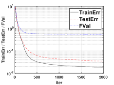
(a)

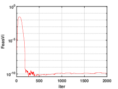
(b)

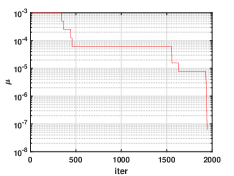
(c)

Figure 2: Algorithm performance of SPG

s

Secondly, we compare SPG with different choices of $L^{(0)}$ on a group of randomly generated data sets with data type 1, $N_{\mathrm{test}}=0$ and $\epsilon_{0}=0.05$. We select three different $\beta$ and four parameter combinations. The numerical results are shown in Figure 3. We can learn from Figure 3 that SPG may diverge if $L^{(0)}$ is not sufficiently large, particularly if $\beta$ is large. When $\beta$ is small, the performance of SPG is not very sensitive to the choice of $L^{(0)}$. We also find that bigger $L^{(0)}$ usually leads to slow convergence. Hence, we can conclude that a suitably selected $L^{(0)}$, such as our default setting, is important to SPG.

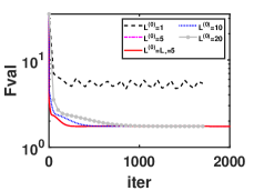
(a) $\beta=1/N$, E.g. 1

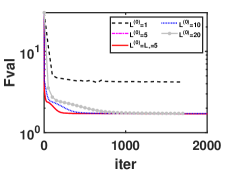
(b) $\beta=1$, E.g. 1

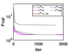
(c) $\beta=10$, E.g. 1

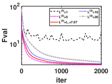
(d) $\beta=1/N$, E.g. 2

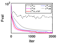
(e) $\beta=1$, E.g. 2

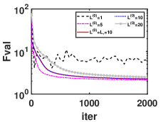
(f) $\beta=10$, E.g. 2

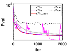
(g) $\beta=1/N$, E.g. 3

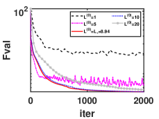
(h) $\beta=1$, E.g. 3

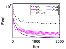
(i) $\beta=10$, E.g. 3

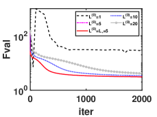
(j) $\beta=1/N$, E.g. 7

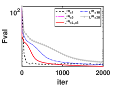
(k) $\beta=1$, E.g. 7

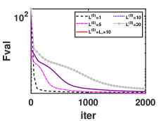
(l) $\beta=10$, E.g. 7

Figure 3: Comparison of SPG with varying $L^{(0)}$.

Finally, we compare SPG with different choices of $\beta$ on a group of randomly generated data sets with $N_{\mathrm{test}}=0$, $\epsilon_{0}=0.05$ and data type 1. We choose $\beta$ from the set $\{\frac{1}{N},\frac{10}{N},\frac{1}{10N},1,10\}$. We record how TrainErr, the FVal and the FeasVi decrease through the iteration. The numerical results with parameter combinations E.g. 4 and E.g. 8 are illustrated in Figures 4 and 5, respectively. We can learn from these two figures that the bigger $\beta$ always leads to slower convergence.

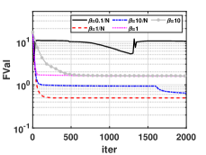
(a)

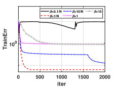
(b)

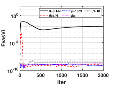
(c)

Figure 4: Comparison of SPG with varying $\beta$, $L^{(0)}=L_{\star}$.

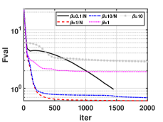
(a)

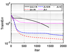
(b)

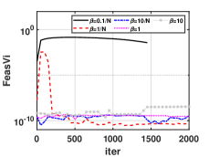
(c)

Figure 5: Comparison of SPG with varying $\beta$, $L^{(0)}=L_{\star}$.

4.3 Comparison with Other Methods

In this subsection, we compare SPG with the existing SGD-based approaches.

We choose two groups of data sets randomly generated by the two data types described in Subsection 4.1, and the numerical results are demonstrated in Figures 6 and 7, respectively. Here, all algorithms start from the same random initial guess. We set $\epsilon_{0}=0.05$ and $N_{\mathrm{test}}=30$. The chosen parameter combinations are given in the subtitles of these two figures.

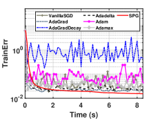
(a) E.g. 5

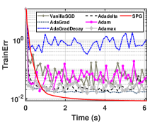
(b) E.g. 6

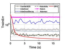
(c) E.g. 9

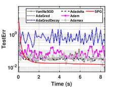
(d) E.g. 5

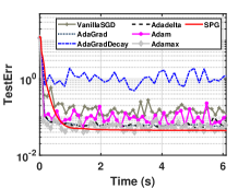
(e) E.g. 6

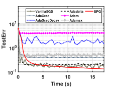
(f) E.g. 9

Figure 6: Comparison among SPG and SGD-based approaches with data type 1.

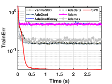
(a) E.g. 5

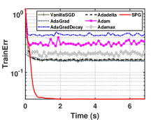
(b) E.g. 6

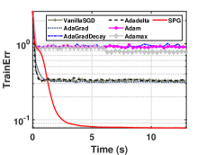
(c) E.g. 9

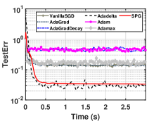
(d) E.g. 5

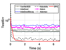
(e) E.g. 6

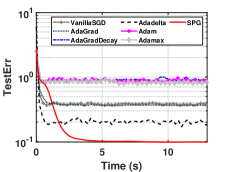
(f) E.g. 9

Figure 7: Comparison among SPG and SGD-based approaches with data type 2.

We can learn from Figures 6 and 7 that SPG reduces the training and test errors slower than some other algorithms at very beginning. It can reach a lower residual than the others finally.

It can also be observed from these two figures that Adadelta outperforms the other SGD-based approaches in the aspects of efficiency and solution quality. Therefore, we consider to use Adadelta as a pre-process to accelerate SPG. More specifically, we first run Adadelta for $1000$ epochs and then switch to SPG. We call the consequent hybrid algorithm SPG-ADA. In the following tests, such pre-processing will be the default setting of SPG.

We select a new group of data sets randomly generated by data type 1 with $N=1000$, $N_{\mathrm{test}}=300$, $\epsilon_{0}=0.05$, and different combinations of $N_{0}$ and $N_{1}$. The iteration number of Adadelta is set as $10000$. We run SPG-ADA and Adadelta $100$ times and record the average output values in Table 1. We can learn from Table 1 that SPG-ADA can obtain better training and test errors than Adadelta in comparable CPU time.

Table 1: Comparison between SPG-ADA and Adadelta with $N=1000$.

		SPG-ADA				Adadelta
$N_{0}$	$N_{1}$	TrainErr	TestErr	FeaErr	Time	TrainErr	TestErr	Time
5	20	3.297e-02	3.636e-02	1.234e-11	8.758	5.518e-02	5.847e-02	3.044
5	30	2.974e-02	3.103e-02	5.599e-12	10.592	5.470e-02	5.566e-02	3.623
5	40	2.960e-02	3.200e-02	7.238e-12	15.206	5.474e-02	5.632e-02	3.786
10	40	6.708e-02	7.727e-02	1.140e-11	19.184	1.257e-01	1.341e-01	5.590
10	60	6.867e-02	7.863e-02	5.138e-11	22.599	1.348e-01	1.436e-01	6.149
10	80	8.105e-02	9.057e-02	8.814e-11	25.701	1.364e-01	1.441e-01	7.169
20	80	1.824e-01	2.200e-01	3.020e-12	33.962	3.766e-01	4.265e-01	8.992
20	120	1.135e-01	2.611e-01	3.634e-12	38.191	4.051e-01	4.566e-01	12.275
20	160	1.946e-01	2.380e-01	2.181e-12	72.942	3.746e-01	4.240e-01	20.268

4.4 Tests on MNIST

In this subsection, we investigate the numerical comparison among SPG-ADA and Adadelta in solving problems arising from the real data set MNIST.

Firstly, we set $N=100$ and $N_{1}=500$. We can find the reconstruction results corresponding to the autoencoder solutions obtained by SPG-ADA and Adadelta in Figure 8 (a)-(b), respectively. We can conclude that SPG-ADA can reach the comparable reconstruction quality as Adadelta. In addition, we also present the reconstruction result derived by Adam, as a failure case. Therefore, we exclude Adam in the last numerical experiment.

(a) SPG-ADA

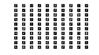
(b) Adadelta

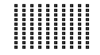
(c) Adam

Figure 8: Reconstruction of MNIST by SPG-ADA, Adadelta and Adam.

Finally, we demonstrate how the training and test errors decrease through the iterations of SPG-ADA and Adadelta. We select different combinations of $N$ and $N_{1}$. The results are illustrated in Figure 9. We can learn that SPG-ADA is much more robust and can always find better solutions.

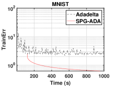
(a) $N=100$, $N_{1}=500$

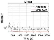
(b) $N=1000$, $N_{1}=1000$

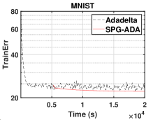
(c) $N=10000$, $N_{1}=2000$

Figure 9: Comparison between SPG-ADA and Adadelta on MNIST.

5 Conclusion

The regularized minimization model (R) using the ReLU activation function has been extensively applied for the autoencoders. However, the set of global minimizers of the model is generally unbounded. Existing algorithms cannot guarantee to generate bounded sequences with decreasing objective function values. In this paper, we propose the regularized minimization model with $l_{1}$-norm penalty (RP) that has same global minimizers, local minimizer and d-stationary points with the regularized minimization model (R). Moreover, we develop the linearly constrained regularized minimization model with $l_{1}$-norm penalty (LRP) which has a bounded solution set contained in the solution sets of (R) and (RP). We develop a smoothing proximal gradient (SPG) algorithm to solve (LRP). We prove the sequence generated by the SPG algorithm is bounded and has a subsequence converging to a generalized d-stationary point of (LRP). We conduct comprehensive numerical experiments to verify the effectiveness, efficiency and robustness of the SPG algorithm.

Finally, we mention that our results on the relationships among (R), (RP), (LRP) can be extended to the following three corresponding problems for training an $L$-layer DNN with ReLU activation functions, given input data $\{x_{n}\}_{n=1}^{N}$ and output data $\{y_{n}\}_{n=1}^{N}$.

(33) $$\min_{z} \,{\cal F}(z)+\mathcal{R}(z)$$

s.t. $$\,u_{n,\ell}=(W_{\ell}u_{n,\ell-1}+b_{\ell})_{+},\quad n=1,\ldots,N,\,\ell=1,\ldots,L,$$

(34) $$\min_{z} \,{\cal F}(z)+\mathcal{R}(z)+\beta\sum_{n=1}^{N}\sum_{\ell=1}^{L}e^{\top}_{N_{\ell}}(u_{n,\ell}-(W_{\ell}u_{n,\ell-1}+b_{\ell})_{+})$$

s.t. $$\,u_{n,\ell}\geq(W_{\ell}u_{n,\ell-1}+b_{\ell})_{+},\quad n=1,\ldots,N,\,\ell=1,\ldots,L,$$

and

(35) $$\min_{z} \,{\cal F}(z)+\mathcal{R}(z)+\beta\sum_{n=1}^{N}\sum_{\ell=1}^{L}e^{\top}_{N_{\ell}}(u_{n,\ell}-(W_{\ell}u_{n,\ell-1}+b_{\ell})_{+})$$

s.t. $$\,u_{n,\ell}\geq(W_{\ell}u_{n,\ell-1}+b_{\ell})_{+},\,\,\|b_{\ell}\|_{\infty}\leq\alpha_{\ell},\quad n=1,\ldots,N,\,\ell=1,\ldots,L,$$

respectively, where $\alpha_{\ell}$ is a given constant, $u_{n,0}=x_{n}$, ${\cal F}(z)=\frac{1}{N}\sum^{N}_{n=1}\|(W_{L}u_{n,L}+b_{L})_{+}-y_{n}\|^{2}_{2}$, ${\cal R}(z)=\lambda_{1}\sum_{n=1}^{N}\sum^{L}_{\ell=1}e^{T}_{N_{\ell}}u_{n,l}+\lambda_{2}\sum^{L}_{\ell=1}||W_{\ell}\|_{F}^{2}$,

$$z=(\mathrm{vec}(W_{1})^{\top},\ldots,\mathrm{vec}(W_{L})^{\top},u_{1,1}^{\top},u_{2,1}^{\top},\ldots,u_{N,1}^{\top},u_{1,2}^{\top},\ldots,u_{N,L}^{\top},b_{1}^{\top},\ldots,b_{L}^{\top})^{\top},$$

for all $\ell=1,2,\ldots,L$ and $n=1,2,\ldots,N$. However, the increasing number of layers results in more rapidly increasing number of variables which requires further development on the algorithm to maintain the numerical comparability to SGD-based approaches.

Acknowledgements. The authors would like to thank the reviewers for their insightful comments and efforts towards improving our manuscript.

Appendix A Proof of Lemma 3.2

Proof A.1.

$($a$)$ It follows from the updating formula (26) of $\mu$ and $L$, the required relations (27) and $\tau_{1}\tau_{3}\geq 1$ that

(36) $$\mu^{(k)}L^{(k)}\geq\mu^{(0)}L^{(0)}\geq\max\left\{6\lambda_{2}N_{1}N_{0}+\frac{2}{\eta}(N_{2}L_{\widetilde{\mathcal{H}}}+\lambda_{1}N_{1}N),8\lambda_{2}+L_{\nabla\widetilde{\mathcal{H}}}\right\}$$

holds for all $k=0,1,\ldots$.

Next, we use the mathematical induction to prove the facts that $\{z^{(k)}\}\subset\Omega_{\theta}\cap{\cal Z}$ and $\{\widetilde{\mathcal{O}}(z^{(k)},\mu^{(k)})\}$ is non-increasing. Naturally, we have $z^{(0)}\in\Omega_{\theta}\cap{\cal Z}$. Then we suppose that $z^{(k)}\in\Omega_{\theta}\cap{\cal Z}$ and $\widetilde{\mathcal{O}}(z^{(l)},\mu^{(l)})\leq\widetilde{\mathcal{O}}(z^{(l-1)},\mu^{(l-1)})$ hold for all $l=1,2,\ldots,k$.

We deduce from $z^{(k)}\in\Omega_{\theta}\cap{\cal Z}$ and the proof of Lemma 2.2 that $\|b^{(k)}\|_{\infty}\leq\alpha$ and $\|z^{(k)}-[0,0,(b^{(k)})^{\top}]^{\top}\|_{\infty}\leq\eta$. If $\|z^{(k+1)}-[0,0,(b^{(k)})^{\top}]^{\top}\|_{\infty}>2\eta$, we immediately have $\bar{\eta}:=\|z^{(k+1)}-z^{(k)}\|_{\infty}>\eta$. Then, it holds that

$$\left\langle\nabla_{z}\widetilde{\mathcal{H}}(z^{(k)},\mu^{(k)}),z^{(k+1)}-z^{(k)}\right\rangle+\mathcal{R}(z^{(k+1)})-\mathcal{R}(z^{(k)})+\frac{L^{(k)}}{2}\|z^{(k+1)}-z^{(k)}\|_{2}^{2}$$

$$\geq -N_{2}\frac{L_{\widetilde{\mathcal{H}}}}{\mu^{(k)}}\bar{\eta}+\frac{L^{(k)}}{2}\bar{\eta}^{2}+\mathcal{R}(z^{(k+1)})-\mathcal{R}(z^{(k)})$$

$$\geq -N_{2}\frac{L_{\widetilde{\mathcal{H}}}}{\mu^{(k)}}\bar{\eta}+\frac{L^{(k)}}{2}\bar{\eta}^{2}-\lambda_{1}N_{1}N\bar{\eta}-\lambda_{2}N_{0}N_{1}\bar{\eta}\max_{j\in\{1,2,\ldots,N_{1}\}}\|W_{\cdot,j}^{(k+1)}+W_{\cdot,j}^{(k)}\|_{\infty}$$

$$\geq -N_{2}\frac{L_{\widetilde{\mathcal{H}}}}{\mu^{(k)}}\bar{\eta}+\frac{L^{(k)}}{2}\bar{\eta}^{2}-\lambda_{1}N_{1}N\bar{\eta}-\lambda_{2}N_{0}N_{1}\bar{\eta}\left(\bar{\eta}+2\eta\right)>0,$$

where the second inequality comes from the definition of $\mathcal{R}$, the third inequality results from the relations $\|W_{\cdot,j}^{(k+1)}+W_{\cdot,j}^{(k)}\|_{\infty}\leq\|W_{\cdot,j}^{(k+1)}-W_{\cdot,j}^{(k)}\|_{\infty}+2\|W_{\cdot,j}^{(k)}\|_{\infty}\leq\bar{\eta}+2\eta$ for all $j=1,2,\ldots,N_{1}$, and the last inequality comes from $0<\mu^{(k)}<1$ and (36). This leads to a contradiction, since $z^{(k+1)}$ is a solution of subproblem (25). Hence, we have $\|z^{(k+1)}\|_{\infty}\leq\max\{\alpha,2\eta\}$.

By the KKT condition of (25), there exists a nonnegative vector $\gamma^{{(k+1)}}\in\mathbb{R}^{\nu}$ such that

(37) $$\left\{\begin{aligned} &\nabla_{z}\widetilde{\mathcal{H}}(z^{(k)},\mu)+\nabla\mathcal{R}(z^{(k+1)})+A^{\top}\gamma^{{(k+1)}}+L^{(k)}(z^{(k+1)}-z^{(k)})=0,\\ &Az^{(k+1)}\leq c,(\gamma^{{(k+1)}})^{\top}(Az^{(k+1)}-c)=0.\end{aligned}\right.$$

It follows from the inequality (36), the relations (37), $(\gamma^{{(k+1)}})^{\top}(Az^{(k)}-c)\leq 0$, $0<\mu^{(k)}\leq 1$ and the definition of $L_{\nabla\widetilde{\mathcal{H}}}$ that

(38) $$\widetilde{\mathcal{O}}(z^{(k+1)},\mu^{(k)})-\widetilde{\mathcal{O}}(z^{(k)},\mu^{(k)})$$

$$\leq \left\langle\nabla_{z}\widetilde{\mathcal{O}}(z^{(k)},\mu^{(k)}),z^{(k+1)}-z^{(k)}\right\rangle+\frac{2\lambda_{2}+L_{\nabla\widetilde{\mathcal{H}}}}{2\mu^{(k)}}\|z^{(k+1)}-z^{(k)}\|_{2}^{2}$$

$$= \left\langle\nabla\mathcal{R}(z^{(k)})-\nabla\mathcal{R}(z^{(k+1)})-A^{\top}\gamma^{{(k+1)}}-L^{(k)}(z^{(k+1)}-z^{(k)}),z^{(k+1)}-z^{(k)}\right\rangle$$

$$+\frac{2\lambda_{2}+L_{\nabla\widetilde{\mathcal{H}}}}{2\mu^{(k)}}\|z^{(k+1)}-z^{(k)}\|_{2}^{2}$$

$$\leq \frac{2\lambda_{2}+L_{\nabla\widetilde{\mathcal{H}}}-2\mu^{(k)}L^{(k)}}{2\mu^{(k)}}\|z^{(k+1)}-z^{(k)}\|_{2}^{2}-\left\langle A^{\top}\gamma^{{(k+1)}},z^{(k+1)}-z^{(k)}\right\rangle+2\lambda_{2}\|z^{(k+1)}-z^{(k)}\|^{2}_{2}$$

$$\leq \frac{6\lambda_{2}+L_{\nabla\widetilde{\mathcal{H}}}-2\mu^{(k)}L^{(k)}}{2\mu^{(k)}}\|z^{(k+1)}-z^{(k)}\|_{2}^{2}+(\gamma^{{(k+1)}})^{\top}(Az^{(k)}-c)\leq 0.$$

Due to the nondecreasing property of $\{\widetilde{\mathcal{O}}(z^{(k+1)},\mu)\}$ with respect to smoothing parameter $\mu$, we have $\widetilde{\mathcal{O}}(z^{(k+1)},\mu^{(k+1)})\leq\widetilde{\mathcal{O}}(z^{(k+1)},\mu^{(k)})$ with $\mu^{(k+1)}\leq\mu^{(k)}$. Together with the relations (24) and (38), we arrive at $\widetilde{\mathcal{O}}(z^{(k+1)},\mu^{(k+1)})\leq\widetilde{\mathcal{O}}(z^{(k)},\mu^{(k)})$ and $\mathcal{O}(z^{(k+1)})<\theta$. Besides, it follows from the definition of $z^{(k+1)}$ that $z^{(k+1)}\in\mathcal{Z}$. Hence, we have $z^{(k+1)}\in\Omega_{\theta}\cap{\cal Z}$ and $\widetilde{\mathcal{O}}(z^{(l)},\mu^{(l)})\leq\widetilde{\mathcal{O}}(z^{(l-1)},\mu^{(l-1)})$ hold for all $l=1,2,\ldots,k+1$. This completes the part (a) by mathematical induction.

$($b$)$ By what we have proved in $($a$)$ and the inequality $\widetilde{\mathcal{O}}(z^{(k+1)},\mu^{(k)})-\widetilde{\mathcal{O}}(z^{(k)},\mu^{(k)})\geq-\tau_{2}\frac{\mu^{(k)}}{L^{(k)}}$, we can obtain that

$$-\tau_{2}\frac{\mu^{(k)}}{L^{(k)}}\leq\frac{6\lambda_{2}+L_{\nabla\widetilde{\mathcal{H}}}-2\mu^{(k)}L^{(k)}}{2\mu^{(k)}}\|z^{(k+1)}-z^{(k)}\|_{2}^{2}+(\gamma^{{(k+1)}})^{\top}(Az^{(k)}-c).$$

which together with the relations $(\gamma^{{(k+1)}})^{\top}(Az^{(k)}-c)\leq 0$ and $\mu^{(k)}L^{(k)}>8\lambda_{2}+L_{\nabla\widetilde{\mathcal{H}}}$ further implies that

(39) $$\|z^{(k+1)}-z^{(k)}\|_{2}^{2}\leq\frac{2\tau_{2}(\mu^{(k)})^{2}}{L^{(k)}(2\mu^{(k)}L^{(k)}-6\lambda_{2}-L_{\nabla\widetilde{\mathcal{H}}})},$$

(40) $$-\tau_{2}\frac{(\mu^{(k)})^{2}}{8\lambda_{2}+L_{\nabla\widetilde{\mathcal{H}}}}\leq(\gamma^{{(k+1)}})^{\top}(Az^{(k)}-c)\leq 0.$$

It follows from the inequality (39) and the KKT condition (37) that

$$\left\|\nabla\widetilde{\mathcal{O}}(z^{(k)},\mu^{(k)})+A^{\top}\gamma^{{(k+1)}}\right\|_{2}=\left\|\nabla\mathcal{R}(z^{(k)})-\nabla\mathcal{R}(z^{(k+1)})-L^{(k)}(z^{(k+1)}-z^{(k)})\right\|_{2}$$

$$\leq \left\|\nabla\mathcal{R}(z^{(k)})-\nabla\mathcal{R}(z^{(k+1)})\right\|_{2}+L^{(k)}\left\|z^{(k+1)}-z^{(k)}\right\|_{2}\leq(2\lambda_{2}+L^{(k)})\left\|z^{(k+1)}-z^{(k)}\right\|_{2}$$

$$\leq \sqrt{\frac{2\tau_{2}}{L^{(k)}(2\mu^{(k)}L^{(k)}-6\lambda_{2}-L_{\nabla\widetilde{\mathcal{H}}})}}\mu^{(k)}(2\lambda_{2}+L^{(k)})\,\leq\,2\sqrt{\tau_{2}}(\mu^{(k)})^{1/2},$$

where the last inequality results from the inequalities $0<\mu^{(k)}<1$, $\mu^{(k)}L^{(k)}>8\lambda_{2}+L_{\nabla\widetilde{\mathcal{H}}}$ and $L^{(k)}>2\lambda_{2}$. Together with (40), we can conclude the proof.

Appendix B A Structured Algorithm for Solving (25)

We notice that the subproblem (25) is a convex quadratic programming (QP), which can be solved by any QP solvers such as ‘quadprog’ [35], the default QP solver in MATLAB, and ‘CVX’ [15]. Since the subproblem of our SPG to be solved in autoencoder scenario is usually large-scale but structured, the existing solvers are not efficient enough. Therefore, in this subsection we propose a special algorithm for subproblem  (25) to take the structure into account. We focus on this subproblem at the $k$-th iteration of SPG for any $k=0,1,...$. For brevity, we will drop the superscript $(k)$ and let $(\bar{W},\bar{b},\bar{V})$ to denote the current iterate $(W^{(k)},b^{(k)},V^{(k)})$ (and similarly for $\mu^{(k)}$ and $L^{(k)}$) in this section. In addition, we introduce a new group of variables $U=(u_{1},u_{2},\ldots,u_{N})$ subject to $u_{n}=Wx+b_{1}$ for all $n=1,...,N$. Hence the quadratic programming (25) can be reformulated as

(41) $$\min_{W,b,V,U,\rho} \,\,\left\langle g_{W},W-\bar{W}\right\rangle+\left\langle g_{b},b-\bar{b}\right\rangle+\left\langle g_{V},V-\bar{V}\right\rangle+\lambda_{1}\|W\|_{F}^{2}+\lambda_{2}\sum_{n=1}^{N}e^{\top}v_{n}+\frac{L}{2}\|z-\bar{z}\|_{2}^{2}$$

s.t. $$\,\,\,\,\,b\in\Omega_{3},v_{n}\geq u_{n},\,\,v_{n}\geq 0,\,\,u_{n}=Wx+b_{1},\,\,\mbox{ for\, all\, }n=1,2,\ldots,N,$$

where $g_{W}=\nabla_{W}\widetilde{\mathcal{H}}(\bar{W},\bar{b},\bar{V},\mu),$ $g_{V}=\nabla_{V}\widetilde{\mathcal{H}}(\bar{W},\bar{b},\bar{V},\mu),$ and $g_{b}=\nabla_{b}\widetilde{\mathcal{H}}(\bar{W},\bar{b},\bar{V},\mu)$ are preset constants in this subproblem.

The variables of problem (41) can be divided into two parts $(W,b)$ and $(V,U)$. We then apply the alternating direction method of multipliers (ADMM) to solve (41). By penalizing the equality constraints, we obtain the augmented Lagrange penalty function

$$\mathcal{G}(W,b,V,U,\rho):= \lambda_{1}\|W\|_{F}^{2}+\lambda_{2}\sum_{n=1}^{N}e^{\top}v_{n}+\left\langle g_{W},W-\bar{W}\right\rangle+\left\langle g_{b},b-\bar{b}\right\rangle+\left\langle g_{V},V-\bar{V}\right\rangle$$

$$+\sum_{n=1}^{N}\left\langle\rho_{n},u_{n}-(Wx_{n}+b_{1})\right\rangle+\frac{1}{2}\sum_{n=1}^{N}\|u_{n}-(Wx_{n}+b_{1})\|_{2}^{2}+\frac{L}{2}\|z-\bar{z}\|_{2}^{2},$$

where $\rho=(\rho_{1},\rho_{2},\ldots,\rho_{N})$ with $\rho_{n}\in\mathbb{R}^{N_{1}}$, for all $n=1,...,N$, are the Lagrangian multipliers associated with the equality constraints.

At the $l$-th iteration, we first fix $W=W^{(l)}$, $b=b^{(l)},\rho=\rho^{(l)}$, and the $(V,U)$ subproblem can be formulated as

$$\min_{U,V} \mathcal{G}(W^{(l)},b^{(l)},V,U,\rho^{(l)})$$

s.t. $$v_{n}\geq u_{n},\,\,v_{n}\geq 0,\text{ for all }n=1,2,\ldots,N.$$

Due to the separability of $v_{n}$ and $u_{n}$ for all $n=1,...,N$, the $(V,U)$ subproblem has also a closed-form solution, which is illustrated as follows,

(42) $$\left\{\begin{aligned} &V^{(l+1)}_{j,n}=-\xi_{j,n}^{1;l},U^{(l+1)}_{j,n}=-\xi_{j,n}^{2;l},\quad\text{ if }\xi_{j,n}^{2;l}\geq\xi_{j,n}^{1;l}\text{ and }\xi_{j,n}^{1;l}\leq 0,\\ &V^{(l+1)}_{j,n}=0,U^{(l+1)}_{j,n}=-\xi_{j,n}^{2;l},\hskip 26.01724pt\text{ if }\xi_{j,n}^{2;l}\geq 0,\xi_{j,n}^{1;l}>0,\\ &V^{(l+1)}_{j,n}=U^{(l+1)}_{j,n}=0,\hskip 52.03448pt\text{ if }\xi_{j,n}^{2;l}<0,\text{ and }L\xi_{j,n}^{1;l}+\xi_{j,n}^{2;l}>0,\\ &V^{(l+1)}_{j,n}=U^{(l+1)}_{j,n}=-\frac{L\xi_{j,n}^{1;l}+\xi_{j,n}^{2;l}}{L+1},\hskip 0.72229pt\text{ otherwise}\end{aligned}\right.$$

for all $j=1,2,\ldots,N_{1}$ and $n=1,2,\ldots,N$. Here, $\xi_{n}^{1;l}=g_{v_{n}}/L-\bar{v}_{n}+\lambda_{2}e/L$, $\xi_{n}^{2;l}=\rho^{(l)}_{n}-(W^{(l)}x_{n}+b^{(l)}_{1})$, $g_{v_{n}}$ is the $n$-th column of $g_{V}$, and $\xi_{j,n}^{1;l}$ and $\xi_{j,n}^{2;l}$ are the $j$-th elements of $\xi_{n}^{1;l}$ and $\xi_{n}^{2;l}$, respectively, for all $j=1,2,\ldots,N_{1}$ and $n=1,2,\ldots,N$.

Secondly, we fix $V=V^{(l+1)}$, $U=U^{(l+1)},\rho=\rho^{(l)}$, and then the $(W,b)$ subproblem can be written as

$$\min_{W,b\in\Omega_{3}} \mathcal{G}(W,b,V^{(l+1)},U^{(l+1)},\rho^{(l)}).$$

By simply calculation, we can obtain its closed-form solution as follows.

(43) $$W^{(l+1)}=\widehat{W}^{(l+1)}\widetilde{I}^{\top},\,\mbox{and}\quad b^{(l+1)}=\mathrm{Proj}_{\Omega_{3}}(\widehat{W}^{(l+1)}s_{N_{0}+1},\bar{b}_{2}-g_{b_{2}}/L),$$

where

$$\widehat{W}^{(l+1)}=\left(-[g_{W},g_{b_{1}}]+L[\bar{W},\bar{b}_{1}]+\rho^{(l)}\widehat{X}^{\top}+U^{(l+1)}\widehat{X}^{\top}\right)\left(LI_{N_{0}+1}+2\lambda_{1}\widetilde{I}^{\top}\widetilde{I}+\widehat{X}\widehat{X}^{\top}\right)^{-1},$$

$s_{N_{0}+1}=(0,0,\ldots,0,1)\in\mathbb{R}^{N_{0}+1}$, $[g_{b_{1}}^{\top},g_{b_{2}}^{\top}]=g_{b}^{\top}$, $\widehat{X}:=(X^{\top},1_{N})^{\top}$ and $\widetilde{I}=[I_{N_{0}},0]$.

Finally, we present the framework of ADMM for solving the subproblem (25).

Algorithm 2 A Splitting and Alternating Method for the Quadratic Programming (25) (SAMQP)

1:   Initialization: set $(W^{(l)},b^{(l)},V^{(l)})=(\bar{W},\bar{b},\bar{V})$, $\rho^{(l)}=0$, $u^{(l)}_{n}=W^{(l)}x_{n}+b^{(l)}_{1}$ for all $n=1,...,N$, and $l:=0$.

2:  while the stop criterion is not met do

3:     Calculate $V^{(l+1)},U^{(l+1)}$ by (42);

4:     Calculate $W^{(l+1)},b^{(l+1)}$ by (43);

5:     Calculate $\rho_{n}^{(l+1)}=\rho_{n}^{(l)}+(u^{(l+1)}_{n}-(W^{(l+1)}x_{n}+b^{(l+1)}_{1}))$, for all $n=1,2,\ldots,N$;

6:     Set $l:=l+1$.

7:  end while

Since the subproblem (25) is strongly convex, any sequence generated by SAMQP, a two block ADMM, converges to a global solution of (25). Furthermore, the local R-linear rate convergence of SAMQP can be guaranteed by Boley [2].

To test the efficiency of SAMQP, we construct the following randomly generated test problems. We set $X=\mathrm{rand}(N_{0},N)$, $g_{W}=\mathrm{rand}(N_{1},N_{0})$, $g_{b}=\mathrm{rand}(N_{1}+N_{0},1)$, $g_{V}=\mathrm{rand}(N_{1},N)$, $\bar{W}=\mathrm{randn}(N_{1},N_{0})/N$, $\bar{V}_{n}=(\bar{W}x_{n})_{+}$ for all $n=1,2,\ldots,N$ and $\bar{b}=0$. The problem parameters $\mu$ and $L$ are set as $0.001$ and $1$, respectively. In addition, the stopping criterion is set as

$$\max\left\{\|\rho^{(l+1)}-\rho^{(l)}\|_{F}^{2},\|U^{(l+1)}-U^{(l)}\|_{F}^{2}\right\}\leq 10^{-6}.$$

We compare SAMQP with some existing QP solvers including the ‘quadprog’ solver from MATLAB, the ‘fmincon’ solver from MATLAB and the ‘CVX’ solver [15] for solving (25). We choose seven test problems with different sizes. We record the CPU time in seconds required by these solvers. The results are displayed in Table 2, in which “–” stands for the cases that the solver runs out of memory during the iteration or terminates abnormally. It can be easily observed that SAMQP is the most efficient and robust one among these four solvers.

Table 2: A comparison of CPU time for several solvers and SAMQP.

				CPU time (s)
$N$	$N_{1}$	$N_{0}$	$N_{2}$	‘fmincon’	‘quadprog’	‘CVX’	SAMQP
100	5	5	535	3.502	0.707	2.031	0.099
100	10	10	1120	33.990	4.546	1.172	0.105
100	20	20	2440	674.163	39.303	1.781	0.189
100	40	40	5680	–	359.555	6.672	0.419
100	100	10	11110	–	–	7.453	0.838
1000	100	10	101110	–	–	50.781	6.056
10000	784	1000	8625784	–	–	–	189.868

References

- [1] A. F. Agarap, Deep learning using rectified linear units (ReLU), preprint, arxiv:1803.08375, (2018).
- [2] D. Boley, Local linear convergence of the alternating direction method of multipliers on quadratic or linear programs, SIAM J. Optim., 23 (2013), pp. 2183–2207.
- [3] H. Bourlard and Y. Kamp, Auto-association by multilayer perceptrons and singular value decomposition, Biol. Cybern., 59 (1988), pp. 291–294.
- [4] J. Burke, X. Chen, and H. Sun, The subdifferential of measurable composite max integrands and smoothing approximation, Math. Program., 181 (2020), pp. 229–264.
- [5] M. Carreira-Perpinan and W. Wang, Distributed optimization of deeply nested systems, in Proceedings of the 17th International Conference on Artificial Intelligence and Statistics, 2014, pp. 10–19.
- [6] X. Chen, Smoothing methods for nonsmooth, nonconvex minimization, Math. Program., 134 (2012), pp. 71–99.
- [7] X. Chen, Z. Lu, and T. K. Pong, Penalty methods for a class of non-Lipschitz optimization problems, SIAM J. Optim., 26 (2016), pp. 1465–1492.
- [8] F. H. Clarke, Optimization and Nonsmooth Analysis, vol. 5, SIAM, Philadelphia, 1990.
- [9] H. Cramir, Mathematical methods of statistics, Princeton U. Press, Princeton, (1946), p. 500.
- [10] Y. Cui, Z. He, and J.-S. Pang, Multicomposite nonconvex optimization for training deep neural networks, SIAM J. Optim., 30 (2020), pp. 1693–1723.
- [11] G. E. Dahl, T. N. Sainath, and G. E. Hinton, Improving deep neural networks for LVCSR using rectified linear units and dropout, in 2013 IEEE International Conference on Acoustics, Speech and Signal Processing, pp. 8609–8613.
- [12] J. Duchi, E. Hazan, and Y. Singer, Adaptive subgradient methods for online learning and stochastic optimization, J. Mach. Learn. Res., 12 (2011), pp. 2121–2159.
- [13] X. Glorot, A. Bordes, and Y. Bengio, Deep sparse rectifier neural networks, in Proceedings of the 14th International Conference on Artificial Intelligence and Statistics, 2011, pp. 315–323.
- [14] I. Goodfellow, Y. Bengio, A. Courville, and Y. Bengio, Deep Learning, vol. 1, MIT press Cambridge, 2016.
- [15] M. Grant and S. Boyd, CVX: Matlab software for disciplined convex programming, version 2.1, 2014.
- [16] G. E. Hinton and R. R. Salakhutdinov, Reducing the dimensionality of data with neural networks, Science, 313 (2006), pp. 504–507.
- [17] A. J. Hoffman, On approximate solutions of systems of linear inequalities, in Selected Papers of Alan J Hoffman: With Commentary, World Scientific, 2003, pp. 174–176.
- [18] K. Jarrett, K. Kavukcuoglu, M. Ranzato, and Y. LeCun, What is the best multi-stage architecture for object recognition?, in 2009 IEEE 12th international conference on computer vision, 2009, pp. 2146–2153.
- [19] H. Kasai, SGDLibrary: A MATLAB library for stochastic optimization algorithms, J. Mach. Learn. Res., 18 (2018), pp. 1–5.
- [20] D. P. Kingma and J. Ba, Adam: A method for stochastic optimization, preprint, arxiv:1412.6980, (2014).
- [21] A. Krogh and J. A. Hertz, A simple weight decay can improve generalization, in Advances in Neural Information Processing Systems, 1992, pp. 950–957.
- [22] T. T.-K. Lau, J. Zeng, B. Wu, and Y. Yao, A proximal block coordinate descent algorithm for deep neural network training, preprint, arXiv:1803.09082, (2018).
- [23] Y. Le Cun and F. Fogelman-Soulié, Modèles connexionnistes de l’apprentissage, Intellectica, 2 (1987), pp. 114–143.
- [24] Y. LeCun, The MNIST database of handwritten digits, (1998).
- [25] Y. LeCun, L. Bottou, Y. Bengio, and P. Haffner, Gradient-based learning applied to document recognition, Proceedings of the IEEE, 86, pp. 2278–2324.
- [26] P. Li and P.-M. Nguyen, On random deep weight-tied autoencoders: Exact asymptotic analysis, phase transitions, and implications to training, in Proceedings of the International Conference on Learning Representations, 2019.
- [27] A. L. Maas, A. Y. Hannun, and A. Y. Ng, Rectifier nonlinearities improve neural network acoustic models, in Proceedings of the 30-th International Conference on Machine Learning, vol. 30, 2013, p. 3.
- [28] W. S. McCulloch and W. Pitts, A logical calculus of the ideas immanent in nervous activity, The Bulletin of Mathematical Biophysics, 5 (1943), pp. 115–133.
- [29] R. Mifflin, Semismooth and semiconvex functions in constrained optimization, SIAM J. Control Optim., 15 (1977), pp. 959–972.
- [30] V. Nair and G. E. Hinton, Rectified linear units improve restricted boltzmann machines, in Proceedings of the 27-th International Conference on Machine Learning, 2010.
- [31] A. Ng, Sparse autoencoder, CS294A Lecture Notes, 72 (2011), pp. 1–19.
- [32] L. Pasa and A. Sperduti, Pre-training of recurrent neural networks via linear autoencoders, in Advances in Neural Information Processing Systems, 2014, pp. 3572–3580.
- [33] R. Sun, Optimization for deep learning: theory and algorithms, preprint, arxiv:1912.08957, (2019).
- [34] G. Taylor, R. Burmeister, Z. Xu, B. Singh, A. Patel, and T. Goldstein, Training neural networks without gradients: A scalable admm approach, in Proceedings of the 33rd International Conference on Machine Learning, 2016, pp. 2722–2731.
- [35] M. A. Weingessel, The quadprog package, (2007).
- [36] L. Wen, L. Gao, and X. Li, A new deep transfer learning based on sparse auto-encoder for fault diagnosis, IEEE Transactions on systems, man, and cybernetics: systems, 49 (2017), pp. 136–144.
- [37] Y. Xu, X. Liu, X. Cao, C. Huang, E. Liu, S. Qian, X. Liu, Y. Wu, F. Dong, C.-W. Qiu, et al., Artificial intelligence: A powerful paradigm for scientific research, The Innovation, 2 (2021), p. 100179.
- [38] M. D. Zeiler, Adadelta: an adaptive learning rate method, preprint, arXiv:1212.5701, (2012).
- [39] J. Zeng, T. T.-K. Lau, S. Lin, and Y. Yao, Global convergence of block coordinate descent in deep learning, in Proceedings of the 36th International Conference on Machine Learning, 2019, pp. 7313–7323.