Nikhef-2021-006, LTH-1254
Five loop renormalization of theory with applications to the Lee–Yang edge singularity and percolation theory
bTheoretical Physics Division, Department of Mathematical Sciences,
University of Liverpool, P.O. Box 147, Liverpool, L69 3BX, United Kingdom
cSt. Petersburg State University, 7/9 Universitetskaya nab.,
St. Petersburg 199034, Russia
dDepartment Mathematik, Friedrich Alexander Universität Erlangen-Nürnberg,
Cauerstraße 11, 91058 Erlangen, Germany)
Abstract
We apply the method of graphical functions that was recently extended to six dimensions for scalar theories, to theory and compute the function, the wave function anomalous dimension as well as the mass anomalous dimension in the scheme to five loops. From the results we derive the corresponding renormalization group functions for the Lee–Yang edge singularity problem and percolation theory. After determining the expansions of the respective critical exponents to we apply recent resummation technology to obtain improved exponent estimates in , and dimensions. These compare favourably with estimates from fixed dimension numerical techniques and refine the four loop results. To assist with this comparison we collated a substantial amount of data from numerical techniques which are included in tables for each exponent.
1 Introduction
One of the core quantum field theories with applications to various areas of physics is that of a scalar field with a cubic self-interaction. It has many interesting properties. For instance, it is known to be asymptotically free in six dimensions [1, 2] which is also its critical dimension. As such it offered a much simpler forum to study this property rather than in the more complicated non-abelian gauge field theory underlying the strong interactions which also has this property. Another major area where scalar theory has important consequences is that of condensed matter physics. For example, the non-unitary version of the model, [3], describes the phase transitions of the Lee–Yang edge singularity problem. In particular the critical exponents computed in the cubic theory produce estimates which are not out of line with those of other methods, [4, 5]. Having an accurate estimate for the exponent for the Lee–Yang edge singularity is important in lattice gauge theory studies of Quantum Chromodynamics (QCD), [6, 7]. Specifically it governs the analytic behaviour of the partition function in the smooth chiral symmetry crossover when there is a non-zero chemical potential. The latter is included in QCD as an purely imaginary parameter that leads to loss of unitarity. Though for the region of application in [6, 7] physical meaningful results can still be extracted. In addition endowing the cubic model with specific symmetries means it can also describe phase transitions in percolation problems. This follows from taking the replica limit of the -state Potts model [8]. The critical dynamics of the phase transition in percolation has been widely studied using Monte Carlo or series methods, on discrete or spin systems. References for this comprehensive body of work will be provided in later sections. Indeed such analyses proceed over a range of integer dimensions from to inclusive where the latter would correspond to the mean field approximation given its relation to the critical dimension. The relation of the discrete percolation theory models to that of a continuum field theory resides in the fact that at the phase transition both scalar theory and the spin models lie in the same universality class. What differs of course in both approaches are the techniques used to estimate the physically measurable critical exponents. On the continuum quantum field theory side these are renormalization group invariants that are determined from high perturbative loop order renormalization group functions. While these functions are scheme dependent, the critical exponents at the dimensional Wilson–Fisher fixed point, [9], are scheme independent. In more recent years other continuum field theory techniques have been developed. Two of the main ones are the functional renormalization group and the modern manifestation of the conformal bootstrap and applied to the Lee–Yang and percolation problem for example in [10, 11, 12] and [13, 14, 15] respectively.
In terms of basic scalar theory the multiloop renormalization of the model has proceeded in stages over the last half century or so. The one and two loop renormalization group functions were determined in [1]. This was extended to the group in [2] where the leading order value of for the existence of the conformal window was determined. The extension to three loops for both the Lee–Yang edge singularity and percolation problems was carried out in [4, 5]. From the point of view of hindsight that computation was well ahead of its time given the difficulty of several of the three loop vertex graphs that needed to be evaluated. Moreover, estimates for the exponents in the percolation and Lee–Yang problems were extracted in dimensions in the range that were competitive with other results available then. To achieve a high degree of accuracy the analysis benefited from improved resummation techniques such as Padé approximants and Borel transformations, where in the latter conformal mappings were applied and the behaviour of the expansion was incorporated. Thereafter progress in systematically renormalizing theories to higher loop order was hindered in general by a lack of technology to push to four loops. Indeed three loop calculations were only viable due to the integration by parts (IBP) method introduced in [16]. However, with the development of Laporta’s integration by parts algorithm, [17], and its implementation within a variety of publicly available packages, the four loop renormalization of was carried out in [18]. That article covered a range of applications to various problems that had emerged in the interim. For instance, in recent years it has been shown that there is a connection of theory with dualities in higher spin AdS/CFTs, [19, 20]. This generated an interest in understanding the conformal window of theories for various symmetry groups such as and , [21, 22, 23]. One highlight of the four loop result of [18] was the improvement in estimates for the Lee–Yang and percolation theory exponents. What this analysis benefited immensely from was the progress in classifying two dimensional conformal field theories in the years after [4, 5]. Specifically the values of the exponents of each problem in two dimensions were found exactly. For instance, the exponent in one and two dimensions was determined exactly in [24]. For percolation theory the two dimensional values can be derived from the unitary minimal conformal field theories of [25] when and the central charge is . Therefore it was possible to use that data, together with hyperscaling relations, to construct constrained Padé approximants motivated by the application of this idea given in [26]. The upshot was that exponent estimates based on four loop results for three dimensions were within one standard deviation of Monte Carlo and series results. This is all the more remarkable when one recalls this is the resummation of a series that is more reliable near six dimensions down to three dimensions. We note that for brevity we will refer to results from non-continuum field theories as Monte Carlo but this will cover those from series methods too. We note that in this respect we have compiled exponent estimates from as many sources as we could. These will also include strong coupling methods, functional renormalization group techniques and several specialized approaches. An excellent live source for percolation exponents is [27].
While the Laporta approach has revolutionized our ability to extend results for many theories to loop orders that what would have been impossible to conceive of a decade ago, one is always interested in going beyond even those orders. In the short term any such developments have to proceed in simpler theories. Indeed this has been the case for scalar theory which was renormalized at five loops in the ’s in [28, 29] but not extended to six loops until around a quarter of a century later, [30, 31]. Moreover the latter article [31] contained a most comprehensive analysis of the resummation of exponents using the asymptotic properties of the series. Such an analysis was much-needed after the huge jump in precision. Indeed it revisited the assumptions made in earlier approaches in the literature. Subsequent to [30, 31] a novel method was applied to scalar theory in [32] which is termed graphical functions. This extended the renormalization group functions to the staggeringly high seven loop order111 The eight loop evaluation of the field anomalous dimension has now been determined [33]. . One highlight was the appearance of a new period in the function which is conjectured to not be expressible in terms of a multiple zeta value (MZV), [34, 32]. En route expectations concerning the non-MZV content predicted in [35] at high loop order were confirmed.
One lesson from [32] was the potential usefulness of the graphical function technique to extend the renormalization group functions. An obstruction that limited the technique to four dimensional problems was overcome by the first and fourth author, who extended the method to arbitrary even dimensions. The details of this extension will be given elsewhere [36]. This availability of graphical functions in arbitrary even dimensions immediately opened up new possibilities for the computation of the renormalization group functions in theory in six dimensions. In this article we make use of this new tool and provide the renormalization group functions of theory up to five loops. We emphasise that we will make no use at all of integration by parts in our computation. Consequently we will find the next term in the expansion of the critical exponents for the Lee–Yang singularity and percolation problems. This will form the first part of the article. The second part will be devoted to a comprehensive resummation analysis of the respective critical exponents from the expansion in the region between and dimensions. This resummation analysis will be based on technology from [31] but combined with constraints from two dimensional theories as in [18]. Thanks to the additional perturbative order and the more advanced resummation technology we are able to improve on the estimates obtained in [18]. In broad terms our estimates of the critical exponents are consistent with Monte Carlo and series results which have been similarly refined in recent years. In order to make this comparison of our five loop estimates with numerical data we have carried out an analysis on all exponent estimates in the literature that had error bars and produced a global average.
The paper is organized as follows. In Section 2 we introduce the scalar cubic theory for the cases where there is one scalar field and the Lagrangian which is relevant for the percolation problem. The core machinery of the graphical function formalism used to compute the five loop renormalization group functions is discussed in depth in Section 3. The outcome of this mammoth task is provided via the explicit five loop expressions for the function, field anomalous dimension and the mass anomalous dimension in Section 4 for both the Lee–Yang and percolation problems. As a corollary the expansion of the three corresponding critical exponents are determined to too. In the subsequent section we introduce and discuss aspects of the different resummation methods we use to extract exponent estimates. Then Section 6 will provide the full consequences of that analysis for both the Lee–Yang problem and percolation theory. A central element of this section is the compilation of tables for each exponent for both problems. Each table provides comprehensive data of fixed dimension exponent estimates as well as the outcome of each of our resummations. An overall average is provided for each dimension for both Monte Carlo data and our five loop results in order to have a common comparison point. Concluding remarks are provided in Section 7. Throughout the article we will in general follow the notation of [37].
2 Background
We begin by outlining the essential background to the problem of extracting critical exponents for both the Lee–Yang and percolation problems. First the action for the basic cubic theory is
| (1) |
where , and are the bare field, mass and coupling constant. It is this version of the theory that was shown to be asymptotically free in six dimensions, [1]. The connection to the action underlying the Lee–Yang edge singularity problem is given by the coupling constant mapping , which yields a non-unitary theory, [3]. The analogous action for percolation theory requires fields prior to taking the replica limit defined formally by . First we note that the most general renormalizable theory type action in six dimensions is
| (2) |
where the indices run from to . Specific values for the fully symmetric tensor correspond to different problems and eventually lead to different prefactors which multiply the individual scalar Feynman integrals in the respective perturbative expansions. For percolation theory the tensor is related to the vertices of an -dimensional tetrahedron, [38], and corresponds to the -state Potts model, [39]. In particular is given by
| (3) |
where the -dimensional vectors satisfy the algebra, [38],
| (4) |
In previous calculations [5, 18] these algebraic rules were used to compute the dependence of each individual graph. For instance in [5] the renormalization group functions were written in terms of invariants which corresponded with the primitively divergent Feynman integrals. Therefore the algebra was used to determine the dependence of the invariants as well as their subsequent value in the replica limit. Here we use a presumably new diagrammatic approach which is based on a similar one given in [5] to calculate the necessary prefactors for each individual graph. The details of this approach will be given in Section 3.3.
For both the Lee–Yang and the percolation problem we renormalize in the modified minimal subtraction () scheme in the dimensionally regularized theory in which retains multiplicative renormalizability222The three loop renormalization group calculations [4, 5] were also performed in , while the most recent four loop computations [18] used , which is more common in high energy physics.. This means that the number of independent renormalization constants equates to the number of terms in each action. Thus the renormalized action in terms of renormalized entities for the general theory is
| (5) |
where
| (6) |
and we have defined the field renormalization constant in the way which is more common in statistical physics. We highlight this explicitly in contradistinction to the high energy physics convention where it is usually defined as “ ”. As we use the scheme we recall that the coupling constant and dependence of the renormalization constants is given by
| (7) |
These are determined perturbatively by requiring the finiteness of the renormalized 1-PI Green’s functions . The conventional method to ensure finiteness is to use the Bogoliubov–Parasiuk -operation [40, 41], as well as the -operation [42, 43, 44, 45]. These allow for the use of infrared regularization or infrared rearrangement for Feynman diagrams on an individual basis. This significantly simplifies the calculations. In this article however we will use the much more powerful technique of graphical functions to calculate the divergences of all the diagrams. This will be discussed in the next section. One major advantage of that approach is that it enables us to compute all diagrams in a straightforward way without any infrared rearrangement and -operations. The only simplification we use is to consider purely massless graphs throughout. To extract the mass renormalization constant we evaluate a -point Green’s function with the mass operator inserted at zero momentum.
Once we have extracted the renormalization constants to five loops the next stage is to produce the corresponding renormalization group functions , and which are defined by
| (10) |
These ensure that after renormalization all finite renormalized -point 1-PI Green’s functions will satisfy the renormalization group equation
| (11) |
where for instance. Once the renormalization group functions have been established, they lay the foundation for our application to critical exponents. In general if there is a non-trivial infrared fixed point of the function at with then in the limit eq. (11) transforms to an equation describing critical scaling with exponents and . In addition the correction to scaling exponent corresponding to the function slope at criticality will be of interest. In terms of the notation used in statistical physics the connection between these critical point renormalization group functions and the critical exponents is
| (13) |
where is the anomalous dimension derived from evaluated at and corresponds to the correlation length exponent. Knowledge of the two basic exponents and means that other critical exponents can be accessed via hyperscaling relations. These are given by
| (16) |
These will be our main focus for the percolation problem. For the Lee–Yang problem we will concentrate on , , and specifically.
3 Computational technique
3.1 Graphical Functions
For the evaluation of the required Feynman integrals, we made heavy use of the graphical function technique that has been introduced in by the fourth author in [46], extended to in [32] and recently generalized to all even dimensions by the first and the fourth author [36].
Recall that the massless scalar propagator in -dimensional Euclidean space time is the Green’s function for the respective massless Klein–Gordon equation,
| (17) |
where is the gamma function. Up to a rescaling and a reparametrization which will be specified later, a graphical function is an Euclidean massless position space three-point correlation function which can be written as an integral over a product of such propagators,
| (18) |
It is determined by a graph with edges , internal vertices in and external vertices such that . Note that in our position space setting, external vertices can have any number of incident edges. Such a three-point function has translation, rotation and scaling symmetries, such that for all ,
| (19) | |||||
with the superficial degree of divergence given by
It follows that two degrees of freedom together with are sufficient to parameterize the three-point function . A convenient parameterization is given by a single complex variable ,
| (20) |
where . Using this parameterization, we can write as
| (21) |
where , the graphical function, is independent of the overall scale.
An important feature is that is a single-valued real analytic function on , [47]. Furthermore, a graphical function admits expansions of -Laurent type at the singular points , and , [46, 36],
| (22) | |||
| (23) |
Due to the existence of the expansion at infinity in eq. (23) the graphical function naturally lives on the Riemann sphere .
These fundamental structures of graphical functions are vital for the efficiency of the graphical function method. After going from the coordinates to via the parameterization in eq. (20), it is convenient to rename the external vertices and to and . The reason for this is that eq. (20) effectively identifies the plane that is spanned in -dimensional space by the points with the complex plane such that is mapped to , is mapped to and to .
Graphical functions fulfill a large number of combinatorial identities. We can depict a general graph with the three labeled external vertices as
and identify the graph with its associated graphical function (as long as no confusion is possible),
In this notation we have the following identities which can be used to add and remove edges between external vertices:
| (24) |
A permutation of the external vertices and corresponds to a specific Möbius transformation of the variables together with an overall conformal rescaling,
| (25) |
These two identities generate the full permutation group of the external vertices. The factorization rules in eq. (24) and the permutation identities in eq. (25) follow immediately from eq. (21), the definition of a position space three-point function in eq. (18) and the parametrization in eq. (20).
Up to this point, all statements on graphical functions are valid in even dimensions . To handle QFTs with subdivergences we need to use a regulator. It is convenient to use dimensional regularization because the concept of graphical functions is based on the complex plane which is independent of the ambient space. Hence, it is stable under the deformation of the dimension to real numbers. In fact, all the previous identities work for general dimensions. We use the notation
The general idea is to consider graphical functions in dimensions as Laurent series in . The coefficient of every power in conjecturally reflects the structure of graphical functions in fixed even dimensions. In particular, every coefficient is a single-valued real analytic function on and admits -Laurent expansions (eqs. (22) and (23)) at , , and .
The most important identity for the graphical function technique follows from the definition of the propagator, eq. (17), combined with eqs. (18) and (20). The intuition behind this identity is that, according to eq. (17), the box operator can be used to ‘amputate’ single external edges of a position space Feynman diagram: Two position space three-point functions and whose underlying Feynman graphs and only differ by an appended edge along the external vertex ,
fulfill the partial differential equation
| (26) |
In fact, such combinatorial differential equations hold for arbitrary -point functions. In our case of the three-point function we can translate the Laplacian via eq. (20) into an operator on the space of complex functions in and to get an effective Laplacian, which operates on graphical functions,
| (29) |
To obtain a graphical function of higher complexity from a graphical function of lower complexity, we would like to solve this partial differential equation for the graphical function with the appended edge. To do this, we need to invert the effective Laplacian. This inversion can be roughly separated into two related problems: First, we have to find a general solution of the differential equation. Second, we need to specify the solution that gives the wanted graphical function.
The first problem is reasonably easy in four dimensions, i.e. . As long as the partial differential operator factorizes into and . Even though, naively integrating with respect to and results in undetermined integration constants which may be arbitrary functions of and respectively, these integration constants are restricted if we require the result to be single-valued. Single-valued integration needs to be performed on a suitable class of functions. Because of the denominator the class of single-valued multiple polylogarithms as studied in [48, 49] is not enough. However, there exists a generalization by the fourth author to generalized single-valued hyperlogarithms (GSVHs) which exactly accommodates the situation [50]. This theory comes with general and conveniently fast algorithms for single-valued integration in and . For the generalization is straightforward: We are not interested in a full result but rather in a Laurent series in . This allows us to treat the term in eq. (29) as a perturbation and to solve the differential equation by iteratively inverting .
The situation is much more complicated for (i.e. ). Note that the effective Laplacian is a partial differential operator in and which in general does not admit a simple solution by integration. However, somewhat surprisingly, a general solution of eq. (29) for all in the case was found by the first and the fourth author [36]. The function space of GSVHs is perfectly suitable for general . The case is again treated as a perturbation.
The second problem—specifying the exact solution—is solved for by a theorem [46, 36]: the structures of graphical functions—single-valuedness and -Laurent expansions—are so restrictive that they fully specify the solution. That means there is always only one special solution among the family of general solutions that behaves like a graphical function. Finding this special solution is solved by an algorithm given in [36]. For , handling subdivergences in this context is a bit subtle but always possible. Altogether we obtain a general and surprisingly efficient algorithm to append an edge to the external label of a graphical function.
Using the three basic operations—adding edges between external vertices, permuting external vertices, and appending an edge—allows one to construct a wide class of graphical functions from the empty graphical function (the graphical function with neither edges nor internal vertices), which is the constant . See Fig. 1 for a non-trivial example of a two-point function in theory that can be constructed from these basic operations.
In practice, there exist a few more elementary operations (products, factors, completion) that provide combinatorial relations between different graphical functions. A graphical function that can be expressed as a sequence these elementary operation applied to the trivial graphical function is called constructible and can be calculated to any reasonable order in (limited by time and memory demands). We want to emphasize that this concept of constructible graphical functions can easily be applied to any massless QFT in even dimensions.
Still, starting at some loop order, there exist graphical functions which cannot be constructed. Some of these graphical functions may be amendable to some reductions by elementary operations, but eventually a non-empty irreducible graphical function will be reached that has to be calculated by other means. Beyond constructability there exists a toolbox of additional identities which has some resemblance to standard momentum space techniques (e.g. momentum space IBPs). Explicitly we have special identities, approximations in and position space IBPs that can be used to further simplify the calculations. However this toolbox is still in its infancy and small additions may lead to dramatic increases in the applicability of the overall graphical function technique.
Eventually, some (typically small) set of (typically small) graphical functions remains that has to be integrated by different means. A brute force approach is to write the respective graphical functions as parametric integrals [47] which in many cases can be integrated using an algorithm by F. Brown [51] which is implemented as HyperInt by E. Panzer [52]. In four dimensions this parametric integration often works quite well, even though it is always very slow compared to operations on graphical functions. In six or higher dimensions the use of parametric integration is limited by the existence on squares and higher powers in the denominators of the parametric integrals as this causes problems in the implementation of HyperInt and results in large time and memory consumption. For the present fifth order computation in theory the use of HyperInt was not necessary as all contributing graphical functions can be reduced to the trivial one via identities.
For six loops approximately of the Feynman integrals are calculated. Because of the vast number and the higher complexity of graphs at six loops it is necessary to make better use of some techniques in the theory of graphical functions. Most prominently, making full use of a generalized identity and position space integration by parts (IBP) requires the (notoriously tedious) solution of large linear systems. In the primitive case these identities (with some others) were implemented by the first author. This solved all primitive six loop integrals in theory [53]. Even at loops of the primitive integrals could be calculated [53]. The implementation for subdivergent graphs is straight forward but still lacking. We expect that the implementation of position space IBP will solve theory up to six loops in perturbation theory. It might be necessary to use some minor additions from other techniques such as [44, 43, 42] or its Hopf algebraic version [54] that make it possible to exclusively work with finite expressions. A hypothetical extension to loops might already require the addition of numerical methods such as tropical parametric integration [55] to evaluate a small number of primitive graphs that cannot be evaluated via GSVHs. Such graphs are known to appear in theory at loops [56].
3.2 Periods and renormalization group functions
To determine renormalization functions it is sufficient to calculate (-dependent) periods, i.e. the Feynman integrals of graphs with two external vertices. If a graph has two external vertices then translation and scale-invariance (eq. (19)) forces the respective position space Feynman integral to evaluate to where the period, , is only a function of .
The calculation of periods is much simpler than the calculation of graphical functions: one can complete a period by adding an edge between and with a specific weight so that one is free to choose an arbitrary set of three external vertices , , to obtain a graphical function. If this graphical function can be calculated it is always possible to efficiently integrate over the third vertex to obtain the period. This freedom is of great benefit for calculating periods. Often there exists a particularly convenient choice which facilitates the calculation. In a certain sense graphical functions were originally invented to use them for the calculation of periods with exactly this concept. Fig. 1 shows an example of a full reduction chain of a period in theory.
The graphical function technique is powerful enough to take a naive approach to renormalization. We calculate each amplitude to the necessary order in . Instead of calculating the three-point function directly in terms of graphical functions, we set one external vertex to infinity and calculate the simpler period of the resulting truncated three-point function as an effective two-point function. We add all amplitudes to get regularized (effective) two-point functions from which we read off the factors by the condition that renormalization renders the (effective) two-point functions finite, see eq. (5). From the factors we read off the renormalization functions, see eq. (6).
A detailed explanation of the graphical function method will be in [57]. All algorithms are implemented as Maple procedures in HyperlogProcedures by the fourth author [33]. The calculation of the fifth order result in six dimensional theory is fully automated in HyperlogProcedures and takes about two days on a single core consuming 38 GB of memory. It can easily be parallelized.
3.3 Percolation theory prefactors
Our diagrammatic approach to compute the combinatorial prefactors for percolation theory follows from eqs. (3) and (4) via the diagrammatic discussion in [5, eq. (3.21) and the paragraph that follows]. For a graph , we write the associated completed graph as . A graph is completed by attaching all external legs to an additional vertex [58]. Completion utilizes the fact that the tensor structure of two- and three-point graphs is fixed up to a constant. Adapting the notation of [31], for the percolation theory problem we find the following relations of the combinatorial factors , which follow from the algebraic rules above
| (30) |
where and are associated with the two or three external tensor indices of the respective -point functions. The combinatorial factors of the completed graphs are readily computed by contraction-deletion.
| (31) |
where and denote the contraction and deletion of the edge in the graph . The contraction of a self-loop is the deletion of the loop in this context.
The percolation theory problem is described by subsequently taking the limit for each prefactor.
4 Five loop renormalization group functions
With the major task of calculating all the integrals and carrying out the renormalization, we devote this section solely to recording the results of the full five loop renormalization in the context of the two critical systems that we are interested in.
4.1 Lee–Yang edge singularity
For the Lee–Yang (LY) edge singularity problem the five loop renormalization group functions are
| (32) |
| (33) |
| (34) |
where is the Riemann zeta function. Each expression agrees with the earlier expressions given in [1, 4, 5, 18] up to four loops after the coupling constant mapping is undone. We note that the five loop expression also agrees with the recent calculation of [59]. Equipped with these it is straightforward to derive the respective critical exponents which are
| (35) |
| (36) |
| (37) |
| (38) |
| (39) |
where we have also recorded the numerical value of each coefficient in the expansion.
4.2 Percolation theory
For the percolation problem, denoted by , the analogous five loop renormalization group functions after taking the replica limit as described in Section 3.3 are
| (40) |
| (41) |
| (42) |
Again the four loop expressions are in agreement with previous computations, [1, 4, 5, 18]. Consequently the critical exponents are
| (43) |
| (44) |
| (45) |
| (46) |
Examining the numerical values one can easily see that the series for the critical exponents has growing alternating coefficients, which is typical for an asymptotic series. Therefore in order to obtain reliable estimates for the exponents one needs to apply resummation methods.
5 Resummation strategy
While our focus so far has been in relation to renormalizing theory in six dimensions, the physical problems of interest are in lower dimensions. As noted we require a strategy to resum the asymptotic series in for the critical exponents in order to extract meaningful estimates in for example three dimensions. In this case itself would take the value which is clearly not small as . Therefore we devote this section to discussing the various resummation techniques that we will apply to both the Lee–Yang and percolation problems.
First we recall aspects of the resummation formalism that is well-established in this area of quantum field theory. In general, an -expansion series, , for a critical exponent is asymptotic with factorially growing coefficients, [60, 61, 62],
| (47) |
where the constant is related to the position of the closest singularity in the Borel plane. This number is the same for all exponents of the underlying model. By contrast the parameter is related to the type of singularity and may take a different value for different exponents. In the two cases considered here we will only use the parameter .
For the Lee–Yang problem we take [63, 64, 65]. For percolation theory we use [66]. In [67] the slightly lower value of was obtained, but later on in [68] it was shown that there was a discrepancy caused by an incorrect integration contour in [67, 69]. If the contour is corrected then the approach suggested in [67] leads to the same results as [66]. Given that the precise value of is still not fully resolved yet, in our subsequent resummation for percolation we have carried out the analysis for both cases. It transpires that using either value of produces estimates that are almost the same. The resulting error bars are consistently of similar size and the difference of the two central values is completely negligible within these error bars. For this reason, we only provide the results based on the choice . Finally we note that even though the value of the implicit proportionality constant in eq. (47) remains controversial [62, 70], its precise value is not required for the analysis we have performed for either problem.
In order to obtain reliable estimates for critical exponents we have applied a number of different resummation techniques. These are Padé, Padé–Borel–Leroy (PBL), Borel resummation with conformal mapping (KP17) [31], double-sided Padé and constrained versions of Padé, PBL and KP17. The main purpose of implementing double-sided Padé and constrained resummations is to produce more accurate estimates especially in lower dimensions such as . For both problems the constraint arises from the known exact values for exponents in two dimensions. Those for percolation are derived from a minimal conformal field theory with and central charge . These conformal field theories have been classified [25]. It turns out that taking into account the known exact value at significantly improves estimates. For the Lee–Yang problem exact values for some exponents are also are known in . We will now discuss technical aspects of each of the resummation methods we used separately.
Padé, double-sided Padé.
Applying the method of Padé approximants is regarded as one of the most simple resummation methods. It does not require any knowledge about the properties of the series considered. Specifically the approximant is constructed as a rational function
| (48) |
where and are polynomials of order and respectively. The polynomials are chosen in such a way that the expansion of the approximant up to coincides precisely with the initial series. For a double-sided Padé expansion information from both sides of the expansion interval is used. For the lower end, which is in our case, we only know the first term of the expansion from conformal field theory. So to find an estimate for the series up to one needs to consider approximants with . Given that data is available for the Lee–Yang problem too we need to consider approximants with in that case.
One of the problems with Padé approximants is that different approximants can produce significantly different estimates and one has to choose a “proper” approximant. Such subjective choices might be ill-conceived and hence provide an incorrect estimate. In this article we follow the strategy suggested in [71] which is as follows. In order to obtain an estimate and error bar (apparent accuracy) of order we will consider all non-marginal approximants of order and and view them as “independent measurements”:
| (49) |
where is the value of the expansion parameter where the estimate is computed. This gives the estimate and error bar as
| (50) |
where is the -distribution with confidence level. In the situation where fewer than 3 approximants survive, we do not provide an error bar since usually this error bar is unreliable. We consider Padé approximants as marginal if the denominator in eq. (48) has a root in the interval .
The standard Padé technique also suffers from problems when the argument becomes large because power law asymptotics become dominant. In this case the estimates have little predictive value. Thus we limit ourselves to approximants with for which the asymptotics are not so strong and become dominant at much larger values. The double-sided Padé is free of this problem because the asymptotic growth at physical values of the expansion parameter is limited by the constraint imposed at or .
Padé–Borel–Leroy.
By contrast the Padé–Borel–Leroy method is one of the simplest methods of Borel resummation. The series under consideration is assumed to be Borel summable with factorially growing and sign-alternating coefficients as in eq. (47). In this case details of the large order behaviour such as the parameters and are not relevant. To obtain an estimate and error bar we also follow the technique suggested in [71] which is almost similar to the above Padé strategy.
Borel resummation with conformal mapping.
An extension of the previous approach is Borel resummation with conformal mapping which has proved itself as one of the most reliable and precise resummation methods for the expansion [72, 73, 74, 75, 31]. It allows one to utilize information about the large order asymptotics and other properties of the series under consideration. Meanwhile there are plenty of realizations of this approach. For instance, in this paper we use the KP17 procedure which was developed in [31] for studying the expansion of theory critical exponents at six loops. It is very reliable and well-documented with the technical details provided in Section V of [31].
Constrained resummations.
The idea of the constrained Borel resummation was proposed by R. Guida and J. Zinn-Justin in [75] where it was called resummation with boundary condition. We have also applied this idea not only to the KP17 procedure, which is very similar to the method used in [75], but also to the above Padé and PBL methods. It should be noted that Padé approximants are not Borel resummable. It is more natural to apply constraints in the way described for double-sided Padé, but we retain Padé approximants here as it provides an additional view on constrained resummation. Also results from constrained and double-sided Padé are in fact different because Padé approximants apply to different series. Constrained resummation is based on the following series transformation
| (51) |
where is the known value of the expanded exponent at with bc standing for boundary condition. The resummation is then applied to the series before being substituted into (51) to obtain an estimate for . Uncertainties are computed for as described earlier for each method before being transformed to an uncertainty for by standard algebraic rules.
It should be noted that this approach allows one to apply only one constraint. So for the Lee–Yang problem we will provide two constrained resummations for each method. There will be one using the value of the exponent in and another for . We will distinguish these two constrained procedures as <<c{Method}-{}>>. So for instance cPadé-1 is the constrained Padé with the constraint.
Overall estimate.
Given that we will have a large number of estimates for each exponent from different methods we must present an overall final estimate to summarize all our results. One of the problems is that there is no method which provides the smallest uncertainty for every exponent. Here we introduce an automatic algorithm that gives higher weight to results from methods which have smaller uncertainty. So we will compute final estimates as a weighted average of all estimates with weights proportional to the inverse uncertainties. Specifically we define
| (52) |
which allows us to discard almost all estimates with very large errors. If instead we were to perform a simple averaging that would significantly shift the final estimate to an incorrect value.
The error estimate is computed from two parts which are the weighted standard deviation and weighted average of the uncertainties given by
| (53) |
This strategy results in the following:
-
1.
methods with very large error bars almost always do not contribute to an estimate and only slightly increase the error bar;
-
2.
if methods provide significantly different results with comparable error bars, then the overall error bar increases;
-
3.
if all methods provide almost the same value then the error decreases.
In parallel to analysing the estimates from the five loop exponents we have also repeated this exercise for Monte Carlo and series data in each integer dimension. In this way we can compare data for exponents from perturbation theory and simulations on the same level.
6 Resummation analysis
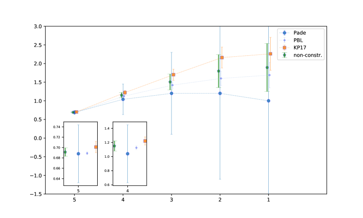
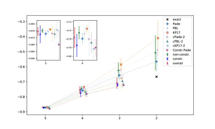
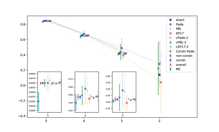
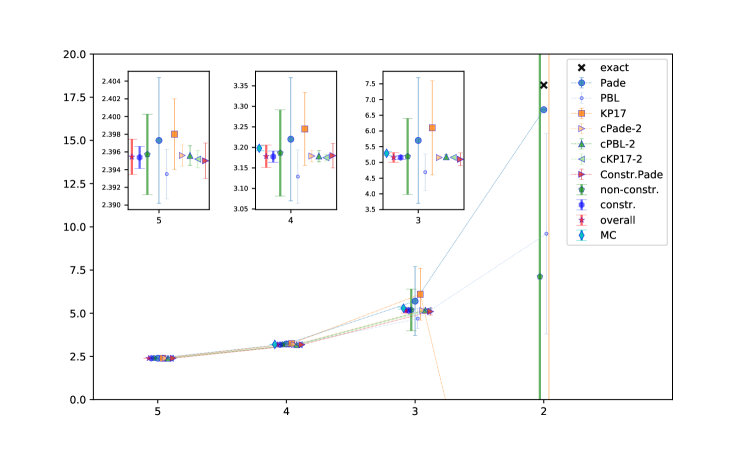
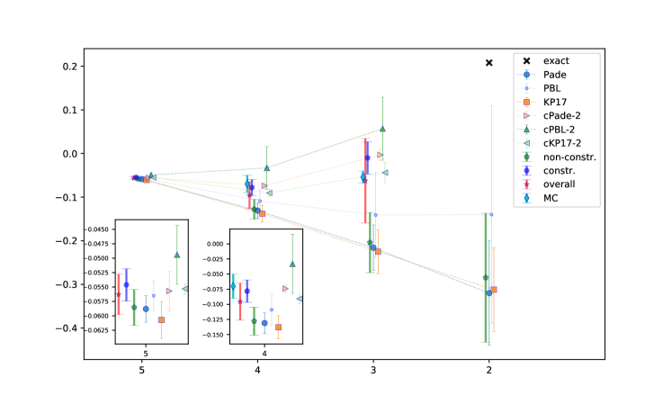
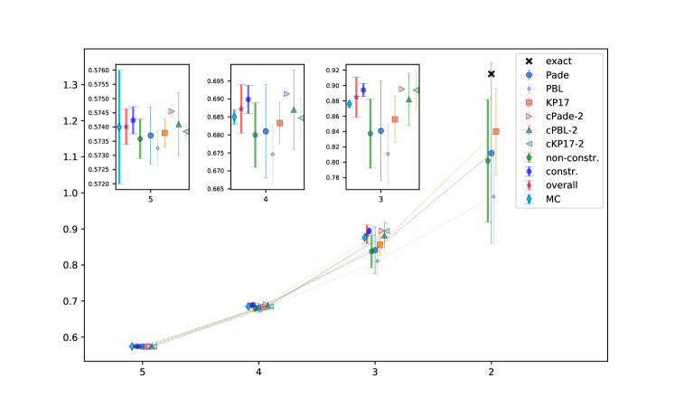
Having outlined the technical description of each of the resummation methods we have used to extract critical exponents as well as how we arrive at our error estimates, we devote this section to recording the actual values for a wide range of exponents. For both Lee–Yang edge singularity and percolation theory a table is provided for each exponent. In addition we illustrate that data with an associated figure. Each figure shows the exponent estimates with errors for dimensions 2, 3, 4 and 5 together with our overall Monte Carlo summary values where these are available. The horizontal axis in each figure corresponds to dimension .
6.1 Lee–Yang edge singularity
For our Lee–Yang singularity analysis we focus on a small set of exponents. As the main work of others has centred primarily around the exponent we have compiled as comprehensive an amount of independent results as possible in order to draw comparisons. For and , aside from the three loop work of [5], we were only able to find one study of these exponents which was [11]. That used the functional renormalization group approach and determined and directly. An additional exponent termed was also computed. From the hyperscaling relations given in [11], it can be related to our and via the expression . We have used the values for and of [11] to produce an independent estimate for to benchmark our results against. Each of the tables follows a common theme. The top part of each is a compilation of data from numerical methods with sources. This is followed by our resummation analysis for both four and five loops. The former is provided to gauge convergence. In each case three lines summarize the unconstrained and constrained estimates as well as the combination of both. This can be compared to a similar estimate from Monte Carlo (MC) and series (srs) data.
| Reference | ||||||
|---|---|---|---|---|---|---|
| exact | -1.0 | -0.8 | ||||
| MC/ srs | [11] (2016) | -0.586(29) | -0.316(16) | -0.126(6) | ||
| overall | -0.586(29) | -0.316(16) | -0.126(6) | |||
| 4 loops | Padé | -1.177 | -0.8655 | -0.5893 | -0.38(11) | -0.153(12) |
| KP17 | -1.2(9) | -0.9(5) | -0.6(3) | -0.45(10) | -0.161(8) | |
| cPadé-1 | -0.77(4) | -0.55(4) | -0.34(2) | -0.149(4) | ||
| cPadé-2 | -0.56(2) | -0.344(15) | -0.149(4) | |||
| cPBL-1 | -0.78(2) | -0.56(3) | -0.345(14) | -0.150(3) | ||
| cPBL-2 | -0.570(13) | -0.349(10) | -0.151(2) | |||
| cKP17-1 | -0.763(8) | -0.539(11) | -0.332(9) | -0.147(3) | ||
| cKP17-2 | -0.556(9) | -0.338(8) | -0.148(3) | |||
| Constr. Padé | -0.581(11) | -0.356(10) | -0.152(3) | |||
| non constr. | -1.2(9) | -0.9(5) | -0.6(3) | -0.42(11) | -0.158(10) | |
| constr. | -0.77(2) | -0.56(2) | -0.343(14) | -0.149(3) | ||
| all | -1.2(9) | -0.77(3) | -0.56(2) | -0.35(2) | -0.150(5) | |
| 5 loops | Padé | -1.249 | -0.9148 | -0.6185 | -0.39(9) | -0.154(7) |
| PBL | -0.9(5) | -0.8(3) | -0.55(12) | -0.34(4) | -0.150(3) | |
| KP17 | -1.2(2) | -0.91(11) | -0.61(4) | -0.36(7) | -0.152(11) | |
| cPadé-1 | -0.78(3) | -0.56(2) | -0.346(11) | -0.151(2) | ||
| cPadé-2 | -0.570(13) | -0.349(8) | -0.1509(14) | |||
| cPBL-1 | -0.785(11) | -0.564(11) | -0.348(6) | -0.1508(11) | ||
| cPBL-2 | -0.571(6) | -0.350(4) | -0.1511(8) | |||
| cKP17-1 | -0.765(7) | -0.542(9) | -0.334(8) | -0.148(4) | ||
| cKP17-2 | -0.557(9) | -0.338(8) | -0.148(3) | |||
| Constr. Padé | -0.580(7) | -0.356(6) | -0.1521(13) | |||
| non constr. | -1.2(3) | -0.9(2) | -0.60(7) | -0.36(6) | -0.152(6) | |
| constr. | -0.774(15) | -0.565(15) | -0.347(10) | -0.151(2) | ||
| all | -1.2(3) | -0.78(3) | -0.57(2) | -0.347(12) | -0.151(2) |
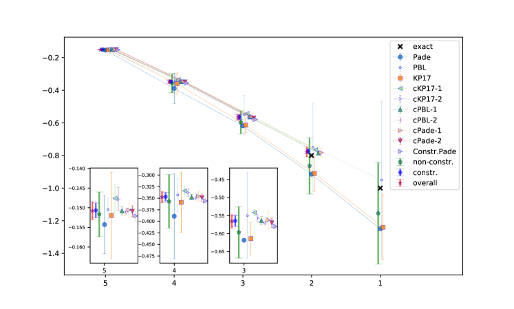
For the exponent our results are in Table 1. We see that the estimates for the three key dimensions are stable from four to five loops. However for the only available study that we could locate [11] there is some overlap agreement for the 3 dimensional estimate in contrast to those for higher dimensions. Although this exponent is ordinarily regarded as one of the more difficult ones to reconcile between different methods since it is very close to zero. This is not the case here.
| Reference | ||||||
|---|---|---|---|---|---|---|
| MC/ srs | [11] (2016) | (4.826146) | (1.187477) | (0.696008) | ||
| overall | ||||||
| 4 loops | Padé | 1.088 | 0.701(4) | |||
| KP17 | 1.6(1.2) | 1.3(9) | 1.1(6) | 0.9(3) | 0.69(3) | |
| non constr. | 1.6(1.2) | 1.3(9) | 1.1(6) | 0.9(3) | 0.699(8) | |
| all | 1.6(1.2) | 1.3(9) | 1.1(6) | 0.9(3) | 0.699(8) | |
| 5 loops | Padé | 0.7022(12) | ||||
| PBL | 2(2) | 1.6(1.2) | 1.3(5) | 0.98(10) | 0.696(3) | |
| KP17 | 1.6(1.3) | 1.4(1.0) | 1.1(7) | 0.9(2) | 0.70(2) | |
| non constr. | 2(2) | 1.5(1.1) | 1.2(6) | 0.95(14) | 0.700(4) | |
| all | 2(2) | 1.5(1.1) | 1.2(6) | 0.95(14) | 0.700(4) |
| Reference | ||||||
|---|---|---|---|---|---|---|
| exact | -1.0 | -2.5 | ||||
| MC/ srs | [11] (2016) | (4.826146) | (1.187477) | (0.696008) | ||
| overall | ||||||
| 4 loops | Padé | -1.1(1.1) | -3(5) | 4(3) | 1.18(10) | 0.701(4) |
| PBL | -1(2) | -4(11) | 3(3) | 1.17(14) | 0.700(6) | |
| KP17 | -0.8(3) | -2.1(1.1) | 6(4) | 1.23(5) | 0.702(3) | |
| cPadé-1 | -2.58(11) | 4.5(3) | 1.205(14) | 0.7015(10) | ||
| cPadé-2 | 4.6(2) | 1.208(10) | 0.7016(8) | |||
| cPBL-1 | -2.56(8) | 4.5(3) | 1.208(10) | 0.7017(6) | ||
| cPBL-2 | 4.64(14) | 1.211(7) | 0.7019(5) | |||
| cKP17-1 | -2.61(7) | 4.4(3) | 1.20(2) | 0.701(2) | ||
| cKP17-2 | 4.58(12) | 1.206(8) | 0.7017(11) | |||
| Constr. Padé | 4.74(2) | 1.215(2) | 0.7022(2) | |||
| non constr. | -1.0(7) | -2(3) | 4(3) | 1.20(9) | 0.701(4) | |
| constr. | -2.58(9) | 4.67(13) | 1.211(8) | 0.7019(6) | ||
| all | -1.0(7) | -2.6(2) | 4.7(2) | 1.211(11) | 0.7019(9) | |
| 5 loops | Padé | -1.0(4) | -2.4(1.3) | 5(2) | 1.22(4) | 0.7022(12) |
| PBL | -2(2) | -5(11) | 3(2) | 1.17(8) | 0.701(2) | |
| KP17 | -0.92(15) | -2.3(5) | 5.0(1.2) | 1.22(2) | 0.7021(11) | |
| cPadé-1 | -2.55(8) | 4.6(2) | 1.209(8) | 0.7019(4) | ||
| cPadé-2 | 4.65(14) | 1.211(6) | 0.7020(3) | |||
| cPBL-1 | -2.54(4) | 4.60(11) | 1.210(4) | 0.7019(2) | ||
| cPBL-2 | 4.66(6) | 1.212(2) | 0.70199(14) | |||
| cKP17-1 | -2.61(9) | 4.4(3) | 1.211(15) | 0.7020(5) | ||
| cKP17-2 | 4.58(14) | 1.212(10) | 0.7020(7) | |||
| Constr. Padé | 4.71(7) | 1.214(4) | 0.7021(2) | |||
| non constr. | -1.0(3) | -2.4(1.2) | 4(2) | 1.21(4) | 0.7019(14) | |
| constr. | -2.56(6) | 4.61(14) | 1.211(5) | 0.7020(3) | ||
| all | -1.0(3) | -2.6(2) | 4.6(2) | 1.211(8) | 0.7020(4) |
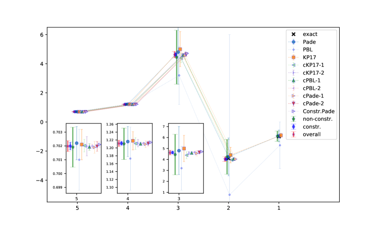
Our direct estimate of suffered from singularity issues. To illustrate this situation we have included Table 2 where data from those few techniques that did render a reliable estimate are presented. However the resultant large error bars mean that these values cannot be regarded as reliable. Instead we took a different tack and applied our resummation to the series for before inverting the final numerical value. This gave problem-free data for all our approaches which is recorded in Table 3. The behaviour of over the dimensions indicates that there is a maximum. Clearly is positive and increases as decreases to a large value in dimensions before becoming negative in two dimensions where the exact values are known. The functional renormalization group results have a similar behaviour and we are in qualitative accord at the very least.
| Reference | ||||||
|---|---|---|---|---|---|---|
| exact | -0.5 | -0.1667 | ||||
| MC/srs | [5] (1981) | -0.146 – -0.166 | 0.079–0.091 | 0.262–0.266 | 0.399–0.400 | |
| [76] (1995) | -0.165(6) | 0.080(6) | 0.261(12) | 0.40(2) | ||
| (hdsc) [26] (2012) | -0.1662(5) | 0.077(2) | 0.258(5) | 0.401(9) | ||
| (hdbcc) [26] (2012) | -0.1662(5) | 0.076(2) | 0.261(4) | 0.402(2) | ||
| [77] (2014) | -0.161(8) | 0.0877(25) | 0.2648(16) | 0.402(5) | ||
| [10] (2014) | -0.1664(5) | 0.085(1) | 0.2685(1) | 0.4105(5) | ||
| [11] (2016) | 0.0742(56) | 0.2667(32) | 0.4033(12) | |||
| (FRG) [12] (2017) | 0.2648(6) | 0.40166(2) | ||||
| (LPA) [12] (2017) | -0.193 | 0.0588 | 0.245 | 0.394 | ||
| overall | -0.1661(11) | 0.081(5) | 0.267(2) | 0.402(2)/0.407(4) | ||
| 4 loops | Padé | -0.1(4) | 0.0(2) | 0.16(12) | 0.27(4) | 0.400(4) |
| PBL | -0.1(4) | 0.0(2) | 0.16(12) | 0.28(4) | 0.401(4) | |
| KP17 | 0.1(6) | -0.3(4) | 0.0(2) | 0.24(2) | 0.397(3) | |
| cPadé-1 | -0.18(2) | 0.07(2) | 0.258(7) | 0.3983(12) | ||
| cPadé-2 | 0.073(10) | 0.259(6) | 0.3983(10) | |||
| cKP17-1 | -0.17(3) | 0.07(3) | 0.258(11) | 0.398(2) | ||
| cKP17-2 | 0.074(12) | 0.258(8) | 0.398(2) | |||
| Constr. Padé | 0.077(2) | 0.260(2) | 0.3985(5) | |||
| non constr. | -0.1(5) | -0.1(3) | 0.1(2) | 0.26(4) | 0.399(4) | |
| constr. | -0.18(3) | 0.075(7) | 0.259(5) | 0.3984(7) | ||
| all | -0.1(5) | -0.16(9) | 0.08(2) | 0.259(9) | 0.3985(11) | |
| 5 loops | Padé | -0.3113 | -0.0923 | 0.1002 | 0.26(3) | 0.398(2) |
| PBL | -0.2(2) | -0.02(12) | 0.13(5) | 0.272(13) | 0.3991(8) | |
| KP17 | -0.21(10) | 0.06(6) | 0.257(14) | 0.3982(12) | ||
| cPadé-1 | -0.18(2) | 0.068(12) | 0.257(4) | 0.3983(8) | ||
| cPadé-2 | 0.072(6) | 0.258(3) | 0.3981(4) | |||
| cPBL-1 | -0.18(3) | 0.07(2) | 0.257(7) | 0.3981(7) | ||
| cPBL-2 | 0.072(11) | 0.258(5) | 0.3981(6) | |||
| cKP17-1 | -0.17(2) | 0.072(12) | 0.258(4) | 0.3983(5) | ||
| cKP17-2 | 0.075(6) | 0.259(2) | 0.3984(4) | |||
| Constr. Padé | 0.078(2) | 0.2602(14) | 0.3984(2) | |||
| non constr. | -0.2(2) | -0.12(14) | 0.10(6) | 0.26(2) | 0.3986(13) | |
| constr. | -0.18(2) | 0.075(7) | 0.259(3) | 0.3983(5) | ||
| all | -0.2(2) | -0.17(5) | 0.075(11) | 0.259(5) | 0.3983(6) |
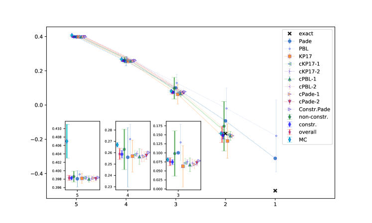
For a similar picture emerges in Table 4 where and indicate results in dimensions from separate simulations. Also FRG denotes the functional renormalization group and LPA indicates the use of the local potential approximation. In compiling the overall estimate and error for the first bank of the table we have excluded the results of [5] and the LPA data of [12] due to the absence of errors. We provide two estimates in 5 dimensions. The first includes the FRG result of [12] while the second omits it. Clearly with the increase in the order of the individual constrained estimates are in good agreement for and dimensions but less so for dimensions. This is primarily because the monotonic decrease in the value of from down to dimensions where it is positive in the critical dimension but negative in and means that at some non-integer dimension it will vanish. This appears to be in the neighbourhood of dimensions as indicated by the relatively small value in the hundredths. Indeed this is similar to the situation alluded to for in certain problems. Moreover the same feature is present in dimensional estimates from the other methods we have provided in Table 4. This is ultimately reflected in our final five loop estimate and in particular in the error. This should not overlook however the very good agreement for and dimensions.
One way of gauging the accuracy of our Lee–Yang exponents is to use them to provide exponent estimates in a related model. One such example is the lattice animal problem, reviewed in [78], which at criticality is related to the Lee–Yang edge singularity problem, [79]. In particular it was shown there that the Lee–Yang critical exponents in dimensions are the same as those of the lattice animal problem in dimensions. In [80] estimates were given for the exponents denoted by and by calculating general dimension series up to the th order. The relation these two exponents have to the Lee–Yang exponent studied here is [79],
| (54) |
With these we have compiled Table 5 which records our estimates for both exponents using our 5 loop cKP17-2 Lee–Yang values for . The table also records the summary results of Table VII of [80] for comparison. It is reassuring to note that our estimates are consistent with [80].
| this work | of [80] | this work | of [80] | |
|---|---|---|---|---|
| Reference | ||||||
|---|---|---|---|---|---|---|
| 4 loops | Padé | 1(4) | 1(3) | 1.3(1.4) | 1.1(5) | 0.69(10) |
| PBL | 2.4(5) | 2.1(3) | 1.7(2) | 1.22(6) | 0.704(11) | |
| KP17 | 2.3(6) | 1.9(4) | 1.6(3) | 1.18(14) | 0.69(3) | |
| non constr. | 2.3(8) | 2.0(5) | 1.6(3) | 1.20(13) | 0.70(2) | |
| all | 2.3(8) | 2.0(5) | 1.6(3) | 1.20(13) | 0.70(2) | |
| 5 loops | Padé | 1(4) | 1(2) | 1.2(1.1) | 1.0(4) | 0.69(6) |
| PBL | 1.7(3) | 1.6(2) | 1.42(8) | 1.12(3) | 0.689(3) | |
| KP17 | 2.3(4) | 2.2(3) | 1.70(15) | 1.22(6) | 0.701(11) | |
| non constr. | 1.9(6) | 1.8(4) | 1.5(2) | 1.15(7) | 0.691(8) | |
| all | 1.9(6) | 1.8(4) | 1.5(2) | 1.15(7) | 0.691(8) |
Finally the situation with the exponent is less clear. This is primarily due to the lack of an exact value for this exponent in two dimensions. Therefore we are only able to record the results of unconstrained resummations which are given in Table 6. Equally we were unable to compare the estimates with Monte Carlo studies. So no definite conclusions should be drawn for in the Lee–Yang study.
6.2 Percolation theory
For percolation theory we recall the exact two dimensional values of the various exponents in Table 7 that were used when constraints were implemented as indicated in Section 5. We will use the 2 dimensional estimate for the unconstrained resummations as a benchmark to gauge whether our extrapolation is consistent with the exact value. In several instances there was either a significant undershoot or overshoot for both the unconstrained and constrained case. This gave a strong indication that the higher dimensional estimates could be unreliable. Consequently we examined the expansion of various functions of the exponent, such as its reciprocal. Some of these gave improved estimates and a projection to 2 dimensions that was more in keeping with the exact values. This is illustrated in Table 7 which also summarizes our five loop two dimensional estimates from the various resummation methods. The table also records the summary of [27]; see also [81, Table 2]. While the exact values derive from two dimensional conformal field theory we note that a Monte Carlo study [82] which predated [25] gave estimates that were in remarkably good agreement. For instance, the values of , , , , and were determined in [82].
We note that here we use the value of for and for . This is in contrast with the value of for used in [18] based on [83] which also gave an argument that was . The discrepancy between the exact 2 dimensional values for and was discussed at length in [84]. In both cases the ratio is the same and corresponds to the fractal dimension of the system. Further a summary is given in [84] of independent calculations of both exponents. These appear to be more consistent with the respective exact values of and . One test is the value of the exponent which is for but for [83]. We note that naively taking our central values gives for .
| exponent | exact | numerical | 4 loop | 5 loop | |||
|---|---|---|---|---|---|---|---|
| overall | Padé | PBL | KP17 | overall | |||
| -0.667 | -0.56(9) | -0.57(6) | -0.49(13) | -0.41(12) | -0.51(11) | ||
| 0.139 | 0.2(3) | 0.3(3) | 0.3(3) | 0.04(40) | 0.2(3) | ||
| 2.39 | 1.9(4) | 2.0(4) | 1.8(3) | 2.2(3) | 2.0(4) | ||
| 18.2 | 4(2) | 3(5) | 4(2) | 4(3) | |||
| 7(15) | 16.78 | 10(6) | -25(75) | 7(14) | |||
| 0.208 | -0.32(11) | -0.32(12) | -0.1(2) | -0.31(10) | -0.28(15) | ||
| 1.33 | 0.87(15) | 0.9315 | 0.86(13) | 0.8(3) | 0.9(2) | ||
| 1.1(4) | 1.1(2) | 0.99(13) | 1.17(12) | 1.1(2) | |||
| 0.396 | 0.46(4) | 0.44(4) | 0.446(13) | 0.44(5) | 0.44(2) | ||
| 2.06 | 2.08(10) | 2.07(4) | 2.08(2) | 2.00(13) | 2.07(4) | ||
| 0.791 | 0.76(2) | 0.6(3) | 0.96(5) | 0.7(2) | 0.9(2) | ||
| 1.5 | 2.6(2) | 2(2) | 2.37(5) | 2.8(7) | 2.4(2) | ||
We now discuss the results for each exponent in alphabetical order. In Tables 8–19 we have summarized the estimates for the various exponents in the literature. One excellent source we benefited from in this respect is the table of [27] which is regularly updated. Included in this are our results for the various resummations. In several of our tables we also have a line designated as . This records the results of the constrained Padé method at four loops given in [18].
To open with, our estimates for are presented in Table 8. One aspect that is evident is the close agreement of the estimates from both the constrained and unconstrained approaches for both 4 and 5 dimensions and to a lesser extent for dimensions. The latter is in essence due to the overshoot of the two dimensional exact value for the unconstrained methods. Indeed the five loop value has a more pronounced discrepancy than at four loops. Given the slower decrease in the constrained estimate as decreases, we would take the position that those estimates are probably more reliable. Independent Monte Carlo data for each dimension would be useful to compare with.
| Reference | |||||
|---|---|---|---|---|---|
| exact | -0.6667 | ||||
| 4 loops | Padé | -0.58(6) | -0.67(4) | -0.76(2) | -0.873(3) |
| PBL | -0.57(6) | -0.66(4) | -0.76(2) | -0.872(3) | |
| KP17 | -0.46(15) | -0.60(7) | -0.74(3) | -0.869(4) | |
| cPadé-2 | -0.708(11) | -0.778(9) | -0.875(3) | ||
| cPBL-2 | -0.710(13) | -0.780(11) | -0.876(4) | ||
| cKP17-2 | -0.72(2) | -0.79(2) | -0.874(6) | ||
| Constr. Padé | -0.7212(4) | -0.782(14) | -0.877(5) | ||
| non constr. | -0.56(9) | -0.65(5) | -0.76(2) | -0.871(4) | |
| constr. | -0.720(3) | -0.781(13) | -0.876(4) | ||
| all | -0.56(9) | -0.719(12) | -0.77(2) | -0.874(5) | |
| 5 loops | Padé | -0.57(6) | -0.66(3) | -0.759(12) | -0.872(2) |
| PBL | -0.49(13) | -0.62(6) | -0.75(2) | -0.871(2) | |
| KP17 | -0.41(12) | -0.59(4) | -0.736(7) | -0.8690(6) | |
| cPadé-2 | -0.703(14) | -0.773(9) | -0.8739(13) | ||
| cPBL-2 | -0.69(4) | -0.77(2) | -0.872(4) | ||
| cKP17-2 | -0.72(2) | -0.78(2) | -0.870(6) | ||
| Constr. Padé | -0.723(2) | -0.78(2) | -0.880(10) | ||
| non constr. | -0.51(11) | -0.62(5) | -0.745(15) | -0.870(2) | |
| constr. | -0.720(11) | -0.77(3) | -0.873(6) | ||
| all | -0.51(11) | -0.71(3) | -0.76(2) | -0.870(3) |
For the situation is much clearer in that we have several independent results provided in Table 9. Again there is a large degree of stability within each of the comparable methods and loop order although the unconstrained Padé clearly overshoots the two dimensional exact result. From four to five loops the final estimates are remarkably stable. Comparing, however, with [85, 86] the loop estimates are all slightly larger even for 5 dimensions.
| Reference | |||||
|---|---|---|---|---|---|
| exact | 0.1389 | ||||
| [18] (2015) | 0.4273 | 0.6590 | 0.8457 | ||
| MC/srs | [86] (1976) | 0.41(1) | |||
| [85] (1990) | 0.405(25) | 0.639(20) | 0.835(5) | ||
| overall | 0.409(14) | 0.64(2) | 0.835(5) | ||
| 4 loops | Padé | 0.3(3) | 0.49(13) | 0.68(4) | 0.847(4) |
| KP17 | 0.0(4) | 0.40(9) | 0.65(2) | 0.845(4) | |
| cPadé-2 | 0.426(8) | 0.657(5) | 0.8453(12) | ||
| cPBL-2 | 0.419(7) | 0.653(5) | 0.8444(12) | ||
| cKP17-2 | 0.424(11) | 0.656(7) | 0.845(2) | ||
| Constr. Padé | 0.4303 | 0.6599(2) | 0.8458 | ||
| non constr. | 0.2(3) | 0.43(11) | 0.66(3) | 0.846(4) | |
| constr. | 0.423(9) | 0.656(6) | 0.8449(14) | ||
| all | 0.2(3) | 0.42(2) | 0.656(10) | 0.845(2) | |
| 5 loops | Padé | 0.3(3) | 0.49(13) | 0.68(4) | 0.845(4) |
| PBL | 0.3(3) | 0.48(13) | 0.67(4) | 0.847(4) | |
| KP17 | 0.0(4) | 0.39(6) | 0.650(11) | 0.8447(10) | |
| cPadé-2 | 0.427(6) | 0.658(4) | 0.8455(6) | ||
| cPBL-2 | 0.417(5) | 0.653(2) | 0.8448(2) | ||
| cKP17-2 | 0.422(5) | 0.655(3) | 0.8450(5) | ||
| Constr. Padé | 0.42(2) | 0.656(12) | 0.8453(15) | ||
| non constr. | 0.2(3) | 0.44(10) | 0.66(2) | 0.845(2) | |
| constr. | 0.420(8) | 0.655(4) | 0.8449(5) | ||
| all | 0.2(3) | 0.42(2) | 0.655(7) | 0.8449(7) |
| Reference | |||||
|---|---|---|---|---|---|
| exact | 2.3889 | ||||
| [18] (2015) | 1.8357 | 1.4500 | 1.1817 | ||
| MC/srs | [86] (1976) | 1.6 | |||
| [85] (1990) | 1.805(20) | 1.435(15) | 1.185(5) | ||
| overall | 1.805(20) | 1.435(15) | 1.185(5) | ||
| 4 loops | Padé | 1.946 | 1.7(3) | 1.44(6) | 1.179(7) |
| PBL | 1.9(3) | 1.65(14) | 1.40(5) | 1.175(7) | |
| KP17 | 1.9(8) | 1.8(2) | 1.44(6) | 1.181(4) | |
| cPadé-2 | 1.83(3) | 1.45(2) | 1.181(3) | ||
| cKP17-2 | 1.82(6) | 1.44(4) | 1.180(6) | ||
| Constr. Padé | 1.82(4) | 1.44(2) | 1.180(3) | ||
| non constr. | 1.9(4) | 1.7(2) | 1.42(6) | 1.179(6) | |
| constr. | 1.82(4) | 1.44(2) | 1.180(4) | ||
| all | 1.9(4) | 1.81(8) | 1.44(3) | 1.180(5) | |
| 5 loops | Padé | 2.0(4) | 1.8(2) | 1.45(4) | 1.181(4) |
| PBL | 1.8(3) | 1.6(2) | 1.38(4) | 1.176(3) | |
| KP17 | 2.2(3) | 1.77(13) | 1.43(2) | 1.179(2) | |
| cPadé-2 | 1.83(3) | 1.448(13) | 1.181(2) | ||
| cPBL-2 | 1.83(4) | 1.45(2) | 1.181(3) | ||
| cKP17-2 | 1.81(5) | 1.437(13) | 1.1797(14) | ||
| Constr. Padé | 1.83(3) | 1.444(14) | 1.181(2) | ||
| non constr. | 2.0(4) | 1.7(2) | 1.42(4) | 1.179(3) | |
| constr. | 1.82(4) | 1.44(2) | 1.180(2) | ||
| all | 2.0(4) | 1.81(8) | 1.44(3) | 1.180(3) |
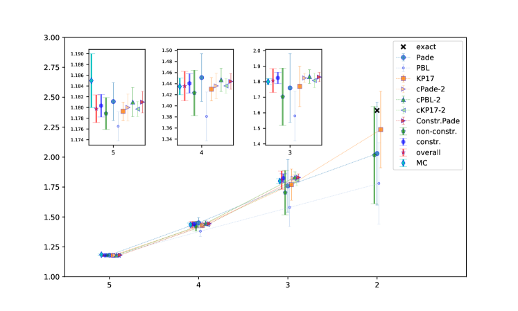
In the case of the independent Monte Carlo data was only available from the same articles as our comparison for . There was a similar picture for our estimates in that there was remarkable stability between four and five loops for the three dimensions of interest as is clear from Table 10. However the check estimate for two dimensions was much closer to the exact value than that for . This may be one of the reasons why our final values for five loops are in remarkably good agreement with the Monte Carlo results of [85]. There was no error bar for the 3 dimensional result of [86]. So it is not clear how to interpret the central value that is 12% lower than both [85] and our estimate at five loops.
| Reference | |||||
|---|---|---|---|---|---|
| exact | 18.2 | ||||
| MC/srs | [86] (1976) | 3.198(6) | |||
| [87] (1980) | 5.3 | 3.9 | 3.0 | ||
| [88] (1998) | 5.29(6) | ||||
| overall | 5.29(6) | 3.198(6) | |||
| 4 loops | Padé | 4.756 | 3.742 | 3.1(2) | 2.391(14) |
| KP17 | 4(2) | 3.3(1.3) | 3.1(4) | 2.39(3) | |
| cPadé-2 | 7.831 | 3.2(3) | 2.40(2) | ||
| cPBL-2 | 11(4) | 6(4) | 2.6(4) | ||
| cKP17-2 | 10(4) | 3(2) | 2.40(11) | ||
| Constr. Padé | 5.1(2) | 3.15(5) | 2.393(5) | ||
| non constr. | 4(2) | 3.3(1.3) | 3.1(3) | 2.39(2) | |
| constr. | 6(2) | 3.2(3) | 2.40(2) | ||
| all | 4(2) | 5(2) | 3.2(3) | 2.40(2) | |
| 5 loops | Padé | 3.15(8) | 2.396(5) | ||
| PBL | 3(5) | 3(3) | 2.5(1.5) | 2.3(2) | |
| KP17 | 4(2) | 3.3(1.5) | 3.2(2) | 2.396(6) | |
| cPadé-2 | 7.831 | 3.3(3) | 2.40(2) | ||
| cPBL-2 | 8.92(5) | 3.84(2) | 2.4061(12) | ||
| cKP17-2 | 10(4) | 3.3(1.3) | 2.40(5) | ||
| Constr. Padé | 5.16(7) | 3.175(14) | 2.3954(11) | ||
| non constr. | 4(3) | 3(2) | 3.1(2) | 2.395(12) | |
| constr. | 7(2) | 3.4(3) | 2.401(6) | ||
| overall | 4(3) | 7(2) | 3.4(3) | 2.400(7) |
The situation with was much less straightforward and we include two tables with data. In Table 11 we have applied our various resummation techniques directly to the expansion of . This illustrates one immediate difficulty in obtaining reliable values for low . The value for in exactly 6 dimensions is whereas it is exactly in two dimensions. The latter places a big restriction on the ability of the expansion to manufacture large corrections as decreases. This is clear in both our four and five loop estimates from both our unconstrained and constrained resummations. Moreover the skew that is necessary to meet the two dimensional constraint clearly makes the convergence between loops in 3 dimensions impossible. Equally there is no agreement with the few independent estimates which both have more precise values. Although the direct expansion approach is problematic we have provided it here partly to be transparent in the application of our methods but also to highlight the hidden pitfalls in naively applying various resummation methods. Equally to address this problem we have instead tried a second approach which was to sum the expansion of , determine a numerical value and then invert this. The results of this exercise are given in Table 12. Many of the failings with the direct evaluation are absent now. There is a degree of stability between the various four and five loop results especially in 3 dimensions. Equally and more importantly we find that this and the 4 dimensional results are certainly not out of line with the results of [88, 86] although our 3 dimensional result has large errors. While the extrapolation to 2 dimensions has larger errors it does accommodate the exact value. In some sense this much more consistent agreement across Table 12 is an a posteriori justification of following this second strategy.
| Reference | |||||
|---|---|---|---|---|---|
| exact | 18.2 | ||||
| MC/srs | [86] (1976) | 3.198(6) | |||
| [87] (1980) | 5.3 | 3.9 | 3.0 | ||
| [88] (1998) | 5.29(6) | ||||
| overall | 5.29(6) | 3.198(6) | |||
| 4 loops | Padé | 8(10) | 5(2) | 3.1(2) | 2.391(14) |
| PBL | 8(10) | 4.4(1.4) | 3.1(2) | 2.39(2) | |
| KP17 | -20(120) | 6.3(1.5) | 3.25(9) | 2.399(4) | |
| cPadé-2 | 5.13(11) | 3.17(3) | 2.395(3) | ||
| cPBL-2 | 5.19(8) | 3.18(2) | 2.396(2) | ||
| cKP17-2 | 5.15(12) | 3.17(3) | 2.395(5) | ||
| Constr. Padé | 5.2(2) | 3.17(6) | 2.394(6) | ||
| non constr. | 7(15) | 5(2) | 3.2(2) | 2.395(9) | |
| constr. | 5.17(12) | 3.18(3) | 2.395(3) | ||
| all | 7(15) | 5.2(3) | 3.18(5) | 2.395(5) | |
| 5 loops | Padé | 16.78 | 6(2) | 3.22(15) | 2.397(7) |
| PBL | 10(6) | 4.7(6) | 3.13(7) | 2.393(3) | |
| KP17 | -25(75) | 6.1(1.5) | 3.25(9) | 2.398(4) | |
| cPadé-2 | 5.16(5) | 3.179(14) | 2.3956(12) | ||
| cPBL-2 | 5.18(7) | 3.179(14) | 2.3956(11) | ||
| cKP17-2 | 5.16(3) | 3.175(8) | 2.3952(10) | ||
| Constr. Padé | 5.1(2) | 3.17(3) | 2.395(2) | ||
| non constr. | 7(14) | 5.2(1.2) | 3.19(11) | 2.396(5) | |
| constr. | 5.16(6) | 3.176(14) | 2.3954(12) | ||
| all | 7(14) | 5.16(15) | 3.18(3) | 2.396(2) |
| Reference | |||||
|---|---|---|---|---|---|
| exact | 0.2083 | ||||
| [18] (2015) | -0.0470 | -0.0954 | -0.0565 | ||
| MC/srs | [85] (1990) | -0.07(5) | -0.12(4) | -0.075(20) | |
| [89] (1996) | -0.0944(28) | ||||
| [88] (1998) | -0.046(8) | ||||
| [90] (1998) | -0.059(9) | ||||
| [91] (2001) | -0.0929(9) | ||||
| overall | -0.054(14) | -0.094(4) | -0.075(20) | ||
| 4 loops | Padé | -0.32(13) | -0.21(6) | -0.13(2) | -0.059(3) |
| KP17 | -0.33(10) | -0.23(5) | -0.14(2) | -0.061(3) | |
| cPadé-2 | 0.01143 | -0.06287 | -0.055(7) | ||
| cPBL-2 | 0.04(9) | -0.06(3) | -0.051(6) | ||
| cKP17-2 | -0.09(12) | -0.10(3) | -0.057(3) | ||
| non constr. | -0.32(11) | -0.22(5) | -0.13(2) | -0.060(3) | |
| constr. | -0.02(12) | -0.08(4) | -0.055(5) | ||
| all | -0.32(11) | -0.15(13) | -0.12(4) | -0.057(5) | |
| 5 loops | Padé | -0.32(12) | -0.22(5) | -0.13(2) | -0.059(2) |
| PBL | -0.1(2) | -0.14(10) | -0.11(3) | -0.057(3) | |
| KP17 | -0.31(10) | -0.23(5) | -0.14(2) | -0.061(3) | |
| cPadé-2 | -0.003(13) | -0.074(7) | -0.056(4) | ||
| cPBL-2 | 0.06(7) | -0.03(5) | -0.049(5) | ||
| cKP17-2 | -0.04(2) | -0.091(8) | -0.0553(9) | ||
| Scaling Padé | (-0.0566) | (-0.0833) | (-0.0545) | ||
| Hyperscaling Padé | (-0.0176) | (-0.0790) | (-0.0540) | ||
| non constr. | -0.28(15) | -0.20(7) | -0.13(2) | -0.059(3) | |
| constr. | -0.01(4) | -0.08(2) | -0.055(3) | ||
| all | -0.28(15) | -0.06(10) | -0.10(3) | -0.056(3) |
We now turn to one of the more widely measured exponents which is with data recorded in Table 13. As is the case with in other problems its value in percolation is relatively small and close to zero being associated with the wave function anomalous dimension. Consequently it is difficult to obtain an accurate value for it that is in consistent agreement with other estimates. This is evident in the numerical values of [85, 88, 90, 91, 89] in 3 and 4 dimensions although those of [91, 89] are the most accurate and do overlap. On the expansion side the Padé resummations suffered from the presence of at least one singularity in or were not monotonic. For this case we indirectly estimated using the respective scaling and hyperscaling relations
| (55) |
The numerical values for each of these are bracketed to indicate that they were not derived directly. A more difficult issue to circumvent for in the constrained approach is the relatively large and positive exact value in 2 dimensions. This means that would have to be identically zero somewhere between and dimensions as decreases. So while our final 3 dimensional estimate of has shown an improvement from four to five loops this is to be balanced against a necessarily large error.
| Reference | |||||
|---|---|---|---|---|---|
| exact | 1.3333 | ||||
| [18] (2015) | 0.8960 | 0.6920 | 0.5746 | ||
| MC/srs | [92] (1975) | 0.80(5) | |||
| [86] (1976) | 0.8(1) | ||||
| [85] (1990) | 0.872(70) | 0.678(50) | 0.571(3) | ||
| [89] (1997) | 0.689(10) | ||||
| [88] (1998) | 0.875(1) | ||||
| [93] (2000) | 0.8765(18) | ||||
| [94] (2013) | 0.8764(12) | ||||
| [95] (2014) | 0.8751(11) | ||||
| [96] (2014) | 0.87619(11) | ||||
| [97] (2016) | 0.8774(13) | 0.6852(28) | 0.5723(18) | ||
| [13] (2018) | 0.693 | ||||
| [98] (2020) | 0.6845(6) | 0.5757(7) | |||
| overall | 0.876(4) | 0.685(2) | 0.574(2) | ||
| 4 loops | Padé | 0.8812 | 0.78(8) | 0.68(2) | 0.573(2) |
| PBL | 0.88(10) | 0.77(5) | 0.66(2) | 0.572(3) | |
| KP17 | 0.8(3) | 0.9(2) | 0.68(3) | 0.574(3) | |
| cPadé-2 | 0.9496 | 0.697(15) | 0.575(2) | ||
| cKP17-2 | 0.95(12) | 0.69(4) | 0.574(3) | ||
| Constr. Padé | 0.896(3) | 0.6916(12) | 0.5746(2) | ||
| non constr. | 0.87(15) | 0.79(9) | 0.67(2) | 0.573(3) | |
| constr. | 0.897(10) | 0.692(4) | 0.5746(5) | ||
| all | 0.87(15) | 0.89(4) | 0.690(9) | 0.5744(11) | |
| 5 loops | Padé | 0.9315 | 0.81(5) | 0.681(13) | 0.5737(10) |
| PBL | 0.86(13) | 0.78(4) | 0.669(6) | 0.5730(2) | |
| KP17 | 0.8(3) | 0.85(8) | 0.682(11) | 0.5737(7) | |
| cPadé-2 | 0.9496 | 0.697(15) | 0.575(2) | ||
| cPBL-2 | 0.93(3) | 0.703(14) | 0.575(2) | ||
| cKP17-2 | 0.88(7) | 0.69(2) | 0.5738(12) | ||
| Constr. Padé | 0.89(2) | 0.689(6) | 0.5743(7) | ||
| non constr. | 0.9(2) | 0.80(6) | 0.675(11) | 0.5732(5) | |
| constr. | 0.90(4) | 0.692(13) | 0.563(13) | ||
| all | 0.9(2) | 0.87(7) | 0.685(15) | 0.570(9) |
The situation for is similar as can be seen in Tables 14 and 15 where we note that there has been a significant number of independent measurements of especially in dimensions. This has provided us with a very reliable benchmark to compare with. Again we had to apply our resummation methods to both and since the estimate of the former undershot the exact 2 dimensional value. This was not the case for the latter which we would regard as our results for . From Table 15 it is clear that our 4 and 5 dimensional five loop estimates are in very good accord with the Monte Carlo values and are an improvement on the four loop ones. The situation for 3 dimensions is good and also closer to numerical values.
| Reference | |||||
|---|---|---|---|---|---|
| exact | 1.3333 | ||||
| [18] (2015) | 0.8960 | 0.6920 | 0.5746 | ||
| MC/srs | [92] (1975) | 0.80(5) | |||
| [86] (1976) | 0.8(1) | ||||
| [85] (1990) | 0.872(70) | 0.678(50) | 0.571(3) | ||
| [89] (1997) | 0.689(10) | ||||
| [88] (1998) | 0.875(1) | ||||
| [93] (2000) | 0.8765(18) | ||||
| [94] (2013) | 0.8764(12) | ||||
| [95] (2014) | 0.8751(11) | ||||
| [96] (2014) | 0.87619(11) | ||||
| [97] (2016) | 0.8774(13) | 0.6852(28) | 0.5723(18) | ||
| [13] (2018) | 0.693 | ||||
| [98] (2020) | 0.6845(6) | 0.5757(7) | |||
| overall | 0.876(4) | 0.685(2) | 0.574(2) | ||
| 4 loops | Padé | 1.1(3) | 0.82(9) | 0.68(2) | 0.573(3) |
| PBL | 1.0(3) | 0.80(9) | 0.67(2) | 0.572(3) | |
| KP17 | 1.5(7) | 0.91(10) | 0.69(2) | 0.574(2) | |
| cPadé-2 | 0.896(3) | 0.6916(12) | 0.5746(2) | ||
| cPBL-2 | 0.896(2) | 0.6918(11) | 0.5746(2) | ||
| cKP17-2 | 0.90(3) | 0.685(10) | 0.5739(9) | ||
| Constr. Padé | 0.895(5) | 0.691(2) | 0.5745(3) | ||
| non constr. | 1.1(4) | 0.84(10) | 0.68(2) | 0.573(2) | |
| constr. | 0.896(4) | 0.691(2) | 0.5745(3) | ||
| all | 1.1(4) | 0.894(14) | 0.691(5) | 0.5744(7) | |
| 5 loops | Padé | 1.1(2) | 0.84(7) | 0.681(13) | 0.5737(10) |
| PBL | 0.99(13) | 0.81(4) | 0.675(8) | 0.5733(6) | |
| KP17 | 1.17(12) | 0.86(3) | 0.683(6) | 0.5738(5) | |
| cPadé-2 | 0.895(3) | 0.6914(13) | 0.5746(2) | ||
| cPBL-2 | 0.88(3) | 0.687(11) | 0.5741(11) | ||
| cKP17-2 | 0.89(3) | 0.685(5) | 0.5738(3) | ||
| Constr. Padé | 0.899(11) | 0.6913(12) | 0.5744(5) | ||
| non constr. | 1.1(2) | 0.84(5) | 0.680(9) | 0.5736(7) | |
| constr. | 0.894(9) | 0.690(3) | 0.5743(5) | ||
| all | 1.1(2) | 0.89(3) | 0.689(5) | 0.5741(6) |
| Reference | |||||
|---|---|---|---|---|---|
| exact | 0.3956 | ||||
| [18] (2015) | 0.4419 | 0.4642 | 0.4933 | ||
| MC/srs | [99] (1976) | 0.42(6) | |||
| [89] (1996) | 0.4522(8) | ||||
| [88] (1998) | 0.445(10) | ||||
| [96] (2014) | 0.45237(8) | ||||
| overall | 0.4523(13) | ||||
| 4 loops | Padé | 0.45(5) | 0.47(3) | 0.483(10) | 0.494(2) |
| PBL | 0.45(3) | 0.470(14) | 0.484(5) | 0.4946(10) | |
| KP17 | 0.47(6) | 0.48(4) | 0.475(13) | 0.4937(13) | |
| cPadé-2 | 0.442(2) | 0.476(6) | 0.4934(10) | ||
| cPBL-2 | 0.440(6) | 0.473(3) | 0.4930(5) | ||
| cKP17-2 | 0.448(9) | 0.478(5) | 0.4939(7) | ||
| Constr. Padé | 0.444(11) | 0.475(6) | 0.4932(13) | ||
| non constr. | 0.46(4) | 0.47(2) | 0.482(9) | 0.4943(13) | |
| constr. | 0.443(6) | 0.475(5) | 0.4934(8) | ||
| all | 0.46(4) | 0.447(13) | 0.477(7) | 0.4937(11) | |
| 5 loops | Padé | 0.44(4) | 0.46(2) | 0.480(6) | 0.4940(8) |
| PBL | 0.446(13) | 0.465(5) | 0.4814(15) | 0.49409(14) | |
| KP17 | 0.44(5) | 0.45(2) | 0.478(4) | 0.4939(3) | |
| cPadé-2 | 0.4425 | 0.476(6) | 0.4934(7) | ||
| cPBL-2 | 0.443(15) | 0.475(9) | 0.4935(11) | ||
| cKP17-2 | 0.452(7) | 0.4789(14) | 0.49396(13) | ||
| Constr. Padé | 0.447(9) | 0.477(5) | 0.4937(8) | ||
| non constr. | 0.44(2) | 0.462(12) | 0.480(3) | 0.4940(3) | |
| constr. | 0.448(12) | 0.478(4) | 0.4939(4) | ||
| overall | 0.44(2) | 0.454(14) | 0.479(4) | 0.4940(3) |

Examining Table 16 which summarizes our investigation for , we note that the only independent estimates are in dimensions. We have clearly obtained excellent agreement with these which exceed the situation with other exponents. This outcome has to be qualified by noting that in strictly 6 dimensions is with the exact result in 2 dimensions being just under . In other words the behaviour of in the intervening dimensions is a shallow decrease as decreases which underpins the very good overlap. Consequently even though there have been no measurements of in 4 and 5 dimensions that we can compare with, we would expect our five loop estimates to be in line with any future Monte Carlo studies in those dimensions.
| Reference | |||||
|---|---|---|---|---|---|
| exact | 2.0549 | ||||
| [18] (2015) | 2.1888 | 2.3124 | 2.4171 | ||
| MC/srs | [87] (1980) | 2.26 | 2.33 | ||
| [89] (1996) | 2.18906(8) | 2.3127(6) | |||
| [90] (1998) | 2.186(2) | ||||
| [88] (1998) | 2.189(2) | ||||
| [100] (2001) | 2.313(3) | 2.412(4) | |||
| [91] (2001) | 2.190(2) | 2.313(2) | |||
| [101] (2006) | 2.189(1) | ||||
| [96] (2014) | 2.18909(5) | ||||
| (site) [102] (2018) | 2.1892(1) | 2.3142(5) | 2.419(1) | ||
| (bond) [102] (2018) | 2.1890(2) | 2.311(2) | 2.422(4) | ||
| [103] (2019) | 2.3135(5) | ||||
| overall | 2.1891(4) | 2.3133(12) | 2.418(4) | ||
| 4 loops | Padé | 2.10(7) | 2.20(5) | 2.318(13) | 2.4180(15) |
| PBL | 2.11(7) | 2.22(3) | 2.323(10) | 2.4186(14) | |
| KP17 | 1.9(2) | 2.16(11) | 2.31(2) | 2.417(2) | |
| cPadé-2 | 2.195(4) | 2.315(3) | 2.4176(5) | ||
| cPBL-2 | 2.193(3) | 2.314(2) | 2.4174(3) | ||
| cKP17-2 | 2.194(4) | 2.315(3) | 2.4175(9) | ||
| Constr. Padé | 2.197(9) | 2.317(6) | 2.4179(10) | ||
| non constr. | 2.08(10) | 2.20(5) | 2.318(14) | 2.418(2) | |
| constr. | 2.194(5) | 2.315(3) | 2.4176(6) | ||
| all | 2.08(10) | 2.194(9) | 2.315(5) | 2.4176(8) | |
| 5 loops | Padé | 2.07(4) | 2.19(3) | 2.314(8) | 2.4174(7) |
| PBL | 2.08(2) | 2.202(8) | 2.317(2) | 2.4176(2) | |
| KP17 | 2.00(13) | 2.17(4) | 2.312(9) | 2.4173(8) | |
| cPadé-2 | 2.194(2) | 2.3146(14) | 2.4174(2) | ||
| cPBL-2 | 2.193(3) | 2.3145(14) | 2.4174(2) | ||
| cKP17-2 | 2.1938(12) | 2.3150(8) | 2.4175(2) | ||
| Constr. Padé | 2.194(2) | 2.3148(14) | 2.4174(2) | ||
| non constr. | 2.07(4) | 2.20(2) | 2.316(5) | 2.4176(5) | |
| constr. | 2.194(2) | 2.3149(12) | 2.4175(2) | ||
| all | 2.07(4) | 2.194(4) | 2.315(2) | 2.4175(3) |
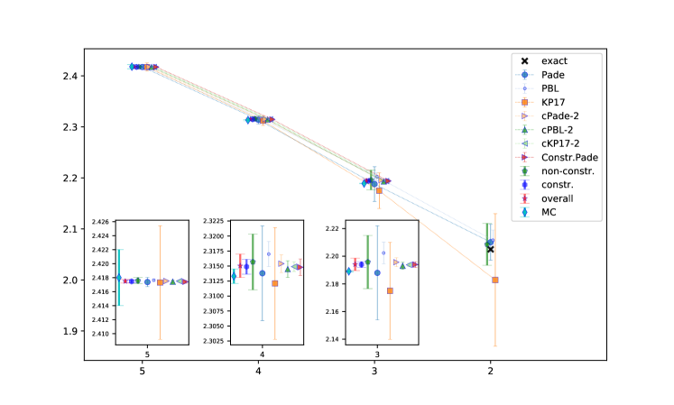
There is a similar picture for which is apparent in Table 17. Again the behaviour of from 2 to 6 dimensions is relatively flat due to the exact values in these dimensions being of a similar order. In this case there are independent data in 4 and 5 dimensions. In the absence of these we could have repeated our final comment for . So it is reassuring that our five loop 4 and 5 dimensional estimates are indeed in excellent agreement with the independent studies. The situation with our 3 dimensional result is in similar accord.
| Reference | |||||
|---|---|---|---|---|---|
| exact | 0.7912 | ||||
| [18] (2015) | 0.4008 | 0.2304 | |||
| MC/srs | [85] (1990) | 0.50(9) | 0.31(5) | 0.27(7) | |
| [89] (1996) | 0.37(4) | ||||
| [88] (1998) | 0.64(2) | ||||
| [90] (1998) | 0.73(8) | ||||
| [93] (1999) | 0.64(5) | ||||
| [104] (2000) | 0.65(2) | ||||
| [91] (2001) | 0.60(8) | 0.5(1) | |||
| [102] (2018) | 0.77(3) | ||||
| [103] (2019) | 0.40(4) | ||||
| overall | 0.66(8) | 0.38(8) | 0.27(7) | ||
| 4 loops | Padé | 0.6(3) | 0.5(2) | 0.37(7) | 0.201(14) |
| PBL | 0.768(4) | 0.583(2) | 0.3956(8) | 0.20593(14) | |
| KP17 | 0.7(2) | 0.51(15) | 0.36(7) | 0.205(15) | |
| cPadé-2 | 0.58(3) | 0.39(2) | 0.205(6) | ||
| cPBL-2 | 0.59425(2) | 0.399952(15) | 0.206613(5) | ||
| cKP17-2 | 0.593(5) | 0.399(5) | 0.206(2) | ||
| Constr. Padé | 0.599(4) | 0.405(5) | 0.209(3) | ||
| non constr. | 0.76(2) | 0.581(13) | 0.395(5) | 0.2059(6) | |
| constr. | 0.5943(5) | 0.4000(4) | 0.20661(10) | ||
| all | 0.76(2) | 0.594(2) | 0.3999(10) | 0.2066(2) | |
| 5 loops | Padé | 0.6(3) | 0.50(15) | 0.36(6) | 0.21(3) |
| PBL | 0.96(5) | 0.68(2) | 0.432(5) | 0.2112(3) | |
| KP17 | 0.7(2) | 0.5(2) | 0.47(9) | 0.215(14) | |
| cPadé-2 | 0.58(3) | 0.39(2) | 0.205(5) | ||
| cPBL-2 | 0.608(6) | 0.411(5) | 0.2095(12) | ||
| cKP17-2 | 0.595(3) | 0.400(3) | 0.2067(12) | ||
| Constr. Padé | 0.597(2) | 0.403(2) | 0.2079(11) | ||
| non constr. | 0.9(2) | 0.65(8) | 0.43(2) | 0.2112(9) | |
| constr. | 0.598(7) | 0.404(6) | 0.208(2) | ||
| all | 0.9(2) | 0.60(2) | 0.409(15) | 0.210(2) |
For the exponent there are again a large number of independent measurements that we have shown in Table 18 though mostly in 3 dimensions. However these and those in 4 dimensions have a wide range of central values as well as a range of errors that are 10% or more in some cases. By contrast to and there is a much larger variation in across the dimensions rising from zero in strictly 6 dimensions as decreases. Despite this both our constrained and unconstrained resummations as well as from four to five loops appear to have a degree of stability. Although our check estimate against the exact two dimensional value is not as good as for other exponents, it is encouraging that our 3 dimensional five loop estimate has overlap with independent data. This is clearly more pronounced for 4 and 5 dimensions. For instance, our final five loop 4 dimensional estimate of for is consistent with the recent 4 dimensional value of , [103].
Finally we arrive at the correction to scaling exponent with the situation summarized in Table 19. As mentioned earlier for our constrained resummations we have taken the exact value in 2 dimensions to be . The independent data is mostly available in 3 dimensions and like covers a wide range from around to . Again similar to , rises from zero to a large 2 dimensional value. The overall picture is that in 3 dimensions our five loop estimates are close to one standard deviation away from our calculated global value from the Monte Carlo data. Though the constrained data in 3 dimensions is in better accord. However the 2 dimensional projected value for our unconstrained resummations is not close to the exact value. What would be useful are independent numerical studies in 4 and 5 dimensions to compare our results with.
| Reference | |||||
|---|---|---|---|---|---|
| exact | 1.5 | ||||
| [18] (2015) | 1.6334 | 1.2198 | 0.7178 | ||
| MC/srs | [85] (1990) | 1.26(23) | 0.94(15) | 0.96(26) | |
| [89] (1996) | 1.13(10) | ||||
| [88] (1998) | 1.61(5) | ||||
| [93] (1999) | 1.62(13) | ||||
| [105] (2010) | 1.0(2) | ||||
| overall | 1.4(3) | 0.94(15) | 1.0(3) | ||
| 4 loops | Padé | 2(2) | 1.5(1.3) | 1.2(5) | 0.73(10) |
| PBL | 2.58(4) | 1.99(2) | 1.388(7) | 0.7544(14) | |
| KP17 | 2.2(8) | 1.8(4) | 1.3(2) | 0.77(3) | |
| cPadé-2 | 1.36(7) | 1.12(6) | 0.70(2) | ||
| cPBL-2 | 1.38(6) | 1.13(6) | 0.70(2) | ||
| cKP17-2 | 1.38(9) | 1.13(9) | 0.70(3) | ||
| Constr. Padé | 1.35(4) | 1.10(5) | 0.70(2) | ||
| non constr. | 2.6(2) | 1.98(9) | 1.38(4) | 0.755(6) | |
| constr. | 1.37(6) | 1.12(6) | 0.70(2) | ||
| all | 2.6(2) | 1.6(3) | 1.30(13) | 0.74(2) | |
| 5 loops | Padé | 2(2) | 1.5(1.1) | 1.2(4) | 0.75(10) |
| PBL | 2.37(5) | 1.88(2) | 1.349(6) | 0.7483(6) | |
| KP17 | 2.8(7) | 2.1(4) | 1.43(12) | 0.76(2) | |
| cPadé-2 | 1.37(8) | 1.13(7) | 0.71(2) | ||
| cPBL-2 | 1.44(9) | 1.19(8) | 0.73(2) | ||
| cKP17-2 | 1.39(9) | 1.14(9) | 0.71(3) | ||
| Constr. Padé | 1.35(5) | 1.10(6) | 0.69(3) | ||
| non constr. | 2.4(2) | 1.89(9) | 1.35(3) | 0.749(3) | |
| constr. | 1.39(11) | 1.15(11) | 0.71(4) | ||
| all | 2.4(2) | 1.7(3) | 1.31(9) | 0.746(11) |
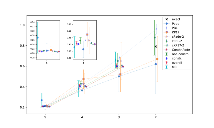
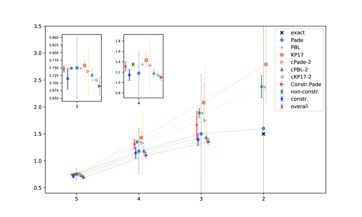
| exponent | |||
|---|---|---|---|
| 0.452(7) | 0.4789(14) | 0.49396(13) | |
| 2.1938(12) | 2.3150(8) | 2.4175(2) | |
| -0.64(4) | -0.75(2) | -0.870(1) | |
| 0.429(4) | 0.658(1) | 0.8452(2) | |
| 1.78(3) | 1.430(6) | 1.1792(7) | |
| 5.16(4) | 3.175(8) | 2.3952(12) | |
| -0.03(1) | -0.084(4) | -0.0547(10) | |
| 0.88(2) | 0.686(2) | 0.5739(1) |
For the most part our focus in this section has been on providing estimates for various exponents. To do this we used the expansion expressions for and and then derived expansions for the other exponents through the scaling and hyperscaling relations of (16). We then applied various different summation methods to each exponent to arrive at estimates for the three dimensions of interest. One question arises as a consequence of this and concerns whether the individual estimates are then consistent with the scaling and hyperscaling relations. Equally another question is which pair of exponents could reasonably be regarded as the ones from which all the other estimates can be accurately described and thereby be our final exponent estimates. To this end we have presented our analysis in Table 20. In particular we have chosen and as our two independent exponents and note that the results using the cKP17-2 technique are the most reasonable to use for final predictions. This is because the two dimensional constraints have been implemented and these two exponents are accurate with a tight error bar in each dimension. Using these cKP17-2 values we have computed the exponents for , , , , and using (16). In the Table the independent values for and are given above the rule with the values derived from scaling relations recorded below. For the remaining two exponents and , their cKP17-2 values have not been included as they are not accessible by scaling or hyperscaling relations and those estimates are already in their respective tables.
Comparing these scaling relation values of Table 20 with those from the direct summation ones given in the earlier tables, none look far out of line. One exception might possibly be the 3 dimensional value of as it appears to be more consistent with the unconstrained analysis. However looking at the extrapolation to 2 dimensions suggests it is probably on a better trajectory. The lack of Monte Carlo or series computations for this exponent means that we have no way of gauging our estimates against an independent analysis. For the other exponents the view is that the individual resummations are consistent with the scaling relations and also with independent data from other methods where that is substantial. In the case of where there are only a few such other cases the estimates in Table 20 are not inconsistent. Our final 3 dimensional estimate for appears to be on the low side but this exponent is difficult to measure accurately. For our 4 and 5 dimensional values are remarkably close to the global average we compiled. While that for 3 dimensions is not as accurate, it does lie within the errors of the global estimate.
In presenting our final estimates in this Table we need to be clear in stating that this shows our results are consistent with scaling relations both by constructing the equations directly and resumming them before comparing the estimates obtained from using two independent summed values in the (hyper)scaling relations. So in essence it is a self-consistency check. By contrast it is usually the case that in the Monte Carlo and series approaches the focus is on one or two specific exponents. Those values are then used to generate the remaining exponents via (16) rather than make extra measurements. So until all techniques have achieved a large degree of computational accuracy it is probably the case that in comparing exponent estimates the overall picture is still not perfect.
7 Conclusions
The main result of this paper is clearly the provision of the five loop renormalization group functions of theory in six dimensions in the scheme. This level of precision could not have been achieved without the use of the graphical function formalism developed in [46, 32]. That method was originally pioneered in four dimensions to renormalize theory to seven loops in the same scheme [32, 57]. To achieve the level of five loop accuracy here required the extension of graphical functions to six dimensions that was provided in [36, 53]. An indication of the advantage of such new and powerful techniques can be gained from the dates that the previous loop order results became available for the cubic theory. The one and two loop renormalization group functions were recorded in the early 70’s [1] with the three loop extension appearing within seven years, [4, 5]. Similar to the extension of theory from five to six loops, there was a quarter of a century lull before theory was renormalized at four loops [18]. The relatively quick extension, in terms of time, to five loops here is suggestive that with suitable investment in the underlying mathematics of the graphical functions approach, higher loop orders are potentially within reach in this and other theories.
Such higher order computations are not purely academic exercises since the second part of our study was to extract improved estimates for critical exponents in two important problems. Both the Lee–Yang edge singularity and percolation problems at criticality lie in separate universality classes but both have a continuum field theory at their heart. The main difference is that the respective versions of the cubic theory are decorated with different symmetry properties. Given that we have renormalized the pure Lagrangian at five loops, it was a relatively simple exercise to include the respective symmetry decorations and determine the two sets of renormalization group functions. From these the expansion of the critical exponents were constructed to before a variety of resummation techniques were applied to extract numerical estimates. Moreover, we devoted a significant part of determining estimates to a careful error analysis using the same formalism provided in [31] for theory. What ought to be recognized is that on the whole not only do the five loop results improve upon the four loop results, as well as showing convergence, but also that there is good agreement with other techniques in both problems for the dimensions of interest. These include Monte Carlo and strong coupling methods to name but a few. In making this remark it should not be overlooked that this includes 3 dimensions where we have summed from down to with a large value of . In one sense this confirms the role of theory as being in the same universality class. What was useful in making this comparison between the exponents from discrete systems and the continuum field theory was collating the available data for the former to produce a global average. The associated error bars were produced with the same routine that we used for the five loop results from the various resummations. In this respect we were endeavouring to compare the picture in the discrete and continuum sides in the same way.
The determination of the five loop renormalization group functions in the core cubic theory opens up the possibility of studying related six dimensional cubic theories to the same level of precision. For instance the conformal bootstrap formalism represents a powerful tool to calculate exponents. It was used in [106] to determine exponents for theory in a variety of representations of the Lie group . While the three loop comparison in that article was in reasonable agreement for various exponents calculated with the bootstrap, the four loop study of [107] gave an improvement towards convergence. It would therefore be interesting, given the accuracy of results in [106], to extend to the study of [107] to five loops. Aside from this particular symmetry of the cubic theory, an intriguing property of with a bi-adjoint symmetry was observed in [108]. For any Lie group it transpires that this theory is asymptotically free due to the two loop coefficient of the function; the one loop term is identically zero. One feature of the four loop result was the appearance of higher order group Casimirs at three loops. This is one order earlier than in four dimensional non-abelian gauge theories. So the bi-adjoint theory offers a window into the type of group Casimirs that could appear in six loop gauge theory functions such as QCD. Although such problems are worth pursuing, the more interesting extension of our current work would clearly be to six loops. This would obviously provide a higher level of precision with which to compare future numerical studies of the discrete spin models in the same universality class. The graphical functions method that was used here, and was successful in extending theory to seven loops [32, 57] should be regarded as a starting point to achieve the six loop renormalization of theory.
Acknowledgements.
We warmly thank A.J. McKane for discussions on the resummation of asymptotic series in quantum field theory. Also JAG thanks R.M. Ziff for encouragement and discussions, and in particular that surrounding the value of in two dimensional percolation theory. We also thank J. Adler for comments and pointing out [80]. The work of MB was supported by the NWO Vidi grant 680-47-551 “Decoding Singularities of Feynman graphs”. The work of JAG was supported by a DFG Mercator Fellowship and in part through the STFC Consolidated grant ST/T000988/1. The work of MVK was supported by Foundation for the Advancement of Theoretical Physics “BASIS” through Grant 18-1-2-43-1. The work of OS was supported by the DFG grant SCHN 1240.
References
- [1] A. Macfarlane and G. Woo, theory in six dimensions and the renormalization group, Nucl. Phys. B 77 (1974) 91.
- [2] E. Ma, Asymptotic freedom and a quark model in six-dimensions, Prog. Theor. Phys. 54 (1975) 1828.
- [3] M.E. Fisher, Yang-Lee edge singularity and field theory, Phys. Rev. Lett. 40 (1978) 1610.
- [4] O.F. de Alcantara Bonfim, J.E. Kirkham and A.J. McKane, Critical exponents to order for models of critical phenomena in dimensions, J. Phys. A 13 (1980) L247.
- [5] O.F. de Alcantara Bonfim, J.E. Kirkham and A.J. McKane, Critical exponents for the percolation problem and the Yang-Lee edge singularity, J. Phys. A 14 (1981) 2391.
- [6] A. Connelly, G. Johnson, S. Mukherjee and V. Skokov, Universality driven analytic structure of QCD crossover: radius of convergence and QCD critical point, Nucl. Phys. A 1005 (2021) 121834 [2004.05095].
- [7] A. Connelly, G. Johnson, F. Rennecke and V. Skokov, Universal location of the Yang-Lee edge singularity in theories, Phys. Rev. Lett. 125 (2020) 191602 [2006.12541].
- [8] R.B. Potts, Some generalized order-disorder transformations, Proc. Cambridge Phil. Soc. 48 (1952) 106.
- [9] K.G. Wilson and M.E. Fisher, Critical exponents in 3.99 dimensions, Phys. Rev. Lett. 28 (1972) 240.
- [10] F. Gliozzi and A. Rago, Critical exponents of the 3d ising and related models from conformal bootstrap, JHEP 10 (2014) 042 [1403.6003].
- [11] X. An, D. Mesterházy and M.A. Stephanov, Functional renormalization group approach to the Yang-Lee edge singularity, JHEP 07 (2016) 041 [1605.06039].
- [12] L. Zambelli and O. Zanusso, Lee-Yang model from the functional renormalization group, Phys. Rev. D 95 (2017) 085001 [1612.08739].
- [13] A. LeClair and J. Squires, Conformal bootstrap for percolation and polymers, J. Stat. Mech. 2018 (2018) 123106 [1802.08911].
- [14] S. Hikami, Conformal bootstrap analysis for the Yang–Lee edge singularity, PTEP 2018 (2018) 053I01 [1707.04813].
- [15] A.L. Pismensky, Calculation of critical index of the -theory in four-loop approximation by the conformal bootstrap technique, Int. J. Mod. Phys. A 30 (2015) 1550138 [1511.03211].
- [16] K.G. Chetyrkin and F.V. Tkachov, Integration by parts: The algorithm to calculate functions in 4 loops, Nucl. Phys. B 192 (1981) 159.
- [17] S. Laporta, High precision calculation of multiloop Feynman integrals by difference equations, Int. J. Mod. Phys. A 15 (2000) 5087 [hep-ph/0102033].
- [18] J.A. Gracey, Four loop renormalization of theory in six dimensions, Phys. Rev. D 92 (2015) 025012 [1506.03357].
- [19] I. Klebanov and A. Polyakov, AdS dual of the critical vector model, Phys. Lett. B 550 (2002) 213 [hep-th/0210114].
- [20] S. Giombi, I.R. Klebanov and B.R. Safdi, Higher spin at one loop, Phys. Rev. D 89 (2014) 084004 [1401.0825].
- [21] L. Fei, S. Giombi and I.R. Klebanov, Critical models in dimensions, Phys. Rev. D 90 (2014) 025018 [1404.1094].
- [22] L. Fei, S. Giombi, I.R. Klebanov and G. Tarnopolsky, Three loop analysis of the critical models in dimensions, Phys. Rev. D 91 (2015) 045011 [1411.1099].
- [23] L. Fei, S. Giombi, I.R. Klebanov and G. Tarnopolsky, Critical models in dimensions and higher spin dS/CFT, JHEP 2015 (2015) [1502.07271].
- [24] J.L. Cardy, Conformal invariance and the Yang-Lee edge singularity in two-dimensions, Phys. Rev. Lett. 54 (1985) 1354.
- [25] D. Friedan, Z. Qiu and S.H. Shenker, Conformal invariance, unitarity and two-dimensional critical exponents, Phys. Rev. Lett. 52 (1984) 1575.
- [26] P. Butera and M. Pernici, Yang-Lee edge singularities from extended activity expansions of the dimer density for bipartite lattices of dimensionality , Phys. Rev. E 86 (2012) 011104 [1206.0872].
- [27] Wikipedia, The Free Encyclopedia, Percolation critical exponents, 2020.
- [28] K.G. Chetyrkin, A.L. Kataev and F.V. Tkachov, Five loop calculations in the model and the critical index , Phys. Lett. B 99 (1981) 147.
- [29] H. Kleinert, J. Neu, V. Schulte-Frohlinde, K.G. Chetyrkin and S.A. Larin, Five loop renormalization group functions of symmetric theory and epsilon expansions of critical exponents up to , Phys. Lett. B 272 (1991) 39 [hep-th/9503230].
- [30] D.V. Batkovich, K.G. Chetyrkin and M.V. Kompaniets, Six loop analytical calculation of the field anomalous dimension and the critical exponent in -symmetric model, Nucl. Phys. B 906 (2016) 147 [1601.01960].
- [31] M.V. Kompaniets and E. Panzer, Minimally subtracted six-loop renormalization of -symmetric theory and critical exponents, Phys. Rev. D 96 (2017) 036016 [1705.06483].
- [32] O. Schnetz, Numbers and functions in quantum field theory, Phys. Rev. D 97 (2018) 085018 [1606.08598].
- [33] O. Schnetz, Hyperlog procedures, https://www.math.fau.de/person/oliver-schnetz/ .
- [34] E. Panzer and O. Schnetz, The Galois coaction on periods, Commun. Num. Theor. Phys. 11 (2017) 657 [1603.04289].
- [35] D.J. Broadhurst and D. Kreimer, Knots and numbers in theory to 7 loops and beyond, Int. J. Mod. Phys. C 6 (1995) 519 [hep-ph/9504352].
- [36] M. Borinsky and O. Schnetz, Graphical functions in even dimensions, 2105.05015.
- [37] A. Vasil’ev, The Field Theoretic Renormalization Group in Critical Behavior Theory and Stochastic Dynamics, Chapman & Hall/CRC, New York (2004), 10.1201/9780203483565.
- [38] R. Zia and D. Wallace, Critical behavior of the continuous component Potts model, J. Phys. A 8 (1975) 1495.
- [39] C. Fortuin and P. Kasteleyn, On the random cluster model. 1. introduction and relation to other models, Physica 57 (1972) 536.
- [40] N.N. Bogoliubow and O.S. Parasiuk, Über die multiplikation der kausalfunktionen in der quantentheorie der felder, Acta Math. 97 (1957) 227.
- [41] N.N. Bogoliubov and D.V. Shirkov, Introduction to the theory of quantized fields, vol. 3 of Interscience monographs in physics and astronomy, Interscience Publishers, New York (1959).
- [42] K.G. Chetyrkin, Combinatorics of -, -, and -operations and asymptotic expansions of Feynman integrals in the limit of large momenta and masses, 1701.08627.
- [43] K.G. Chetyrkin and V.A. Smirnov, -operation corrected, Phys. Lett. B 144 (1984) 419.
- [44] K.G. Chetyrkin and F.V. Tkachov, Infrared -operation and ultraviolet counterterms in the MS-scheme, Phys. Lett. B 114 (1982) 340.
- [45] K.G. Chetyrkin, S.G. Gorishnii, S.A. Larin and F.V. Tkachov, Five loop renormalization group calculations in the in four-dimensions theory, Phys. Lett. B 132 (1983) 351.
- [46] O. Schnetz, Graphical functions and single-valued multiple polylogarithms, Commun. Num. Theor. Phys. 08 (2014) 589 [1302.6445].
- [47] M. Golz, E. Panzer and O. Schnetz, Graphical functions in parametric space, Lett. Math. Phys. 107 (2017) 1177 [1509.07296].
- [48] F. Brown, Single-valued multiple polylogarithms in one variable, Comptes Rendus Math. 338 (2004) 527 .
- [49] F. Brown, Single-valued hyperlogarithms and unipotent differential equations, 2004.
- [50] O. Schnetz, Generalized single-valued hyperlogarithms, (in preparation) (2021) .
- [51] F. Brown, The Massless higher-loop two-point function, Commun. Math. Phys. 287 (2009) 925 [0804.1660].
- [52] E. Panzer, Algorithms for the symbolic integration of hyperlogarithms with applications to Feynman integrals, Comput. Phys. Commun. 188 (2015) 148 [1403.3385].
- [53] M. Borinsky and O. Schnetz, Periods in theory, (in preparation) (2021) .
- [54] R. Beekveldt, M. Borinsky and F. Herzog, The Hopf algebra structure of the -operation, JHEP 20 (2020) 061 [2003.04301].
- [55] M. Borinsky, Tropical Monte Carlo quadrature for Feynman integrals, 2008.12310.
- [56] F. Brown and O. Schnetz, A K3 in , Duke Math. J. 161 (2012) 1817 [1006.4064].
- [57] O. Schnetz, Seven loops , (in preparation) (2021) .
- [58] O. Schnetz, Quantum periods: A census of -transcendentals, Commun. Num. Theor. Phys. 4 (2010) 1 [0801.2856].
- [59] M.V. Kompaniets and A. Pikelner, Critical exponents from five-loop scalar theory renormalization near six-dimensions, 2101.10018.
- [60] L.N. Lipatov, Divergence of the perturbation-theory series and the quasi-classical theory, Sov. Phys. JETP 45 (1977) 216.
- [61] E. Brézin, J.C. Le Guillou and J. Zinn-Justin, Perturbation theory at large order. I. The interaction, Phys. Rev. D 15 (1977) 1544.
- [62] A.J. McKane, Perturbation expansions at large order: results for scalar field theories revisited, J. Phys. A 52 (2019) 055401 [1807.00656].
- [63] A.J. McKane, Vacuum instability in scalar field theories, Nucl. Phys. B 152 (1979) 166.
- [64] J.E. Kirkham and D.J. Wallace, Comments on the field-theoretic formulation of the Yang-Lee edge singularity, J. Phys. A 12 (1979) L47.
- [65] G.A. Kalagov and M.Y. Nalimov, Higher-order asymptotics and critical indexes in the theory, Nucl. Phys. B 884 (2014) 672.
- [66] A. Houghton, J.S. Reeve and D.J. Wallace, High order behavior in field theories and the percolation problem, Phys. Rev. B 17 (1978) 2956.
- [67] A.J. McKane, Asymptotic behaviour of the perturbation expansion in field theories, J. Phys. A 19 (1986) 453.
- [68] S. Caracciolo and D.M. Carlucci, Asymptotic behaviour of the perturbative expansion for 1-state Potts model, http://www.fisica.unisalento.it/~caraccio/ps/mimmo.ps .
- [69] E. Brézin and A.J. McKane, A note on the perturbation expansion in the percolation problem, J. Phys. A 20 (1987) 2235.
- [70] A.J. McKane. Private communication, 2021.
- [71] L.T. Adzhemyan, E.V. Ivanova, M.V. Kompaniets, A. Kudlis and A.I. Sokolov, Six-loop expansion study of three-dimensional -vector model with cubic anisotropy, Nucl. Phys. B 940 (2019) 332 [1901.02754].
- [72] A.A. Vladimirov, D.I. Kazakov and O.V. Tarasov, Calculation of critical exponents by quantum field theory methods, Sov. Phys. JETP 50 (1979) 521.
- [73] D.I. Kazakov, O.V. Tarasov and D.V. Shirkov, Analytic continuation of the results of perturbation theory for the model to the region , Theor. Math. Phys. 38 (1979) 9.
- [74] J.C. Le Guillou and J. Zinn-Justin, Accurate critical exponents from the -expansion, J. Physique Lett. 46 (1985) 137.
- [75] R. Guida and J. Zinn-Justin, Critical exponents of the -vector model, J. Phys. A 31 (1998) 8103 [cond-mat/9803240].
- [76] S. Lai and M. Fisher, The universal repulsive-core singularity and Yang–Lee edge criticality, J. Chem. Phys. 103 (1995) 8144.
- [77] N. Araúji, P. Grassberger, B. Kahng, K. Schrenk and R. Ziff, Recent advances and open challenges in percolation, Eur. J. Phys. Spec. Top. 822 (2014) 2307 [1404.5325].
- [78] D. Stauffer, Scaling theory of percolation clusters, Phys. Rept. 54 (1979) 1.
- [79] G. Parisi and N. Sourlas, Critical Behavior of Branched Polymers and the Lee-Yang Edge Singularity, Phys. Rev. Lett. 46 (1981) 871.
- [80] J. Adler, Y. Meir, A. Harris, A. Aharony and J. Duarté, Series study of random animals in general dimensions, Phys. Rev. B 38 (1988) 4941.
- [81] D. Stauffer and A. Aharony, Introduction to percolation theory, Taylor & Francis (1992), 10.1201/9781315274386.
- [82] P.J. Reynolds, H.E. Stanley and W. Klein, Large-cell Monte Carlo renormalization group for percolation, Phys. Rev. B 21 (1980) 1223.
- [83] B. Nienhuis, -cluster correlations in four- and five-dimensional percolation, J. Phys. A 15 (1982) 199.
- [84] R. Ziff, Correction-to-scaling exponent for two-dimensional percolation, Phys. Rev. E 83 (2011) 020107(R) [1101.0807].
- [85] J. Adler, Y. Meir, A. Aharony and A. Harris, Series study of percolation moments in general dimension, Phys. Rev. B 41 (1990) 9183.
- [86] A. Sur, J. Lebowitz, J. Marro, M. Kalos and S. Kirkpatrick, Monte Carlo studies of percolation phenomena for a simple cubic lattice, J. Stat. Phys. 15 (1976) 345.
- [87] H. Nakanishi and H. Stanley, Scaling studies of percolation phenomena in systems of dimensionality two to seven: cluster numbers, Phys. Rev. B 22 (1980) 2466.
- [88] C. Lorenz and R. Ziff, Precise determination of the bond percolation thresholds and finite-size scaling corrections for the sc, fcc, and bcc lattices, Phys. Rev. E 57 (1998) 230 [cond-mat/9710044].
- [89] H. Ballesteros, L. Fernandez, V. Martin-Mayor, A.M. Sudupe, G. Parisi and J. Ruiz-Lorenzo, Measures of critical exponents in the four-dimensional site percolation, Phys. Lett. B 400 (1997) 346 [hep-lat/9612024].
- [90] N. Jan and D. Stauffer, Random site percolation in three dimensions, Int. J. Mod. Phys. C 9 (1998) 341.
- [91] D. Tiggemann, Simulation of percolation on massively parallel computers, Int. J. Mod. Phys. C 12 (2001) 871 [cond-mat/0106354].
- [92] M. Levenshteĭn, B. Shklovskiĭ, M. Shur and A. Éfros, The relation between the critical exponents of percolation theory, Zh. Eksp. Teor. Fiz. 69 (1975) 386.
- [93] H. Ballesteros, L. Fernandez, V. Martin-Mayor, A.M. Sudupe, G. Parisi and J. Ruiz-Lorenzo, Effect of dilution on first order transitions: the three-dimensional three states Potts model, Phys. Rev. B 61 (2000) 3215 [cond-mat/9906195].
- [94] J. Wang, Z. Zhou, W. Zhang, T. Garoni and Y. Deng, Bond and site percolation in three dimensions, Phys. Rev. E 87 (2013) 052107 [1302.0421].
- [95] H. Hu, H. Blöte, R. Ziff and Y. Deng, Short-range correlations in percolation at criticality, Phys. Rev. E 90 (2014) 042106 [1406.0130].
- [96] X. Xu, J. Junfeng, J.-P. Lv and Y. Deng, Simultaneous analysis of three-dimensional percolation models, Front. Phys. 9 (2014) 113 [1310.5399].
- [97] Z. Koza and J. Pola, From discrete to continuous percolation in dimensions 3 to 7, J. Stat. Mech. 2016 (2016) 103206 [1606.08050].
- [98] X. Tan, Y. Deng and J.L. Jacobsen, -cluster correlations in four- and five-dimensional percolation, Front. Phys. 15 (2020) 41501 [2006.10981].
- [99] M. Sykes, D. Gaunt and J. Essam, The percolation probability for the site problem on the face- centred cubic lattice, J. Phys. A 9 (1976) L43.
- [100] G. Paul, R. Ziff and H. Stanley, Percolation threshold, Fisher exponent, and shortest path exponent for four and five dimensions, Phys. Rev. B 64 (2001) 026115 [cond-mat/0101136].
- [101] D. Tiggemann, Percolation on growing lattices, Int. J. Mod. Phys. C 17 (2006) 1141 [cond-mat/0604418].
- [102] S. Mertens and C. Moore, Percolation thresholds and fisher exponents in hypercubic lattices, Phys. Rev. E 98 (2018) 022120 [1806.08067].
- [103] Z. Xun and R. Ziff, Precise bond percolation thresholds on several four-dimensional lattices, Phys. Rev. Research 2 (2020) 013067 [1910.11408].
- [104] J.-C. Gimel, T. Nicolai and D. Durand, Size distribution of percolating clusters on cubic lattices, J. Phys. A 33 (2000) 7687.
- [105] B. Kozlov and M. Laguës, Universality of 3d percolation exponents and first-order corrections to scaling for conductivity exponents, Physica A 389 (2010) 5339.
- [106] Y. Pang, J. Rong and N. Su, theory with flavor symmetry in dimensions: 3-loop renormalization and conformal bootstrap, JHEP 12 (2016) 057 [1609.03007].
- [107] J.A. Gracey, symmetric theory at four loops, Phys. Rev. D 95 (2017) 065030 [1703.03782].
- [108] J.A. Gracey, Asymptotic freedom from the two-loop term of the function in a cubic theory, Phys. Rev. D 101 (2020) 125022 [2004.14208].