SPatchGAN: A Statistical Feature Based Discriminator for Unsupervised Image-to-Image Translation

Abstract

For unsupervised image-to-image translation, we propose a discriminator architecture which focuses on the statistical features instead of individual patches. The network is stabilized by distribution matching of key statistical features at multiple scales. Unlike the existing methods which impose more and more constraints on the generator, our method facilitates the shape deformation and enhances the fine details with a greatly simplified framework. We show that the proposed method outperforms the existing state-of-the-art models in various challenging applications including selfie-to-anime, male-to-female and glasses removal.

1 Introduction

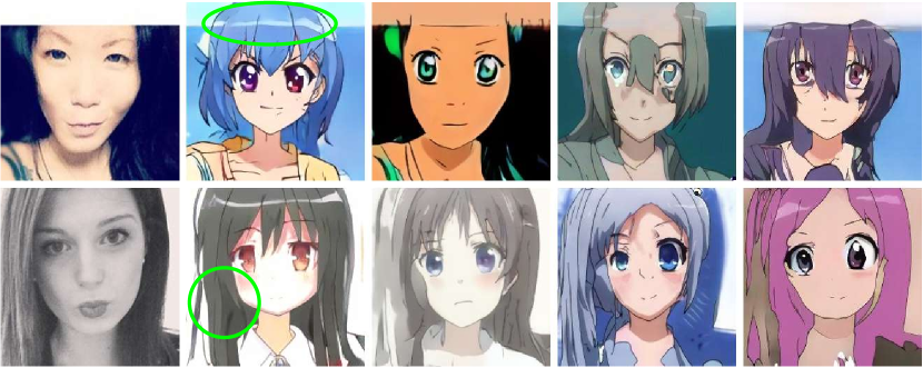
    Input        SPatchGAN     U-GAT-IT     Council-GAN   ACL-GAN

(a) Selfie-to-anime

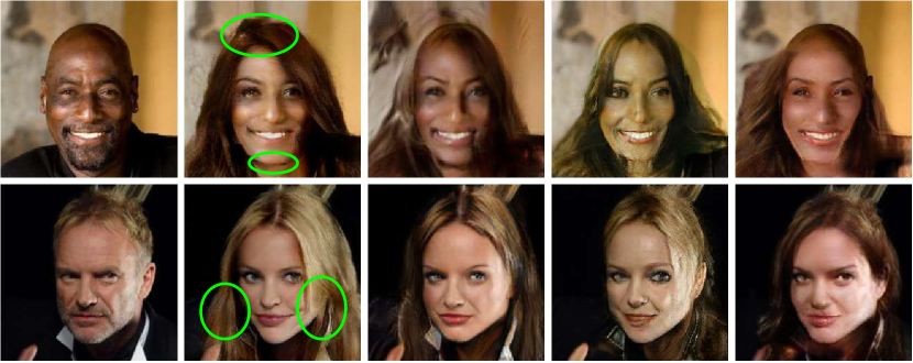
    Input        SPatchGAN     U-GAT-IT     Council-GAN   ACL-GAN

(b) Male-to-female

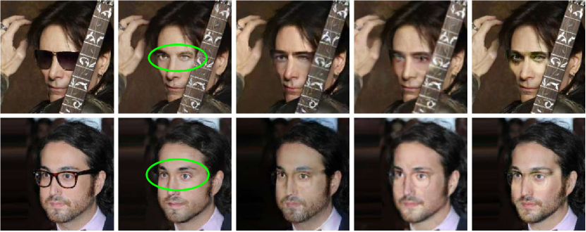
    Input        SPatchGAN     U-GAT-IT     Council-GAN   ACL-GAN

(c) Glasses removal

Figure 1: Example results for our SPatchGAN and the baselines. Our method generates natural looking hairstyle in Figure 1(a) and Figure 1(b), and suppresses the traces of glasses in Figure 1(c). The improvements in shape deformation are highlighted with green circles.

Unsupervised image-to-image translation has become an area of growing interest in computer vision. Powered by generative adversarial networks (GANs) [7], recent works [37, 17, 20, 31, 1, 10, 6, 30, 19] are able to change the local texture and style of the images without the assistance of any paired data. However, these methods still have difficulty with tasks which require a larger shape deformation. Our goal is to improve unsupervised image-to-image translation for applications which involve geometric changes between the source and the target domains.

GANs are trained by a game between a generator network and a discriminator network. At the core of the modern unsupervised image translation frameworks [37, 10, 16, 27, 26, 35] is a PatchGAN discriminator [11]. Instead of giving a single real vs. fake probability for the whole image, PatchGAN produces multiple outputs for multiple overlapping image patches. It helps with the convergence of the network by involving less parameters and stopping at a relatively low-level scale [11].

PatchGAN is feasible for identifying a specific type of texture all over the image, since it processes all the patches by the same set of convolutional weights. However, we find it less capable of dealing with complicated shape changes like selfie-to-anime. In such a case, the discriminative features for one area, e.g., the eyes of an anime face, can be very different from another area, e.g., the hair. Therefore, it becomes difficult to make an accurate and stable decision for every patch.

A related problem is that PatchGAN alone cannot guarantee the stability of an unsupervised image translation network. Various constraints have been proposed to stabilize and improve the training process, including the cycle constraints [37, 17] and the shared latent space assumptions [20, 10]. The constraints are applied on the generator to help alleviate some typical problems such as mode collapse. However, these methods often create a conflict between the interest of GANs and the additional constraints, resulting in incompletely translation. E.g., it is challenging to reshape the hair properly in Figure 1(a) and Figure 1(b), and remove the traces of glasses in Figure 1(c).

The above issues can be potentially solved if one can stabilize the discriminator itself instead of introducing more constraints on the generator. With this motivation, we propose SPatchGAN, an improved multi-scale discriminator architecture which leverages the statistical features over patches. The network benefits from the stability and global view of statistical features at the low-level scales, and the strong discrimination capability at the high-level scales. All the scale levels are jointly optimized in a unified network. With the improved discriminator, we are able to reduce the full cycle constraints to a weak form that only operates on the forward cycle and the low resolution images.

The experiments demonstrate that our method is superior to the existing state-of-the-art methods. The main contributions are:

• Our novel discriminator architecture stabilizes the network by matching the distributions of the statistical features, and employing a shared backbone for the multiple scales.

• We propose a simplified framework that reduces the conflicts between GANs and the other constraints, and facilitates the shape deformation.

2 Related Work

GANs. GANs have provided a powerful tool for matching two distributions, and delivered promising results for various applications. However, GANs are usually non-ideal in practice due to some stability issues such as mode collapse and oscillation [23].

Various methods [29, 23, 2, 8, 22, 25] have been studied to stabilize GANs. Our work is inspired by the feature matching technique [29] which aligns the features of the generated images with the real images at an intermediate layer. We enhance the feature matching technique by considering distribution matching instead of minimizing the L1 or L2 distance. Moreover, our method operates on the statistics of activations instead of individual activation values. We also extend the method to multiple scales.

Many studies [24, 28, 13, 34, 5, 14, 12, 15] are related to improving GANs for random image generation, but these methods are not always applicable to image translation. E.g., MSG-GAN [12] facilitates the flow of gradients by connecting the matching layers of the generator and discriminator, but there is no such layer correspondence in the typical image translation networks. Therefore, it is necessary to specifically optimize the network architecture for image translation.

Discriminator Structures for Image Translation. The discriminator in the original GAN framework [7] is simply a binary classifier. For supervised image translation, Isola et al. [11] propose the PatchGAN discriminator to classify if each image patch is real or fake. The responses of all the patches are averaged to provide the final output. PatchGAN is initially designed for improving the high-frequency part of the generated image, while the correctness of the overall structure is guaranteed by the supervision signal.

The PatchGAN structure has been extended to multiple scales [33] to cover the low frequency part as well, and has been widely adopted by the latest unsupervised image translation networks [10, 16, 26, 35]. Among these methods, U-GAT-IT [16] applies PatchGAN on two scales and uses a Class Activation Map (CAM) [36] based attention module. MUNIT [10] and ACL-GAN [35] collect the outputs from three scales. The multi-scale PatchGAN usually has an independent network for each scale, e.g., the discriminator in [10, 35] consists of three networks respectively for the raw image, the $1/4$ sized image and the $1/16$ sized image. Different from the above methods, we switch our attention from the individual patches to the statistical features over patches, and employ a unified network for multiple scales.

Unsupervised Image Translation Frameworks. A cycle based framework [37, 17] is widely used to stabilize GANs for unsupervised image translation. In this framework, two generators are jointly optimized to enforce a forward cycle constraint and a backward cycle constraint. Though the framework is effective in preventing mode collapse, it often causes irrelevant traces of the source image to be left on the generated image [26, 35]. The cycle constraints are often used together with an identity mapping constraint [31] which reconstructs a target domain image with the generator. CUT [27] achieves a similar goal with cycle constraints through a different approach, enforcing the corresponding elements of the source and generated images to be mapped to a similar feature vector. In our work, the cycle constraints are relaxed to reduce the side effects.

Some recent works [10, 1, 19] further consider the problem of generating multiple output images for a given source image. MUNIT [10] supports multimodality by encoding the source image into a content code and a style code. Council-GAN [26] further considers distribution matching among multiple generators, while ACL-GAN [35] considers distribution matching between the cycle output and the identity mapping output. The multimodal frameworks are usually more complicated than the unimodal frameworks, e.g., MUNIT requires the reconstruction of the image from the content and style codes, and the reconstruction of the codes from the image. In this paper we mainly focus on the unimodal case for simplicity, but we also compare our results to the the state-of-the-art multimodal methods. The applicability of our method in multimodal translation is studied in the supplementary materials.

3 Model

Our model consists of a forward generator $G$, an SPatchGAN discriminator $D$, and a backward generator $B$ that operates on the low resolution images. The forward generator translates a source image $x_{1}$ to a generated image $G(x_{1})$. $G$ and $D$ play an adversarial game, in which $D$ aims to distinguish the generated images from the real images, while $G$ aims to fool the discriminator. $B$ is jointly optimized with $G$ to ensure the similarity between the source image and the generated image, and to stabilize the network.

The source domain and the target domain for the image translation task are denoted $\mathcal{X}_{1}$ and $\mathcal{X}_{2}$. We denote the distribution of source images $x_{1}\in\mathcal{X}_{1}$ as $p^{src}(x)$, the distribution of real images $x_{2}\in\mathcal{X}_{2}$ as $p^{data}(x)$, and the distribution of the generated images $G(x_{1})$ as $p^{g}(x)$. The goal is to match $p^{g}(x)$ with $p^{data}(x)$, and preserve the common characteristics between the two domains during the translation.

3.1 Discriminator Structure

Our discriminator structure is shown in Figure 2. $D$ takes an image $x$ as the input, which can be either a real image $x_{2}$ or a generated image $G(x_{1})$. $D$ produces multiple outputs $D_{m,n}(x)$, $m=1,2,...M$, $n=1,2,...N$, where $M$ is the number of scales, $N$ is the number of statistical features. $D$ has an initial feature extraction block, followed by $M$ scales. Each scale consists of a downsampling block, an adaptation block, a statistical feature calculation block and $N$ multilayer perceptrons (MLPs). We show only two scales in Figure 2 for simplicity, starting from the scale at the lowest level, i.e., scale 1.

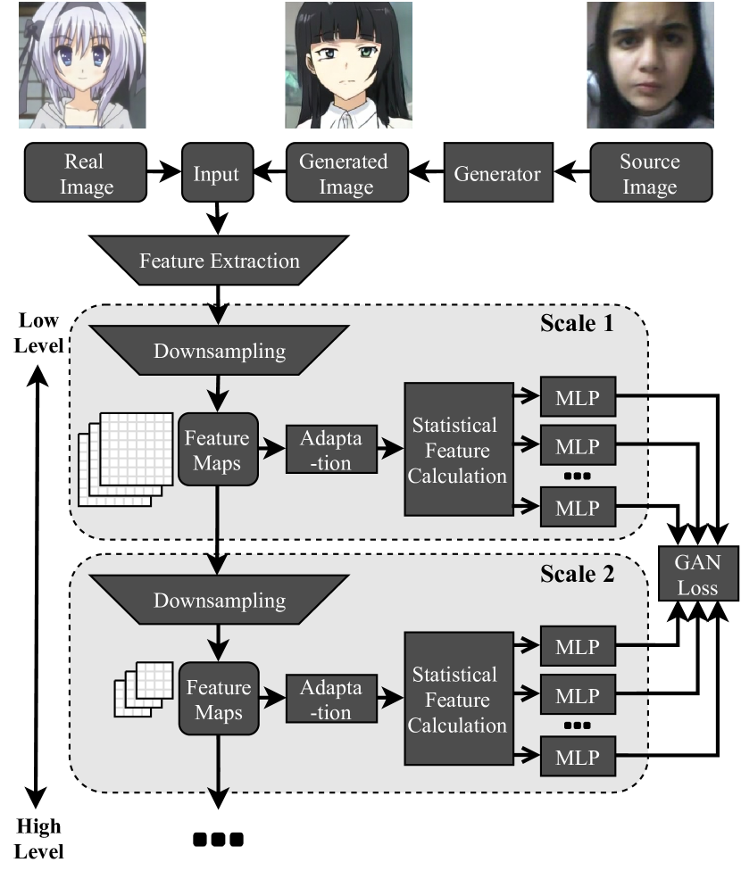
Figure 2: Our multi-scale discriminator structure. The feature maps of each scale are processed by an adaptation block, a statistical feature calculation block and $N$ MLPs to generate $N$ outputs.

The feature maps of each scale are generated by the corresponding downsampling block, and are reused by the higher level scales. They are processed by an adaptation block to adjust the features specifically for the current scale. The adapted feature maps at the $m$-th scale are denoted as $h_{m}(x)\in\mathbb{R}^{H_{m}\times W_{m}\times C_{m}}$, where $H_{m}$, $W_{m}$ and $C_{m}$ are the height, width and number of channels of the adapted feature maps. $h_{m}$ is the function for the backbone network of the $m$-th scale. It is jointly defined by the initial feature extraction block, the downsampling blocks up to the $m$-th scale and the adaptation block at the $m$-th scale. Each element of the adapted feature maps corresponds to a patch of the input image. A higher level has a larger patch size.

The adapted feature maps are sent to the statistical feature calculation block to generate the channel-wise statistics. For the $m$-th scale, $N$ statistical feature vectors $s_{m,n}(x)\in\mathbb{R}^{C_{m}}$, $n=1,2,...N$ are calculated,

$$s_{m,n}(x)=g_{n}(h_{m}(x)).$$ (1)

$g_{n}$ is the function that calculates the $n$-th statistical feature.

Each statistical feature vector is further processed by a multilayer perceptron (MLP) to finally generate a scalar output,

$$D_{m,n}(x)=f_{m,n}(s_{m,n}(x)),$$ (2)

where $f_{m,n}$ is defined by the MLP for the $n$-th statistical feature at the $m$-th scale.

Different from the individual patch based methods, the output of our discriminator is derived from the statistical features $s_{m,n}(x)$. The statistical features are usually more stable than the individual patches, since each of their elements is calculated over $H_{m}W_{m}$ patches. In contrast to the limited perceptive field of individual patches, every statistical feature is about the whole image. The global view is helpful for verifying the correctness of shape deformation, e.g., the change of the hairstyle. Furthermore, we employ a dedicated MLP for each statistical feature, rather than the shared convolutional weights in PatchGAN. This makes each output of our discriminator more accurate.

3.2 Analysis of Statistical Feature Matching

Our discriminator is designed to match the statistical features of the generated images with the real images. At a high-level scale, matching the statistical features is similar to fully matching the input distributions, since the high-level features are very discriminative. It also implies the difficulty for achieving a perfect matching at the high level. However, we can expect to match the statistical features at the lower levels with more confidence.

An important assumption in the original GAN framework is training $D$ until optimal after each update of $G$ [7]. For a given input $x$, the optimal output is

$$D^{*}(x)=\frac{p^{data}(x)}{p^{data}(x)+p^{g}(x)}.$$ (3)

However, this assumption is usually not met in practice, where $D$ is typically a complicated neural network to deal with a high dimensional input $x$. It is very challenging to train $D$ until optimal due to issues such as the saddle points and the local minimum.

Instead of directly matching the distributions of the input images, our target is matching the distributions of the statistical features $s_{m,n}(x)$ in Eq. 1. We consider $s_{m,n}(x)$ as a feature input, and its corresponding MLP $f_{m,n}$ as a feature discriminator. $s_{m,n}(x)$ as an input has a much lower dimension than the original input $x$, so a simple MLP can serve as its discriminator with enough capacity. This makes it easier to train the feature discriminator $f_{m,n}$ to optimal. Similar to Eq. 3, the optimal output of the feature discriminator is

$$D_{m,n}(x) =f^{*}_{m,n}(s_{m,n}(x))$$ (4)

$$=\frac{p^{data}_{m,n}(s_{m,n}(x))}{p^{data}_{m,n}(s_{m,n}(x))+p^{g}_{m,n}(s_{m,n}(x))},$$

where $p^{data}_{m,n}(s)$ and $p^{g}_{m,n}(s)$ are the distributions of $s_{m,n}(x)$ for the real and generated images respectively. We expect $D_{m,n}(x)$ to be close to $0.5$ when the two distributions are well matched.

On the other hand, there is an disadvantage of the feature input $s_{m,n}(x)$. Unlike the original input image, the feature input additionally depends on a part of the discriminator $h_{m}$ according to Eq. 1. As a result, the feature discriminator is simultaneously updated with its input distributions $p^{data}_{m,n}(s)$ and $p^{g}_{m,n}(s)$, even if the generator is fixed. The main challenge for the feature discriminator turns out to be that its knowledge about the feature inputs is not fully up to date. Put simply, the feature discriminator is non-ideal unless $h_{m}$ is fixed.

As the backbone of the discriminator, $h_{m}$ is optimized to make the statistical features discriminative. We cannot fix $h_{m}$, but we can stabilize $h_{m}$ as much as possible. This is where our network structure plays an important role. The layers in $h_{m}$ are shared by multiple scales and multiple outputs, so they are unlikely to be changed drastically according to one output. $h_{m}$ at a low-level scale is especially stable, since it contains less layers, and receives optimization signals from more higher level outputs. Moreover, the statistical features are further stabilized by the calculation over multiple patches, especially at a low-level scale where the number of patches is large.

As long as the feature inputs are slow varying compared to the feature discriminator, the output of the discriminator becomes relatively accurate. As a result, $G$ can be optimized in the correct direction to match $p^{g}_{m,n}(s)$ with $p^{data}_{m,n}(s)$ according to the signals from $D$. Though the distributions are dependent on the non-cooperative $h_{m}$, chances are they can be matched by $G$ when $h_{m}$ is stable enough.

Therefore, a good match between low-level statistical features can be practically achieved using the discriminator designed in our fashion, encouraging the generator to avoid the potential flaws that would break the distribution matching. Our experiments demonstrate that such statistical feature matching mechanism effectively alleviates mode collapse and stabilizes the training process.

3.3 Training Framework

Our training framework has three objectives. An adversarial loss is employed for matching the distributions of the statistical features. A weak cycle loss and an identity loss are added to keep the generated image correlated with the input image, and to further stabilize the network.

Adversarial Loss. We adopt the Least Squares GANs (LSGANs) objective [22] instead of the original GAN objective [7] for stable training. We use the binary 0-1 coding variant to keep the optimal output of the discriminator unchanged. The loss function for $D$ is averaged over multiple scales and multiple statistical features,

$$\begin{split}L^{adv}_{D}=\frac{1}{MN}\sum_{m}\sum_{n}(\mathbb{E}_{x\sim p^{data}(x)}[(D_{m,n}(x)-1)^{2}]\\ +\mathbb{E}_{x\sim p^{src}(x)}[D_{m,n}(G(x))^{2}]).\end{split}$$ (5)

Similarly, the adversarial loss function for $G$ is

$$\begin{split}L^{adv}_{G}=\frac{1}{MN}\sum_{m}\sum_{n}(\mathbb{E}_{x\sim p^{src}(x)}[(D_{m,n}(G(x))-1)^{2}]).\end{split}$$ (6)

Weak Cycle Loss. In the original cycle based framework, a forward cycle constraint $x_{1}=B(G(x_{1}))$ and a backward cycle constraint $x_{2}=G(B(x_{2}))$ are necessary for preventing mode collapse [37]. After improving the discriminator, we find the network stable enough with the forward cycle only. We simply remove the backward cycle, and thus reduce the complexity by half.

Moreover, we further simplify the backward generator $B$, i.e., the generator from the target domain to the source domain. Compared to the original backward generator which operates on the full sized images, ours reconstructs a low resolution source image from a low resolution generated image. The weak cycle loss function is

$$L^{cyc}=\mathbb{E}_{x\sim p^{src}(x)}[\lVert u(x)-B(u(G(x)))\rVert_{1}],$$ (7)

where $u(x)$ is the operation to resize a full sized image to a low resolution image.

Since the weak cycle constraint is applied on the low resolution images, only the low frequency information of the source image is required to be preserved in the generated image. Compared to the full cycle constraints, the weak cycle constraint suppresses the leftovers from the source image, and facilitates the shape deformation. On the other hand, it still helps to keep the overall structure of the source image, such as the pose of face in the selfie-to-anime case. We know that some high frequency information may also need to be preserved depending on the application, and leave this job to the identity loss.

Identity Loss. Our identity loss is similar to that in [37, 16], with the exception that the loss is applied to the target domain only. Unlike the weak cycle loss, the identity loss is applied on the full sized images. The identity loss function is

$$L^{id}=\mathbb{E}_{x\sim p^{data}(x)}[\lVert x-G(x)\rVert_{1}].$$ (8)

The identity loss turns the generator into an autoencoder for the target domain. This helps to preserve the common parts in the source and the target domains, such as the background in the glasses removal case. Compared to the cycle loss, the identity loss is less likely to conflict with the adversarial loss, since the input for the generator is taken from a different domain.

Full Objective. The total loss of the forward and backward generators is the weighted sum of Eq. 6, Eq. 7 and Eq. 8,

$$L_{G}=\lambda^{adv}L^{adv}_{G}+\lambda^{cyc}L^{cyc}+\lambda^{id}L^{id},$$ (9)

The objective of the generators is minimizing $L_{G}$. The objective of the discriminator is minimizing its loss in Eq. 5.

3.4 Implementation

We describe the basic structure and parameter settings of our model in this section. The details are available in the supplementary materials. The height and width of the input images are assumed to be $H_{0}$ and $W_{0}$.

Discriminator. We set the number of scales to be $M=4$. The height and width of the feature maps are downsampled to $\frac{H_{0}}{4}$ and $\frac{W_{0}}{4}$ by the feature extraction block, and further downsampled by a factor of 2 in each scale. The convolutional layers for downsampling are similar to those in the multi-scale PatchGAN [10, 26, 35]. The adaptation block consists of two $1\times 1$ convolutional layers. We use spectral normalization [25] in the discriminator.

Our discriminator is flexible enough to incorporate with various kinds of statistical features. In our experiments, we find that a good performance can be achieved with three basic ones, i.e., $N=3$. The function $g_{1}$ in Eq. 1 calculates the channel-wise mean values using global average pooling. $g_{2}$ calculates the channel-wise maximum values using global max pooling. $g_{3}$ calculates the channel-wise uncorrected standard deviation for each feature map. In our implementation, the statistical feature calculation layers are pre-defined rather than learnable, i.e., the contributions of all patches are taken into account in a fixed manner. In contrast, a learnable channel-wise reduction layer may dynamically switch its attention on different patches during the training process, making the calculated features less robust.

Generator. The generator in our framework can be chosen independently of the discriminator. In our implementation, we adopt a modified version of CycleGAN [37] as our forward and backward generator. To further facilitate shape deformation, we apply the residual blocks to feature maps of size $\frac{H_{0}}{8}\times\frac{W_{0}}{8}$ instead of $\frac{H_{0}}{4}\times\frac{W_{0}}{4}$. Accordingly, the input dimensions of the backward generator are resized to $\frac{H_{0}}{8}\times\frac{W_{0}}{8}$. We also use layer normalization [3] instead of instance normalization [32] in the upsampling layers to alleviate the blob artifact problem [15].

4 Experiments

4.1 Experiment Setup

Datasets. Similar to [26, 35], we evaluate SPatchGAN on three tasks including selfie-to-anime, male-to-female and glasses removal.

Selfie-to-Anime. The selfie-to-anime dataset [16] contains 3,400 / 100 selfie images and 3,400 / 100 anime face images in the training / test set. The image size is $256\times 256$.

Male-to-Female. The male-to-female dataset [26] contains face images cropped from CelebA [21]. The training / test set contains 68,261 / 16,173 images of male, and 94,509 / 23,656 images of female. The image size is $218\times 178$.

Glasses Removal. The original glasses removal dataset [26] contains face images cropped from CelebA [21] for both male and female. It has a data imbalance problem that there are much more images of male with glasses than female with glasses. As a side effect, the face may become more feminine after removing the glasses [26, 35]. To avoid this problem and focus on the glasses removal task, we only use the male images in our experiments. The training / test set contains 8,366 / 2,112 images of male with glasses, and 59,895 / 14,061 images of male without glasses. The image size is the same as male-to-female.

Baseline Models. We compare our SPatchGAN to the state-of-the-art models for unsupervised image translation, including CycleGAN [37], MUNIT [10], U-GAT-IT [16], CUT [27], Council-GAN [26] and ACL-GAN [35]. CycleGAN and CUT uses a single scale PatchGAN discriminator, while the others use the multi-scale PatchGAN. CycleGAN and U-GAT-IT are based on the cycle constraints. CUT is based on a contrastive learning approach which maximizes the mutual information between the source and generated images. MUNIT, Council-GAN and ACL-GAN are based on a partially shared latent space assumption. We use the official pre-trained models if available, including the selfie-to-anime and male-to-female models of Council-GAN, and the selfie-to-anime model of U-GAT-IT. The other results are reproduced using the official code base.

Evaluation Metrics. We adopt two metrics, the Fréchet Inception Distance (FID) [9] and the kernel inception distance (KID) [4], for the quantitative evaluation. FID is a widely used metric for comparing the distributions of the real and generated images. KID is an improved metric which takes additional aspects of the distributions into account, and is unbiased.

Training. Our model is trained with $\lambda^{adv}=4$ and $\lambda^{id}=10$ for all the datasets. $\lambda^{cyc}$ is set to $20$, $10$ and $30$ respectively for selfie-to-anime, male-to-female and glasses removal.

We use an Adam [18] optimizer with $\beta_{1}=0.5$ and $\beta_{2}=0.999$. We also use a weight decay at rate of 0.0001. The models are trained for 500k iterations with a batch size of four. The learning rate is 0.0001 for the first 100k iterations and linearly decayed to 0.00001. The training takes about 2 hours per 10k iterations on a NVIDIA Tesla V100 GPU. As a reference, U-GAT-IT [16] in its light mode costs about 3.5 hours per 10k iterations with the same batch size and infrastructure. The speed-up of our method is from the simplified training framework.

4.2 Ablation Studies

We compare SPatchGAN to several variants, including 1) removing the channel-wise mean feature, 2) removing the channel-wise maximum feature. 3) removing the channel-wise standard deviation feature, 4) replacing the whole SPatchGAN discriminator with the multi-scale PatchGAN discriminator in [10, 35].

The generated images are shown in Figure 3. We observe some minor defects when one of the statistical features is removed, e.g., inconsistent color of the two eyes, redundant lines on the face, and blurred local texture. The multi-scale PatchGAN often generates collapsed eyes, indicating that it failed to ensure the correctness of the individual patches when the constraints on the generator are relaxed.

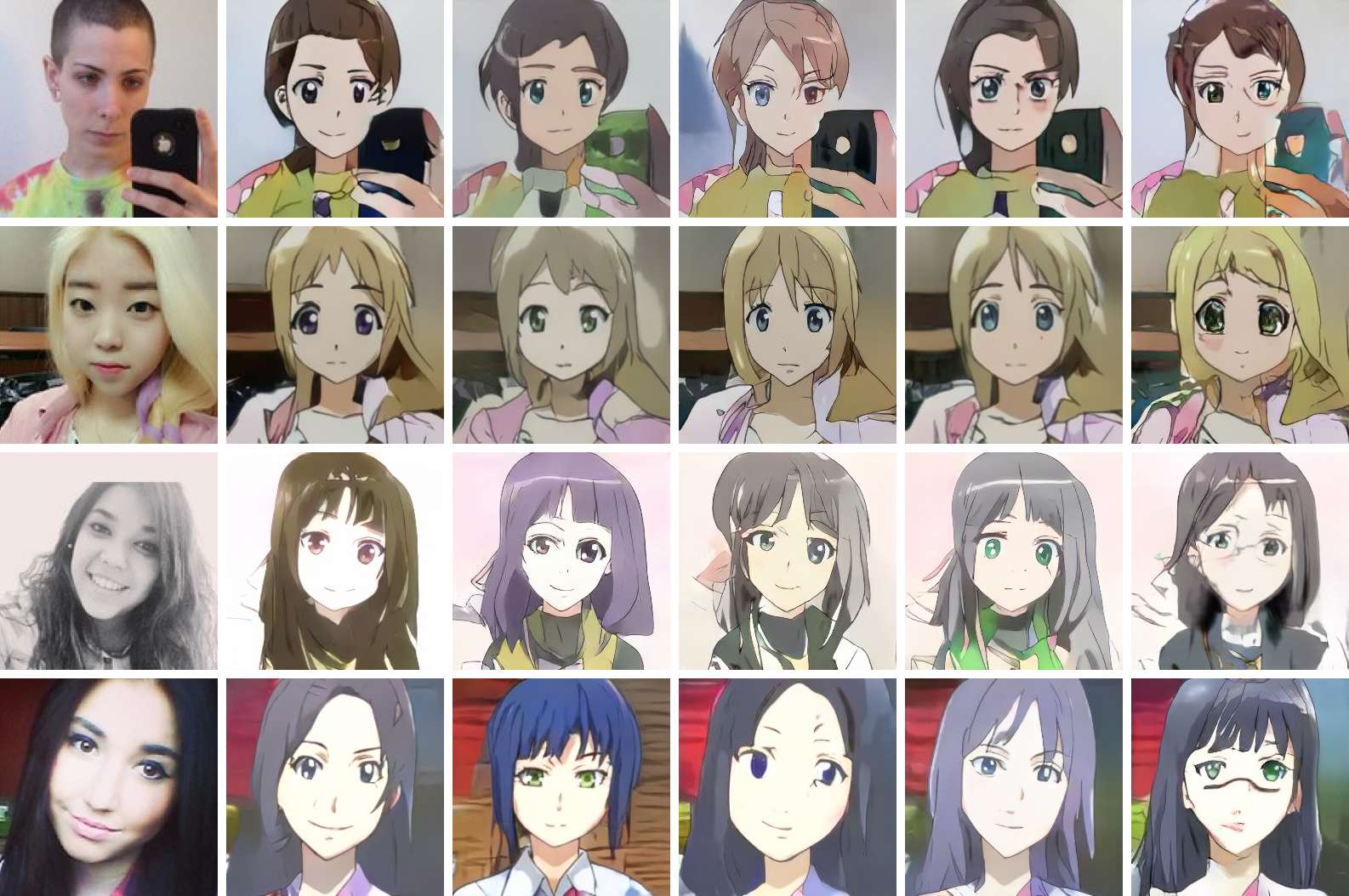
    Input     SPatchGAN   w/o Mean   w/o Max   w/o Stddev   PatchGAN

Figure 3: Generated images of the ablation study cases for selfie-to-anime.

The quantitative results are summarized in Table 1. As a reference, we also include the average FID and KID of the real images to demonstrate the performance in the ideal case. For the real image case, the training images of the target domain are compared to the testing images of the target domain. For the other cases, the generated images are compared to the testing images of the target domain. SPatchGAN has the best FID and KID scores, since it considers the full set of statistical features that reflect the key aspects of the distribution. However, there is still a gap between SPatchGAN and the real images, implying the difficulty of full distribution matching. The performance slightly deteriorate when one of the statistical features is removed. The multi-scale PatchGAN performs much worse than the SPatchGAN based methods in terms of both FID and KID.

Model	FID	KID
SPatchGAN	83.3	0.0214
SPatchGAN w/o Mean	84.1	0.0228
SPatchGAN w/o Max	83.8	0.0223
SPatchGAN w/o Stddev	84.9	0.0214
Multi-scale PatchGAN	94.0	0.0362
Real images	76.7	0.0030

Table 1: Quantitative results of the ablation study cases for selfie-to-anime. Lower is better.

Figure 4: The discriminator outputs of SPatchGAN for the generated images in the selfie-to-anime case.

Model	Selfie-to-Anime		Male-to-Female		Glasses Removal
	FID	KID	FID	KID	FID	KID
SPatchGAN	83.3	0.0214	8.73	0.0056	13.9	0.0031
CycleGAN	92.4	0.0299	24.5	0.0240	19.5	0.0110
MUNIT	96.7	0.0331	20.8	0.0161	25.1	0.0123
U-GAT-IT	94.8	0.0271	21.7	0.0201	18.1	0.0080
CUT	87.2	0.0255	15.4	0.0132	15.5	0.0047
Council-GAN	92.4	0.0265	14.1	0.0120	25.9	0.0197
ACL-GAN	98.0	0.0285	13.5	0.0112	15.3	0.0039
Real images	76.7	0.0030	1.74	0.0	9.40	0.0001

Table 2: Quantitative results of SPatchGAN and the baselines. Lower is better.

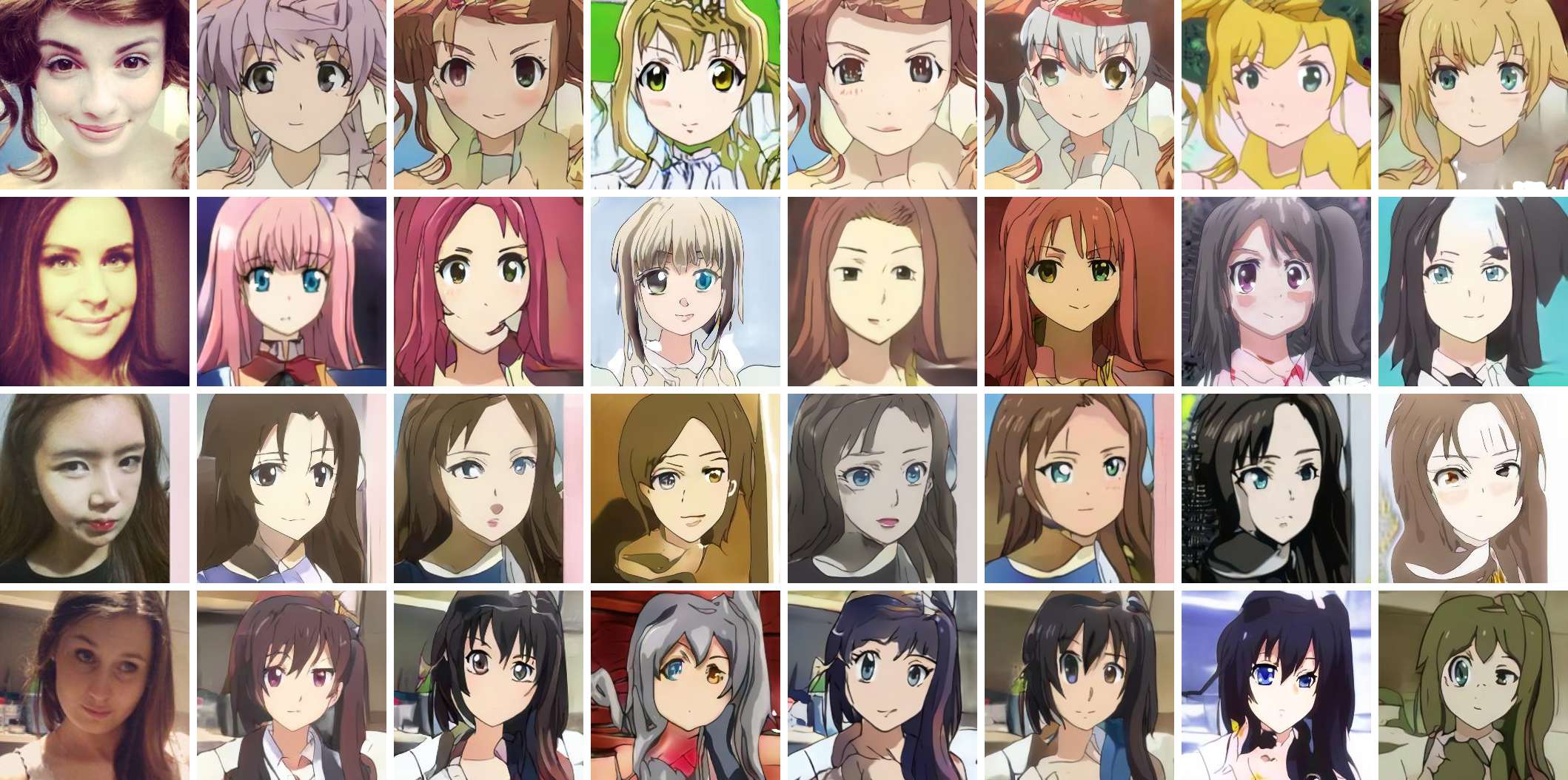
      Input         SPatchGAN       CycleGAN        MUNIT         U-GAT-IT          CUT        Council-GAN   ACL-GAN  

Figure 5: Generated images of SPatchGAN and the baselines for selfie-to-anime.

We also take a closer look at the individual outputs of SPatchGAN. The outputs of the lowest level (scale 1) and the highest level (scale 4) are shown in Figure 4 for the generated images. The outputs of the intermediate levels are in between these two. A low output value means that the discriminator can successfully distinguish the generated images from the real images, while an output near 0.5 means that the generated and real images are indistinguishable.

For a given statistical feature, the output value is larger at a lower level. This is aligned with our expectation that it is easier to match the statistical features at the low levels. The outputs at the highest level are much smaller than 0.5, and are consistent with the FID and KID results that there is still some difference between the generated and the real images. The outputs for the channel-wise max feature are below the other two features. This is due to its nature of focusing on the most discriminative patch for each feature channel. It is also worth noting that the channel-wise standard deviation feature is slightly more discriminative than the channel-wise mean feature at the highest level. It implies the importance of considering the relation among patches. In contrast, it is much more difficult for the individual patch based method to be aware of the inter-patch relations.

4.3 Comparison with Baseline

We compare SPatchGAN to the baselines, and summarize the quantitative results in Table 2. The qualitative results are shown in Figure 5, Figure 6 and Figure 7.

Selfie-to-Anime. Selfie to anime is an application that requires significant shape and texture change. The generated images are shown in Figure 5. Our method generally achieves the desirable shape deformation, e.g., the anime-style bangs, the reduced height of the face, and two enlarged eyes with roughly the same size. In contrast, other methods often cause incomplete hairstyle change, inconsistent sizes or color of the two eyes, and oversimplified texture. Our method outperforms all the baselines in term of FID and KID in Table 2. The improved image structure of our method comes from the global view of the statistical features, and the relaxed constraints on the generator.

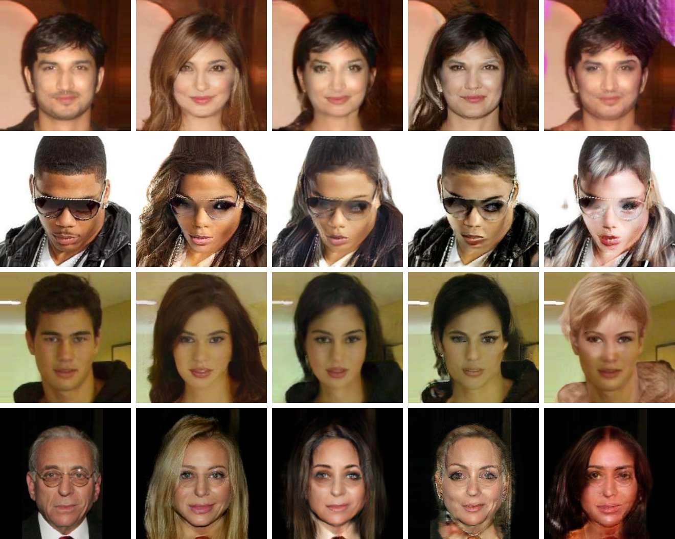
    Input        SPatchGAN     U-GAT-IT     Council-GAN   ACL-GAN

Figure 6: Generated images of SPatchGAN and the baselines for male-to-female.

Male-to-Female. To translate a male face to a female face, the major challenge is to change the hairstyle. Some minor modification are also needed for other parts such as the skin and the lips. The generated images are shown in Figure 6. Similar to the selfie-to-anime application, our model does a better job than other models for changing the hairstyle, showcasing the outstanding capability for shape deformation. Our model also manages to remove the beard, smooth the skin and color the lips naturally. The improved local details show the effectiveness of feature matching at the low levels. We achieve much better quantitative results than the baselines according to Table 2.

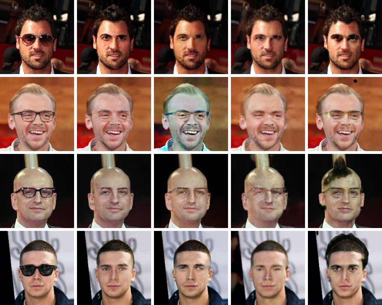
    Input        SPatchGAN     U-GAT-IT     Council-GAN   ACL-GAN

Figure 7: Generated images of SPatchGAN and the baselines for glasses removal.

Glasses Removal. Different from the aforementioned two applications, we expect to change only a small area of the image for glasses removal. The generated images are shown in Figure 7. Our method generally has less traces of the glasses on the generated images. This is mainly due to the relaxed cycle constraints. Our model is less likely to generate collapsed eyes for the inputs with sunglasses, thanks to the improved stability. Furthermore, we often observe undesirable changes outside the area of glasses with the baselines. Though we have relaxed the cycle constraints, we can still suppress the redundant changes with the weak cycle loss and the identity loss. Again, our model achieves the best FID and KID in Table 2.

5 Conclusions

In this paper, we have proposed an SPatchGAN discriminator for unsupervised image translation. Our discriminator stabilizes the network by statistical feature matching at multiple scales. It also enables training with relaxed constraints. We have shown in the experiments that our method improves the quality of the generated images, especially those with a large shape deformation. Our model outperforms the existing methods on both FID and KID metrics.

Acknowledgments. We would like to thank Kang Chen and Kewei Yang for helpful discussions.

6 Supplementary Material

In this document, we provide the detailed network architecture of SPatchGAN, the data augmentation method, the study about the weak cycle constraint, the experimental results of applying the SPatchGAN discriminator to other image translation frameworks, as well as additional comparison results for SPatchGAN and the baselines.

6.1 Implementation Details

We describe the details of our network architecture in this section. A convolutional layer with kernel size $p\times p$, stride $q$ and number of output channels $w$ is denoted as K$p$-S$q$-C$w$. A fully connected layer with number of output channels $w$ is denoted as FC$w$. A $2\times$ nearest-neighbor upsampling layer is denoted as U2. A residual block with a shortcut branch and a residual branch $b$ is denoted as RES($b$). A block $b$ repeated $z$ times is denoted as $b\times z$.

Discriminator. The discriminator consists of a feature extraction block and four scales. Each scale has a downsampling block, an adaptation block and three MLPs. Spectral normalization (SN) and Leaky-ReLU (LReLU) with a slope of 0.2 are used in the discriminator.

• Feature extraction block: K4-S2-C256-SN-LReLU, K4-S2-C512-SN-LReLU.

• Downsampling block: K4-S2-C1024-SN-LReLU.

• Adaptation block: (K1-S1-C1024-SN-LReLU) $\times 2$.

• MLP: (FC1024-SN-LReLU) $\times 2$, FC1-SN.

Given an input tensor $a\in\mathbb{R}^{H\times W\times C}$ with height $H$, width $W$ and number of channels $C$, the statistical feature of uncorrected standard deviation is calculated as

$$s_{k}=\sqrt{\frac{1}{HW}\sum_{i=1}^{H}\sum_{j=1}^{W}{(a_{i,j,k}-\bar{a_{k}})^{2}}},$$ (10)

where $s_{k}$ is the $k$-th element of the output feature vector $s\in\mathbb{R}^{C}$, $\bar{a_{k}}$ is the average value of the $k$-th input feature map, and $a_{i,j,k}$ is the input element at the $i$-th row, $j$-th column of the $k$-th feature map.

Forward generator. The forward generator consists of a downsampling module, a residual module, and an upsampling module. We use instance normalization (IN) in the downsampling and residual modules, and use layer normalization (LN) in the upsampling module. ReLU is utilized as the activation function except for the output layer, which uses Tanh.

• Downsampling module: K3-S2-C128-IN-ReLU, K3-S2-C256-IN-ReLU, K3-S2-C512-IN-ReLU.

• Residual module: RES(K3-S1-C512-IN-ReLU, K3-S1-C512-IN) $\times 8$.

• Upsampling module: U2, (K3-S1-C512-LN-ReLU) $\times 2$, U2, K3-S1-C256-LN-ReLU, U2, K3-S1-C128-LN-ReLU, K3-S1-C3-Tanh.

Backward generator. The backward generator has a pre-mixing module, a residual module, and a post-mixing module. The residual module has the same structure as the forward generator.

• Pre-mixing module: K3-S1-C512-IN.

• Post-mixing module: K3-S1-C512-LN-ReLU, K3-S1-C3-Tanh.

6.2 Data Augmentation

For selfie-to-anime, we adopt the data augmentation method in U-GAT-IT that first resizes the images to $286\times 286$, then randomly crops the images to $256\times 256$. For male-to-female and glasses removal, the images are center cropped to $178\times 178$, resized to $256\times 256$, and randomly shifted by up to $13$ pixels horizontally and vertically.

We apply color jittering with random brightness offset in $[-0.125,0.125]$, random hue offset in $[-0.02,0.02]$, random saturation factor in $[0.8,1.2]$, and random contrast factor in $[0.8,1.2]$. All images are also randomly flipped horizontally.

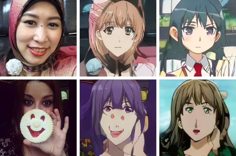
     Input           w/ Cycle        w/o Cycle    

(a) Selfie-to-anime

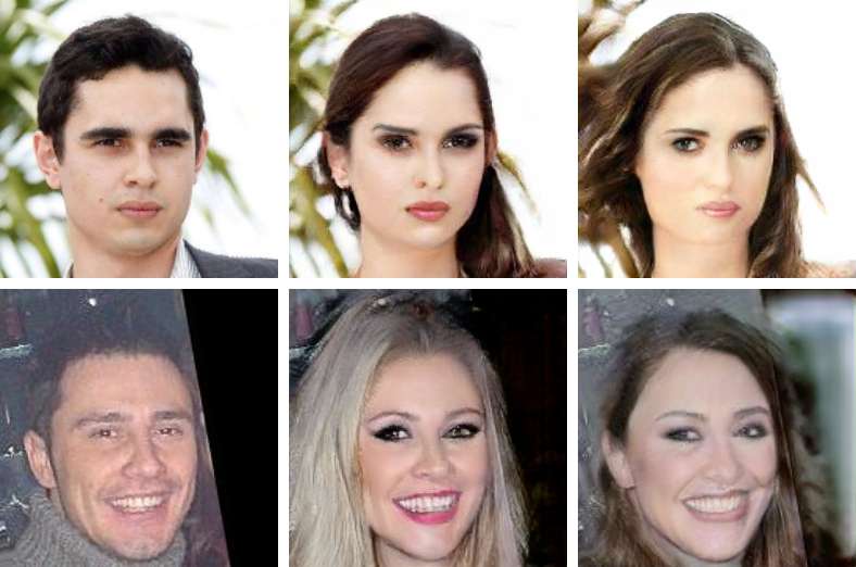
     Input           w/ Cycle        w/o Cycle    

(b) Male-to-female

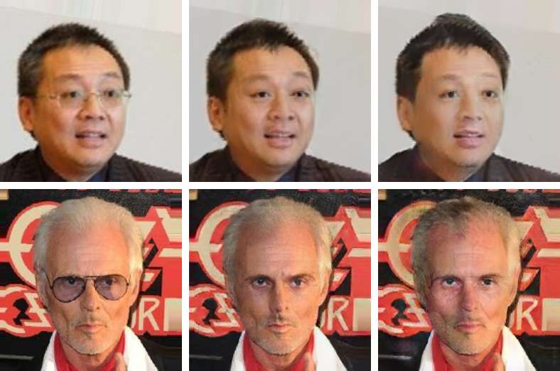
     Input           w/ Cycle        w/o Cycle    

(c) Glasses removal

Figure 8: Generated images of SPatchGAN with and without the weak cycle constraint. Some redundant changes can be observed after removing the weak cycle constraint.

Model	Selfie-to-Anime		Male-to-Female		Glasses Removal
	FID	KID	FID	KID	FID	KID
SPatchGAN w/ Weak Cycle	83.3	0.0214	8.73	0.0056	13.9	0.0031
SPatchGAN w/o Weak Cycle	82.4	0.0168	11.4	0.0080	16.2	0.0047

Table 3: Quantitative results of SPatchGAN with and without the weak cycle constraint. Lower is better.

6.3 Study of the Weak Cycle Constraint

To further evaluate the stability of SPatchGAN, we try to completely remove the weak cycle constraint. The qualitative results are shown in Figure 8. The generated images still have a good overall quality, verifying that the network has been stabilized to a large extent by the discriminator itself. However, the results without the weak cycle sometimes become too disconnected from the source images. E.g., the headscarf and the object in front of the face completely disappear in Figure 8(a). There are also some undesirable changes of the background in Figure 8(b), and some redundant changes of the hair in Figure 8(c).

The quantitative results are summarized in Table 3. The FID and KID actually improve for selfie-to-anime after removing the weak cycle. This is partially due to the fact that the similarity between the source and generated images is not considered by the metrics. Without the constraint, the images can be translated more freely to match the distributions. We enable the weak cycle in the default setting, since it is desirable to keep the generated image correlated to the source image.

The weak cycle is beneficial for FID and KID in the male-to-female and glasses removal cases. For the applications which aim to adjust only a part of the image, the constraint helps to exclude the unnecessary changes and make the training process more efficient.

Generally speaking, our method helps to separate the need for keeping the source and target images correlated from the need for stabilizing the network. The former is ensured by the weak cycle constraint, while the latter is mainly guaranteed by the SPatchGAN discriminator. Therefore, we can optimize the cycle weight $\lambda^{cyc}$ on an application basis without worrying too much about the stability issues. In contrast, the flexibility of the original cycle based framework is much more limited, since the cycle constraints have to be strict enough to stabilize the network.

6.4 Applicability to Other Frameworks

The SPatchGAN discriminator is generally agnostic of the architecture and constraints for the generator, and can be potentially leveraged to enhance other image translation frameworks. To study its applicability to other frameworks, we directly replace the default discriminators of CycleGAN and MUNIT with the discriminator of SPatchGAN, and evaluate their performance with the male-to-female dataset. The other modules and hyperparameters are unchanged. The qualitative and quantitative results are shown in Figure 9 and Table 4. CycleGAN and MUNIT with the SPatchGAN discriminator are denoted as S-CycleGAN and S-MUNIT respectively. Multimodal results are shown for MUNIT and S-MUNIT.

With the full cycle constraints, the main problem of CycleGAN is the limited shape deformation. In contrast, MUNIT introduces additional stochasticity for multimodality, and suffers more from the instability issue. It can be seen from Figure 9 that S-CycleGAN helps to make the hairstyle and face more feminine than CycleGAN. S-MUNIT helps to alleviate the blurriness of the generated images compared to MUNIT. The quantitative results of S-CycleGAN and S-MUNIT are also better than CycleGAN and MUNIT according to Table 4.

Model	FID	KID
CycleGAN	24.5	0.0240
S-CycleGAN	13.4	0.0107
MUNIT	20.8	0.0161
S-MUNIT	17.0	0.0123

Table 4: Quantitative results of the applicability studies for male-to-female. Lower is better.

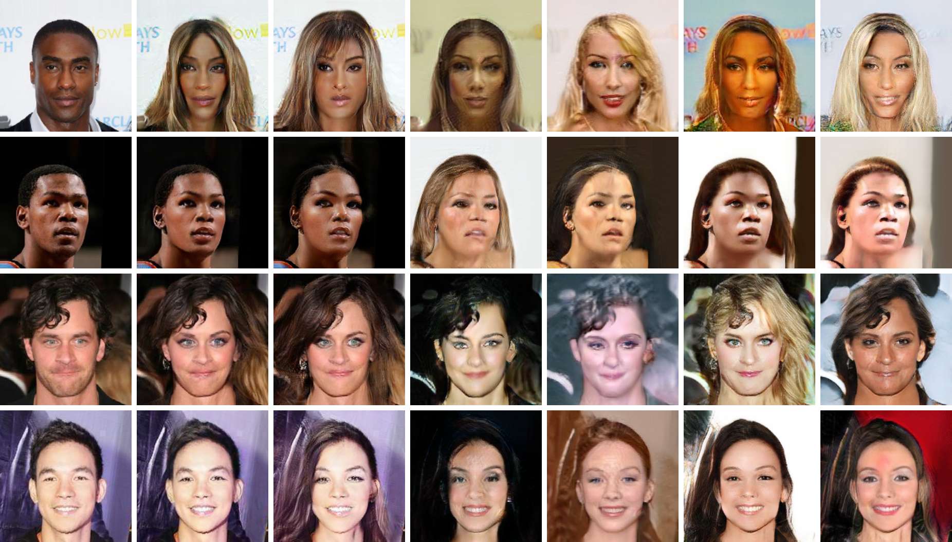
          Input            CycleGAN        S-CycleGAN        MUNIT-1          MUNIT-2         S-MUNIT-1        S-MUNIT-2      

Figure 9: Generated images of the applicability studies for male-to-female.

6.5 Additional Experimental Results

We show additional results for selfie-to-anime, male-to-female and glasses removal in Figure 10, Figure 11 and Figure 12, respectively.

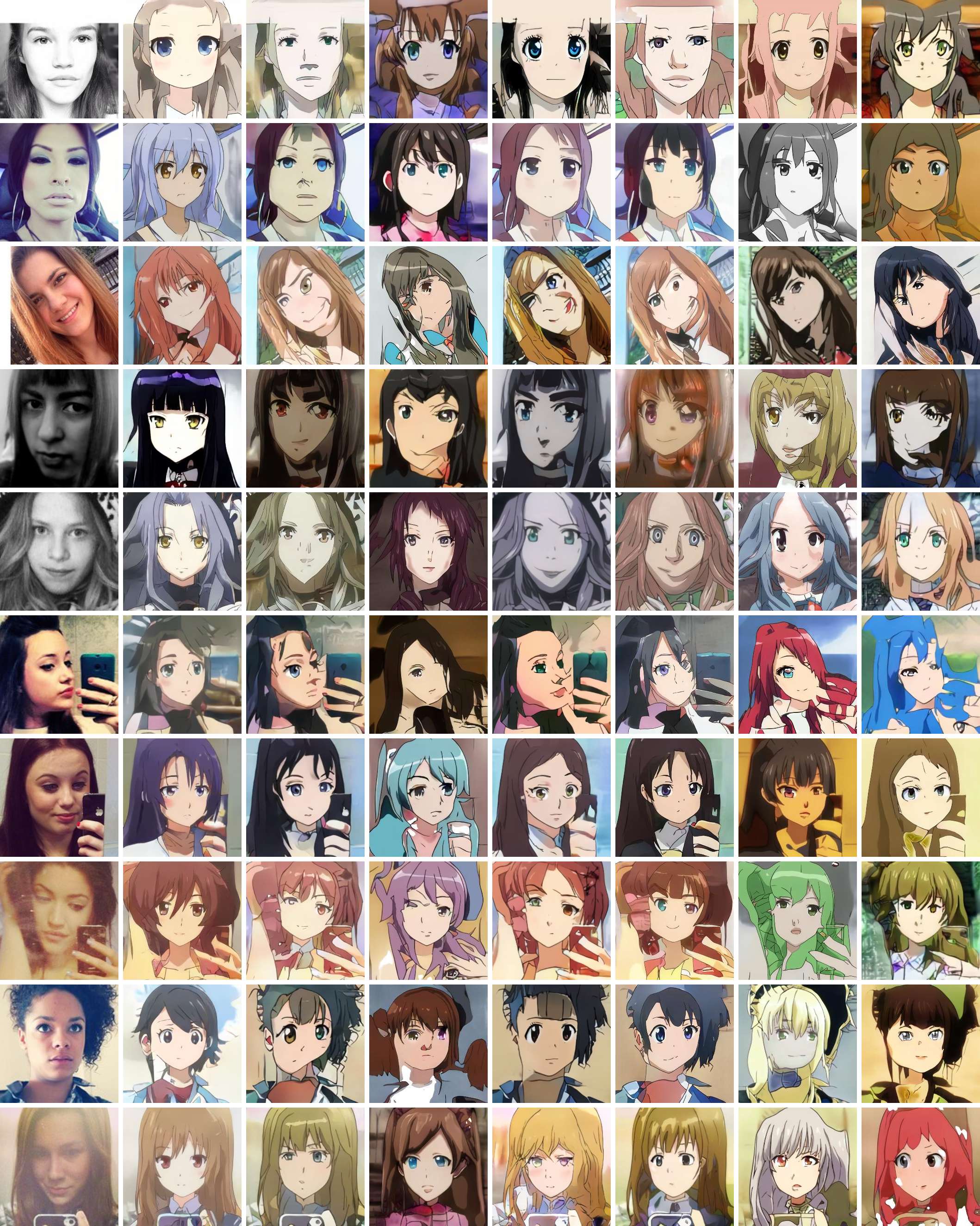
      Input            SPatchGAN       CycleGAN          MUNIT           U-GAT-IT             CUT           Council-GAN      ACL-GAN  

Figure 10: Additional results of selfie-to-anime translation.

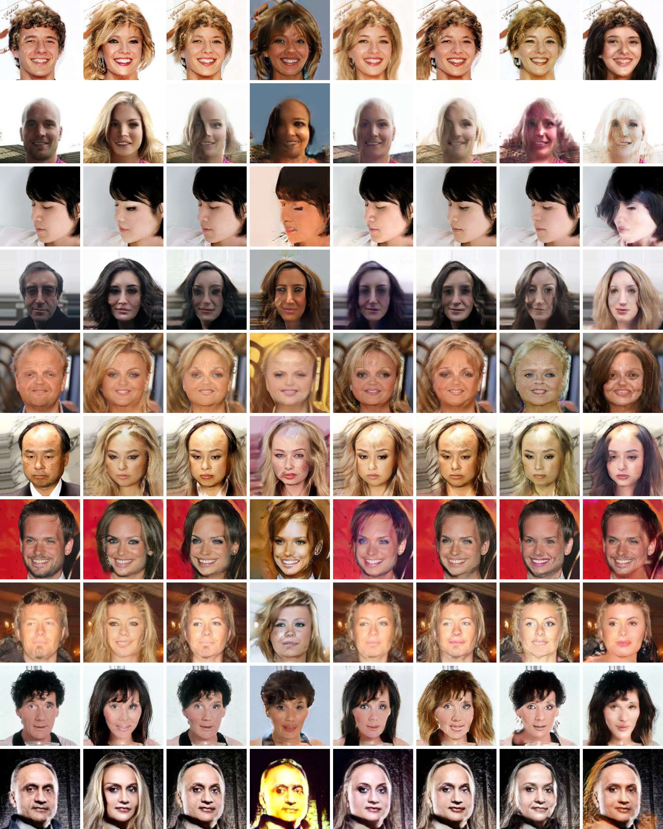
      Input            SPatchGAN       CycleGAN          MUNIT           U-GAT-IT             CUT           Council-GAN      ACL-GAN  

Figure 11: Additional results of male-to-female translation.

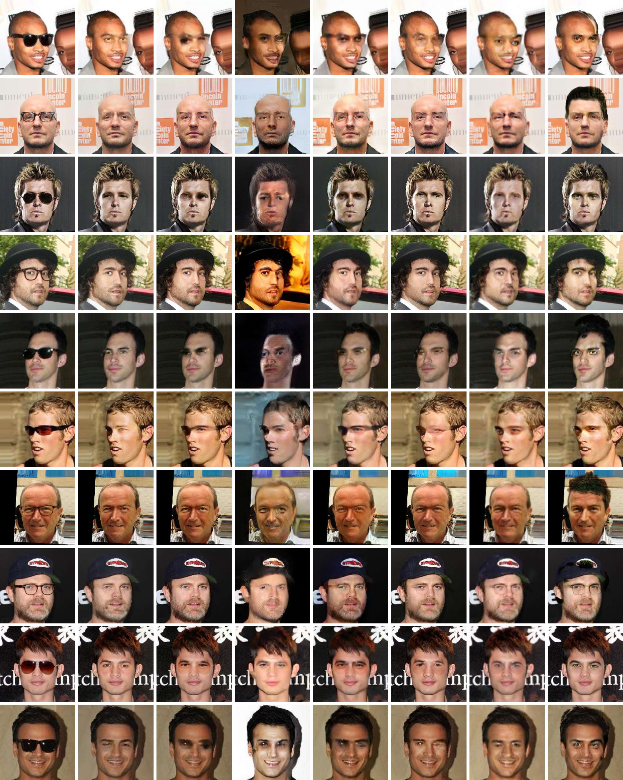
      Input            SPatchGAN       CycleGAN          MUNIT           U-GAT-IT             CUT           Council-GAN      ACL-GAN  

Figure 12: Additional results of glasses removal.

References

- [1] Amjad Almahairi, Sai Rajeswar, Alessandro Sordoni, Philip Bachman, and Aaron C. Courville. Augmented cyclegan: Learning many-to-many mappings from unpaired data. In Proceedings of the 35th International Conference on Machine Learning, ICML 2018, Stockholmsmässan, Stockholm, Sweden, July 10-15, 2018, volume 80, pages 195–204, 2018.
- [2] Martín Arjovsky, Soumith Chintala, and Léon Bottou. Wasserstein GAN. CoRR, abs/1701.07875, 2017.
- [3] Lei Jimmy Ba, Jamie Ryan Kiros, and Geoffrey E. Hinton. Layer normalization. CoRR, abs/1607.06450, 2016.
- [4] Mikolaj Binkowski, Danica J. Sutherland, Michael Arbel, and Arthur Gretton. Demystifying MMD gans. In 6th International Conference on Learning Representations, ICLR 2018, Vancouver, BC, Canada, April 30 - May 3, 2018, Conference Track Proceedings, 2018.
- [5] Andrew Brock, Jeff Donahue, and Karen Simonyan. Large scale GAN training for high fidelity natural image synthesis. In 7th International Conference on Learning Representations, ICLR 2019, New Orleans, LA, USA, May 6-9, 2019, 2019.
- [6] Yang Chen, Yu-Kun Lai, and Yong-Jin Liu. Cartoongan: Generative adversarial networks for photo cartoonization. In 2018 IEEE Conference on Computer Vision and Pattern Recognition, CVPR 2018, Salt Lake City, UT, USA, June 18-22, 2018, pages 9465–9474, 2018.
- [7] Ian J. Goodfellow, Jean Pouget-Abadie, Mehdi Mirza, Bing Xu, David Warde-Farley, Sherjil Ozair, Aaron C. Courville, and Yoshua Bengio. Generative adversarial nets. In Advances in Neural Information Processing Systems 27: Annual Conference on Neural Information Processing Systems 2014, December 8-13 2014, Montreal, Quebec, Canada, pages 2672–2680, 2014.
- [8] Ishaan Gulrajani, Faruk Ahmed, Martín Arjovsky, Vincent Dumoulin, and Aaron C. Courville. Improved training of wasserstein gans. In Advances in Neural Information Processing Systems 30: Annual Conference on Neural Information Processing Systems 2017, December 4-9, 2017, Long Beach, CA, USA, pages 5767–5777, 2017.
- [9] Martin Heusel, Hubert Ramsauer, Thomas Unterthiner, Bernhard Nessler, and Sepp Hochreiter. Gans trained by a two time-scale update rule converge to a local nash equilibrium. In Advances in Neural Information Processing Systems 30: Annual Conference on Neural Information Processing Systems 2017, December 4-9, 2017, Long Beach, CA, USA, pages 6626–6637, 2017.
- [10] Xun Huang, Ming-Yu Liu, Serge J. Belongie, and Jan Kautz. Multimodal unsupervised image-to-image translation. In Computer Vision - ECCV 2018 - 15th European Conference, Munich, Germany, September 8-14, 2018, Proceedings, Part III, volume 11207, pages 179–196, 2018.
- [11] Phillip Isola, Jun-Yan Zhu, Tinghui Zhou, and Alexei A. Efros. Image-to-image translation with conditional adversarial networks. In 2017 IEEE Conference on Computer Vision and Pattern Recognition, CVPR 2017, Honolulu, HI, USA, July 21-26, 2017, pages 5967–5976, 2017.
- [12] Animesh Karnewar and Oliver Wang. MSG-GAN: multi-scale gradients for generative adversarial networks. In 2020 IEEE/CVF Conference on Computer Vision and Pattern Recognition, CVPR 2020, Seattle, WA, USA, June 13-19, 2020, pages 7796–7805, 2020.
- [13] Tero Karras, Timo Aila, Samuli Laine, and Jaakko Lehtinen. Progressive growing of gans for improved quality, stability, and variation. In 6th International Conference on Learning Representations, ICLR 2018, Vancouver, BC, Canada, April 30 - May 3, 2018, Conference Track Proceedings, 2018.
- [14] Tero Karras, Samuli Laine, and Timo Aila. A style-based generator architecture for generative adversarial networks. In IEEE Conference on Computer Vision and Pattern Recognition, CVPR 2019, Long Beach, CA, USA, June 16-20, 2019, pages 4401–4410, 2019.
- [15] Tero Karras, Samuli Laine, Miika Aittala, Janne Hellsten, Jaakko Lehtinen, and Timo Aila. Analyzing and improving the image quality of stylegan. In 2020 IEEE/CVF Conference on Computer Vision and Pattern Recognition, CVPR 2020, Seattle, WA, USA, June 13-19, 2020, pages 8107–8116, 2020.
- [16] Junho Kim, Minjae Kim, Hyeonwoo Kang, and Kwanghee Lee. U-GAT-IT: unsupervised generative attentional networks with adaptive layer-instance normalization for image-to-image translation. In 8th International Conference on Learning Representations, ICLR 2020, Addis Ababa, Ethiopia, April 26-30, 2020, 2020.
- [17] Taeksoo Kim, Moonsu Cha, Hyunsoo Kim, Jung Kwon Lee, and Jiwon Kim. Learning to discover cross-domain relations with generative adversarial networks. In Proceedings of the 34th International Conference on Machine Learning, ICML 2017, Sydney, NSW, Australia, 6-11 August 2017, volume 70, pages 1857–1865, 2017.
- [18] Diederik P. Kingma and Jimmy Ba. Adam: A method for stochastic optimization. In 3rd International Conference on Learning Representations, ICLR 2015, San Diego, CA, USA, May 7-9, 2015, Conference Track Proceedings, 2015.
- [19] Hsin-Ying Lee, Hung-Yu Tseng, Qi Mao, Jia-Bin Huang, Yu-Ding Lu, Maneesh Singh, and Ming-Hsuan Yang. DRIT++: diverse image-to-image translation via disentangled representations. Int. J. Comput. Vis., 128(10):2402–2417, 2020.
- [20] Ming-Yu Liu, Thomas Breuel, and Jan Kautz. Unsupervised image-to-image translation networks. In Advances in Neural Information Processing Systems 30: Annual Conference on Neural Information Processing Systems 2017, December 4-9, 2017, Long Beach, CA, USA, pages 700–708, 2017.
- [21] Ziwei Liu, Ping Luo, Xiaogang Wang, and Xiaoou Tang. Deep learning face attributes in the wild. In 2015 IEEE International Conference on Computer Vision, ICCV 2015, Santiago, Chile, December 7-13, 2015, pages 3730–3738, 2015.
- [22] Xudong Mao, Qing Li, Haoran Xie, Raymond Y. K. Lau, Zhen Wang, and Stephen Paul Smolley. Least squares generative adversarial networks. In IEEE International Conference on Computer Vision, ICCV 2017, Venice, Italy, October 22-29, 2017, pages 2813–2821, 2017.
- [23] Luke Metz, Ben Poole, David Pfau, and Jascha Sohl-Dickstein. Unrolled generative adversarial networks. In 5th International Conference on Learning Representations, ICLR 2017, Toulon, France, April 24-26, 2017, Conference Track Proceedings, 2017.
- [24] Mehdi Mirza and Simon Osindero. Conditional generative adversarial nets. CoRR, abs/1411.1784, 2014.
- [25] Takeru Miyato, Toshiki Kataoka, Masanori Koyama, and Yuichi Yoshida. Spectral normalization for generative adversarial networks. In 6th International Conference on Learning Representations, ICLR 2018, Vancouver, BC, Canada, April 30 - May 3, 2018, Conference Track Proceedings, 2018.
- [26] Ori Nizan and Ayellet Tal. Breaking the cycle - colleagues are all you need. In 2020 IEEE/CVF Conference on Computer Vision and Pattern Recognition, CVPR 2020, Seattle, WA, USA, June 13-19, 2020, pages 7857–7866, 2020.
- [27] Taesung Park, Alexei A. Efros, Richard Zhang, and Jun-Yan Zhu. Contrastive learning for unpaired image-to-image translation. In Computer Vision - ECCV 2020 - 16th European Conference, Glasgow, UK, August 23-28, 2020, Proceedings, Part IX, volume 12354, pages 319–345, 2020.
- [28] Alec Radford, Luke Metz, and Soumith Chintala. Unsupervised representation learning with deep convolutional generative adversarial networks. In 4th International Conference on Learning Representations, ICLR 2016, San Juan, Puerto Rico, May 2-4, 2016, Conference Track Proceedings, 2016.
- [29] Tim Salimans, Ian J. Goodfellow, Wojciech Zaremba, Vicki Cheung, Alec Radford, and Xi Chen. Improved techniques for training gans. In Advances in Neural Information Processing Systems 29: Annual Conference on Neural Information Processing Systems 2016, December 5-10, 2016, Barcelona, Spain, pages 2226–2234, 2016.
- [30] Md Mahfuzur Rahman Siddiquee, Zongwei Zhou, Nima Tajbakhsh, Ruibin Feng, Michael B. Gotway, Yoshua Bengio, and Jianming Liang. Learning fixed points in generative adversarial networks: From image-to-image translation to disease detection and localization. In 2019 IEEE/CVF International Conference on Computer Vision, ICCV 2019, Seoul, Korea (South), October 27 - November 2, 2019, pages 191–200, 2019.
- [31] Yaniv Taigman, Adam Polyak, and Lior Wolf. Unsupervised cross-domain image generation. In 5th International Conference on Learning Representations, ICLR 2017, Toulon, France, April 24-26, 2017, Conference Track Proceedings, 2017.
- [32] Dmitry Ulyanov, Andrea Vedaldi, and Victor S. Lempitsky. Improved texture networks: Maximizing quality and diversity in feed-forward stylization and texture synthesis. In 2017 IEEE Conference on Computer Vision and Pattern Recognition, CVPR 2017, Honolulu, HI, USA, July 21-26, 2017, pages 4105–4113, 2017.
- [33] Ting-Chun Wang, Ming-Yu Liu, Jun-Yan Zhu, Andrew Tao, Jan Kautz, and Bryan Catanzaro. High-resolution image synthesis and semantic manipulation with conditional gans. In 2018 IEEE Conference on Computer Vision and Pattern Recognition, CVPR 2018, Salt Lake City, UT, USA, June 18-22, 2018, pages 8798–8807, 2018.
- [34] Han Zhang, Ian J. Goodfellow, Dimitris N. Metaxas, and Augustus Odena. Self-attention generative adversarial networks. In Proceedings of the 36th International Conference on Machine Learning, ICML 2019, 9-15 June 2019, Long Beach, California, USA, volume 97, pages 7354–7363, 2019.
- [35] Yihao Zhao, Ruihai Wu, and Hao Dong. Unpaired image-to-image translation using adversarial consistency loss. In Computer Vision - ECCV 2020 - 16th European Conference, Glasgow, UK, August 23-28, 2020, Proceedings, Part IX, volume 12354, pages 800–815, 2020.
- [36] Bolei Zhou, Aditya Khosla, Àgata Lapedriza, Aude Oliva, and Antonio Torralba. Learning deep features for discriminative localization. In 2016 IEEE Conference on Computer Vision and Pattern Recognition, CVPR 2016, Las Vegas, NV, USA, June 27-30, 2016, pages 2921–2929, 2016.
- [37] Jun-Yan Zhu, Taesung Park, Phillip Isola, and Alexei A. Efros. Unpaired image-to-image translation using cycle-consistent adversarial networks. In IEEE International Conference on Computer Vision, ICCV 2017, Venice, Italy, October 22-29, 2017, pages 2242–2251, 2017.