First-order Bose-Einstein condensation with three-body interacting bosons

Abstract

Bose-Einstein condensation, observed in either strongly interacting liquid helium or weakly interacting atomic Bose gases, is widely known to be a second-order phase transition. Here, we predict a first-order Bose-Einstein condensation in a cloud of harmonically trapped bosons interacting with both attractive two-body interaction and repulsive three-body interaction, characterized respectively by an $s$-wave scattering length $a<0$ and a three-body scattering hypervolume $D>0$. It happens when the harmonic trapping potential is weak, so with increasing temperature the system changes from a low-temperature liquid-like quantum droplet to a normal gas, and therefore experiences a first-order liquid-to-gas transition. At large trapping potential, however, the quantum droplet can first turn into a superfluid gas, rendering the condensation transition occurred later from a superfluid gas to a normal gas smooth. We determine a rich phase diagram and show the existence of a tri-critical point, where the three phases - quantum droplet, superfluid gas and normal gas - meet together. We argue that an ensemble of spin-polarized tritium atoms could be a promising candidate to observe the predicted first-order Bose-Einstein condensation, across which the condensate fraction or central condensate density jumps to zero and the surface-mode frequencies diverge.

Bose-Einstein condensation (BEC) is a ubiquitous quantum phenomenon that occurs in a wide range of many-body systems, including liquid helium Griffin1993 , atomic Bose gases Anderson1995 ; Dalfovo1999 , conventional and high-temperature superconductors Lee2006 , and even the hypothetical dark matter axions Sikivie2009 . All the BEC transitions observed so far are of second-order and are described by the model $F$ in the $XY$ universality class with $O(2)$ symmetry Hohenberg1977 . In strongly interacting liquid helium, it is a continuous transition from a normal liquid (He-I) to a superfluid liquid (He-II) across the $\lambda$-line Griffin1993 ; while in weakly interacting gaseous Bose systems of ⁸⁷Rb atoms Anderson1995 ; Dalfovo1999 , it is a smooth transition from a normal gas to a superfluid gas.

In this Letter, we propose that a first-order BEC transition from a superfluid liquid to a normal gas could occur in weakly interacting atomic Bose gases, when the two-body interaction is tuned to be attractive (i.e., the $s$-wave scattering length $a<0$) and the resulting mean-field collapse is arrested by a repulsive three-body interaction characterized by the scattering hypervolume $D>0$. Our proposal is motivated by the recent experimental realizations of liquid-like quantum droplets Bottcher2021 in dipolar Bose-Einstein condensates FerrierBarbut2016 ; Schmitt2016 ; Chomaz2016 or two-component Bose-Bose mixtures with attractive inter-species interactions Cabrera2018 ; Semeghini2018 ; DErrico2019 , which may experience a liquid-to-gas transition at nonzero temperature. However, a careful examination of the temperature effect Wang2020a ; Wang2020b indicates that the Lee-Huang-Yang (LHY) quantum fluctuation, which is the key ingredient of the droplet formation Petrov2015 ; Minardi2019 ; Hu2020a ; Hu2020b ; Gu2020 ; Zin2021 ; Cui2021 ; Pan2021 , is too fragile to finite temperature. As a result, LHY droplets are thermally destabilized far below the superfluid transition Wang2020a ; Wang2020b . To overcome such a thermal instability, we resort to earlier cold-atom proposals for quantum droplets based on the three-body repulsive interactions Gammal2000 ; Bulgac2002 ; Blume2002 ; Gao2004 ; Beslic2009 , which play the same role as LHY quantum fluctuations but are less sensitive to temperature. These proposals regain considerable interest mostly recently Zwerger2019 ; Mestrom2020 , owing to the brilliant idea by Shina Tan and his co-worker that non-trivial three-body effects can be expressed in terms of a single parameter of the hypervolume $D$ Tan2008 , which can become positive and significant near the zero-crossing of the two-body scattering length $a$ Zhu2017 . Quantum droplets supported by the three-body interactions at zero temperature have then been discussed Zwerger2019 ; Mestrom2020 ; Hu2020c .

Here, we address the finite-temperature properties of three-body interacting bosons confined in three-dimensional (3D) harmonic traps, by using the standard Hartree-Fock-Bogoliubov-Popov (HFB-Popov) theory Griffin1996 ; Hutchinson1997 ; Shi1998 . At weak trapping potential, we find two phases, a low-temperature quantum droplet and a high-temperature normal gas, separated by the first-order BEC. While at large trapping potential, another superfluid gas phase emerges and replaces the droplet phase. This leads to the conventional smooth BEC transition between a superfluid gas and a normal gas. An intriguing tri-critical point is formed in the phase diagram, at which the quantum droplet, superfluid gas and normal gas intersect. We explore the scenario of realizing such a tri-critical point with ultracold atoms, for example, using a cloud of spin-polarized tritium atoms Blume2002 ; Beslic2009 .

Incidentally, a similar tri-critical point has recently been discussed by Dam Thanh Son and his collaborators for ultra quantum liquids formed by a hypothetical isotope of helium with nuclear mass less than 4 atomic mass units Kora2020 ; Son2021 . Our results complement their studies and take the unique advantage of the unprecedented controllability and simplicity with ultracold atoms Dalfovo1999 . The liquid-to-gas transition and BEC transition have also been considered in the context of strongly-interacting matter of $\alpha$-particles Satarov2017 . Therefore, it turns out that the first-order BEC transition predicted in our work may find wide applications in diverse fields of physics, ranging from atomic, molecular and optical physics, to condensed matter physics, and to high-energy particle physics and nuclear physics.

Model Hamiltonian. — Three-body interacting bosons of mass $M$ in 3D harmonic traps under consideration can be well described by the model Hamiltonian, $\hat{H}=\int d\mathbf{r}\mathcal{H}(\mathbf{r})$, with the Hamiltonian density,

$$\mathcal{H}=\hat{\psi}^{\dagger}\left[-\frac{\hbar^{2}\nabla^{2}}{2M}+V_{T}-\mu\right]\hat{\psi}+\frac{g}{2}\hat{\psi}^{\dagger 2}\hat{\psi}^{2}+\frac{G}{6}\hat{\psi}^{\dagger 3}\hat{\psi}^{3}.$$ (1)

Here, $\hat{\psi}(\mathbf{r})$ and $\hat{\psi}^{\dagger}(\mathbf{r})$ are respectively annihilation and creation field operators of bosons, $\mu$ is the chemical potential to be fixed by the total number of atoms $N$, $g\equiv 4\pi\hbar^{2}a/M<0$ and $G\equiv\hbar^{2}D/M>0$ are the attractive two-body and repulsive three-body interaction strengths, respectively. The harmonic trapping potential $V_{T}(\mathbf{r})\equiv M\omega^{2}r^{2}/2$ is necessary, to prevent the atoms from escaping in the gas-like phase or the finite-temperature self-evaporation in the droplet state Wang2020b ; Petrov2015 .

HFB-Popov theory. — The model Hamiltonian at nonzero temperature $T$ can be conveniently solved by the HFB-Popov theory Griffin1996 ; Hutchinson1997 ; Shi1998 . We decompose $\hat{\psi}(\mathbf{r},t)\equiv\Phi(\mathbf{r})+\tilde{\psi}(\mathbf{r},t)$ into a condensate wave-function $\Phi(\mathbf{r})$ and a field operator $\tilde{\psi}(\mathbf{r},t)$ for noncondensate atoms. From the equation of motion for $\hat{\psi}(\mathbf{r},t)$, we deduce within the Popov approximation SM : (i) the generalized Gross-Pitaevskii equation (GPE) for the condensate wave-function,

$$\mathcal{\hat{L}}\Phi(\mathbf{r})=\mu\Phi(\mathbf{r}),$$ (2)

where we have defined the operator,

$$\mathcal{\hat{L}}\equiv-\frac{\hbar^{2}\nabla^{2}}{2M}+V_{T}+g\left(n_{c}+2\tilde{n}\right)+G\left(\frac{n_{c}^{2}}{2}+3n_{c}\tilde{n}+3\tilde{n}^{2}\right),$$

and $n_{c}(\mathbf{r})\equiv\left|\Phi(\mathbf{r})\right|^{2}$ and $\tilde{n}(\mathbf{r})\equiv\bigl{\langle}\tilde{\psi}^{\dagger}(\mathbf{r})\tilde{\psi}(\mathbf{r})\bigr{\rangle}$ are the condensate and noncondensate densities, respectively; and (ii) the coupled HFB-Popov equations for the $\eta$-th quasi-particle wave-functions $u_{\eta}$ and $v_{\eta}$ with energy $E_{\eta}>0$,

$$\left[\begin{array}[]{cc}\hat{\mathcal{L}}-\mu+\mathcal{\hat{M}}&\mathcal{\hat{M}}\\ \mathcal{\hat{M}}&\hat{\mathcal{L}}-\mu+\mathcal{\hat{M}}\end{array}\right]\left[\begin{array}[]{c}u_{\eta}\left(\mathbf{r}\right)\\ v_{\eta}\left(\mathbf{r}\right)\end{array}\right]=E_{\eta}\left[\begin{array}[]{c}+u_{\eta}\left(\mathbf{r}\right)\\ -v_{\eta}\left(\mathbf{r}\right)\end{array}\right],$$ (3)

where the operator $\hat{\mathcal{M}}\equiv gn_{c}+G(n_{c}^{2}+3n_{c}\tilde{n}).$ Once the quasi-particle wave-functions are obtained, the noncondensate density can be calculated according to,

$$\tilde{n}\left(\mathbf{r}\right)=\tilde{n}_{\textrm{qd}}\left(\mathbf{r}\right)+\sum_{\eta}\frac{\left|u_{\eta}\left(\mathbf{r}\right)\right|^{2}+\left|v_{\eta}\mathbf{\left(r\right)}\right|^{2}}{e^{\beta E_{\eta}}-1},$$ (4)

where $\tilde{n}_{\textrm{qd}}(\mathbf{r})=\sum_{\eta}\left|v_{\eta}\mathbf{(r})\right|^{2}$ is the depletion to the condensate arising from quantum fluctuations and $\beta\equiv 1/(k_{B}T)$. In the absence of the three-body interaction, i.e., $G=0$, Eq. (2) and Eq. (3) recover the well known HFB-Popov theory of a weakly interacting Bose gas Hutchinson1997 . In the normal state ($n_{c}=0$ and the total density $n=\tilde{n}$), Eq. (3) instead describes the single-particle motion under a mean-field Hartree-Fock interaction potential $2gn+3Gn^{2}$.

The Popov approximation amounts to neglecting the anomalous correlation $\tilde{m}(\mathbf{r})\equiv\bigl{\langle}\tilde{\psi}(\mathbf{r})\tilde{\psi}(\mathbf{r})\bigr{\rangle}$, which is a higher-order effect beyond mean-field Griffin1996 ; Shi1998 . It ensures the gapless phonon spectrum in the homogeneous limit Griffin1996 , where the chemical potential is given by $\mu=g(n_{c}+2\tilde{n})+G(n_{c}^{2}/2+3n_{c}\tilde{n}+3\tilde{n}^{2})$ and hence $\mathcal{\hat{L}}_{k=0}=\mu$. However, it is worth noting that, at low temperature the anomalous correlation is at the same order as the quantum depletion in magnitude. For consistency, therefore, we neglect the quantum depletion in the noncondensate density. This treatment is reasonable, since the quantum depletion is typical about ten percent SM and its absence recovers the standard GPE for condensate wave-function that has been widely adopted in the previous studies Gammal2000 ; Bulgac2002 ; Mestrom2020 ; Hu2020c . We also note that, the Popov approximation leads to an artificial first-order superfluid transition with a few percent jump in the condensate density Shi1998 . This drawback has nothing to do with the first-order BEC transition predicted in our work, where the sudden jump in the central condensate density at the transition is almost $100\%$ SM .

Numerical calculations. — We have iteratively solved Eq. (2) and Eq. (3) in a self-consistent way, with the chemical potential $\mu$ determined by the number equation $N=\int d\mathbf{r}[n_{c}(\mathbf{r})+\tilde{n}(\mathbf{r})]=N_{c}+N_{\textrm{th}}$. To ease the numerical workload, it is useful to introduce the re-scaled units for length $\mathbf{\bar{r}}\equiv\mathbf{r}/\xi$, density $\bar{n}\equiv n/n_{0}$, and energy $\bar{E}_{\eta}\equiv M\xi^{2}E_{\eta}/\hbar^{2}$, where $\xi=\sqrt{D/(6\pi^{2}a^{2})}$ is the length scale and $n_{0}=6\pi\left|a\right|/D$ is the equilibrium density of zero-temperature quantum droplets SM , so the two interaction strengths now become dimensionless: $gn_{0}M\xi^{2}/\hbar^{2}\equiv\bar{g}=-4$ and $Gn_{0}^{2}M\xi^{2}/\hbar^{2}\equiv\bar{G}=+6$. The reduced number of particles is given by $\bar{N}=N/(n_{0}\xi^{3})$ with $n_{0}\xi^{3}=\sqrt{D/6}/(\pi^{2}a^{2})$. Hereafter, without any confusion we shall remove the bar in the re-scale units.

At zero temperature, the use of the re-scaled units leads to a simple GPE equation, $[-\nabla^{2}/2+\omega^{2}r^{2}/2-4\Phi^{2}+3\Phi^{4}]\Phi=\mu\Phi$, which has been well understood Gammal2000 ; Hu2020c . For instance, without harmonic traps ($\omega=0$), the GPE allows a self-bound quantum droplet with $\Phi\simeq 1$ and $\mu\simeq-1$ for large reduced number of particles $N\gg 1$ Bulgac2002 ; Hu2020c . The droplet state is robust below a characteristic trapping frequency, i.e., $\omega\lesssim\sqrt{2}(4\pi/3N)^{1/3}\simeq 2.3N^{-1/3}$ Hu2020c . It is easy to see that, if we neglect the finite-size effect for large number of particles, the properties of the system depend on the product $N^{1/3}\omega$, as in a weakly interacting Bose gas Dalfovo1999 . Most numerical calculations in this work are therefore carried out for $N=1000$. We also vary $N$ in the range $[125,8000]$ and find no sizable finite-size effect.

In the case of quantum droplets the finite-temperature HFB-Popov equations are generally more challenging to solve than that of a weakly interacting Bose gas Hutchinson1997 . For the technical aspects of our numerical calculations, we refer to Supplemental Material for details SM .

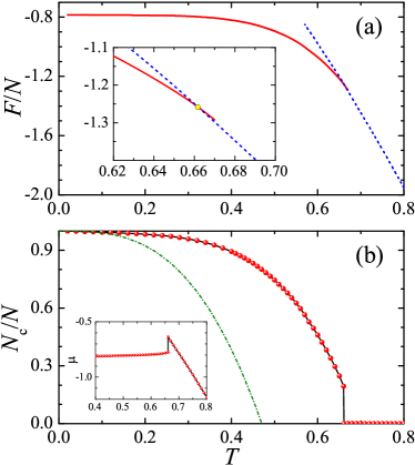
Figure 1: First-order BEC transition at $N^{1/3}\omega=0.5$. (a) Temperature dependence of the free energy for the condensed-state solution (red solid line) and for the normal-state solution (blue dashed line). The inset highlights the transition at $T_{c}\simeq 0.661$. (b) The condensate fraction as a function of temperature. The green dot-dashed line shows $N_{c}/N=1-(T/T_{c0})^{3}$, where $T_{c0}\simeq 0.9405N^{1/3}\omega$ is the transition temperature of an ideal Bose gas in harmonic traps Dalfovo1999 . The inset shows a jump in the chemical potential at $T_{c}$.

First-order BEC transition. — Let us first consider the finite-temperature thermodynamics at small effective trapping frequency, i.e., $N^{1/3}\omega=0.5$, as reported in Fig. 1. Remarkably, near the superfluid transition we always find two possible solutions: one comes with a significant condensate fraction, while the other is completely a normal state. To identify which one is the ground-state solution, we calculate the free energy $F=\Omega+\mu N$, where the thermodynamic potential $\Omega$ takes the form SM ,

$$\Omega = \sum_{\eta}\frac{\ln\left[1-e^{-\beta E_{\eta}}\right]}{\beta}+\int d\mathbf{r}\Phi^{*}\left[-\frac{\hbar^{2}\nabla^{2}}{2M}+V_{T}-\mu\right]\Phi$$ (5)

$$+\int d\mathbf{r}\left[\frac{gn_{c}^{2}}{2}-g\tilde{n}^{2}+G\left(\frac{n_{c}^{3}}{6}-3n_{c}\tilde{n}^{2}-2\tilde{n}^{3}\right)\right].$$

It is readily seen from Fig. 1(a), the free energies of the two solutions intersect at $T_{c}\simeq 0.661$ with different slope, clearly indicating a first-order BEC transition. Consequently, the condensate fraction suddenly drops to zero at $T_{c}$, as shown in Fig. 1(b). It is also significantly larger than the ideal gas result for non-interacting bosons in harmonic traps, i.e., $N_{c}/N=1-(T/T_{c0})^{3}$, where $T_{c0}=\omega[N/\zeta(3)]^{1/3}$ with the Zeta function $\zeta(3)\simeq 1.202$ Dalfovo1999 . We find that with increasing temperature the non-condensate fraction increases exponentially slowly, compared with the usual power-law $T^{3}$ behavior in the gas-like phase. This slow increase is due to the discrete excitation spectrum of the self-bound quantum droplet, which persists even in the absence of the trapping potential Hu2020c . We note that, the sudden disappearance of the condensate fraction is correlated with a jump in the chemical potential, as plotted in the inset of Fig. 1(b). The observation of a first-order BEC transition at small trapping frequency is the main result of our work.

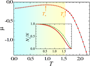
Figure 2: Second-order BEC transition at $N^{1/3}\omega=2.0$. The chemical potential is plotted as a function of temperature. It is a smooth function and the BEC transition occurs at $T_{c}\simeq 1.563$. The inset shows the condensate fraction and the green dot-dashed line is the ideal gas prediction, $N_{c}/N=1-(T/T_{c0})^{3}$.

At large trapping frequency, the situation dramatically changes. A typical case of $N^{1/3}\omega=2.0$ is presented in Fig. 2. Both chemical potential and condensate fraction change smoothly when temperature increases, suggesting a second-order superfluid phase transition. We interpret it as a transition from a superfluid gas to a normal gas, and therefore use the standard approach to determine a critical temperature $T_{c}\simeq 1.563$, at which the condensate fraction should change most significantly (i.e., $d^{2}N_{c}/dT^{2}=0$) Hu2003 . Our interpretation follows the two observations that the chemical potential is a decreasing function of temperature near the superfluid transition and the condensate fraction lies systematically below the ideal gas prediction (i.e., the green dot-dashed line), both of which are the key features of the second-order transition of a weakly interacting Bose gas Dalfovo1999 . Interestingly, at low temperature the chemical potential is rather an increasing function of temperature up to a turning point (indicated by $T_{*}\simeq 1.0$ in the figure), which is consistent with the picture of a quantum droplet muQuantumDroplet . Thus, the system seems to cross from a liquid-like droplet over to a gas-like phase at the characteristic temperature $T_{*}$.

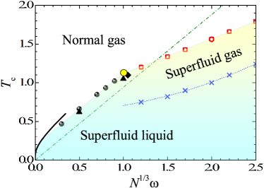
Figure 3: Critical temperature $T_{c}$ (closed and open symbols) and crossover temperature $T_{*}$ (crosses) as a function of $N^{1/3}\omega$. The thick solid line is the critical temperature predicted at small trapping frequency, i.e., $N^{1/3}\omega=T_{c}\exp\left[-1/(3T_{c})\right]$. The green dot-dashed line shows $T_{c0}\simeq 0.9405N^{1/3}\omega$. The dotted line that connects the crossover temperature $T_{*}$ is the guide for the eye. A tri-critical point is highlighted by the yellow dot. Typically, we take $N=1000$. The change in the reduced number of particles (i.e., the triangles for $N=125$ and diamonds for $N=3375$ and hexagons for $N=8000$) does not lead to sizable difference to $T_{c}$.

Phase diagram. — By calculating the critical temperature $T_{c}$ and crossover temperature $T_{*}$ at different effective trapping frequency $N^{1/3}\omega$, we determine a phase diagram in Fig. 3. An intriguing tri-critical point appears at $(N^{1/3}\omega)_{\textrm{tri}}\simeq 1.0$ and $T_{\textrm{tri}}\simeq 1.13$, where the droplet phase (i.e., superfluid liquid), superfluid gas and normal gas intersect with others. Below the tri-critical trapping frequency, i.e., $N^{1/3}\omega<1.0$, a superfluid liquid turns into a normal gas via a first-order transition (black solid symbols); while at $N^{1/3}\omega>1.0$, with increasing temperature the superfluid liquid first becomes a superfluid gas at the crossover temperature $T_{*}$ (crosses) and then turns into a normal gas via a smooth second-order phase transition (red empty symbols). Note that, with decreasing $N^{1/3}\omega$ the crossover temperature $T_{*}$ does not converge to the tri-critical point. This is probably due to the difficulty of defining an appropriate crossover temperature in a finite-size system close to the tri-critical point SM .

At vanishingly small trapping frequency (i.e., $N^{1/3}\omega\rightarrow 0$), the critical temperature can be analytically derived SM . We find that the relation $N^{1/3}\omega=T_{c}\exp\left[-1/(3T_{c})\right]$ and hence $T_{c}\sim-\ln^{-1}(N\omega^{3})$. Due to the logarithmic dependence, $T_{c}$ could remain sizable at negligible trapping frequency. As the self-evaporation rate of the droplet is very slow at low temperature Barranco2006 , it seems likely to find a self-bound quantum droplet at small but nonzero critical temperature (i.e., $T_{c}\simeq 0.1\left|\mu\right|$, where the chemical potential $\mu\simeq-1$ sets the energy scale), when we gradually remove the external harmonic trapping potential.

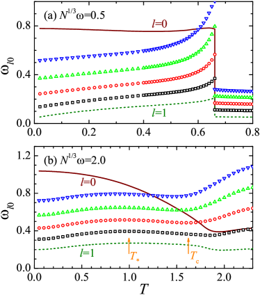
Figure 4: The mode frequencies $\omega_{l,n=0}$ of the breathing mode ($l=0$, solid lines), dipole mode ($l=1$, dotted lines) and surface modes ($l=2,3,4,5$, symbols from bottom to top) as a function of temperature $T$ at $N^{1/3}\omega=0.5$ (a) and $N^{1/3}\omega=2.0$ (b). In (b), the two arrows indicate the crossover temperature $T_{*}$ and the superfluid transition temperature $T_{c}$, respectively. We note that, the dipole mode frequency $\omega_{10}$ is not precisely the trapping frequency $\omega$, due to the mean-field interaction potential in the HFB-Popov theory Hutchinson1997 .

Observation of the first-order transition. — The predicted first-order BEC transition can be straightforwardly probed from the jump in the condensate fraction, or more readily from the discontinuity in the central condensate density, as we discuss in detail in Supplemental Material SM . For small effective trapping frequency, we find that the central condensate density is nearly unchanged below the superfluid transition and suddenly drops to zero right at the critical temperature $T_{c}$ SM .

Alternatively, we may probe the first-order transition by measuring the collective excitations of the system. For small trapping frequency, the quantum droplet features peculiar surface modes known as ripplons Petrov2015 ; Hu2020c ; Baillie2017 . We find that the ripplon mode frequency $\omega_{l\geq 2,n=0}$ diverges towards the first-order BEC transition at $T_{c}$, as shown in Fig. 4(a). In contrast, at large trapping frequency there seems to be local minimum in the ripplon mode frequencies near the second-order BEC transition, as can be seen from Fig. 4(b). The ripplon mode frequencies also show a characteristic local maximum at about the crossover temperature $T_{*}$, which might experimentally be used to locate the smooth crossover from a quantum droplet to a superfluid gas.

Spin-polarized tritium atoms. —In previous theoretical studies of the quantum droplet stabilized by three-body interactions, spin-polarized tritium condensate has been suggested to be a good candidate Blume2002 ; Beslic2009 . We have further explored this possibility by investigating the hypervolume $D$ of tritium atoms, inspired by the recent universality work by Mestrom et al. Mestrom2020 . In the absence of Feshbach resonances, the $s$-wave scattering length $a\simeq-11.92r_{\textrm{vdW}}$ and the trimer energy $E_{T}\simeq-3.50\times 10^{-3}E_{\textrm{vdW}}$, where $r_{\textrm{vdW}}$ and $E_{\textrm{vdW}}$ are the characteristic length and energy of the van-der-Waals potential of tritium atoms Blume2002 . The trimer energy differs slightly from the universal value $E_{T,\textrm{uni}}\simeq-4.45\times 10^{-3}E_{\textrm{vdW}}$ WangPhDThesis , suggesting that the universal formalism for the hypervolume $D$ given by Mestrom et al. Mestrom2020 could be used. As there is no decay dimer channel, so $D$ is purely real, without the annoying three-body loss Zwerger2019 . We can further apply Feshbach resonances to tune both $a$ and $D$ to realize a cloud of three-body weakly interacting tritium atoms. Cooling and trapping spin-polarized hydrogen and deuterium have recently been realized using Zeeman decelerator Hogan2008 ; Wiederkehr2010 . The same technique can be applied to tritium ClarkBSThesis .

Conclusions. — We have proposed that three-body interacting bosons may experience a first-order Bose-Einstein condensation in a weak harmonic trapping potential, in sharp contrast to the conventional smooth condensation transition observed so far. This first-order transition can be unambiguously probed from the sudden jump in the central density and the divergent ripplon mode frequency at the critical temperature. We have suggested that spin-polarized tritium atoms could be a promising candidate for observing the predicted first-order Bose-Einstein condensation transition.

Appendix A The HFB-Popov theory

We start with the model Hamiltonian for $N$ three-body interacting bosons of mass $M$ in 3D harmonic traps $V_{T}(\mathbf{r})\equiv M\omega^{2}r^{2}/2$,

$$\hat{H}=\int d\mathbf{r}\mathcal{H}(\mathbf{r}),$$ (6)

where the Hamiltonian density is,

$$\mathcal{H}=\hat{\psi}^{\dagger}\left[-\frac{\hbar^{2}\nabla^{2}}{2M}+V_{T}-\mu\right]\hat{\psi}+\frac{g}{2}\hat{\psi}^{\dagger 2}\hat{\psi}^{2}+\frac{G}{6}\hat{\psi}^{\dagger 3}\hat{\psi}^{3}.$$ (7)

Here, $\hat{\psi}(\mathbf{r})$ and $\hat{\psi}^{\dagger}(\mathbf{r})$ are respectively the annihilation and creation field operators of bosons, $\mu$ is the chemical potential, and the attractive two-body and repulsive three-body interaction strengths are given by,

$$g \equiv \frac{4\pi\hbar^{2}a}{M}<0,$$ (8)

$$G \equiv \frac{\hbar^{2}D}{M}>0,$$ (9)

respectively. To derive the HFB-Popov equations, we follow the procedure in the seminal work by Allan Griffin Griffin1996 and decompose the field operator $\hat{\psi}(\mathbf{r})$ into a condensate wave-function $\Phi(\mathbf{r})$ and a field operator $\tilde{\psi}(\mathbf{r})$ for noncondensate atoms, i.e., $\hat{\psi}(\mathbf{r},t)\equiv\Phi(\mathbf{r})+\tilde{\psi}(\mathbf{r},t)$ and its Hermitian form $\hat{\psi}^{\dagger}(\mathbf{r},t)\equiv\Phi^{*}(\mathbf{r})+\tilde{\psi}^{\dagger}(\mathbf{r},t)$.

In the exact Heisenberg equation of motion for $\hat{\psi}(\mathbf{r})$,

$$i\hbar\frac{\partial\hat{\psi}\left(\mathbf{r},t\right)}{\partial t}=\left[-\frac{\hbar^{2}\nabla^{2}}{2M}+V_{T}-\mu\right]\hat{\psi}\left(\mathbf{r},t\right)+g\hat{\psi}^{\dagger}\hat{\psi}\hat{\psi}\left(\mathbf{r},t\right)+\frac{G}{2}\hat{\psi}^{\dagger}\hat{\psi}^{\dagger}\hat{\psi}\hat{\psi}\hat{\psi}\left(\mathbf{r},t\right),$$ (10)

let us take the thermal average and obtain,

$$\left[-\frac{\hbar^{2}\nabla^{2}}{2M}+V_{T}-\mu\right]\Phi(\mathbf{r})+g\bigl{\langle}\hat{\psi}^{\dagger}\hat{\psi}\hat{\psi}\bigr{\rangle}+\frac{G}{2}\bigl{\langle}\hat{\psi}^{\dagger}\hat{\psi}^{\dagger}\hat{\psi}\hat{\psi}\hat{\psi}\bigr{\rangle}=0.$$ (11)

The last two terms in the above equation of motion can be treated in the self-consistent mean-field approximation Griffin1996 , namely ($\tilde{n}\equiv\bigl{\langle}\tilde{\psi}^{\dagger}\tilde{\psi}\bigr{\rangle}$ and $\tilde{m}\equiv\bigl{\langle}\tilde{\psi}\tilde{\psi}\bigr{\rangle}$),

$$\bigl{\langle}\hat{\psi}^{\dagger}\hat{\psi}\hat{\psi}\bigr{\rangle}=\Phi^{2}\Phi^{*}+\Phi^{*}\bigl{\langle}\tilde{\psi}\tilde{\psi}\bigr{\rangle}+2\Phi\bigl{\langle}\tilde{\psi}^{\dagger}\tilde{\psi}\bigr{\rangle}=\Phi^{2}\Phi^{*}+\Phi^{*}\tilde{m}+2\Phi\tilde{n}$$ (12)

and

$$\bigl{\langle}\hat{\psi}^{\dagger}\hat{\psi}^{\dagger}\hat{\psi}\hat{\psi}\hat{\psi}\bigr{\rangle} = \Phi^{3}\Phi^{*2}+3\Phi\Phi^{*2}\bigl{\langle}\tilde{\psi}\tilde{\psi}\bigr{\rangle}+6\Phi^{2}\Phi^{*}\bigl{\langle}\tilde{\psi}^{\dagger}\tilde{\psi}\bigr{\rangle}+\Phi^{3}\bigl{\langle}\tilde{\psi}^{\dagger}\tilde{\psi}^{\dagger}\bigr{\rangle}+2\Phi^{*}\bigl{\langle}\tilde{\psi}^{\dagger}\tilde{\psi}\tilde{\psi}\tilde{\psi}\bigr{\rangle}+3\Phi\bigl{\langle}\tilde{\psi}^{\dagger}\tilde{\psi}^{\dagger}\tilde{\psi}\tilde{\psi}\bigr{\rangle},$$ (13)

$$= \Phi^{3}\Phi^{*2}+3\Phi\Phi^{*2}\tilde{m}+6\Phi^{2}\Phi^{*}\tilde{n}+\Phi^{3}\tilde{m}^{*}+6\Phi^{*}\tilde{n}\tilde{m}+3\Phi\left(2\tilde{n}^{2}+\tilde{m}\tilde{m}^{*}\right).$$

Here, we have decoupled the four-field-operator terms according to the Wick theorem,

$$\bigl{\langle}\tilde{\psi}^{\dagger}\tilde{\psi}\tilde{\psi}\tilde{\psi}\bigr{\rangle} = 3\tilde{n}\tilde{m},$$ (14)

$$\bigl{\langle}\tilde{\psi}^{\dagger}\tilde{\psi}^{\dagger}\tilde{\psi}\tilde{\psi}\bigr{\rangle} = 2\tilde{n}^{2}+\tilde{m}\tilde{m}^{*}.$$ (15)

Therefore, we find the time-independent generalized Gross-Pitaevskii (GP) equation ($n_{c}\equiv\left|\Phi(\mathbf{r})\right|^{2}$),

$${\color[rgb]{0,0,0}\left[-\frac{\hbar^{2}\nabla^{2}}{2M}+V_{T}-\mu\right]\Phi+g\left(n_{c}+2\tilde{n}\right)\Phi+{\normalcolor{\color[rgb]{1,0,0}g\tilde{m}\Phi^{*}}}+\frac{G}{2}\left(n_{c}^{2}+6n_{c}\tilde{n}+6\tilde{n}^{2}+{\color[rgb]{1,0,0}\Phi^{2}\tilde{m}^{*}+3\tilde{m}\tilde{m}^{*}}\right)\Phi+{\color[rgb]{1,0,0}\frac{3G}{2}\left(n_{c}\tilde{m}+2\tilde{n}\tilde{m}\right)\Phi^{*}}=0.}$$ (16)

It is well-known that a nonzero anomalous correlation $\tilde{m}\equiv\bigl{\langle}\tilde{\psi}\tilde{\psi}\bigr{\rangle}$ gives rise to a gapped excitation spectrum Griffin1996 ; Shi1998 , even in the absence of the three-body interacting term, which is unphysical. Therefore, we take the Popov approximation $\tilde{m}=0$ and $\tilde{m}^{*}=0$ everywhere in the generalized GP equation. This leads to the form,

$$\mathcal{\hat{L}}\Phi\left(\mathbf{r}\right)\equiv\left[-\frac{\hbar^{2}\nabla^{2}}{2M}+V_{T}+g\left(n_{c}+2\tilde{n}\right)+G\left(\frac{n_{c}^{2}}{2}+3n_{c}\tilde{n}+3\tilde{n}^{2}\right)\right]\Phi\left(\mathbf{r}\right)=\mu\Phi\mathbf{\left(r\right)}.$$ (17)

The generalized Hartree-Fock-Bogoliubov equation for quasi-particles may be derived from the equation of motion for the field operator $\tilde{\psi}(\mathbf{r})$ of noncondensate atoms Griffin1996 , which can be obtained by subtracting Eq. (11) from Eq. (10). It can also be equivalently derived by expanding the model Hamiltonian to the quadratic terms of $\tilde{\psi}^{\dagger}$ and $\tilde{\psi}$ Griffin1996 . This alternative derivation is useful to determine the expressions of the thermodynamic potential and free energy. Therefore, let us describe it in detail. We first consider the two-body interaction term,

$$\hat{\psi}^{\dagger 2}\hat{\psi}^{2} = \Phi^{2}\Phi^{*2}+\Phi^{2}\tilde{\psi}^{\dagger}\tilde{\psi}^{\dagger}+4\Phi\Phi^{*}\tilde{\psi}^{\dagger}\tilde{\psi}+\Phi^{*2}\tilde{\psi}\tilde{\psi}+\tilde{\psi}^{\dagger}\tilde{\psi}^{\dagger}\tilde{\psi}\tilde{\psi},$$ (18)

$$= \left[\left(\Phi^{2}+\tilde{m}\right)\tilde{\psi}^{\dagger}\tilde{\psi}^{\dagger}+\textrm{h.c.}\right]+4\left(n_{c}+\tilde{n}\right)\tilde{\psi}^{\dagger}\tilde{\psi}+n_{c}^{2}-\left(2\tilde{n}^{2}+\tilde{m}\tilde{m}^{*}\right).$$

In the second line of the above equation, we have taken the self-consistent mean-field approximation to $\tilde{\psi}^{\dagger}\tilde{\psi}^{\dagger}\tilde{\psi}\tilde{\psi}$, i.e.,

$$\tilde{\psi}^{\dagger}\tilde{\psi}^{\dagger}\tilde{\psi}\tilde{\psi}=\tilde{m}\tilde{\psi}^{\dagger}\tilde{\psi}^{\dagger}+4\tilde{n}\tilde{\psi}^{\dagger}\tilde{\psi}+\tilde{m}^{*}\tilde{\psi}\tilde{\psi}-\left(2\tilde{n}^{2}+\tilde{m}\tilde{m}^{*}\right).$$ (19)

The three-body interaction term can be treated in a similar way. We find that,

$$\hat{\psi}^{\dagger 3}\hat{\psi}^{3}=n_{c}^{3}+\left(3\Phi^{3}\Phi^{*}\tilde{\psi}^{\dagger}\tilde{\psi}^{\dagger}+\textrm{h.c.}\right)+9n_{c}^{2}\tilde{\psi}^{\dagger}\tilde{\psi}+9n_{c}\tilde{\psi}^{\dagger}\tilde{\psi}^{\dagger}\tilde{\psi}\tilde{\psi}+\left(3\Phi^{2}\tilde{\psi}^{\dagger}\tilde{\psi}^{\dagger}\tilde{\psi}^{\dagger}\tilde{\psi}+\textrm{h.c.}\right)+\tilde{\psi}^{\dagger 3}\tilde{\psi}^{3}.$$ (20)

By inserting the mean-field decoupling, i.e.,

$$\tilde{\psi}^{\dagger}\tilde{\psi}^{\dagger}\tilde{\psi}^{\dagger}\tilde{\psi} = 3\tilde{n}\tilde{\psi}^{\dagger}\tilde{\psi}^{\dagger}+3\tilde{m}^{*}\tilde{\psi}^{\dagger}\tilde{\psi}-3\tilde{n}\tilde{m}^{*},$$ (21)

$$\tilde{\psi}^{\dagger 3}\tilde{\psi}^{3} = 9\left[\tilde{n}\tilde{m}\tilde{\psi}^{\dagger}\tilde{\psi}^{\dagger}+\left(2\tilde{n}^{2}+\tilde{m}\tilde{m}^{*}\right)\tilde{\psi}^{\dagger}\tilde{\psi}+\tilde{n}\tilde{m}^{*}\tilde{\psi}\tilde{\psi}\right]-\left(12\tilde{n}^{3}+18\tilde{n}\tilde{m}\tilde{m}^{*}\right),$$ (22)

we obtain that,

$$\hat{\psi}^{\dagger 3}\hat{\psi}^{3} = \left[\left(3\Phi^{3}\Phi^{*}+9n_{c}\tilde{m}+9\Phi^{2}\tilde{n}+9\tilde{n}\tilde{m}\right)\tilde{\psi}^{\dagger}\tilde{\psi}^{\dagger}+\textrm{h.c.}\right]+9\left(n_{c}^{2}+\Phi^{2}\tilde{m}^{*}+\Phi^{*2}\tilde{m}+4n_{c}\tilde{n}+2\tilde{n}^{2}+\tilde{m}\tilde{m}^{*}\right)\tilde{\psi}^{\dagger}\tilde{\psi}$$ (23)

$$+n_{c}^{3}-\left[\left(9\Phi^{2}\tilde{n}\tilde{m}^{*}+\textrm{h.c.}\right)+9n_{c}\left(2\tilde{n}^{2}+\tilde{m}\tilde{m}^{*}\right)+12\tilde{n}^{3}+18\tilde{n}\tilde{m}\tilde{m}^{*}\right].$$

By collecting all the bilinear terms in the field operators, we may rewrite the the Hamiltonian density within the Hartree-Fock-Bogoliubov approximation as,

$$\mathcal{H}_{\textrm{HFB}}=\frac{1}{2}\left[\begin{array}[]{cc}\tilde{\psi}^{\dagger},&\tilde{\psi}\end{array}\right]\left[\begin{array}[]{cc}\mathcal{\hat{K}}_{\textrm{HFB}}-\mu&\mathcal{\hat{M}}_{\textrm{HFB}}\\ \mathcal{\hat{M}}_{\textrm{HFB}}&\hat{\mathcal{K}}_{\textrm{HFB}}-\mu\end{array}\right]\left[\begin{array}[]{c}\tilde{\psi}\\ \tilde{\psi}^{\dagger}\end{array}\right]+\Omega_{\textrm{HFB}}^{(0)}\left(\mathbf{r}\right),$$ (24)

where we have defined the operators

$$\mathcal{\hat{K}}_{\textrm{HFB}} \equiv -\frac{\hbar^{2}\nabla^{2}}{2M}+V_{T}+2g\left(n_{c}+\tilde{n}\right)+\frac{3}{2}G\left(n_{c}^{2}+{\color[rgb]{1,0,0}\Phi^{2}\tilde{m}^{*}}+{\color[rgb]{0,.5,.5}{\color[rgb]{1,0,0}\Phi^{*2}\tilde{m}}}+4n_{c}\tilde{n}+2\tilde{n}^{2}+{\color[rgb]{1,0,0}\tilde{m}\tilde{m}^{*}}\right),$$ (25)

$$\mathcal{\hat{M}}_{\textrm{HFB}} \equiv g\left(\Phi^{2}+{\color[rgb]{1,0,0}\tilde{m}}\right)+G\left(n_{c}\Phi^{2}+{\color[rgb]{1,0,0}3n_{c}\tilde{m}}+3\Phi^{2}\tilde{n}+{\color[rgb]{1,0,0}3n\tilde{m}}\right),$$ (26)

and

$$\Omega_{\textrm{HFB}}^{(0)}\left(\mathbf{r}\right) \equiv \Phi^{*}\left[-\frac{\hbar^{2}\nabla^{2}}{2M}+V_{T}-\mu\right]\Phi+\frac{g}{2}\left(n_{c}^{2}-2\tilde{n}^{2}-{\color[rgb]{1,0,0}\tilde{m}\tilde{m}^{*}}\right)$$ (27)

$$+\frac{G}{6}\left[n_{c}^{3}-\left({\color[rgb]{1,0,0}9\Phi^{2}\tilde{n}\tilde{m}^{*}+\textrm{h.c.}}\right)-9n_{c}\left(2\tilde{n}^{2}+{\color[rgb]{1,0,0}\tilde{m}\tilde{m}^{*}}\right)-12\tilde{n}^{3}-{\color[rgb]{1,0,0}18\tilde{n}\tilde{m}\tilde{m}^{*}}\right]$$

is the density of the mean-field thermodynamic potential at zero temperature. Let us now take the Popov approximation and set $\tilde{m}=0$ and $\tilde{m}^{*}=0$ in $\mathcal{\hat{K}}_{\textrm{HFB}}$, $\mathcal{\hat{M}}_{\textrm{HFB}}$ and $\Omega_{\textrm{HFB}}^{(0)}(\mathbf{r})$. By further assuming a real ground-state condensate wave-function $\Phi(\mathbf{r})$, it is easy to see that $\mathcal{\hat{M}}_{\textrm{HFB}}$ becomes

$$\hat{\mathcal{M}}=gn_{c}+G\left(n_{c}^{2}+3n_{c}\tilde{n}\right),$$ (28)

and $\mathcal{\hat{K}}_{\textrm{HFB}}$ can be rewrite as,

$$\hat{\mathcal{K}}=\mathcal{\hat{L}}+\mathcal{\hat{M}},$$ (29)

where the operator $\mathcal{\hat{L}}$ is defined in Eq. (17). Also, $\Omega_{\textrm{HFB}}^{(0)}(\mathbf{r})$ takes the form,

$$\Omega^{(0)}\left(\mathbf{r}\right)=\Phi^{*}\left[-\frac{\hbar^{2}\nabla^{2}}{2M}+V_{T}-\mu\right]\Phi+g\left(\frac{n_{c}^{2}}{2}-\tilde{n}^{2}\right)+G\left(\frac{n_{c}^{3}}{6}-3n_{c}\tilde{n}^{2}-2\tilde{n}^{3}\right).$$ (30)

From the Hamiltonian density for the field operators of non-condensate atoms, Eq. (24), we directly write down the coupled HFB-Popov equations for the $\eta$-th quasi-particle wave-functions $u_{\eta}$ and $v_{\eta}$ with energy $E_{\eta}>0$,

$$\left[\begin{array}[]{cc}\hat{\mathcal{L}}-\mu+\mathcal{\hat{M}}&\mathcal{\hat{M}}\\ \mathcal{\hat{M}}&\hat{\mathcal{L}}-\mu+\mathcal{\hat{M}}\end{array}\right]\left[\begin{array}[]{c}u_{\eta}\left(\mathbf{r}\right)\\ v_{\eta}\left(\mathbf{r}\right)\end{array}\right]=E_{\eta}\left[\begin{array}[]{c}+u_{\eta}\left(\mathbf{r}\right)\\ -v_{\eta}\left(\mathbf{r}\right)\end{array}\right].$$ (31)

The total thermodynamic potential at finite temperature $T$ is given by,

$$\Omega={\color[rgb]{0,0,1}\Omega_{\textrm{LHY}}^{(0)}}+k_{B}T\sum_{\eta}\ln\left[1-e^{-\beta E_{\eta}}\right]+\int d\mathbf{r}\Omega^{(0)}\left(\mathbf{r}\right),$$ (32)

where $\beta=1/(k_{B}T)$ is the inverse temperature and

$$\Omega_{\textrm{LHY}}^{(0)}\equiv-\sum_{\eta}\int d\mathbf{r}E_{\eta}\left|v_{\eta}\mathbf{\left(r\right)}\right|^{2}$$ (33)

is the contribution of quantum fluctuations to the thermodynamic potential, the so-called Lee-Huang-Yang (LHY) energy term Dalfovo1999 . Once the quasi-particle wave-functions are obtained, the noncondensate density can be calculated according to,

$$\tilde{n}\left(\mathbf{r}\right)={\color[rgb]{0,0,1}\tilde{n}_{\textrm{qd}}\left(\mathbf{r}\right)}+\sum_{\eta}\frac{\left|u_{\eta}\left(\mathbf{r}\right)\right|^{2}+\left|v_{\eta}\mathbf{\left(r\right)}\right|^{2}}{e^{\beta E_{\eta}}-1},$$ (34)

where $\tilde{n}_{\textrm{qd}}(\mathbf{r})=\sum_{\eta}\left|v_{\eta}\mathbf{(r})\right|^{2}$ is the depletion to the condensate arising from quantum fluctuations and is the only contribution to density at zero temperature.

Eq. (17) and Eq. (31), together with Eq. (34) and $n_{c}=\left|\Phi(\mathbf{r})\right|^{2}$, form a closed set of HFB-Popov equations that should be solved self-consistently Hutchinson1997 . The chemical potential $\mu$ should be adjusted to satisfy the number equation $N=\int d\mathbf{r}[n_{c}(\mathbf{r})+\tilde{n}(\mathbf{r})]\equiv N_{c}+N_{\textrm{th}}$.

The HFB-Popov theory has been extensively used to describe weakly interacting Bose gases at finite temperature Hutchinson1997 . The advantages and shortages of such a theory are now well understood. In particular, it is known that the theory does not provide accurate descriptions at both zero temperature and at temperatures sufficiently close to the superfluid transition Shi1998 . At zero temperature, this is because the anomalous correlation $\tilde{m}(\mathbf{r})$ neglected in the Popov approximation becomes comparable to the normal correlation, i.e., $\tilde{n}_{\textrm{qd}}(\mathbf{r})$, if we critically examine the role of zero-temperature quantum fluctuations. For the consistency of the theory, thus it seems necessary to discard the quantum depletion $\tilde{n}_{\textrm{qd}}\left(\mathbf{r}\right)$ and the LHY energy term $\Omega_{\textrm{LHY}}^{(0)}$. This treatment is well justified for a weakly interacting Bose gas with a repulsive two-body interaction alone, where the quantum depletion (or the LHY energy) contributes only a few percent to the total density (or the total energy) Hutchinson1997 . For a three-body interacting quantum droplet considered in this work, as we shall discuss below, we find that the quantum depletion is typically at about 10%, much smaller than that of a superfluid helium droplet, where 90% of atoms are out of the condensate at $T=0$. In the vicinity of the superfluid transition $T_{c}$, it is also known that the Popov approximation predicts a spurious first-order superfluid transition for a homogeneous Bose gas, as characterized by a very small jump (i.e., about a few percent) in the condensate density Shi1998 . This spurious feature is not important and does not show up when the system is confined in a harmonic trap.

Appendix B Numerical calculations

At zero temperature, where the noncondensate density $\tilde{n}=0$ as we neglect the quantum depletion, the generalized GP equation Eq. (17) in free space (i.e., $V_{T}=0$) takes the form,

$$\left[-\frac{\hbar^{2}\nabla^{2}}{2M}+g\left|\Phi\right|^{2}+\frac{G}{2}\left|\Phi\right|^{4}\right]\Phi=\mu\Phi.$$ (35)

As $g<0$ and $G>0$, this GP equation admits a self-bound droplet as the ground state for sufficiently large number of atoms $N=\int d\mathbf{r}\left|\Phi\right|^{2}\gg 1$. To see this, let us check the case of an infinitely large number of atoms, where we can safely neglect the surface effect and remove the first kinetic term (i.e., the $\nabla^{2}$ term). We find that the bulk chemical potential ($n=\left|\Phi\right|^{2}$),

$$\mu\left(n\right)=gn+\frac{G}{2}n^{2},$$ (36)

and consequently the energy per particle,

$$\frac{\epsilon\left(n\right)}{n}=\frac{g}{2}n+\frac{G}{6}n^{2}.$$ (37)

It is clear that the energy per particle acquires a minimum at the equilibrium density,

$$n_{0}=\frac{3}{2}\frac{\left(-g\right)}{G}=6\pi\frac{\left|a\right|}{D},$$ (38)

at which the pressure $P$ vanishes due to the thermodynamic relation,

$$P=\left[n^{2}\frac{\partial\left(\epsilon/n\right)}{\partial n}\right]_{n=n_{0}}=0.$$ (39)

The system is therefore self-bound into a droplet state at zero pressure, in equilibrium with the surrounding vacuum. In the absence of the external harmonic trap, the center density would be fixed to $n_{0}$, if we neglect the boundary (surface) effect. When we add the particles to the droplet, the droplet expands and increases its radius, while keeping its bulk density unchanged.

B.1 Re-scaled units

In numerical calculations, it is convenient to introduce the units for length, density and also energy, and to make the equations dimensionless. For the density unit, the equilibrium density $n_{0}$ is a natural choice. To fix the length unit $\xi$, let us require that the three-body term in the energy per particle assumes the following simple form,

$$\frac{G}{6}n^{2}\rightarrow\frac{\bar{G}}{6}\bar{n}^{2}=\bar{n}^{2},$$ (40)

after we use the re-scaled units (as indicated by the bar above the variables). This means that the dimensionless three-body interaction strength is,

$$\bar{G}\equiv\frac{Gn_{0}^{2}}{\hbar^{2}/\left(M\xi^{2}\right)}=+6,$$ (41)

where $\hbar^{2}/(M\xi^{2})$ is the energy unit related to the length unit $\xi$. By substituting $G=\hbar^{2}D/M$ and the equilibrium density $n_{0}$, we find that,

$$\xi=\sqrt{\frac{D}{6\pi^{2}a^{2}}}.$$ (42)

It is straightforward to check that the two-body interaction strength then becomes,

$$\bar{g}\equiv\frac{gn_{0}}{\hbar^{2}/\left(M\xi^{2}\right)}=-4.$$ (43)

From now on, we will use the re-scaled units for length $\mathbf{\bar{r}}\equiv\mathbf{r}/\xi$, density $\bar{n}\equiv n/n_{0}$, energy $\bar{E}_{\eta}\equiv M\xi^{2}E_{\eta}/\hbar^{2}$ and trapping frequency $\bar{\omega}=M\xi^{2}\omega/\hbar$. The re-scaled condensate wave-function is $\bar{\Phi}=\Phi/\sqrt{n_{0}}$. The reduced number of particles is given by $\bar{N}=N/(n_{0}\xi^{3})$ with

$$n_{0}\xi^{3}=\frac{\sqrt{D/6}}{\pi^{2}a^{2}}.$$ (44)

and the number equation becomes,

$$\bar{N}=\int d\mathbf{\bar{r}}\frac{n_{c}\left(\mathbf{\bar{r}}\right)+\tilde{n}\left(\mathbf{\bar{r}}\right)}{n_{0}}\equiv\bar{N}_{c}+\bar{N}_{\textrm{th}}.$$ (45)

Hereafter, for convenience we shall remove the bar for all the re-scaled units.

In the dimensionless form ($g=-4$ and $G=+6$, and effectively $\hbar=M=1$), the zero-temperature GP equation Eq. (35) then becomes very simple,

$$\left[-\frac{\nabla^{2}}{2}+\frac{\omega^{2}r^{2}}{2}-4\Phi^{2}+3\Phi^{4}\right]\Phi=\mu\Phi,$$ (46)

where we have re-inserted the harmonic trap term. We see that this equation depends on two controlling variables, the dimensionless trapping frequency $\omega$ and the reduced number of particle $N$, both of which involves the microscopic parameters of the model Hamiltonian such as the two-body scattering length $a$ and the three-body scattering hypervolume $D$. Eq. (46) has been discussed in detail in the previous work Hu2020c . It turns out that for a large reduced number of particles, we can neglect the finite-size effect and the properties of the system actually depend on a single parameter $N^{1/3}\omega$. In our calculations, we typically take the reduced number of particles $N=1000$.

B.2 Technical difficulties

The dimensionless HPB-Popov equations with the operators $\hat{\mathcal{L}}$ and $\hat{\mathcal{M}}$, obtained by setting $\hbar=M=1$, $g=-4$ and $G=+6$, can be solved by the routines outlined in the previous work Hutchinson1997 ; Hu2020c ; Wang2020b . The following three challenges in the numerical calculations are worth noting.

First, for a droplet state, there are numerous quasiparticle energy levels accumulated just above the particle emission threshold $\left|\mu\right|$ Hu2020c . The energy level separation is set by the harmonic trapping frequency $\omega$. To solve this difficulty, we consider a dimensionless trapping frequency $\omega\geq 0.03$ and typically use several-hundred expansion basis functions in solving the quasi-particle wave-functions $u_{\eta}$ and $v_{\eta}$ for a given angular momentum $l$ (which is a good quantum number for our spherical harmonic traps). Further improvement on the numerical accuracy could be achieved by considering the 5-th order $B$-spline basis Wang2020b . The $B$-spline basis would allow us to use an uneven grid, which might better represent the solution wave-function. It also allows a higher order approximation of the derivative operator that appears in the kinetic energy term.

On the other hand, at finite temperature $T\neq 0$ we must iterate the solutions of the GP equation Eq. (17) for the condensate wave-function and the HFB-Popov equations Eq. (31) for the quasi-particle wave-functions, in order to gradually improve the thermal density $\tilde{n}(\mathbf{r})$ for convergence. This iterative procedure turns out to be very slow with increasing temperature. In particular, sufficiently close to the superfluid transition, the small number of condensed particles $N_{c}\sim O(1)$ implies that the chemical potential $\mu$ appearing in the GP equation (i.e., the lowest eigenvalue of the operator $\mathcal{\hat{L}}$ in the zero momentum $l=0$ sector) can no longer be treated as the chemical potential of the whole system. To solve this problem, we introduce a new chemical potential $\mu_{t}$ of the whole system, by requiring that,

$$\frac{1}{e^{\left(\mu-\mu_{t}\right)/k_{B}T}-1}=N_{c}.$$ (47)

The difference between the two chemical potentials

$$\mu-\mu_{t}=k_{B}T\ln\left(1+\frac{1}{N_{c}}\right)\sim\frac{k_{B}T}{N_{c}}$$ (48)

is negligibly small away from the superfluid transition when $N_{c}\gg 1$. However, in the vicinity of the superfluid transition, in the Bose-Einstein distribution function $f_{B}(E_{\eta}$) we have to measure the energy $E_{\eta}$ of the Bogoliubov quasiparticles with respect to $\mu_{t}$, instead of $\mu$. This leads to a modified expression for the thermal density (in the case of excluding the quantum depletion),

$$\tilde{n}\left(\mathbf{r}\right) = \sum_{\eta}\frac{\left|u_{\eta}\left(\mathbf{r}\right)\right|^{2}+\left|v_{\eta}\mathbf{\left(r\right)}\right|^{2}}{e^{\beta\left(E_{\eta}+\mu-\mu_{t}\right)}-1}$$ (49)

$$= \sum_{\eta}\frac{\left|u_{\eta}\left(\mathbf{r}\right)\right|^{2}+\left|v_{\eta}\mathbf{\left(r\right)}\right|^{2}}{\left(1+1/N_{c}\right)e^{\beta E_{\eta}}-1}.$$

The thermal contribution to the thermodynamic potential in Eq. (32) is modified in a similar way (i.e., by replacing $E_{\eta}$ with $E_{\eta}+\mu-\mu_{t}$).

Finally, a large temperature leads to the significant population of the high-energy quasi-particle energy levels, which would require a large number of the expansion basis functions in solving the HFB-Popov equations and therefore considerably slow down our numerical calculations. To avoid this problem, we consider the use of the local-density approximation (LDA) for the high-lying quasi-particle wave-functions Liu2007 . For this purpose, we introduce a high-energy cut-off $E_{c}$. For the quasi-particle energy $E_{\eta}>E_{c}$, we treat the quasi-particle wave-functions locally (at the position $r$) as plane-waves with amplitudes $u_{\mathbf{k}}(r)$ and $v_{\mathbf{k}}(r)$ at the momentum $\mathbf{k}$ Liu2007 . The HFB-Popov equations for the quasi-particles then become,

$$\left[\begin{array}[]{cc}\frac{k^{2}}{2}+\mathcal{V}_{\textrm{eff}}(r)&\mathcal{M}(r)\\ \mathcal{M}(r)&\frac{k^{2}}{2}+\mathcal{V}_{\textrm{eff}}(r)\end{array}\right]\left[\begin{array}[]{c}u_{\mathbf{k}}\\ v_{\mathbf{k}}\end{array}\right]=E_{\mathbf{k}}\left[\begin{array}[]{c}+u_{\mathbf{k}}\\ -v_{\mathbf{k}}\end{array}\right],$$ (50)

where

$$\mathcal{V}_{\textrm{eff}} = \frac{\omega^{2}r^{2}}{2}-\mu-8\left(n_{c}+\tilde{n}\right)+9n_{c}^{2}+36n_{c}\tilde{n}+6\tilde{n}^{2},$$ (51)

$$\mathcal{M} = -4n_{c}+6n_{c}^{2}+18n_{c}\tilde{n},$$ (52)

from which we obtain,

$$u_{\mathbf{k}}^{2}(r) = \frac{1}{2}\left[\frac{k^{2}/2+\mathcal{V}_{\textrm{eff}}\left(r\right)}{E_{\mathbf{k}}\left(r\right)}+1\right],$$ (53)

$$v_{\mathbf{k}}^{2}(r) = \frac{1}{2}\left[\frac{k^{2}/2+\mathcal{V}_{\textrm{eff}}\left(r\right)}{E_{\mathbf{k}}\left(r\right)}-1\right],$$ (54)

and

$$E_{\mathbf{k}}(r)=\sqrt{\left[k^{2}/2+\mathcal{V}_{\textrm{eff}}(r)\right]^{2}-\mathcal{M}^{2}(r)}.$$ (55)

At the position $r$, therefore the LDA contribution from the continuous high-lying energy levels to the thermal density (i.e., $E_{\mathbf{k}}(r)>E_{c}$) is,

$$\tilde{n}_{H}\left(\mathbf{r}\right)=\int\frac{d\mathbf{k}}{\left(2\pi\right)^{3}}\frac{\left[\frac{k^{2}}{2}+\mathcal{V}_{\textrm{eff}}(r)\right]/E_{\mathbf{k}}(r)}{\left(1+1/N_{c}\right)e^{\beta E_{\mathbf{k}}(r)}-1}.$$ (56)

Together with the contribution from the discrete low-lying energy levels,

$$\tilde{n}_{L}\left(\mathbf{r}\right)=\sum_{E_{\eta}<E_{c}}\frac{\left|u_{\eta}\left(\mathbf{r}\right)\right|^{2}+\left|v_{\eta}\mathbf{\left(r\right)}\right|^{2}}{\left(1+1/N_{c}\right)e^{\beta E_{\eta}}-1},$$ (57)

we obtain the total thermal density,

$$\tilde{n}(\mathbf{r})=\tilde{n}_{L}\left(\mathbf{r}\right)+\tilde{n}_{H}\left(\mathbf{r}\right).$$ (58)

The LDA treatment for the high-lying quasi-particle energy levels turns out to be very efficient. Our numerical results are essentially independent on the cut-off energy $E_{c}$, provided that it is reasonably large.

Appendix C Quantum depletion

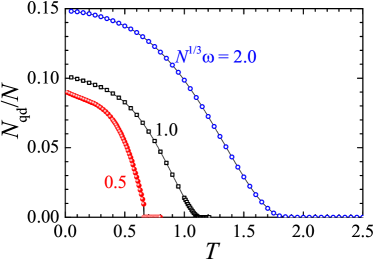
Figure 5: Quantum depletion $N_{\textrm{qd}}/N$ as a function of temperature at three effective trapping frequencies $N^{1/3}\omega=0.5$, $1.0$ and $2.0$. The depletion is typically about $10\%$. It vanishes when we increase the temperature towards the superfluid transition.

We have self-consistently (and iteratively) solved the coupled HFB-Popov equations, without the inclusion of the quantum depletion $\tilde{n}_{\textrm{qd}}(\mathbf{r})$ in the thermal density $\tilde{n}(\mathbf{r})$. We have then calculated the number of quantum depleted atoms $N_{\textrm{qd}}=\int d\mathbf{r}\sum_{\eta}\left|v_{\eta}\mathbf{(r})\right|^{2}$ for a self-consistent check. The results are shown in Fig. 5, where we consider the temperature dependence of the ratio $N_{\textrm{qd}}/N$ at three effective trapping frequencies. We have also tried the inclusion of $\tilde{n}_{\textrm{qd}}(\mathbf{r})$ in the thermal density $\tilde{n}(\mathbf{r})$ in our numerical iterations and have found qualitatively similar predictions.

It is readily seen that the quantum depletion is typically at around $10\%$ at zero temperature. Actually, we would anticipate that the zero-temperature quantum depletion should be a universal constant in the absence of the external harmonic trap (i.e., about $8\%$), where the bulk density of the droplet state is precisely the equilibrium density $n_{0}$. The increase of the zero-temperature quantum depletion with increasing effective trapping frequency should be contributed to the enhanced central density due to the external trapping potential.

At nonzero temperature, the quantum depletion decreases as anticipated. It becomes negligibly small close to the superfluid transition. As in this work we are mostly interested in the region near the superfluid transition, the consistent exclusion of the quantum depletion in our HFB-Popov calculations therefore seems well justified.

Appendix D First-order BEC transition temperature

The first-order BEC transition temperature at small effective trapping frequency $N^{1/3}\omega\rightarrow 0$ might be analytically derived. To see this, let us consider the free energy $F_{S}(T)$ of the superfluid quantum droplet state and the free energy $F_{N}(T)$ of a normal Bose gas.

D.1 The normal-state free energy $F_{N}(T)$

For the normal phase, since the trapping frequency is very small, the atomic cloud is dilute and can be treated as a non-interacting Bose gas. The free energy can then be obtained in the semi-classical approximation Dalfovo1999 ,

$$F_{N}=\iint\frac{d\mathbf{k}d\mathbf{r}}{\left(2\pi\right)^{3}}\ln\left[1-e^{-\beta\left(\frac{\hbar^{2}k^{2}}{2m}+V_{T}-\mu\right)}\right]+\mu N,$$ (59)

where the chemical potential $\mu$ satisfies,

$$N=\iint\frac{d\mathbf{k}d\mathbf{r}}{\left(2\pi\right)^{3}}\frac{1}{e^{\beta\left(\frac{\hbar^{2}k^{2}}{2m}+V_{T}-\mu\right)}-1}.$$ (60)

These Bose-type integrals can be worked out explicitly, with the help of the polylogarithm function $\textrm{Li}_{\nu}(z)$, i.e.,

$$\int_{0}^{\infty}d\epsilon\frac{\epsilon^{\nu-1}}{e^{\beta\left(\epsilon-\mu\right)-1}}=\left(k_{B}T\right)^{\nu}\Gamma\left(\nu\right)\textrm{Li}_{\nu}\left(z\right),$$ (61)

where the fugacity $z\equiv e^{\beta\mu}$ and $\Gamma(\nu)$ is the Gamma function. We find that Dalfovo1999 ,

$$\frac{F_{N}}{N} = k_{B}T\frac{\textrm{Li}_{4}\left(z\right)}{\textrm{Li}_{3}\left(z\right)}+\mu,$$ (62)

$$N = \left(\frac{k_{B}T}{\hbar\omega}\right)^{3}\textrm{Li}_{3}\left(z\right).$$ (63)

In the normal phase, the fugacity $z$ turns out to be very small. Indeed, below the condensation transition the chemical potential $\mu$ must turn into the bulk chemical potential of the droplet state, i.e., $\mu_{0}=gn_{0}+Gn_{0}^{2}/2<0$, which serves as the energy unit after we re-scale and make the equations dimensionless. For example, by taking $g=-4$, $G=+6$ and $n_{0}=1$, we obtain $\mu_{0}=-1$. Therefore, it is reasonable to Taylor expand the expressions of the free energy and the number of particles, in terms of the small fugacity $z\sim e^{\mu_{0}/(k_{B}T)}\ll 1$ at low temperature $k_{B}T\ll\left|\mu_{0}\right|$. In the re-scaled units, after we take $k_{B}=1$ and $\hbar=1$, we then obtain that,

$$\frac{F_{N}}{N\left|\mu_{0}\right|} \simeq T\left(1-\frac{z}{16}\right)+T\ln z,$$ (64)

$$N\omega^{3} \simeq T^{3}z\left(1+\frac{z}{8}\right).$$ (65)

By re-expressing the fugacity $z$ in terms of the temperature $T$, to the leading order we finally arrive at,

$$\frac{F_{N}}{N\left|\mu_{0}\right|}\simeq 3T\ln\frac{N^{1/3}\omega}{T}.$$ (66)

D.2 The droplet-state free energy $F_{S}(T)$

At low temperature, the free energy $F_{S}(T)$ is essentially the zero-temperature total energy $E(T=0)$ of the droplet, if we neglect the small surface effect for a large droplet (with $N\gg 1$). By using Eq. (37), in the re-scaled units we find that,

$$\frac{F_{S}}{N\left|\mu_{0}\right|}\simeq-1.$$ (67)

This expression is easy to understand. At zero temperature we anticipate that all the atoms are bounded into the droplet with the binding energy $\left|\mu_{0}\right|$.

D.3 First-order superfluid transition temperature

Using the condition $F_{N}(T)=F_{S}(T)$ at the transition temperature $T_{c}$, we obtain

$$3T_{c}\ln\frac{N^{1/3}\omega}{T_{c}}=-1,$$ (68)

or

$$N^{1/3}\omega=T_{c}\exp\left(-\frac{1}{3T_{c}}\right).$$ (69)

By restoring the full units, we find that,

$$N^{1/3}\hbar\omega=k_{B}T_{c}\exp\left(\frac{\mu_{0}}{3k_{B}T_{c}}\right),$$ (70)

where the bulk chemical potential takes the form,

$$\mu_{0}=-\frac{3g^{2}}{8G}.$$ (71)

It is clear that the critical temperature eventually goes to zero, $T_{c}\rightarrow 0$, when we gradually remove the external harmonic trapping potential, $\omega\rightarrow 0$.

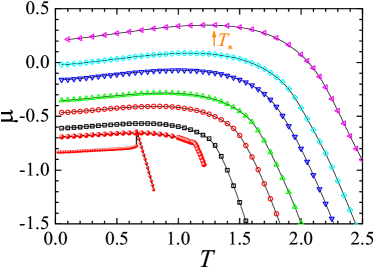
Figure 6: Temperature dependence of the chemical potential at different effective trapping frequency $N^{1/3}\omega$. From bottom to top, the value of $N^{1/3}\omega$ is $0.5$, $1.0$, $1.2$, $1.5$, $1.7$, $2.0$, $2.2$, and $2.5$.

Appendix E The characteristic temperature $T_{*}$ from the chemical potential

At large effective trapping frequency $N^{1/3}\omega>1.0$, with decreasing temperature the cloud of three-body interacting bosons experiences a conventional smooth second-order phase transition from a normal gas to a superfluid gas at $T_{c}$. If we further decrease the temperature below $T_{c}$, the system may become a superfluid liquid (i.e., a quantum droplet) at a characteristic temperature $T_{*}$, where the chemical potential acquires a maximum in its temperature dependence.

This is not always true, when we decrease the effective trapping frequency to the regime $N^{1/3}\omega<1.0$, as reported in Fig. 6. In that regime, the temperature dependence of the chemical potential becomes rather flattened. Moreover, at even smaller effective trapping frequency (i.e., the lowest curve with $N^{1/3}\omega=0.5$), the chemical potential monotonically increases with increasing temperature, before the sudden (first-order) jump to the chemical potential of a normal phase. We can not observe that the characteristic temperature $T_{*}$ smoothly merges with the transition temperature $T_{c}$ at the tri-critical point $(N^{1/3}\omega,T_{c})_{\textrm{tri}}\simeq(1.0,1.13)$.

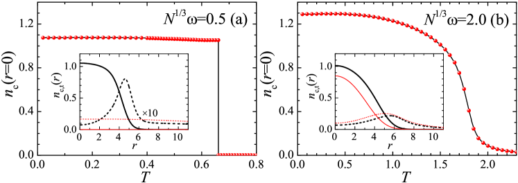
Figure 7: Temperature dependence of the central condensate density at $N^{1/3}\omega=0.5$ (a) and $N^{1/3}\omega=2.0$ (b). The insets show the condensate and thermal density distributions at $T=0.95T_{c}$ (black thick curves) and at $T=1.05T_{c}$ (red thin curves), respectively. The condensate distribution is plotted in solid line and the thermal distribution is in dashed line.

Appendix F Central condensate density across the superfluid transition

The difference in the first-order and second-order BEC transitions can be mostly easily identified by measuring the central condensate density at the trap center. In Fig. 7, we report the central condensate density as a function of temperature at two different effective trapping frequencies $N^{1/3}\omega=0.5$ (a) and $N^{1/3}\omega=2.0$ (b), at which the system experiences the first-order transition and second-order transition, respectively. The two insets show the spatial distributions of the condensate density and the thermal density before and after the BEC transition, see, for example, the black thick curves at $T=0.95T_{c}$ and the red thin curves at $T=1.05T_{c}$.

The first-order BEC transition is clearly revealed in the inset of Fig. 7(a), where the central condensate density suddenly jumps to zero, while the thermal density (enlarged by ten times in the inset) becomes nearly flat in the region plotted. In sharp contrast, at second-order BEC transition the central condensate density gradually vanishes as the temperature increases. As illustrated in the inset of Fig. 7(b), there is still a considerable condensate density at $T=1.05T_{c}$, due to the finite number of particles (i.e., the finite-size effect).