Early Detection of In-Memory Malicious Activity based on Run-time Environmental Features

Abstract

In recent years malware has become increasingly sophisticated and difficult to detect prior to exploitation [13]. While there are plenty of approaches to malware detection, they all have shortcomings when it comes to identifying malware correctly prior to exploitation. The trade-off is usually between false positives, causing overhead, preventing normal usage and the risk of letting the malware execute and cause damage to the target [22][14][21].
We present a novel end-to-end solution for in-memory malicious activity detection done prior to exploitation by leveraging machine learning capabilities based on data from unique run-time logs, which are carefully curated in order to detect malicious activity in the memory of protected processes. This solution achieves reduced overhead and false positives as well as deployment simplicity.
We implemented our solution for Windows-based systems, employing multi disciplinary knowledge from malware research, machine learning, and operating system internals. Our experimental evaluation yielded promising results. As we expect future sophisticated malware may try to bypass it, we also discuss how our solution can be extended to thwart such bypassing attempts.

1 Introduction

In recent years malware has become increasingly sophisticated and difficult to detect prior to exploitation[13], and there are different approaches that attempt to detect and protect against it prior to exploitation of the target, see e.g. [10][12][27]. Solutions include Endpoint Protection Platforms (EPP) such as legacy or next-generation anti-viruses, Endpoint Detection and Response (EDR), Managed Detection and Response (MDR), Cross-layered Detection and Response (XDR) and many more [5]. These solutions usually rely on either a constantly updated database of signatures for detecting malware variants that have already been seen in the wild, a predefined set of rules or heuristics for identifying malicious activity by actions taken by a program, leveraging more advanced machine learning techniques like behavioral analysis (to deduce if an entity or set of actions is malicious or not), or any hybrid combination of these approaches [18][24][33].

All these approaches have shortcomings when it comes to identifying malware correctly prior to exploitation. In some cases, if the resource defined as a potential target is very critical to the organization, e.g. a global authentication service running on a secure server, the owners will have a great incentive to protect it, but for most protection mechanisms this is likely to cause an increased number of false positives on accesses of the resource, an adverse impact on performance, or even hurting the functionality provided by the resource. All these potential problems often deter organizations from hardening the protection of critical resource in comparison with the rest of the system [15][3].

The end result is a similar protection level for all of the resources in the system which is often insufficient for protecting against very sophisticated malware, especially in-memory ones [28][20].

In this work, we describe a security mechanism that ensures, with high probability, that detection occurs in real time prior to any malicious action that impacts the attacked system.

Our solution was implemented by training a malware detection machine learning model on a large data-set of run-time logs (provided by Morphisec Ltd). These logs were collected from real-world machines during both standard workloads and real malware attacks. The logs contain a set of environmental and process-related variables we efficiently extract during run-time that were identified as important for the detection of in-memory attacks.
Using the deployed detector, our system is able to query a minimal run-time log from a critical process to infer if an in-memory malicious activity is about to take place and perform a mitigation action before any harmful operation is performed.

Numerous malware detection approaches exist [25][23][26][11][13][10][12][27][18][24][33]. Malware detection using ML models often analyzes the contents of files (e.g. executable files) or other data sources for extracting features to train the model [32][29][30][31][17][16], or transforms the problem to another domain, such as image recognition [38][35]. Unlike these approaches, our solution uses run time environment logs in a very efficient and seamless manner (in comparison to memory dump analysis or sandbox/VM approach [34][19][37][36]). In comparison to other solutions that monitor processes in real-time, our solution is non-intrusive and does not hurt system performance [22][14][21][15][3]. It also reduces false positives to a minimum based on a rating system, as a threshold is set depending on how early the detection is required, providing a trade-off between the length of the early warning interval and the rate of false positives.

The rest of this paper is organized as follows: In section 2 we describe our data set. In section 3 we showcase the high level pipeline for our model creation, features selection and describe the rational behind it. In section 4, we describe the high-level architecture of our detector. We report on our experimental evaluation in section 5. Finally, we discuss our conclusions and directions for future work in section 6.

2 Dataset

The dataset used in this research is composed of logs containing environmental information regarding a specific process, that are collected live at runtime.
The environmental information collected consists of both static data (that could have been collected without the execution of the process) and dynamic data collected from the virtual memory of the process itself.

The dataset spans logs from the entire year of 2019 (that is, between January 1, 2019 and December 31, 2019). These logs are from real world scenarios, real world incidents in actual production machines with real users using them on a daily basis to do their work.

The logs were collected using a proprietary agent program (provided by Morphisec Ltd). This proprietary software leverages deep integration in the operating system’s kernel in order to block malicious activity during runtime using various memory-morphing techniques. The logs are not part of the defense mechanism, we made use of these logs to further understand and analyse specific points in the life cycle of processes.

These logs are taken prior to exploitation, which means that any malicious activity has not yet taken place in the target machine, however, the malicious entity was indeed running.

There are two types of logs collected in the dataset:

1. Malicious activity: Environmental runtime logs from incidents where the following actions taken by the malicious entity were indeed malicious (e.g. a log from the starting point of a ransomware malware execution).

2. Benign activity: Environmental runtime logs from incidents where the application/process/service are benign and the following actions were non-malicious (e.g. opening a malware-free document file via Microsoft Word).

Using the proprietary deterministic solution to mark each log, means that all of the records in the dataset are already labeled as malicious or benign. These labels were reviewed regularly by malware analysts to further reduce the probability of false positives/negatives.

2.1 Data Analysis

Each log is unique, there are no two logs which are exactly the same.
Any identifiable information in the logs, such as usernames, machine names, domain names, etc. was anonymized in order to preserve privacy.
In Table 2 and Table 2 we present some statistics about the dataset.

Table 1: Dataset: Labels

Label	Count
Malicious	1,637,645
Benign	827,938
Total	2,465,583

Table 2: Dataset: Classification by type

Classification by malware	Count
Classified	1,043,520
Unclassified	594,125
Total (malicious)	1,637,645

As can be seen from Table 2, there is almost a 2:1 ratio between the malicious samples and the benign ones. As presented by Table 2, almost two thirds of the malicious samples are also classified by type (e.g. Trojan).

In Table 3 we present data showing that our data set is heterogeneous in terms of malware and attack types, operating systems, machines, users etc., thus the data is unlikely to cause over-fitting to any one of these characteristics.

Table 3: Dataset: Unique values

Parameter	Count
Unique Malware Types	+15
Unique Attacks	+100
Unique Operating Systems	+10
Unique Machines	+1M
Unique Users	+1M
Unique Domains	+100K
Unique IP Addresses	+1M
Unique Application/Process Names	+1000
Unique Thread Count	+20
Unique Loaded Modules Count	+500K

There are 20 malware categories in the dataset as classified by YARA rules. These categories are detailed by Table 4.

Table 4: Dataset: Malware categories

Malware Categories
Adware	Exploit Kit	Keylogger	Shellcode
Fileless	Vulnerability	Banking Trojan	Info Stealer
Rootkit	Code Injection	Miner	Backdoor
Spyware	Supply Chain	Ransomware	Trojan
Virus	Hacking Tool	Worm	Remote Code Execution

2.2 Log Structure

The records in the dataset are basically documents in JSON format, resembling runtime logs containing a predetermined set of fields holding environmental data about a certain process under observation. The log files contain a lot of textual information. Nevertheless, their size is typically quite small, peaking at 500KB.

There are dozens of different fields and attributes as part of the log specification (which is proprietary), however, we chose only the most relevant fields in the logs, detailed in Appendix G, which are also available to be collected during runtime using open source tools and/or low level coding.

3 Pre-Processing and Model Generation

The essence of the solution lays in the machine learning model trained on a big data set of real-world logs representing malicious activity in various execution stages and from various types of malware, as well as benign data from standard applications.

3.1 High-level flow

The high level flow of the model training procedure is as follows (see Figure 1):

1. Given a data set of logs in the correct format, extract the textual features required and convert them from textual representations to numeric vectors using a standard Natural Language Processing algorithm, do this for every value (i.e. a full word) in the logs.

2. Given a data set of logs represented as numeric vectors (that is, the output from the previous stage), convert each log file containing these numeric representations to a single numeric vector, using a standard calculation from the world of document classification.

3. Given a set of numeric vectors to be used as a training set with proper labels (either malware or benign), train a prediction model in a supervised manner, using a standard Machine Learning ensemble approach from the world of classification.

Figure 1: Pre-Processing and Model Generation: Model training process

We describe the training process in more detail in the following sub-sections.

3.2 Data Preparation

In this stage, we did the following:

1. Cleaned the data where it was needed using Python scripting over the JSON documents:

   1. Dealing with wrong data types (e.g. text instead of integer) by removing it altogether.

   2. Dealing with missing values, keep them as is (empty), as long as most of the log itself still contains proper values.

   3. Normalizing numeric values that were out of the range expected for certain fields, taking the average from the same classification group if possible.

   4. Correcting errors in parsing in case of incorrect syntax, etc.

2. Shuffling of the logs in order to avoid any existing patterns in the way they will be split to sets.

3. We split the data set according to the ”Holdout method” to a training set, which also acts as a validation set, and a testing set, ahead of time. The dataset we use, whose dimensions are presented in Table 2, consists of the instances of the test set (set aside initially and consisting of an equal number of malicious and benign instances) and a subset of the remaining instances of a larger collection of instances from 2019. The proportion between malicious and benign training set instances was selected so as to optimize the AUC of our cross-validation tests on the training set. The best cross validation results were obtained when the proportion of malicious instances in the training set is approximately 70%, as shown by Table 5.

   Table 5: Pre-Processing and Model Generation: Split to sets

   Set	Malicious	Benign	Total
   Training	1,336,432	526,725	1,863,157
   Test (Holdout)	301,213	301,213	602,426

4. Prepared the high-performance training server, placing the relevant sets of documents ready to be input to the next stage in the process.

3.3 Feature Engineering

The main strength of our model lays in its features chosen carefully from the logs as each and every one of them contributes in the detection process.

We chose approximately 40 features, consisting of metadata fields (Appendix G.2), runtime-related features (Appendix G.3), and PE-related fields (Appendix G.4) (see sub-section 2.2). Anonymized features (Appendix G.1) were not selected. The full list of features is presented in Appendix G.

3.4 Textual Features to Associations

After extracting the features, we wanted to understand what is the similarity between all their values in the set that we received. As the features have textual representation we decided to leverage this and use a well-known method from the field of Natural Language Processing, called word2vec.

This method uses a shallow two-layered neural network to process and convert every value (’word’) in the log to a meaningful one-dimensional vector of size 32. Using word2vec, values (’words’) with similar context should have a similar vector as given by measuring cosine similarity between values.
We wanted a simple pre-tweaked black box solution for the word embedding, so we tested both of the popular options: word2vec [8] and FastText[2], there were only minor differences between them in terms of the resulting detection quality, so we chose to use word2vec.

In Figure 2, we can see an example of the most similar vectors for the vector representing the string ”kernel32.dll” from the feature ”list of loaded modules”.

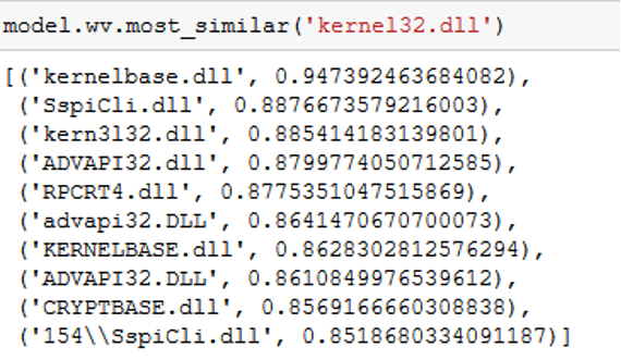
Figure 2: Pre-Processing and Model Generation: Vector value for ”kernel32.dll”

In Figure 3, we can see an example of the most similar vectors for the vector representing the string ”LoadLibraryA” which is a common Win32 API function used by both malware and benign applications.

Figure 3: Pre-Processing and Model Generation: Vector value for ”LoadLibraryA”

The word2vec model is trained in an unsupervised manner, which means we ignore the labels (benign, malicious), and provide a vector for each and every unique feature value in the training set.

3.5 Dimensionality Reduction

After the word2vec model is trained, we need to convert every log as a whole to a representative vector that we can work with. For this purpose we use a common method usually used for document classification tasks, which allows us to reduce the dimension of the log while preserving semantics.

For each of the following types of features, we calculated the mean vector of all the vectors (that we received as an output from the word2vec model) that represents the values (’words’) inside them using Python scripting:

1. Stack snapshot and trace

2. Registers data, opcodes collected in memory

3. Loaded modules and resources

4. Process and metadata information (e.g. parent process and OS version, respectively)

This produces a one-dimensional vector of size 192 for every specific log. This vector is then used as input for a supervised classifier to be trained in the next stage.

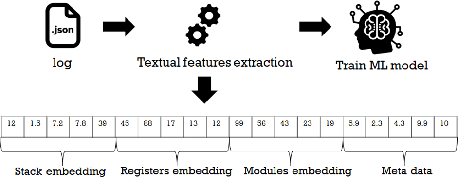
Figure 4: Pre-Processing and Model Generation: log2vec

Figure 4 illustrates the process of transforming a single log to a one-dimensional vector using the vectors we got from word2vec, as well as an example of how this vector is organised.

3.6 Training

Now that we have all the logs represented as one-dimensional vectors in the training set, we can input them as training data with their labels, to an ML algorithm trained in a supervised manner.
We chose the gradient boosting technique which outputs a prediction model in the form of an ensemble of weak prediction models (in our case, decision trees [6]).
We wanted a simple pre-tweaked black box solution for gradient boosting, so we tested both of the popular options: XGBoost [9] and LightGBM [7]. Since there were only minor differences between them in terms of detection quality, we chose LightGBM which was easier to use.

4 Detection Framework

4.1 Architecture

Our detection framework consists of the following parts:

I. ”Detector”: A novel machine learning model trained on a big data set of environmental run-time logs captured from real-world malicious incidents per a specific protected process. This model runs on a standard server in the cloud, receives a log for detection and replies with a relative score, quantifying the probability that the activity represented by the log is malicious.

II. ”Agent”: A lightweight service running on the endpoint machine whose task is to generate log instances from critical processes that are to be protected and send them to the Detector over the network.

4.2 High level flow

1. A critical process, which should be protected, is running on the endpoint machine, a lightweight log extraction service is installed and extracts logs during run-time as required.

2. The extracted log is sent from the endpoint machine to the Detector server for detection.

3. The Detector server inputs the received log into the already-deployed machine learning model to receive a detection score.

4. A result with a score for the activity diagnosed from the given log, is being sent from the server to the endpoint for taking further actions as needed.

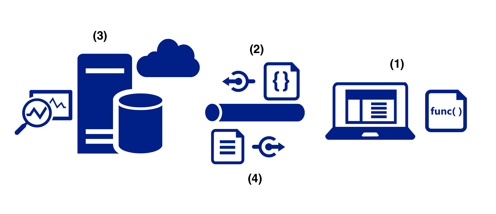
Figure 5: Detection Framework: High Level Flow.

5 Experimental Evaluation

In this section, we describe the experimental evaluation we conducted to assess the quality of our detection framework and its results.

5.1 Experiment 1: Detection Model Confusion Matrix

Our evaluation uses the test set defined in section 3. The results are presented by Table 6 and Figure 6. These results were obtained by using a classification threshold of 0.75.

Table 6: Experimental Evaluation: Confusion Matrix for the test set

	Positive (predicted)	Negative (predicted)
Positive (actual)	301,202	11
Negative (actual)	111	301,102

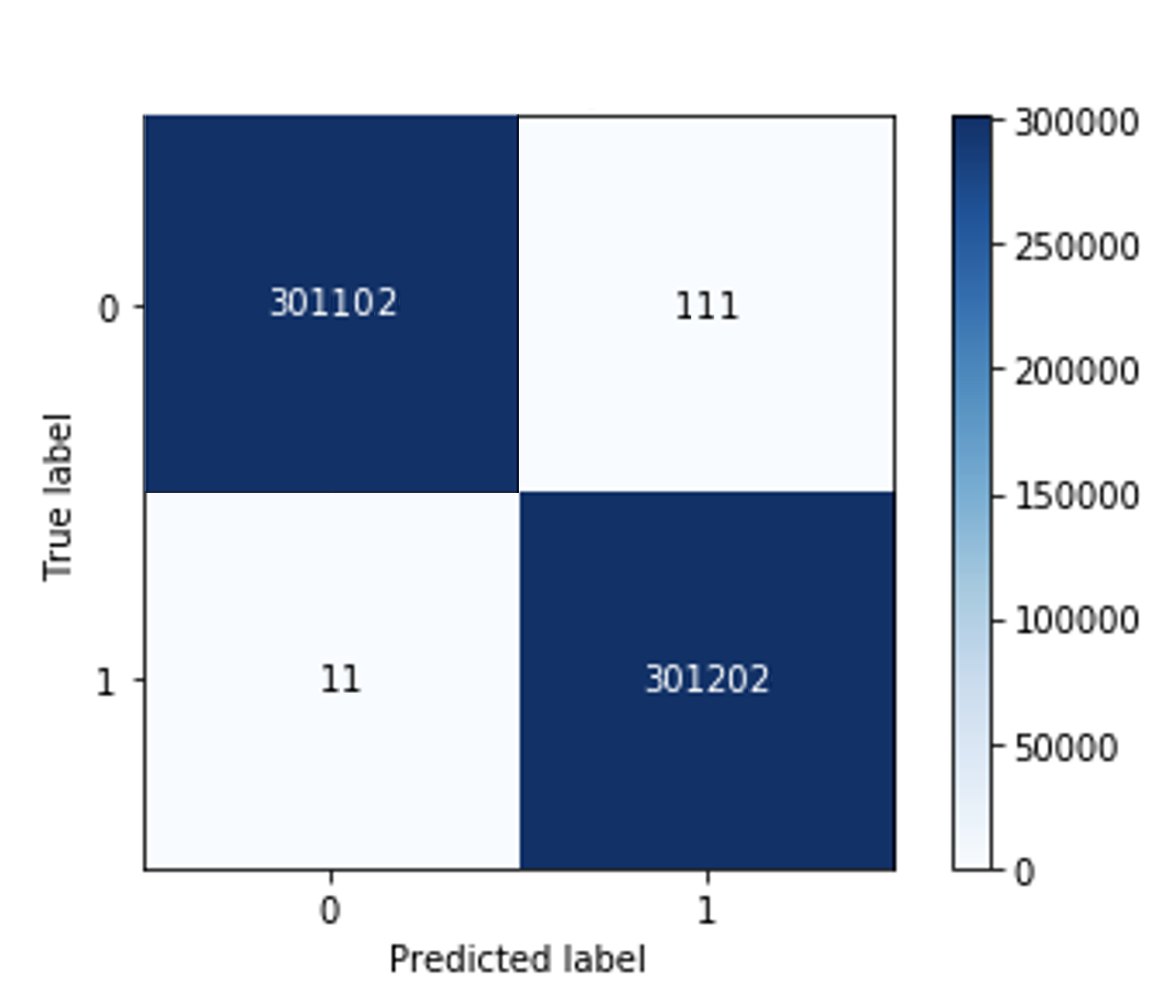
Figure 6: Experimental Evaluation: Confusion heatmap

Other metrics that are computed based on the confusion matrix are shown in Table 7.

Table 7: Experimental Evaluation: Metrics for the test set

Metric	Value
Area Under the ROC Curve (AUC)	0.997712
Accuracy (ACC)	0.999797
Precision (PPV)	0.999632
Recall (TPR)	0.999963
False Positive Rate (FPR)	0.000369
False Negative Rate (FNR)	0.000037
F1 Score	0.999798

As presented by Table 7, detection quality is very high. Specifically, the recall is nearly 1 while the FPR is extremely low, approximately 0.04%.

5.2 Experiment 2: Testing Benign Applications

We already tested our solution using logs from the dataset that represent benign processes, however, we wanted to simulate a real-world scenario with a typical machine in an organisation, running a mixture of productivity applications, collaboration tools, etc., in parallel.

For this endeavour, we installed a pre-defined set of benign applications on a Windows 10 64-bit machine, all of them are either mainstream applications intended for daily use, or already built in the operating system.

As the list contains 30+ applications, it is included in Appendix H. We covered all of these applications using our Agent service, collecting logs intermittently, and assessing the results returned from the Detector in real time.

Using the same 0.75 classification threshold, we placed the 184 results in a confusion heatmap . As seen in Figure 7, results are very good, having only 2 logs as false-positives, as 181 of the logs were classified correctly as benign.

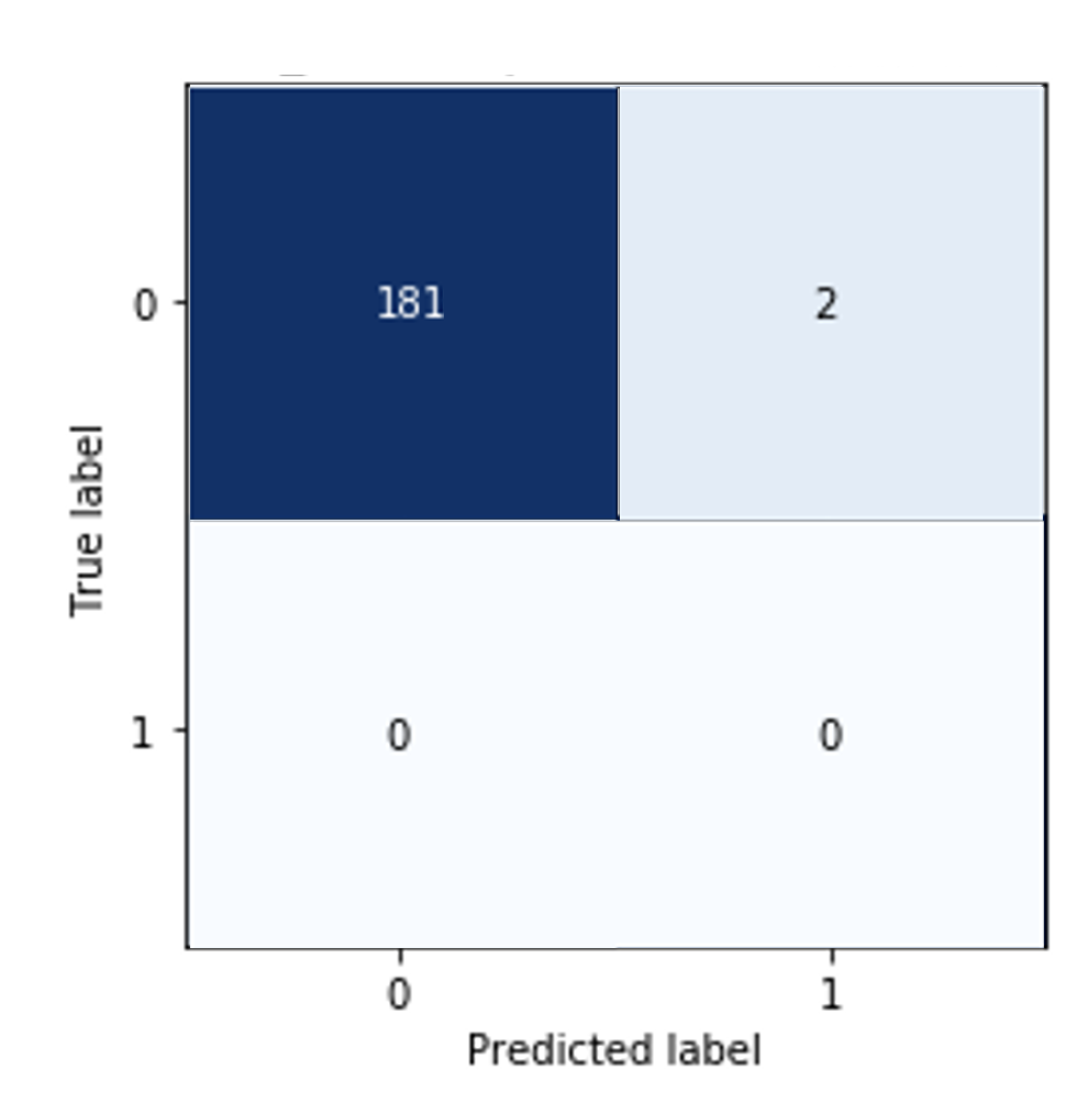
Figure 7: Experimental Evaluation: Benign applications

5.3 Experiment 3: Testing Malicious Applications

In this experiment, we simulated a real-world scenario with a typical machine in an organisation, infected by malware from different types.

For this endeavour, we used an automation environment (Cuckoo sandbox [1]) to run malware on a Windows 10 virtual machine, while the Agent service is also running to collect logs.

As the list contains 40+ examples of different malware, it is included in Appendix I, sorted by categories. We repeated the experiment for each of these malicious programs.

Using the same 0.75 classification threshold, we placed the 220 results in a confusion heatmap. As can be seen in Figure 8, only 2 logs were misclassified as false negatives, whereas 218 of the logs were correctly classified as malicious.

Figure 8: Experimental Evaluation: Malware

5.4 Experiment 4: Analyzing Performance

In order to assess how efficient our Agent is and if it causes any noticeable degradation in overall system performance, we conducted two tests:

1. Running standard applications typically used by enterprise users, with and without the Agent coverage for these applications, for a few hours, while collecting logs intermittently.

2. Calculating the amount of CPU and memory usage for the Agent service while continuously collecting logs.

The list of applications tested can be viewed in Table 8, the resulting performance graphs appear in Appendix J.

Table 8: Experimental Evaluation: Applications tested for performance

Application
Microsoft Excel 2016	Acrobat Reader DC
Microsoft PowerPoint 2016	Skype (8.55)
Microsoft Word 2016	Internet Explorer 11
Microsoft Outlook 2016	Google Chrome (v78)

According to our testing, if we ignore the outliers, there was no noticeable overhead running the applications in test with the agent compared to running them without the Agent.

As the Agent’s CPU utilization is always below 100%, it is using one logical CPU core at most. In addition, the Agent’s memory usage never exceeded 25MB, which is reasonably low on contemporary commodity computers.

6 Conclusion

As malware rose in sophistication and volume in recent years, so is the requirement for innovative solutions for its detection. In this work we presented an end to end ML-based solution for the early detection of in-memory malicious activity via runtime logs, to demonstrate the potential of leveraging the plethora of process and environment data that can be collected from processes executing on endpoint machines over time and be used for malware detection. Our experimental evaluation establishes that this approach has the potential of yielding high-quality detection of malicious process activity before it performs harmful operations.
In future work, we plan to investigate the length of the early warning period that can be achieved using our detection approach, that is, how long before the malware attempts to execute its harmful operations can it be detected using our approach. In addition, there are challenges yet to be overcome regarding our solution’s limitations, these include: reducing the downtime on update, minimizing compatibility issues on the Agent’s side, attempting to provide offline detections, overcoming the performance limitation of parallel logging and the overhead stemming from retraining of the model. Additional avenues for future research include extending our detector by improving the server-side component, security, communications, anti tampering, and logging mechanisms.

Appendix G Logs

In this appendix, we list the log fields used as features in sub-section 3.3.

Appendix G.1 Anonymized

The following fields contain personal information and are anonymized in advance:

1. Username of the user logged in (if there is an interactive user logged in) at the time of the incident.

2. Domain name the target machine belongs to (if there is one).

3. Machine name of the target machine.

4. IP address of the target machine.

5. Machine serial number if the machine is prebuilt by a vendor or an OEM (e.g. a laptop).

Appendix G.2 Metadata

The following fields are considered metadata:

1. Timestamp of the incident, Date/Time in milliseconds.

2. Operating System of the target machine, in our case, a version of Windows (e.g. Windows 7 32-bit).

3. Operating System build number

4. Executable full path for the executable whose code the process under observation is executing.

5. Executable name.

6. Executable hash.

7. File attributes Creation time and modification time of the executable.

8. Referral URL from where the executable was downloaded, if it was downloaded off the internet.

9. User login time of the last logged in user.

10. Thread count for running threads in the process.

11. Integrity level of the process, can be Untrusted, Low, Medium, High or System. This defines the trust level for this process in Windows based systems.

12. Executable architecture whether it is 32 or 64 bit.

13. Total work time done for the process so far in both processor clock cycles and in process time done in kernel mode.

14. Process ID of the executable.

15. Thread ID of the thread executing the monitored code within the process.

16. User privilege level for the currently logged in user, if there is one, allows distinguishing between Standard users, Guests and Administrators.

17. Timezone of the target machine at the time of the incident.

Appendix G.3 Runtime

The following fields are considered essential information for understanding the incident and are collected from the environment and the process itself during runtime:

1. Base address starting from which the executable was mapped into memory.

2. Command line arguments used for running the executable.

3. Value of all the registers, that is, a the current contents of EAX, EBX, ECX, EDX, EBP, ESP, EDI, ESI, etc. for the currently executing thread in the process.

4. Snippets of bytes pointed to by all the registers, that is, a snapshot of the bytes pointed by the addresses in registers EAX, EBX, ECX, EDX, etc. if these are valid addresses in memory, for the current executing thread (although the heap, code and data are shared across the process).

5. EFLAGS register contents for the currently executing thread in the process.

6. Digital certificate / signature of the executable.

7. List of loaded resources by the executable, and their properties: full path, size, hash, creation time, modification time.

8. Amount of virtual memory both free and used in bits.

9. Specific information from HKLM registry values including ”run” and ”runonce” key-value pairs.

10. DEP protection status at the time of the incident.

11. List of illegal addresses in the virtual memory the executable tried to access and snippets of bytes from these addresses, hopefully translating into opcodes.

12. Hash of the import table from the PE file.

13. Details about the injecting process, if there is one (e.g. remote thread injection), details include: process ID, parent process ID, hash, full path to executable.

14. Flag indicating if the executable has the auto-elevation property in its manifest. This property is typically used for running at a higher privilege level in order to bypass the User Account Control on Windows systems.

15. List of loaded modules at the time of the incident, including details for each one: base address in memory, end address in memory, size, file linking metadata and full path to the module.

16. List of opened resources by the process in the time of the incident, for example, file handles, and the attributes of these files.

17. Details about the parent process of the executable, including process ID, full path, hash, file attributes, command line arguments used to run the parent process, integrity level, resources with their details, loaded modules and opened resources.

18. List of process block data from the executable up to the first unprotected parent process.

19. Snapshot of the stack’s memory and stack trace at the time of the incident for the current executing thread.

20. List of files by their magic if found in the process’s memory, e.g. PDF or script files in the memory of the process.

21. List of URLs, if found, using a regex search in the process’ memory.

22. List of IP addresses, if found, using a regex search in the process’ memory.

23. List of task scheduler tasks if they are related to the executing process.

24. List of registry change attempts and their results in certain regions of the registry.

Appendix G.4 PE

The following fields are extracted from the PE file itself, if possible:

1. PE type

2. Section count

3. Section information

4. Import count

5. Import information

6. Export count

7. Export information

8. Executable export name

9. Characteristics

10. Compilation time

11. Executable signature

12. Executable architecture

13. Entry point

14. Entropy level

15. Executable size

16. PDB path

17. Executable Creation time

18. Executable Modification time

Appendix G.5 Example

In Figure 9 we can see an example of a partial log file collected in real time for a Mimikatz credential theft attack, which is considered an info stealing malware[4].

Figure 9: Appendix G: Log example

Appendix H Benign Applications List

In this appendix, we list the benign applications being used for testing in sub-section 5.2, by category.

1. Collaboration applications are listed in Table 9, 7 applications in total.

2. Productivity and media applications are listed in Table 10, 16 applications in total.

3. Applications used for executing code are listed in Table 11, 10 applications in total.

Table 9: Appendix H: Collaboration applications

Application	Usage	Executable Name
Cisco WebEx	Virtual conferencing	webex.exe
GoToMeeting	Virtual conferencing	gotomeeting.exe
Skype	Voice-over-IP	skype.exe
Slack	Instant messaging	slack.exe
Microsoft Teams	Virtual conferencing	teams.exe
TeamViewer	Screen sharing	teamviewer.exe
Zoom	Virtual conferencing	zoom.exe

Table 10: Appendix H: Productivity and media applications

Application	Usage	Executable Name
Acrobat Reader	PDF viewer	acrord32.exe
Microsoft Excel	Spreadsheet editor	excel.exe
Microsoft Word	Document editor	word.exe
Microsoft PowerPoint	Presentation editor	powerpnt.exe
Microsoft Access	Database management	msaccess.exe
Microsoft Outlook	Email client	outlook.exe
Google Chrome	Web browser	chrome.exe
Mozilla Firefox	Web browser	firefox.exe
Microsoft Internet Explorer	Web browser	iexplore.exe
Microsoft Edge	Web browser	msedge.exe
VideoLAN (VLC)	Media player	vlc.exe
7-Zip	File archiver	7z.exe
WinRAR	File archiver	winrar.exe
FortiClient	VPN	forticlient.exe
Task Manager	Scheduled tasks	taskeng.exe
Registry Editor	Windows Registry	regsvr32.exe

Table 11: Appendix H: Code-execution applications

Application	Usage	Executable Name
AutoIt	AutoIt V3 scripts	autoit3.exe
Java RTE	Java code	java.exe
Python 3	Python code	python3.exe
NodeJS	NodeJS applications	node.exe
Cscript	VBscript / WSH script	cscript.exe
MSHTA	Microsft HTML applications	mshta.exe
Rundll32	Load DLLs	rundll32.exe
Wscript	Windows Script Host	wscript.exe
PowerShell	PowerShell scripts	powershell.exe
CMD	Command prompt	cmd.exe

Appendix I Malicious Applications List

In this appendix, we list the malware being used for testing in sub-section 5.3, by category, using either their common name or their CVE.

1. Malware exploiting the target system via PDF files, opened via Acrobat Reader, are listed in Table 12, 8 attacks in total.

2. Malware exploiting the target system via docx or xlsx files, opened via Microsoft Word or Excel, are listed in Table 13, 15 attacks in total.

3. Malware exploiting the target system via VB, Flash or Silverlight, are listed in Table 14, 30 attacks in total.

4. Exploit kits are listed in Table 15, 8 exploit kits in total.

5. Ransomware are listed in Table 16, 43 attacks in total.

6. Various other malware are listed in Table 17, 56 attacks in total.

Table 12: Appendix I: PDF malware

CVE
CVE-2014-0496	CVE-2013-0640	CVE-2010-2883
CVE-2013-3346	CVE-2013-2729	CVE-2010-0188
CVE-2012-0754	CVE-2011-2462

Table 13: Appendix I: docx/xlsx malware

CVE
CVE-2017-11882	CVE-2017-11826	CVE-2017-0262	CVE-2015-5119
CVE-2015-2545	CVE-2015-1770	CVE-2014-1761	CVE-2013-3906
CVE-2012-0158	CVE-2012-2539	CVE-2012-0158	CVE-2012-1642
CVE-2012-0158	CVE-2009-3129	CVE-2010-3333

Table 14: Appendix I: VB/Flash/Silverlight malware

CVE
CVE-2018-15982	CVE-2018-8174	CVE-2018-4878
CVE-2017-11292	CVE-2015-7645	CVE-2015-5560
CVE-2015-5122	CVE-2015-5119	CVE-2015-3113
CVE-2015-3105	CVE-2015-3104	CVE-2015-3090
CVE-2015-0359	CVE-2015-0336	CVE-2015-0313
CVE-2015-0311	CVE-2014-8439	CVE-2014-0569
CVE-2014-0556	CVE-2014-0515	CVE-2014-0497
CVE-2013-3897	CVE-2013-3893	CVE-2013-3163
CVE-2013-2551	CVE-2013-1347	CVE-2012-4792
CVE-2012-1876	CVE-2012-1875	CVE-2011-1996

Table 15: Appendix I: Exploit kits

Name
Angler	Nuclear
Fiesta	RIG
Magnitude	Sundown
Neutrino	Sweet Orange

Table 16: Appendix I: Ransomware

Name
Ryuk	Ransomware-X	RagnarLocker	Snake (Go)	Thanos
MedusaLocker	PonyFinal (Java)	REvil	Bandarchor	BTCware
Cerber	NewCerber	Cobra-Crysis	CoinMiner	CryptFile2
CryptoMix	CryptoLocker	CryptoWall	CryptoShield	CryptXXX
Gandcrab	Dharma-AUDIT	GlobeImposter	Gryphon	Jaff
JagerDecryptor	Locky	Osiris	Magniber	Matrix
Mole	Petya, Mischa	Philadelphia	Santa	Satan
SAVEFiles	Sega2.0	Shade	Sigma	Spora
TeslaCrypt	WannaCry	XData

Table 17: Appendix I: Various malware

Name	Category	Name	Category	Name	Category
Andromeda	Bot	Bunitu Proxy	trojan	Chthonic	Banking trojan
AZORULT	Spyware	BetaBot	Info stealer	BitCoinMiner	Miner
Corebot	Banking trojan	Cridex	Bot, Info stealer	Cutwailpushdo	Bot
DanaBOT	Bot	Dreambot-Ursnif	Banking trojan	Dridex	Info stealer
Emotet	Trojan	Flawed Ammyy	RAT	FlokiBot	Banking trojan
Formbook	Trojan	Godzilla	Loader	Graybird	Backdoor
IcedID	Banking trojan	Imminent	RAT	ISRstealer	Info stealer
Kasidet-Neutrino	Bot	Kovter	Fileless	Kronos	Banking trojan
LatentBot	RAT	LokiBot	Banking trojan	Neurevt	Info stealer, Bot
NSIS-injector	Trojan	PlugX	RAT	Pony	Info stealer
Potao Express	Toolkit	Poweliks	Fileless	Pushdo	Bot
QBot	Bot	Quant	Loader	Ramnit	Banking trojan
Redaman	Banking trojan	Remcos	RAT	RokRAT	RAT
Rombertik	Spyware	SmokeLoader	Bot	Snatch	Loader
SpyWare	Rootkit	Terdot.A	Trojan	Zloader	Loader
Tesla	Keylogger	TrickBot	Trojan	Trojan—pzamd	Trojan
Uptare	Trojan	Ursnif	Banking trojan	Vawtrak	Banking trojan
XMRig	Miner	ZeroAccess	Trojan	Zeus Panda	Banking trojan
ZeusVM	Banking trojan

Appendix J Performance

In this appendix, we provide the results of the performance analysis done for the Agent.
Figure 10 presents Microsoft Office applications (e.g. Word) running with and without the Agent coverage.

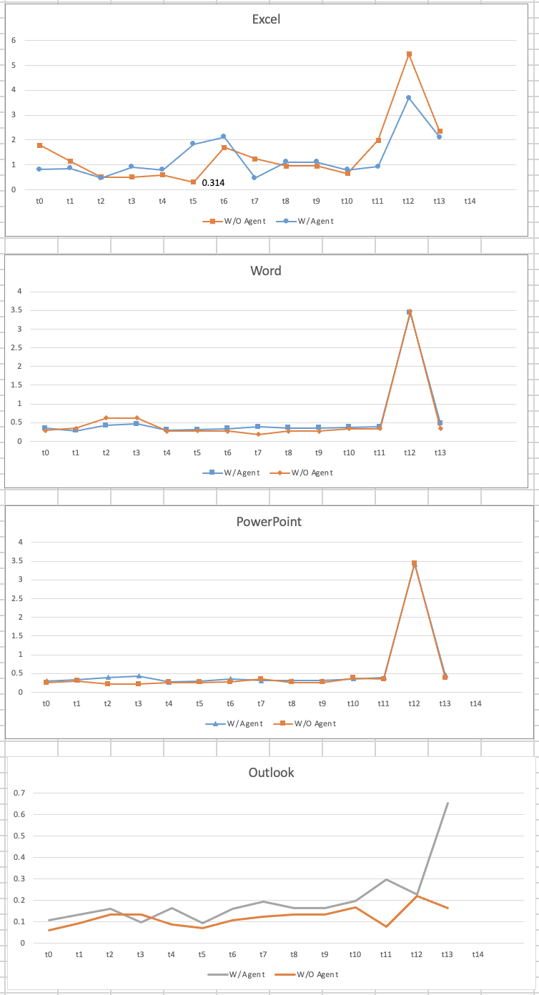
Figure 10: Appendix J: Microsoft Office applications with and without Agent coverage

Figure 11 presents various applications (e.g. Google Chrome), running with and without the Agent coverage.

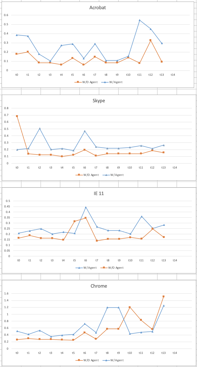
Figure 11: Appendix J: Various applications with and without Agent coverage

Figure 12 presents the amount of CPU usage and memory usage for the Agent service while it is collecting logs in a continuous matter. The Y-axis of the CPU chart is the percentage of CPU utilization at time t (the X-axis). The Y-axis of the Memory Usage chart is the peak amount of physical RAM allocated to the Agent at time t (the X-axis).

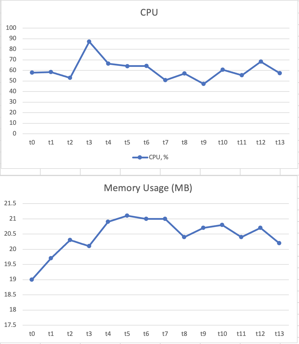
Figure 12: Appendix J: CPU and Memory Usage

The tests were conducted using Microsoft Windows Performance Toolkit (aka Xperf), on the same baseline machine having the following specifications:

1. OS: Windows 10 x64

2. CPU: Intel 4-Cores

3. RAM: 8GB DDR4

4. SSD: 256GB SATA3

References

- [1] Cuckoo sandbox (Dec 2020), https://cuckoosandbox.org/
- [2] Fasttext (Dec 2020), https://fasttext.cc/
- [3] Meeting the challenges of endpoint security, whitepaper, (Oct 2020), https://www.cstl.com/utils/downloads/Symantec-Hosted-Endpoint-Whitepaper.pdf
- [4] Mimikatz credential theft (Dec 2020), https://www.crowdstrike.com/blog/credential-theft-mimikatz-techniques/
- [5] Understanding mdr, edr, epp and xdr (Oct 2020), https://www.netsurion.com/articles/understanding-mdr-edr-epp-and-xdr
- [6] Wikipedia: Decision tree learning (Dec 2020), https://en.wikipedia.org/wiki/Decision_tree_learning
- [7] Wikipedia: Lightgbm (Dec 2020), https://en.wikipedia.org/wiki/LightGBM
- [8] Wikipedia: Word2vec (Dec 2020), https://en.wikipedia.org/wiki/Word2vec
- [9] Wikipedia: Xgboost (Dec 2020), https://en.wikipedia.org/wiki/XGBoost
- [10] Aslan, Ö.A., Samet, R.: A comprehensive review on malware detection approaches. IEEE Access 8, 6249–6271 (2020)
- [11] Birman, Y., Hindi, S., Katz, G., Shabtai, A.: Cost-effective malware detection as a service over serverless cloud using deep reinforcement learning. In: 2020 20th IEEE/ACM International Symposium on Cluster, Cloud and Internet Computing (CCGRID). pp. 420–429. IEEE (2020)
- [12] Chakkaravarthy, S.S., Sangeetha, D., Vaidehi, V.: A survey on malware analysis and mitigation techniques. Computer Science Review 32, 1–23 (2019)
- [13] Erdődi, L., Jøsang, A.: Exploitation vs. prevention: The ongoing saga of software vulnerabilities. Acta Polytechnica Hungarica 17(7) (2020)
- [14] Hăjmăşan, G., Mondoc, A., Creţ, O.: Dynamic behavior evaluation for malware detection. In: 2017 5th International Symposium on Digital Forensic and Security (ISDFS). pp. 1–6. IEEE (2017)
- [15] Hăjmăşan, G., Mondoc, A., Portase, R., Creţ, O.: Performance improvements in behavior based malware detection solutions. In: IFIP International Conference on ICT Systems Security and Privacy Protection. pp. 370–384. Springer (2018)
- [16] Ijaz, M., Durad, M.H., Ismail, M.: Static and dynamic malware analysis using machine learning. In: 2019 16th International bhurban conference on applied sciences and technology (IBCAST). pp. 687–691. IEEE (2019)
- [17] Irshad, A., Maurya, R., Dutta, M.K., Burget, R., Uher, V.: Feature optimization for run time analysis of malware in windows operating system using machine learning approach. In: 2019 42nd International Conference on Telecommunications and Signal Processing (TSP). pp. 255–260. IEEE (2019)
- [18] Irshad, M., Al-Khateeb, H.M., Mansour, A., Ashawa, M., Hamisu, M.: Effective methods to detect metamorphic malware: a systematic review. International Journal of Electronic Security and Digital Forensics 10(2), 138–154 (2018)
- [19] Jamalpur, S., Navya, Y.S., Raja, P., Tagore, G., Rao, G.R.K.: Dynamic malware analysis using cuckoo sandbox. In: 2018 Second international conference on inventive communication and computational technologies (ICICCT). pp. 1056–1060. IEEE (2018)
- [20] Kumar, S., et al.: An emerging threat fileless malware: a survey and research challenges. Cybersecurity 3(1), 1–12 (2020)
- [21] Lungana-Niculescu, A.M., Colesa, A., Oprisa, C.: False positive mitigation in behavioral malware detection using deep learning. In: 2018 IEEE 14th International Conference on Intelligent Computer Communication and Processing (ICCP). pp. 197–203. IEEE (2018)
- [22] Marculet, D.G., Benchea, R., Gavrilut, D.T.: Methods for training neural networks with zero false positives for malware detection. In: 2019 21st International Symposium on Symbolic and Numeric Algorithms for Scientific Computing (SYNASC). pp. 230–236. IEEE (2019)
- [23] Mirza, Q.K.A., Awan, I., Younas, M.: Cloudintell: An intelligent malware detection system. Future Generation Computer Systems 86, 1042–1053 (2018)
- [24] Naz, S., Singh, D.K.: Review of machine learning methods for windows malware detection. In: 2019 10th International Conference on Computing, Communication and Networking Technologies (ICCCNT). pp. 1–6. IEEE (2019)
- [25] Nigam, P.: Malware detection and signature generation (2020)
- [26] Niveditha, V., Ananthan, T., Amudha, S., Sam, D., Srinidhi, S.: Detect and classify zero day malware efficiently in big data platform. International Journal of Advanced Science and Technology 29(4s), 1947–1954 (2020)
- [27] Or-Meir, O., Nissim, N., Elovici, Y., Rokach, L.: Dynamic malware analysis in the modern era—a state of the art survey. ACM Computing Surveys (CSUR) 52(5), 1–48 (2019)
- [28] Patten, D.: The evolution to fileless malware, [accessed on oct 2020] http://www.infosecwriters.com/papers/dpatten_fileless.pdf (2017)
- [29] Sethi, K., Chaudhary, S.K., Tripathy, B.K., Bera, P.: A novel malware analysis framework for malware detection and classification using machine learning approach. In: Proceedings of the 19th International Conference on Distributed Computing and Networking. pp. 1–4 (2018)
- [30] Sethi, K., Kumar, R., Sethi, L., Bera, P., Patra, P.K.: A novel machine learning based malware detection and classification framework. In: 2019 International Conference on Cyber Security and Protection of Digital Services (Cyber Security). pp. 1–4. IEEE (2019)
- [31] Sethi, Kamalakanta, S.K.C.B.K.T., Bera., P.: ”a novel malware analysis framework for malware detection and classification using machine learning approach.”. In: In Proceedings of the 19th International Conference on Distributed Computing and Networking. pp. 1–4. ACM (2018)
- [32] Sihwail, R., Omar, K., Ariffin, K.Z.: A survey on malware analysis techniques: Static, dynamic, hybrid and memory analysis. International Journal on Advanced Science, Engineering and Information Technology 8(4-2), 1662 (2018)
- [33] Souri, A., Hosseini, R.: A state-of-the-art survey of malware detection approaches using data mining techniques. Human-centric Computing and Information Sciences 8(1), 3 (2018)
- [34] Tien, C.W., Liao, J.W., Chang, S.C., Kuo, S.Y.: Memory forensics using virtual machine introspection for malware analysis. In: 2017 IEEE Conference on Dependable and Secure Computing. pp. 518–519. IEEE (2017)
- [35] Venkatraman, S., Alazab, M., Vinayakumar, R.: A hybrid deep learning image-based analysis for effective malware detection. Journal of Information Security and Applications 47, 377–389 (2019)
- [36] Walker, A., Amjad, M.F., Sengupta, S.: Cuckoo’s malware threat scoring and classification: Friend or foe? In: 2019 IEEE 9th Annual Computing and Communication Workshop and Conference (CCWC). pp. 0678–0684. IEEE (2019)
- [37] Wang, C., Ding, J., Guo, T., Cui, B.: A malware detection method based on sandbox, binary instrumentation and multidimensional feature extraction. In: International Conference on Broadband and Wireless Computing, Communication and Applications. pp. 427–438. Springer (2017)
- [38] Zhang, J., Qin, Z., Yin, H., Ou, L., Hu, Y.: Irmd: malware variant detection using opcode image recognition. In: 2016 IEEE 22nd International Conference on Parallel and Distributed Systems (ICPADS). pp. 1175–1180. IEEE (2016)