On the Predictability of Utilizing Rank Percentile to Evaluate Scientific Impact

Abstract

Bibliographic metrics are commonly utilized for evaluation purposes within academia, often in conjunction with other metrics. These metrics vary widely across fields and change with the seniority of the scholar; consequently, the only way to interpret these values is by comparison with other academics within the same field who are of similar seniority. Among the field- and time- normalized indicators, rank percentile has grown in popularity, and it is preferred over other types of indicators. In this paper, we propose and justify a novel rank percentile indicator for scholars. Furthermore, we emphasize on the time factor that is built into the rank percentile, and we demonstrate that the rank percentile is highly predictable. The publication percentile is highly stable over time, while the scholar percentile exhibits short-term stability and can be predicted via a simple linear regression model. More advanced models that utilize extensive lists of features offer slightly superior performance; however, the simplicity and interpretability of the simple model impose significant advantages over the additional complexity of other models.

Introduction

Comparisons of the scientific impact of scholars or publications often occur when making academic decisions. For instance, academic committees evaluate a candidate scholar relative to other cohorts in the same department to award tenure promotions. Directly comparing the number of citations can introduce bias, since the citations change with the seniority of the scholar. Another example is assigning research funding in which the scholar’s portfolio is compared to other candidates from various facilities and disciplines. The magnitude of the citations that a publication receives varies drastically across disciplines; consequently, utilizing citations favors scholars from more active fields and hence is not an appropriate measure.

Rank percentile, a popular field- and time-normalized indicator, has been studied extensively in the application of comparing scientific impacts. When applied to the evaluation of a publication, it normalizes the citations that the publication has received by its rank relative to other publications in the benchmark, and the benchmark specifies a field or publication year. The rank percentile has a significant advantage over other types of normalized indicators: for instance, a mean-based indicator normalizes the citations of publications in the benchmark with respect to the expected citation impact of the benchmark, which can be estimated by the arithmetic mean of citations for all publications in the benchmark [1]. Since the citation distribution is skewed and heavy-tailed, the arithmetic mean is not a reasonable representation of the expected citation impact, and therefore, mean-based indicators can be largely influenced by a small number of frequently cited publications. These drawbacks are largely avoided by utilizing the rank percentile indicator [2, 3, 4, 5, 6], which has been claimed to be the most robust normalized indicator [7]. The rank percentile indicator can easily be adapted to identify top publications in a specific field or publication year [8]. It can be visualized utilizing a bar plot and beam plot along with statistical analysis, which provide a clear interpretation of the performance over time [9, 10, 11, 12, 13].

Predicting the evolution of an evaluation indicator is also of considerable interest for evaluation purposes. Extensive discussions have occurred regarding predictive models for bibliographic metrics. The mechanism model unveils the factors that drive the citation dynamic of publications; the main factors in this model are the scaling-law distribution of citations [14, 15, 16, 17], aging [15, 18, 19, 20], and perceived novelty [21]. The mechanism model can be applied to predict the future evolution of citations [21], but it relies on a long citation history [22, 23]. Each publication must be addressed individually, and hence, it is not appropriate for large-scale analyses. Another type of predictive model formulates the task as a supervised learning problem. By employing sophisticated machine learning algorithms and extensive lists of features, these models can be utilized to predict citations [24, 25, 26, 27, 28, 29] and h-index scores [30, 31, 32, 29, 33], and they can be scaled to account for large-scale datasets.

To the best of our knowledge, little is known about the evolution of the rank percentile indicator over time and its predictability. In this paper, we revisit the framework for calculating the rank percentile indicator. Additionally, we propose and justify a novel rank percentile indicator for scholars, and we demonstrate its advantage over traditional rank percentiles based on the existing bibliographic metrics. Furthermore, we study the predictability of the rank percentile indicators, illustrating that the publication percentile is highly stable over time, while the scholar percentile offers short-term stability and can be predicted via a simple linear regression model.

Calculation of the Rank Percentile Indicator

In this section, we revisit the framework for calculating the rank percentile indicator. For publications, the indicator is based on the number of citations. We further propose utilizing an aggregation of rank percentile indicators for publications as the evaluation metric, based on which we then construct the indicator for scholars. We discuss the advantage of the proposed indicator compared to indicators that are based on existing evaluation metrics, such as the number of citations or the h-index score.

Dataset

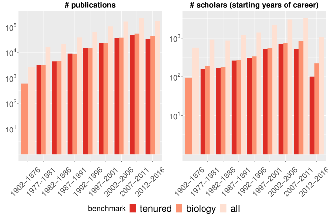
Figure 16: Exploratory Statistics of the Dataset. Left panel: number of papers published in a certain period; right panel: number of authors who start their careers in a certain period.

The dataset utilized for this study is from Google Scholar and includes active faculty members (assistant, associate, and full professors) in multiple disciplines from the top $10$ universities in the United States, which totals $14,358$ scholars. It includes the citation history through $2016$ for each publication from these scholars; they contributed to more than $800,000$ publications altogether, which received approximately $100$ million citations collectively. An exploratory description of the dataset can be found in the Supplemental Material (Figure 16 and Table 4).

The dataset was collected in the following way. Two assistants gathered the information about the organizational structure of each university, and from the web page of each department, we collected the information about the faculties. Then, for each faculty we utilized the author search in Google Scholar to identify the corresponding Google Scholar profile. The two independent assistants ensured that the collected data points were correct. When disagreement arose, they collaborated to resolve the differences.

The dataset allows us to study three benchmarks that are of practical interest: all publications and scholars, tenured professors, and the field of biology. We utilize the various benchmarks to demonstrate the generality and robustness of the study in this paper. The first benchmark contains all the publications and scholars in the dataset. The tenured professors are scholars who received their tenureships by $2016$. The biology benchmark consists of scholars whose area of interest on the Google Scholar page contains any of the following keywords: biology, genetic, neuroscience, or cell.

The dataset and the code to reproduce the results in this paper are available online at https://github.com/sentian/SciImpactRanking.

Framework for Calculating the Rank Percentile Indicator

Four fundamental elements of the rank percentile are entity, benchmark, evaluation metric, and age. The entity can be either a publication (P) or a scholar (S). The benchmark characterizes the reference set to which the entity is compared and is specified by the problem of interest. In a tenureship promotion example, the benchmark can comprise all cohorts in the same department, while in a research funding allocation example, the benchmark contains all the candidates in competition. The cohorts in the benchmark are evaluated utilizing a specified metric (m), such as the number of citations or the h-index [34], and the age $t$ specifies the time at which the evaluation is executed. For a publication, age $t$ represents the number of years since publication. For a scholar, age $t$ specifies the number of years since the beginning of the scholar’s academic career, which is represented by the scholar’s first publication.

With a specified benchmark, the rank percentile for publication $j$, denoted as P${}_{m}^{j}(t)$, is calculated in the following way.

1. Take a subset of publications in the benchmark that were published for more than $t$ years, and denote the size of the subset as $N$.

2. Evaluate these publications by their performance at age $t$. Utilize the evaluation metric to calculate the rank r${}_{m}^{j}(t)$ of publication $j$ against other publications. An average rank is assigned to r${}_{m}^{j}(t)$ if there exist other publications that have the same value of the metric.

3. The rank percentile is indicated by $\text{P}_{m}^{j}(t)=\left(\text{r}_{m}^{j}(t)-0.5\right)/N$.

With the compromise of $0.5/N$ in the final step, the median paper is assigned to the 50th percentile, and the tails of the citation distribution are treated symmetrically [35, 2]. The above framework can be easily adapted to compute the rank percentile indicators for scholar $i$, which is denoted as S${}_{m}^{i}(t)$.

The Rank Percentile Indicator for Scholars

For publication $j$, we utilize the number of citations (c) by age $t$ as the evaluation metric and denote the rank percentile indicator as P${}_{c}^{j}(t)$. We further utilize the publication indicators to construct the rank percentile for scholars. For scholar $i$, the performance is determined by the quantity and quality of the scholar’s publications, and each publication is evaluated via P${}_{c}^{j}(5)$, meaning the rank percentile for the paper in the 5th year since publication. We exclude publications with less than a 5-year history in the evaluation. The evaluation metric for scholar $i$ is determined by aggregating the performance of all $N(t)$ papers that the scholar publishes by age $t$, that is $\displaystyle\sum_{j=1}^{N(t)}\text{P}_{c}^{j}(5)$. We denote the resulting rank percentile indicator as S${}_{P5}^{i}(t)$, where P5 indicates the evaluation metric based on rank percentile indicator of publications in the 5th year since publication. In the discussion that follows, we utilize the simplified notations P_c and S_P5 to refer to the publication and scholar rank percentiles, respectively. The full notations are utilized in occasions when we refer to a specific entity or a specific age.

Figure 1 presents an example of S_P5 for a random scholar in our dataset in which the benchmark is tenured professors. The scholar’s career began in 2004, and our dataset tracks the citation information until 2016. The indicator S_P5 ranks the scholar in the top $45\%$ throughout the majority of their career. The figure indicates two other types of rank percentile indicators, S_c and S_h, which utilize the number of citations and h-index score, respectively, (the maximum number $h$ for which the scholar has $h$ publications, each with at least $h$ citations) as evaluation metrics for the scholar. We see that S_h largely agrees with S_P5, and S_c ranks the scholar lower than the other two indicators.

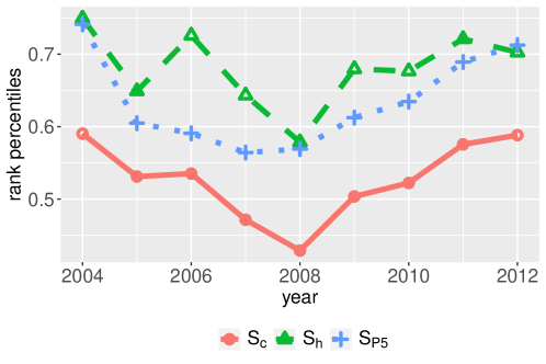
Figure 1: Rank Percentile Indicators for a Random Scholar in the Dataset. The benchmark is the tenured professors.

The indicator S_P5 improves some major drawbacks of S_c and S_h. First, it removes the seniority effect of publications. The evaluation metric for S${}_{c}^{i}(t)$ represents the citations that scholar $i$ receives by age $t$, which is the sum of citations for the scholar’s publications by $t$. Compared to newly published works, publications with longer histories are more likely to attract citations and therefore provide a greater contribution to formulating S_c. A similar argument can be made for S_h. However, S_P5 treats the publications equally and evaluates them based on their performances at the publications’ age of 5 years. Additionally, a scholar who publishes a considerable number of low-impact works or participates in only a small number of high-impact projects can have a high value of S_c, since the absolute number of citations can be unlimited and is significantly influenced by extreme values. However, the S_P5 and S_h of these scholars are not necessarily large, since these indicators limit the contribution of a single publication to be, at most, $1$ by definition of rank percentile and h-index score. Furthermore, compared to S_h, S_P5 penalizes scholars who are not truly innovative but carefully massage their h-index scores by publishing a number of papers that attract citation numbers that are barely sufficient to increase their h-index scores. If a paper is among the top $h$ papers, then the actual number of citations is irrelevant for the h-index and S_h, but it can still impact S_P5. Finally, S_P5 requires less data than S_c and S_h, since it only relies on the 5-year citation history of each publication. Hence, S_P5 is better suited to large-scale analysis.

We demonstrate the advantages of S_P5 by examining some extreme cases. We considered a benchmark that contains scholars in biology who started their careers in 1990, and we created three synthetic academic careers, adding them to the benchmark just for this experiment. Scholar A publishes a substantial number of publications throughout their career (more papers than $90\%$ of their cohorts in the benchmark), although each of the publications has little impact. Scholars B and C publish only one paper each at the beginning of their careers; B’s paper is astonishing, while C’s paper is average. Both scholars have an h-index equal to $1$ throughout their careers. Figure 2 illustrates the rank percentile indicators for these three artificial scholars. We see that flooding low-impact publications can increase S_c at the beginning of Scholar A’s career. Additionally, we see that a single high-impact work improves the value of S_c throughout Scholar B’s career; the author remains in the top $50\%$ at age $12$, as indicated by S_c. Both S_P5 and S_h better characterize the performances of these authors. Finally, S_h remains the same for Scholars B and C since they each have an h-index of $1$ throughout their careers. However, S_P5 considers that Scholar B’s publication has a greater impact and therefore ranks Scholar B higher than Scholar C.

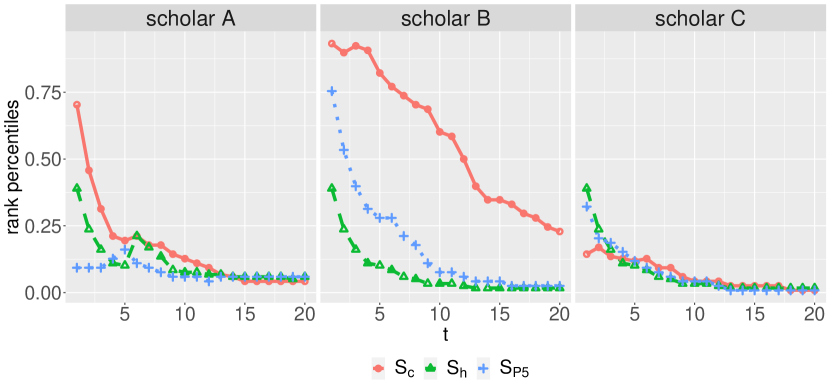
Figure 2: The Rank Percentile Indicators for Three Artificial Scholars. The benchmark contains scholars in biology who started their careers in $1990$.

With the exception of the above-mentioned discrepancies, we present in the Supplemental Material Section A that for the majority of scholars in our dataset, S_P5 largely agrees with S_c and S_h. Furthermore, we demonstrate the choice of utilizing the 5-year history of a publication. We considered utilizing a longer history (10 years) and found that (as evidenced in the Supplemental Material Section B) the differences between the resultant rank percentile indicator and S_P5 were not statistically significant. A similar conclusion can be obtained by utilizing summary statistics (mean, median, and max) of the rank percentile throughout the entire history of a publication instead of utilizing values at a fixed age, thus indicating the robustness of S_P5. As we will discuss in the following sections, the publication percentile P${}_{c}^{j}(t)$ is highly stable over $t$, and therefore P${}_{c}^{j}(5)$ is a reasonable indicator of the performance for the publication.

Additionally, we sum the rank percentiles for all the publications to obtain the evaluation metric for the scholar. The choice of the sum as the aggregation function considers both the quantity and the quality of the publications, which is in the same spirit of citation counts and h-index values. Another choice of the aggregation function can be the median. Unlike the sum, utilizing median publication impact minimizes the effect of quantity, and it can be favorable in situations like flooding low-impact publications. We provide a comprehensive comparison of the two aggregation functions and demonstrate the advantage of utilizing sum in the Supplemental Material Section C. We find that in most cases, utilizing sum and considering the quantity of publications provide more reasonable results. Even in the scenarios where median is more appropriate, we do not find utilizing sum to be undesirable. Furthermore, we observe that unlike utilizing sum, the scholar rank percentile based on median publication impact is not stationary, and hence it is no longer valid to compare scholars with different seniorities due to the presence of systematic bias. Last but not least, we notice a significantly higher predictive power of scholar rank percentile based on the sum of publication impacts.

The Stationarity of Rank Percentile Indicator

The rank percentile S_P5 allows us to compare a scholar with others in the benchmark at a specific age. In the example of the tenure promotion, we compared the 6-year performance of the candidate with the 6-year performance of the senior cohorts. The comparison is not valid if systematic bias exists in which exterior factors, such as the academic environment, result in a better or worse candidate performance than the internal factors, such as creativity and productivity.

Figure 3 portrays S_P5 at scholar age $5$, grouped by the starting year of academic careers, in which the benchmark is the tenured professors. We see that S_P5 does not exhibit an obvious upward or downward trend, which would indicate a systematic bias of the indicator that favors junior or senior scholars. The approximate stationarity over the starting year of careers provides empirical evidence for the validity of the rank percentile indicator.

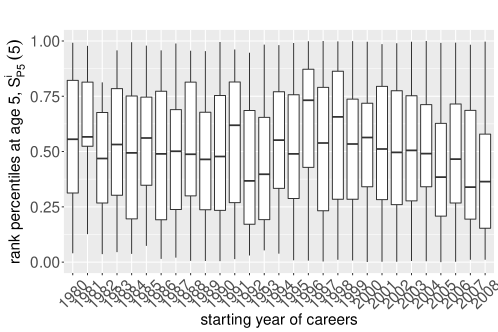
Figure 3: S${}_{P5}^{i}(5)$ Grouped by the Starting Years of Academic Careers. The benchmark is the tenured professors.

The Predictability of Rank Percentile Indicator

Citations have been proven to lack long-term predictive power [21]; consider the benchmark of biology as an example. Figure 4(a) illustrates that papers with the same number of citations by the 5th year since publication can have noticeably different citation paths and long-term effects. Additionally, exceptional and creative ideas typically require a lengthy period to be appreciated by the scientific community. The citation distribution over $30$ years since publication has been proven to have fat tails [21]. As presented in Figure 4(b), the correlation between short- (5-year) and long-term (30-year) citations disintegrates for the most highly-cited publications (the shaded rectangle). These problems can be largely avoided by utilizing rank percentile indicators, as evidenced in Figure 5. The considerable variation in the long-term effect of citations is restricted by utilizing rank percentiles. For publications with high impact, the correlation between short- (5-year) and long-term (30-year) effects persists when utilizing rank percentiles.

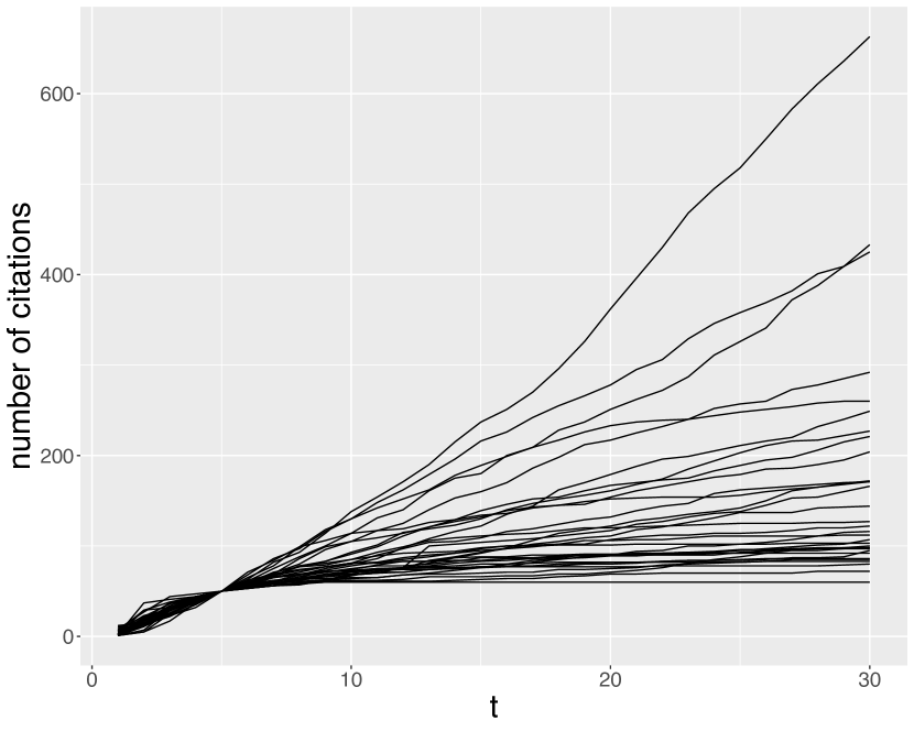
(a) Number of citations versus age

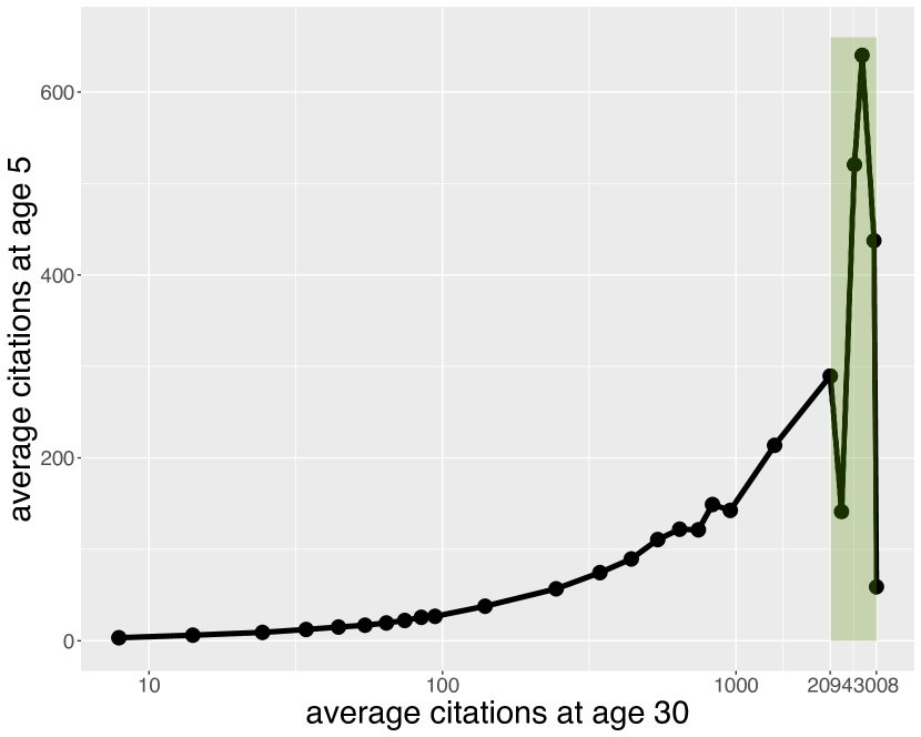
(b) Average citations at age $5$ versus those at age $30$

Figure 4: Predictability of Citations. The benchmark is the field of biology. Figure 4(a) portrays the cumulative citations for publications that have $50$ citations by the 5th year since publication. Figure 4(b) displays the average citations by age $5$ versus the average citations by age $30$. The averages are calculated over groups of publications, which are prespecified by dividing the range of citations by age $30$ into equal intervals on the log scale. Note that we do not claim the originality of the figures, which have been illustrated via a different dataset [21].

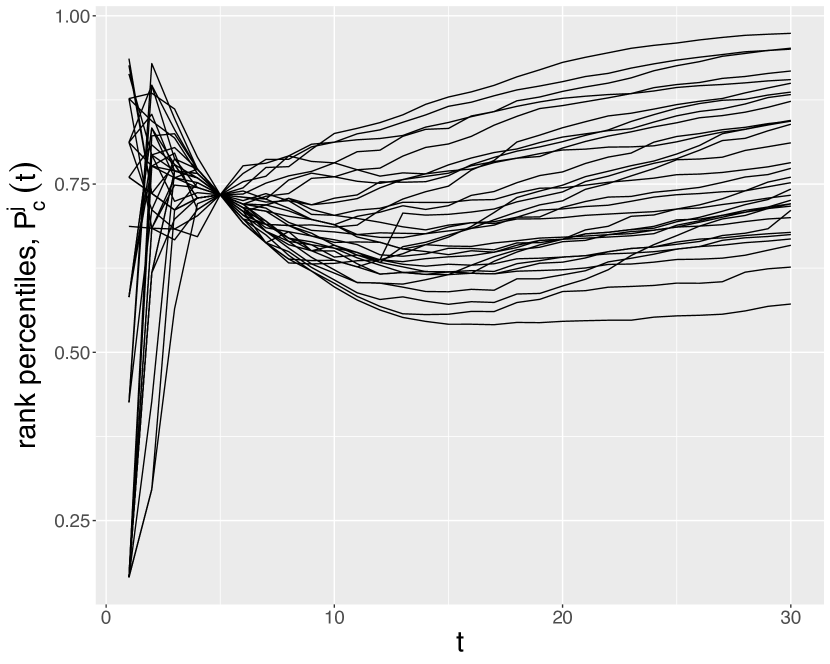
(a) Rank percentiles P_c versus age

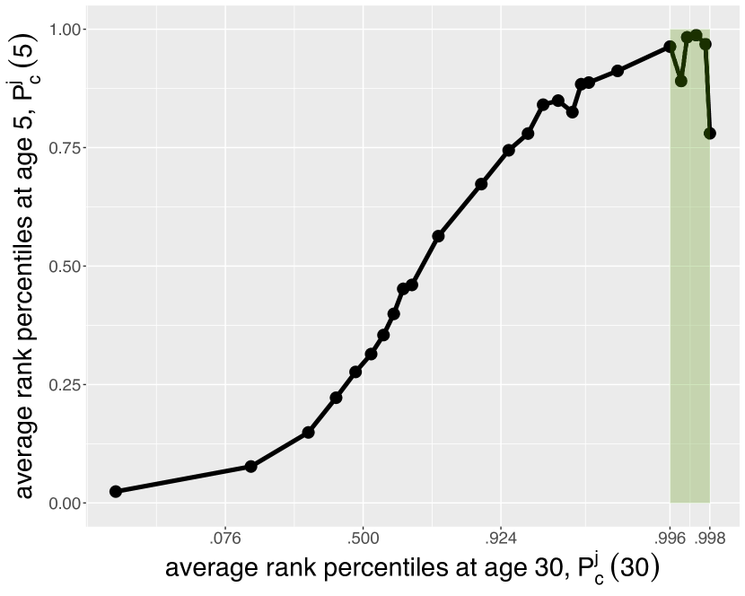
(b) Average P_c at age $5$ versus those at age $30$

Figure 5: Predictability of Rank Percentiles. Figure 5(a) demonstrates the rank percentiles for the publications considered in Figure 4(a). Figure 5(b) presents the average of P${}^{j}_{c}(5)$ versus the average of P${}^{j}_{c}(30)$ for the same groups of publications as in Figure 4(b).

We further characterize the predictability of rank percentile indicators. Figure 6(a) presents the Pearson correlation between rank percentiles at two ages, P${}_{c}^{j}(t_{1})$ and P${}_{c}^{j}(t_{2})$ where $t_{1}<t_{2}$. Overall, we noticed large correlations for both benchmarks. The correlation diminishes as the forecast horizon $(t_{2}-t_{1})$ increases, which simply reflects the difficulty of long-term forecasting. Additionally, the correlation increases as $t_{1}$ increases when the forecast horizon is fixed. This indicates that the performance of a senior publication is easier to predict, since the longer history removes more uncertainties regarding its performance. We further noticed a slightly higher predictive power when we restricted the benchmark to biology.

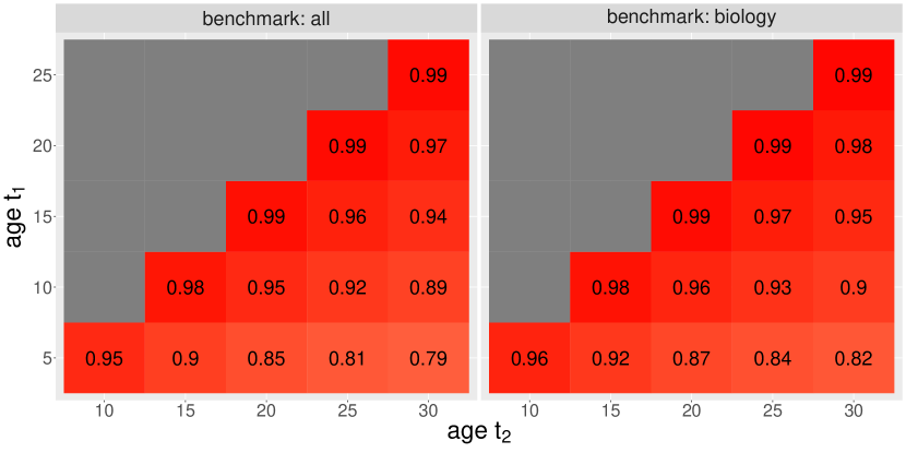
(a) Correlation between P${}_{c}^{j}(t_{1})$ and P${}_{c}^{j}(t_{2})$

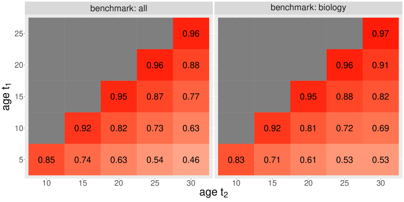
(b) Correlation between S${}_{P5}^{i}(t_{1})$ and S${}_{P5}^{i}(t_{2})$

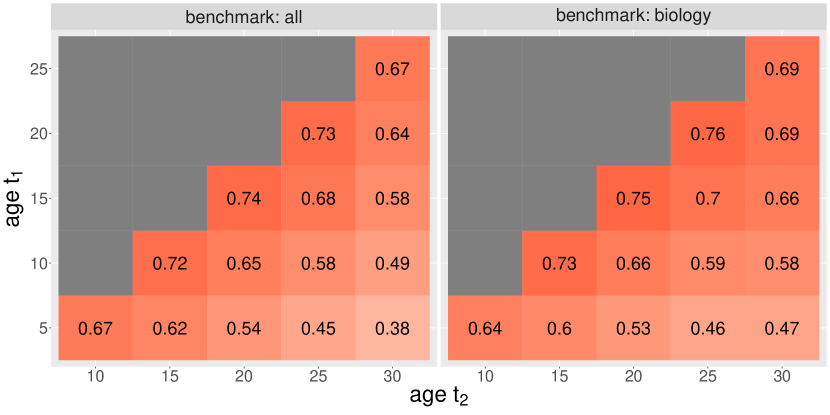
(c) Correlation between S${}_{P5}^{i}(t_{1})$ and S${}_{P5}^{i}(t_{2}|t_{1})$

Figure 6: Pearson Correlation between Rank Percentiles at Different Ages. The benchmark is either all or biology, and it is specified in each of the subfigures.

Figure 6(b) illustrates that the patterns discussed above generally hold for S_P5. However, the magnitude of correlations is smaller than those for publications, especially for long-term forecasts, because forecasting the future impact of future works is considerably more difficult than forecasting the future impact of existing works. The percentile S${}_{P5}^{i}(t_{2})$ is based on papers published before $t_{2}$, which can be divided into papers published before $(t_{1}-5)$, between $(t_{1}-5)$ and $t_{1}$, and between $t_{1}$ and $t_{2}$. Since we utilized P${}_{c}^{j}(5)$ (the publication rank percentile by 5 years since publication) to evaluate each publication, the performance of papers published before $(t_{1}-5)$ was represented by $t_{1}$. Predicting the performance of papers published between $(t_{1}-5)$ and $t_{1}$ is thus predicting the future impact of existing works, while predicting the performance of those published between $t_{1}$ and $t_{2}$ is predicting the future impact of future works. However, predicting the publication indicator P${}_{c}^{j}(t_{2})$ involves predicting only the future impact of publication $j$, which is a considerably easier task. Additionally, when the forecast horizon increases while $t_{1}$ is fixed, additional future works are involved in predicting S${}_{P5}^{i}(t_{2})$; therefore, we see that the correlation decreases more quickly than when we predict P${}_{c}^{j}(t_{2})$.

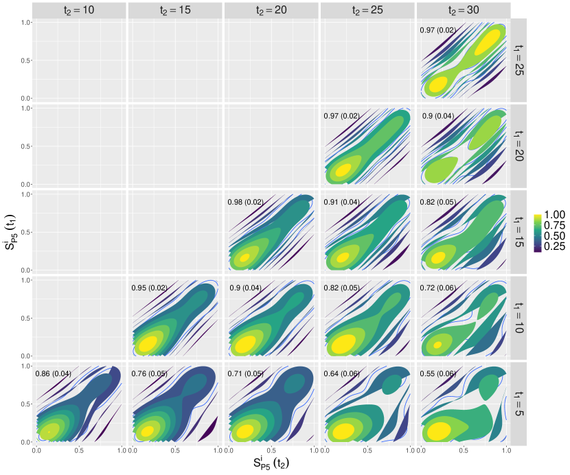
Figure 17: Kernel Density Estimation for the Scatter Points of S${}_{P5}^{i}(t_{1})$ and S${}_{P5}^{i}(t_{2})$. We fit a simple linear regression of S${}_{P5}^{i}(t_{2})$ on S${}_{P5}^{i}(t_{1})$. The estimated coefficient and the corresponding standard error (in the parentheses) are displayed in each plot. The benchmark contains all scholars in the dataset.

The strong linear relationship between P${}_{c}^{j}(t_{1})$ and P${}_{c}^{j}(t_{2})$ is further characterized in Figure 7, where we restricted, for a better visualization, the benchmark to be the publications in biology that were published in $1980$. The data are along the $45\degree$ line, and the linear regression coefficient of P${}_{c}^{j}(t_{2})$ on P${}_{c}^{j}(t_{1})$ is close to $1$ with small standard errors, thus indicating the high stability of P_c over time $t$. A similar figure for S_P5 is displayed in the Supplemental Material Figure 17, in which we find that S_P5 exhibits short-term stability.

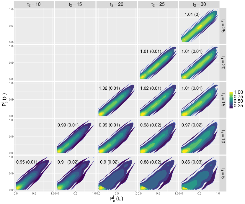
Figure 7: Kernel Density Estimation for the Scatter Points of P${}_{c}^{j}(t_{1})$ and P${}_{c}^{j}(t_{2})$. A simple linear regression of P${}_{c}^{j}(t_{2})$ on P${}_{c}^{j}(t_{1})$ is fitted. The estimated coefficient and the corresponding standard error (in parentheses) are displayed in each plot. The benchmark contains publications in biology that were published in $1980$.

Predicting S${}_{P5}^{i}(t_{2})$ can assist in decision-making for faculty positions or granting tenure, since the committee prefers to examine the cumulative scientific impact of the scholar. Committees assign research funding or allocate research resources regarding planned studies and potential future publications; consequently, the future impact of future works is often of interest. We utilized S${}_{P5}^{i}(t_{2}|t_{1})$ to denote the rank percentile indicator; this was calculated based on papers published between $t_{1}$ and $t_{2}$. Figure 6(c) illustrates the correlation between S${}_{P5}^{i}(t_{1})$ and S${}_{P5}^{i}(t_{2}|t_{1})$. The magnitudes of correlation are moderately high, indicating an approximately linear relationship, although the strength is less pronounced than it was in predicting the cumulative impact, that is, predicting S${}_{P5}^{i}(t_{2})$, which is consistent with our expectations.

A factor causing the difficulty in predicting the future impact of future works is the different stages of a scholar’s career. The first 5 years are typically when a scholar conducts their doctoral study and begins research under supervisions. The next 5 years of their academic career typically includes a postdoctoral study or an assistant professorship, in which the productivity and quality of works usually improve over those from the first 5 years, thus resulting in relatively low correlation (the value is $0.65$, according to Figure 6(c)) between S${}_{P5}^{i}(5)$ and S${}_{P5}^{i}(10|5)$. As the scholar earns seniority and produces a more consistent stream of publications, the discrepancy between different stages of their career becomes less discernible. For instance, the correlation increases to $0.7$, when $t_{1}=10$ and $t_{2}=15$.

Predictive Models

In this section, we formulate the prediction tasks as supervised learning problems, and we illustrate that the rank percentile indicators can be predicted via simple linear models. We consider the following fitting procedures; these models are ordered by increasing complexity:

• Baseline: simple linear regression model.

• Simple Markov model (sm).

• Penalized linear regression models, including the ridge [36], lasso [37], elastic net (enet) [38] and the Gamma lasso (gamlr) [39].

• Ensemble methods of regression trees, including the random forest (rf) [40] and extreme gradient boosting trees (xgbtree) [41].

• Neural networks (nnet).

Recall that the three prediction tasks discussed in the above section are predicting the future impact of publication percentile, the future impact of scholar percentile, and the future impact of scholar percentile based on futuer works, where the target variables are P${}_{c}^{j}(t_{2})$, S${}_{P5}^{i}(t_{2})$, and S${}_{P5}^{i}(t_{2}|t_{1})$, respectively. The baseline model fits a simple linear regression of the target variable on the autoregressive feature, such as P${}_{c}^{j}(t_{1})$ for predicting the publication impact. The simple Markov model further considers the change of the autoregressive feature in the past two ages, for instance P${}_{c}^{j}(t_{1})$-P${}_{c}^{j}(t_{1}-2)$, in addition to the autoregressive feature; furthermore, it fits a linear regression model.

Features and Model Fitting

For the remainder of the methods, we created an extensive list of features based on the citation histories. The features were characterized as either scholar- or publication-based features. For example, to predict the scholar indicator S${}_{P5}^{i}(t_{2})$, a scholar-based feature is the number of papers that scholar $i$ publishes by age $t_{1}$, and a publication-based feature is the average number of citations for these papers. We established $30$ features for predicting the publication indicator and $42$ features for predicting the scholar indicator, which can be found in the Supplemental Material Tables 2 and 3, respectively. Note that many of the features have been utilized when formulating the prediction task for number of citations and h-index scores [31, 29, 33].

The features were created utilizing the citation information available via $t_{1}$, and the dependent variable was specified at $t_{2}$. We considered five stages of a publication or a scholar: $t_{1}\in\{5,10,15,20,25\}$, and we forecasted through $30$ years of age: $t_{2}=t_{1}+1,\cdots,30$; this resulted in $75$ pairs of $(t_{1},t_{2})$ in total. Every model was trained $75$ times, once for each pair of $(t_{1},t_{2})$.

The rank percentiles were calculated utilizing all the publications and scholars in the dataset. We then restricted data for the prediction task to maintain the same set of publications and scholars for the entire forecast horizon (up to 30 years). To predict the publication impact, we employed a subset of data by including papers with more than $30$ years of age, which corresponds to papers published before 1987, since the most recent year considered in the dataset is 2016; this resulted in $36,372$ papers. Similarly, for the scholar impact prediction task, we utilized scholars who started their careers before 1987; this resulted in $1,457$ scholars.

We also noted (in the Supplemental Material Section D) that both S_P5 and P_c were non-stationary time series, as evidenced by the Dicky-Fuller test [53] and the KPSS test [54]. The differenced series were stationary (also presented in the Supplemental Material) and were utilized as the response variables: $\Delta\text{P}_{c}^{j}(t_{2})=\text{P}_{c}^{j}(t_{2})-\text{P}_{c}^{j}(t_{1})$, $\Delta\text{S}_{P5}^{i}(t_{2})=\text{S}_{P5}^{i}(t_{2})-\text{S}_{P5}^{i}(t_{1})$, and $\Delta\text{S}_{P5}^{i}(t_{2}|t_{1})=\text{S}_{P5}^{i}(t_{2}|t_{1})-\text{S}_{P5}^{i}(t_{1})$. Note that the stationarity discussed here characterizes the property of S_P5 and P_c as time series. It is different from the stationarity as discussed in Figure 3, in which we fixed $t=10$ and examined the stationarity of S${}_{P5}(10)$ over the starting year of the scholars’ careers.

The machine learning methods were trained in R [44] utilizing the package mlr [45], which provides a pipeline of training, validating, and testing for the model. The lasso, ridge, elastic net, random forest, and xgbtree modles are built into the package. The Gamma lasso and neural network were trained utilizing R packages gamlr [39] and keras [46], respectively.

The machine learning methods require hyperparameter tuning, which involves deciding the search space of parameters and evaluating the sets of parameters utilizing the validation data. The hyperparameters for each machine learning model considered in this paper are presented in the Supplemental Material Table 1. Each hyperparameter has a grid of predefined values, and the search space is the combination of all parameters. The parameter space can be substantial for methods such as xgbtree and nnet, which utilize extensive lists of tunable parameters. For these methods, we applied Bayesian optimization, which searches over the parameter space based on the performance gain. The optimal choice of hyperparameters is that which minimizes the validation error, where a holdout validation set was utilized for xgbtree and nnet, and 10-fold cross-validation was employed for the other methods.

Performance of the predictive models

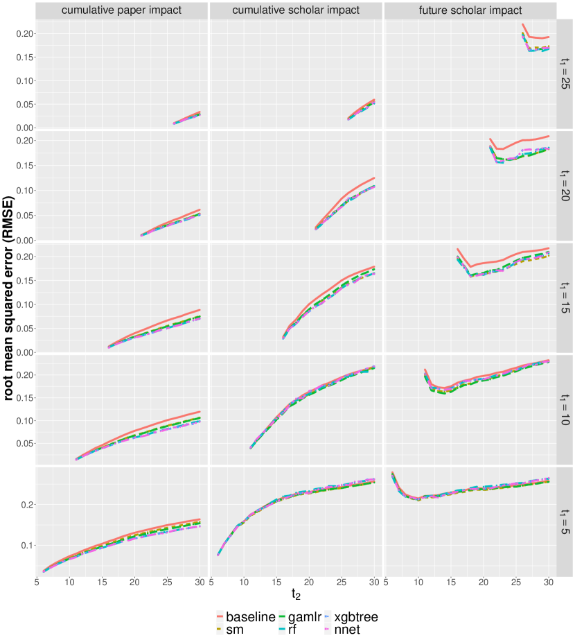
Figure 18: RMSE for the Predictive Models.

The data were randomly split into the training and test set at a 9:1 ratio. The accuracy of prediction on the holdout test set in terms of testing $R^{2}$ is presented in Figure 8. We see that the simple linear regression model predicted the cumulative impacts well, i.e. P${}_{c}^{j}(t_{2})$ and S${}_{P5}^{i}(t_{2})$, and the usage of a large number of features and complex machine learning models offered little improvement. Predicting the future impact of scholars, S${}_{P5}^{i}(t_{2}|t_{1})$, is considerably more difficult. The simple linear regression model provided reasonable predictions, but the performance was not as satisfactory as other methods, especially when $t_{1}$ was large. By adding the difference presented in $\text{S}_{P5}^{i}(t_{1})-\text{S}_{P5}^{i}(t_{1}-2)$ as an extra feature, the simple Markov model achieved similar performance compared to the complex machine learning models that rely on extensive lists of features and exhibit non-linear relationships. The conclusion is robust against the choice of error measure, and we present the results utilizing the root mean squared error, root median squared error, and mean absolute error in the Supplemental Material (Figure 18, 19, and 20, respectively).

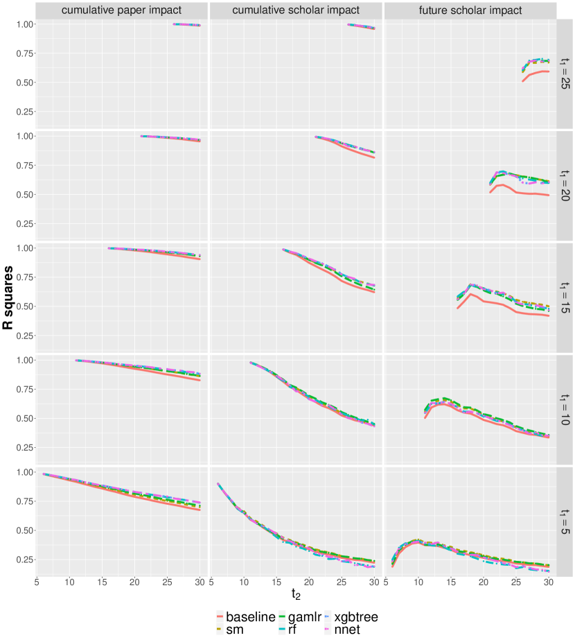
Figure 8: Testing $R^{2}$ for the Predictive Models. The target variables, from left to right panel, are P${}_{c}^{j}(t_{2})$, S${}_{P5}^{i}(t_{2})$, and S${}_{P5}^{i}(t_{2}|t_{1})$, respectively. The lasso, ridge, and elastic net are outperformed by the Gamma lasso, and hence are ignored for a better visualization.

The overall patterns in Figure 8 matches those in Figure 6. To predict the cumulative impact, we observe that the overall $R^{2}$ becomes larger as $t_{1}$ increases and the $R^{2}$ decreases as the forecast horizon increases. An interesting pattern that we did not observe previously (since the smallest forecast horizon in Figure 6 was $5$ years) is that for predicting the future scholar impact, the $R^{2}$ curves exhibit non-monotonic shapes. For instance, when $t_{1}=5$, the $R^{2}$ increases from approximately $0.25$ ($t_{2}=6$) to $0.5$ ($t_{2}=10$) before decreasing. A scholar’s first 5-year performance is not necessarily a quality indicator for the 6th-year performance, potentially due to external factors, such as the processing time of journals, which can be anywhere from months to years depending on the culture, quality of the venue, field, and availability of referees. Hence, a promising scholar may experience a publication drought in the 6th year simply because the submitted papers take longer than usual to be reviewed; this causes S${}_{P5}^{i}(5)$ to be a poor indicator for S${}_{P5}^{i}(6|5)$. The effect of the external factors diminishes as we allow a longer horizon ($t_{2}-t_{1}$) for the evaluation, and therefore we notice an increase of $R^{2}$ when $t_{2}$ becomes $10$. As $t_{2}$ further increases, the difficulty of long-term forecasting enters, and the $R^{2}$ decreases.

Conclusion

Rank percentile has been demonstrated to be a better indicator of the performance for a publication or a scholar compared to other types of field- and time- normalized indicators. Rank percentile is highly interpretable, and it provides flexibility in the choice of benchmark and evaluation metrics. In this paper, we proposed a novel rank percentile for scholars that has clear advantages over the traditional rank percentile, which is based on citation counts or h-index values. Furthermore, we focused on the time factor and studied the predictability of rank percentile. We illustrated that the rank percentile has significant predictive power. In particular, the publication percentile is highly stable over time, and the scholar percentile exhibits short-term stability. Although complex machine learning models that utilize an extensive list of features can provide slightly better predictive performance, the linear regression model with merely the autoregressive and difference features provides considerable prediction accuracy; thus indicating the ease of predicting rank percentile. In practice, the highly predictable rank percentile can be utilized in combination with other metrics to picture the trajectory of a scholar or a publication and assist in academic decision making.

Limitation and Future Work

A key limitation of our study is the survivorship bias built into the dataset of scholars. The dataset consisted of scholars who were either assistant, associate, or full professors in the top U.S. institutions through $2016$, and hence, we were more likely to include scholars who have been successful over the long term. We do not have a control set of researchers who have left the academic track by, for example, moving to the industry or failing to obtain tenureship. In future work, we should analyze which of the lower-performing junior scholars earn tenure and continue their academic career as well as which of them leave the academic track. We have some evidence that our metrics can be utilized for such predictions, which in turn can be utilized to control for the survivorship bias in our dataset.

Another limitation is the lack of thorough field-specific analyses. The rank percentile has been demonstrated to be problematic as a field-normalized indicator when papers cover multiple disciplines and when papers have multiple authors [13]. A solution is to fractionally assign the papers to the disciplines or authors [47, 48]. Additionally, the rank percentile lacks cross-field and cross-scale stability [49]. In our experiments, however, we did not notice a systematic difference between the field of biology and fields that encompass multiple disciplines. This does not mean that there are no field differences; it simply means that our dataset and analysis did not have the necessary power to clearly reveal the field-specific differences.

We also acknowledge that the systematic bias (e.g. the time, cohort, and environment effect) can exist in other datasets or benchmarks, even though it does not present in our study. A potential solution to eliminate the bias is to restrict the benchmark, for instance only including cohorts with the same seniority or in the same field. A thorough method to remove the systematic bias is an interesting future work.

The bibliographic metrics considered in this paper that are the citation counts and h-index values, treat citations equally and do not distinguish between citations from highly regarded journals and citations from workshop panels. PageRank index [50, 51, 52] utilizes the citation network and evaluates a publication by assigning different weights to its citations. In future work, it would be interesting to compare the PageRank-based percentile with the percentiles studied in this paper.

Appendix A Comparison of Various types of Scholar Percentiles

We consider the benchmark being the field of biology. In order to study the agreement of various indicators, for each indicator, we classify the scholars into four classes, class $1$: $0\leq\text{S}_{m}^{i}(t)<0.25$, class $2$: $0.25\leq\text{S}_{m}^{i}(t)<0.5$, class $3$: $0.5\leq\text{S}_{m}^{i}(t)<0.75$ and class $4$: $0.75\leq\text{S}_{m}^{i}(t)\leq 1$. An agreement is when two (or three) different indicators belong to the same class. The overall agreement for all three indicators, S_P5, S_c, and S_h, is $51\%$ at age $5$ and $68\%$ at age $30$; that is, for about half of the scholars the three indicators agree with each other at age $5$, while that number becomes around two third at age $30$. Figure 9 displays pairwise agreement of the three indicators. We see that the agreement increases with the age. Furthermore, S_P5 has large agreement with both S_c and S_h, which are $69\%$ and $67\%$, respectively, at age $5$, and $71\%$ and $81\%$, respectively, at age $30$.

Figure 10 shows the correlation between S${}_{c}^{i}(t_{1})$ and S${}_{c}^{i}(t_{2})$, and the correlation between S${}_{h}^{i}(t_{1})$ and S${}_{h}^{i}(t_{2})$. The magnitudes of correlations are similar to those for S_P5 as shown in Figure 6(b).

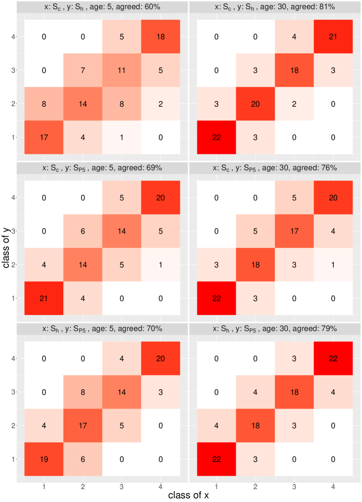
Figure 9: The Agreement of Rank Percentile Indicators for Scholars. Rank percentile indicators are classified into four groups, that are class $1$: $0\leq\text{S}_{m}^{i}(t)<0.25$, class $2$: $0.25\leq\text{S}_{m}^{i}(t)<0.5$, class $3$: $0.5\leq\text{S}_{m}^{i}(t)<0.75$ and class $4$: $0.75\leq\text{S}_{m}^{i}(t)\leq 1$. The agreement of classes (sum of the anti-diagonal elements) is displayed in the title of each panel. The benchmark is biology. The agreement for all three indicators is $51\%$ at age $5$ and is $68\%$ at age $30$.

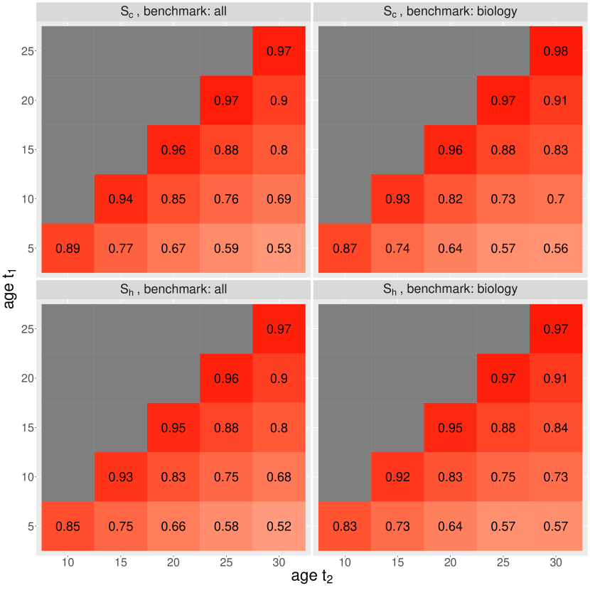
Figure 10: Pearson Correlation between Rank Percentiles at Different Ages. This supplements the results in Figure 6(b).

Appendix B Evaluation of Publications in Formulating Scholar Percentile

Recall that S${}_{P5}^{i}(t)$ is calculated based on an aggregation of the performances of publications that scholar $i$ publishes by age $t$. Denote $\text{m}_{P5}^{i}(t)$ as the evaluation metric of scholar $i$ at age $t$ based on $\text{P}_{c}^{j}(5)$, that is $\text{m}_{P5}^{i}(t)=\sum_{j=1}^{N(t)}\text{P}_{c}^{j}(5)$, where $N(t)$ is the total number of publications of scholar $i$ by age $t$. We illustrated in the paper that P${}_{c}^{j}(t)$ exhibits high stability over $t$, and hence P${}_{c}^{j}(5)$ can be applied to represent the performance of the publication.

We further demonstrate the robustness of S_P5 by considering a longer citation history for each publication. Figure 11 illustrates that m${}_{P5}^{i}(t)$ is highly correlated with m${}_{P10}^{i}(t)$ at age $t=1,\cdots,30$, where m${}_{P10}^{i}(t)=\sum_{j=1}^{N(t)}\text{P}_{c}^{j}(10)$. We also consider utilizing the maximum, mean and median values of P${}_{c}^{j}(t)$, for instance m${}_{Pmax}^{i}(t)=\sum_{j=1}^{N(t)}\max_{t^{\prime}}\text{P}_{c}^{j}(t^{\prime})$. We see from Figure 11 that these metrics also exhibit high correlations with m_P5. Furthermore, we perform a Wilcoxon paired signed-rank test to compare the differences between S${}_{P5}^{i}(t)$ and S${}_{P10}^{i}(t)$ at each age $t=1,\cdots,30$, and the p-values are close to $1$; indicating that the differences are not statistically significant. Similar conclusions can be drawn for other indicators (S_Pmax, S_Pmean, and S_Pmedian) being considered.

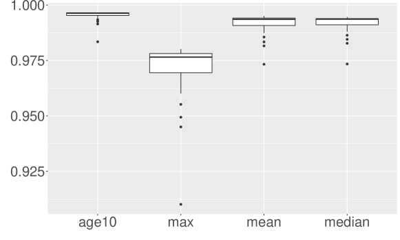
Figure 11: Correlation between m_P5 and Other Choices of Evaluation Metric. The benchmark contains all scholars in the dataset. Age $10$, max, mean and median correspond to m_P10, m_Pmax, m_Pmean and m_Pmedian, respectively. The correlation is calculated at each age $t=1,\cdots,30$.

Appendix C Aggregation Function in Formulating Scholar Percentile

We use sum as the aggregation function in calculating the scholar percentile, that is $\text{m}_{P5}^{i}(t)=\sum_{j=1}^{N(t)}\text{P}_{c}^{j}(5)$. Another favorable choice is median, i.e. $\text{m}_{P5}^{i}(t)=\text{median}_{j}\text{P}_{c}^{j}(5)$. We provide empirical evidence of the advantage of utilizing sum over median. We use S_P5.sum and S_P5.median to denote the rank percentiles formulated based on the sum and median publication impacts, respectively.

The first reason that we prefer sum over median is that S_P5.sum is stationary while S_P5.median is not. Stationarity provides the foundation for the study in this manuscript. Without stationarity, the comparison of the 6-year performance of the candidate and the 6-year performance of the senior cohorts in the example of the tenure promotion will not be valid, due to the presence of systematic bias. We see in Figure 3 that S_P5.sum is approximately stationary. However, as indicated in Figure 12, S_P5.median exhibits a clear upward trend and favors the junior scholars.

The second reason is that using sum takes both the quality and quantity of publications into account. This is in the same spirit as citation counts and h-index, the two most commonly used bibliographic metrics. However, using median largely minimizes the effect of quantity. A scholar who participates in only a small number of high-impact projects, e.g. PhD student, can rank higher than a scholar who consistently produces impactful publications. In Figure 2, the artificial scholar B only publishes one highly regarded article throughout the entire career. We see that S_P5.sum ranks the scholar in the top $25\%$, and the rank dies down to be in the bottom $10\%$ at age 10. The same pattern can be observed for S_c and S_h (rank percentiles based on citations and h-index, respectively). A corresponding plot using S_P5.median is displayed in Figure 13, where the scholar has a constant rank close to 1 throughout the career. It is not unreasonable to question that the scholar is still on top 20 years after the single publication, and therefore, the sum is preferred in this example.

Another example in Figure 2 is the artificial scholar A who publishes a substantial number of low-impact publications throughout the career. We observe that S_P5.sum starts from around $10\%$ and gradually dies down to around $5\%$ at age 10. This indicates that flooding low-impact publications may slightly works at the beginning of the career, and it is not a good strategy in the long run. The pattern arguably makes more sense than the constant S_P5.median as displayed in Figure 13. Furthermore, S_P5.sum is almost always below S_c and S_h; indicating that it is more robust against flooding low-impact works.

The last and arguably most important reason that we prefer sum is that the predictive power of S_P5.sum is much higher than S_P5.median. If we compare Figure 6(b) with 14(a), the overall correlation drops by around $5\%$. The correlation drops by about $50\%$ for predicting the future impact of future works, as revealed in Figure 6(c) and 14(b).

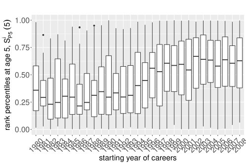
Figure 12: S${}_{P5}^{i}(5)$ Grouped by the Starting Years of Academic Careers. The benchmark is the tenured professors. The aggregation function in formulating S${}_{P5}^{i}(5)$ is median.

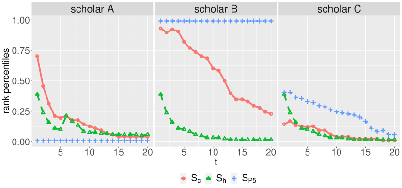
Figure 13: The Rank Percentile Indicators for Three Artificial Scholars. The benchmark contains scholars in biology who started their careers in $1990$. The aggregation function in formulating S${}_{P5}^{i}(5)$ is median.

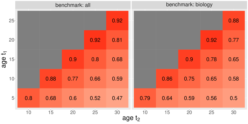
(a) Correlation between S${}_{P5}^{i}(t_{1})$ and S${}_{P5}^{i}(t_{2})$

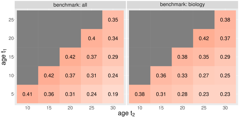
(b) Correlation between S${}_{P5}^{i}(t_{1})$ and S${}_{P5}^{i}(t_{2}|t_{1})$

Figure 14: Pearson Correlation between Rank Percentiles at Different Ages. The benchmark is either all or biology, and it is specified in each of the subfigures. The aggregation function in formulating S${}_{P5}^{i}(5)$ is median.

Appendix D Stationarity Test for Rank Percentiles and Their Differenced Series

Two commonly used statistical tests for stationarity are the Dicky-Fuller test [53] and KPSS test [54]. These two tests formulate the hypothesis testing problems differently. Dicky-Fuller test assumes a unit root presented in the series. A unit root means that the series is $I(1)$, i.e. integrated order $1$ and the first differenced series is stationary. The more negative the test statistic is, the stronger the rejection of the null. On the other hand, KPSS test assumes the null as the series being stationary, i.e. $I(0)$. KPSS test is slightly more general since it allows testing a series being non-stationary but does not present a unit root. The more positive the test statistic is, the stronger the rejection of the null. Both tests include the drift in the test equations but exclude the trend, since we do not observe significant trends in the series.

The test statistics are shown in Figure 15. The dashed lines indicate the critical values at $5\%$ level. KPSS test indicates that P_c and S_P5 are non-stationary series, and we do not have enough evidence to reject them being $I(1)$ according to the Dicky-Fuller test. Furthermore, the differenced series are stationary based on both tests.

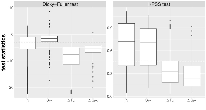
Figure 15: Statistical Tests for the Stationarity of Rank Percentile Series. Both tests are applied on every individual series, and the test statistics are presented. The $5\%$ critical value for each test is illustrated by the dashed horizontal line. Both tests suggest that publication indicator P_c and scholar indicator S_P5 are non-stationary, while their differenced series are stationary.

Method	Tuning parameters
Lasso	Penalty strength parameter
Ridge	Penalty strength parameter
Elastic net	Penalty strength parameter
	Penalty gap parameter
Gamma lasso	Penalty strength parameter
	Convexity parameter
Random forest	Number of trees to grow
	Number of variables used at each split
	Minimum number of observations in a node
xgbtree	Maximum number of iterations
	Learning rate
	Regularization parameter
	Maximum depth of the tree
	Minimum number of observations in each child leaf
	Number of observations supplied to a tree
	Number of features supplied to a tree
	Regularization parameter for ridge penalty
	Regularization parameter for LASSO penalty
Deep neural network	Number of layers
	Learning rate
	Number of hidden units at each layer
	Dropout rate
	Regularization parameter

Table 1: Hyperparameter(s) of the Machine Learning Models.

Feature	Description
pub_cit_cumulative	total citations of publication $j$
pub_cit_yearly	yearly citations of publication $j$ received in $t_{1}$
pub_cit_peryear	average citations of publication $j$ over age
pub_rp_cumulative	rank percentile indicator calculated based on total citations, i.e. P${}_{c}^{j}(t_{1})$
pub_rp_yearly	rank percentile indicator calculated based on yearly citations at $t_{1}$
aut_cit_cumulative	total citations of author $i$
aut_cit_yearly	yearly citations of author $i$ at $t_{1}$
aut_npub_cumulative	total number of publications of author $i$
aut_npub_yearly	yearly number of publications of author $i$ at $t_{1}$
aut_cit_perpaper	average citations per paper for author $i$
aut_h_index	h-index of author $i$
aut_g_index	g-index of author $i$
aut_maxcit_pub	largest citation that a single paper of author $i$ has received
aut_rprp5_cumulative	rank percentile calculated based on all papers, i.e. S${}_{P5}^{i}(t_{1})$
aut_rprp5_yearly	rank percentile calculated based on just papers written at $t_{1}$
_delta	the difference over the last two ages for each of the above features

Table 2: Features for Predicting the Publication Impact.

Feature	Description
aut_cit_cumulative	total citations of author $i$
aut_cit_yearly	yearly citations of author $i$ at age $t_{1}$
aut_npub_cumulative	number of publications of author $i$
aut_npub_yearly	yearly number of publications of author $i$ at age $t_{1}$
aut_h_index	h-index of author $i$
aut_g_index	g-index of author $i$
aut_cit_peryear	average citations per age of author $i$
aut_rprp5_cumulative	rank percentile calculated using all publications, i.e. S${}_{P5}^{i}(t_{1})$
aut_rprp5_yearly	rank percentile calculated using just publications written in age $t_{1}$
pub_cit_cumulative_{min,mean,max}	citations received by each of the publications
pub_cit_yearly_{min,mean,max}	citations received by each of the publications written at age $t_{1}$
pub_rp_cumulative_{min,mean,max}	publication rank percentiles calculated based on total citations
pub_rp_yearly_{min,mean,max}	publication rank percentiles calculated based on citations at age $t_{1}$
_delta	the difference over the last two ages for each of the above features

Table 3: Features for Predicting the Scholar Impact.

Appendix E Other tables and figures

benchmark	all	biology	tenured
# publications	801239	194713	176404
# scholars	14358	3410	2706
# citations per publication by age 5	45	56	49
# citations per scholar by age 5	172	209	332

Table 4: Summary statistics of the dataset.

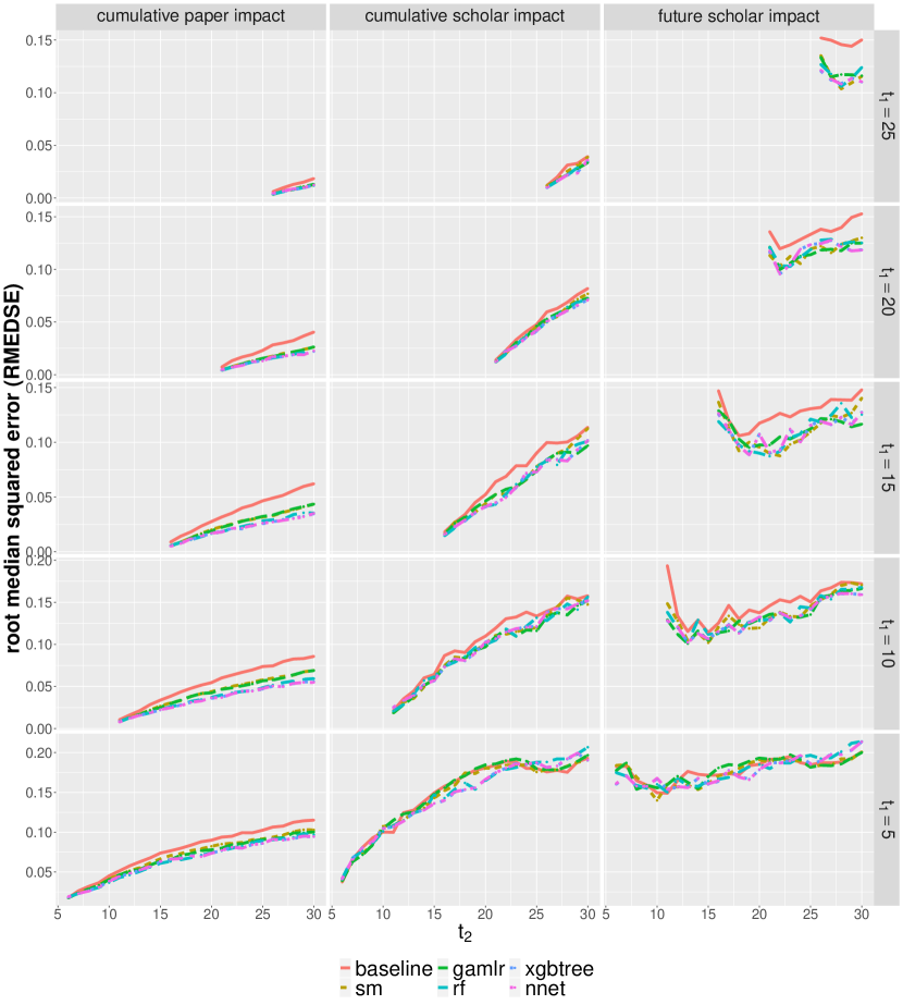
Figure 19: RMESE for the Predictive Models.

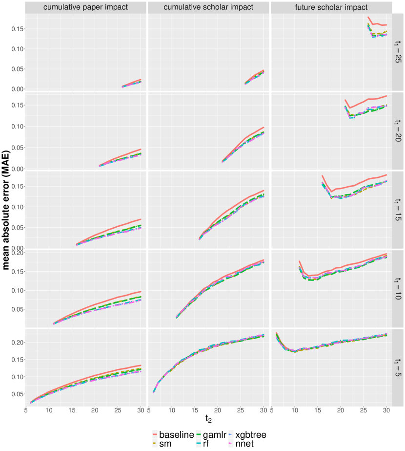
Figure 20: MAE for the Predictive Models.

References

- [1] András Schubert and Tibor Braun “Relative indicators and relational charts for comparative assessment of publication output and citation impact” In Scientometrics 9.5-6 Springer, 1986, pp. 281–291
- [2] Lutz Bornmann, Loet Leydesdorff and Rüdiger Mutz “The use of percentiles and percentile rank classes in the analysis of bibliometric data: Opportunities and limits” In Journal of Informetrics 7.1 Elsevier, 2013, pp. 158–165
- [3] Lutz Bornmann and Werner Marx “Methods for the generation of normalized citation impact scores in bibliometrics: Which method best reflects the judgements of experts?” In Journal of Informetrics 9.2 Elsevier, 2015, pp. 408–418
- [4] John Mingers and Loet Leydesdorff “A review of theory and practice in scientometrics” In European Journal of Operational Research 246.1 Elsevier, 2015, pp. 1–19
- [5] Lutz Bornmann, Alexander Tekles and Loet Leydesdorff “How well does I3 perform for impact measurement compared to other bibliometric indicators? The convergent validity of several (field-normalized) indicators” In Scientometrics 119.2 Springer, 2019, pp. 1187–1205
- [6] Ludo Waltman and Nees Jan Eck “Field normalization of scientometric indicators” In Springer handbook of science and technology indicators Springer, 2019, pp. 281–300
- [7] Diana Hicks et al. “Bibliometrics: the Leiden Manifesto for research metrics” In Nature 520.7548, 2015, pp. 429–431
- [8] Lutz Bornmann “How are excellent (highly cited) papers defined in bibliometrics? A quantitative analysis of the literature” In Research Evaluation 23.2 Oxford University Press, 2014, pp. 166–173
- [9] Lutz Bornmann and Werner Marx “Distributions instead of single numbers: Percentiles and beam plots for the assessment of single researchers” In Journal of the Association for Information Science and Technology 65.1 Wiley Online Library, 2014, pp. 206–208
- [10] Lutz Bornmann and Werner Marx “How to evaluate individual researchers working in the natural and life sciences meaningfully? A proposal of methods based on percentiles of citations” In Scientometrics 98.1 Springer, 2014, pp. 487–509
- [11] Richard Williams and Lutz Bornmann “The substantive and practical significance of citation impact differences between institutions: Guidelines for the analysis of percentiles using effect sizes and confidence intervals” In Measuring Scholarly Impact Springer, 2014, pp. 259–281
- [12] Lutz Bornmann and Robin Haunschild “Plots for visualizing paper impact and journal impact of single researchers in a single graph” In Scientometrics 115.1 Springer, 2018, pp. 385–394
- [13] Lutz Bornmann and Richard Williams “An evaluation of percentile measures of citation impact, and a proposal for making them better” In Scientometrics 124 Springer, 2020, pp. 1457–1478
- [14] Derek de Solla Price “A general theory of bibliometric and other cumulative advantage processes” In Journal of the American Society for Information Science 27.5 Wiley Online Library, 1976, pp. 292–306
- [15] Albert-László Barabási and Réka Albert “Emergence of scaling in random networks” In Science 286.5439 American Association for the Advancement of Science, 1999, pp. 509–512
- [16] George J Peterson, Steve Pressé and Ken A Dill “Nonuniversal power law scaling in the probability distribution of scientific citations” In Proceedings of the National Academy of Sciences 107.37 National Acad Sciences, 2010, pp. 16023–16027
- [17] Filippo Radicchi, Santo Fortunato and Claudio Castellano “Universality of citation distributions: Toward an objective measure of scientific impact” In Proceedings of the National Academy of Sciences 105.45 National Acad Sciences, 2008, pp. 17268–17272
- [18] Réka Albert and Albert-László Barabási “Statistical mechanics of complex networks” In Reviews of Modern Physics 74.1 APS, 2002, pp. 47
- [19] Kamalika Basu Hajra and Parongama Sen “Modelling aging characteristics in citation networks” In Physica A: Statistical Mechanics and its Applications 368.2 Elsevier, 2006, pp. 575–582
- [20] Sergey N Dorogovtsev and José Fernando F Mendes “Evolution of networks with aging of sites” In Physical Review E 62.2 APS, 2000, pp. 1842
- [21] Dashun Wang, Chaoming Song and Albert-László Barabási “Quantifying long-term scientific impact” In Science 342.6154 American Association for the Advancement of Science, 2013, pp. 127–132
- [22] J Wang, Y Mei and D Hicks “Science communication. Comment on “Quantifying long-term scientific impact".” In Science 345.6193, 2014, pp. 149–149
- [23] Dashun Wang, Chaoming Song, Hua-Wei Shen and Albert-László Barabási “Response to Comment on “Quantifying long-term scientific impact"” In Science 345.6193 American Association for the Advancement of Science, 2014, pp. 149–149
- [24] Lawrence D Fu and Constantin Aliferis “Models for predicting and explaining citation count of biomedical articles” In AMIA Annual symposium proceedings 2008, 2008, pp. 222 American Medical Informatics Association
- [25] Cynthia Lokker et al. “Prediction of citation counts for clinical articles at two years using data available within three weeks of publication: retrospective cohort study” In BMJ 336.7645 British Medical Journal Publishing Group, 2008, pp. 655–657
- [26] Alfonso Ibáñez, Pedro Larrañaga and Concha Bielza “Predicting citation count of Bioinformatics papers within four years of publication” In Bioinformatics 25.24 Oxford University Press, 2009, pp. 3303–3309
- [27] Amin Mazloumian “Predicting scholars’ scientific impact” In PLoS One 7.11 Public Library of Science, 2012, pp. e49246
- [28] David I Stern “High-ranked social science journal articles can be identified from early citation information” In PLoS One 9.11 Public Library of Science, 2014, pp. e112520
- [29] Luca Weihs and Oren Etzioni “Learning to predict citation-based impact measures” In Proceedings of the 17th ACM/IEEE Joint Conference on Digital Libraries, 2017, pp. 49–58 IEEE Press
- [30] Jorge E Hirsch “Does the h index have predictive power?” In Proceedings of the National Academy of Sciences 104.49 National Acad Sciences, 2007, pp. 19193–19198
- [31] Daniel E Acuna, Stefano Allesina and Konrad P Kording “Future impact: Predicting scientific success” In Nature 489.7415 Nature Publishing Group, 2012, pp. 201
- [32] Orion Penner et al. “On the predictability of future impact in science” In Scientific Reports 3 Nature Publishing Group, 2013, pp. 3052
- [33] James W Weis and Joseph M Jacobson “Learning on knowledge graph dynamics provides an early warning of impactful research” In Nature Biotechnology Nature Publishing Group, 2021, pp. 1–8
- [34] Jorge E Hirsch “An index to quantify an individual’s scientific research output” In Proceedings of the National Academy of Sciences 102.46 National Acad Sciences, 2005, pp. 16569–16572
- [35] Allen Hazen “Storage to be provided in impounding municipal water supply” In Transactions of the American Society of Civil Engineers 77.1 American Society of Civil Engineers, 1914, pp. 1539–1640
- [36] Arthur E Hoerl and Robert W Kennard “Ridge regression: Biased estimation for nonorthogonal problems” In Technometrics 12.1 Taylor & Francis Group, 1970, pp. 55–67
- [37] Robert Tibshirani “Regression shrinkage and selection via the lasso” In Journal of the Royal Statistical Society. Series B (Methodological) JSTOR, 1996, pp. 267–288
- [38] Hui Zou and Trevor Hastie “Regularization and variable selection via the elastic net” In Journal of the Royal Statistical Society: Series B (Statistical Methodology) 67.2 Wiley Online Library, 2005, pp. 301–320
- [39] Matt Taddy “One-step estimator paths for concave regularization” In Journal of Computational and Graphical Statistics 26.3 Taylor & Francis, 2017, pp. 525–536
- [40] Andy Liaw and Matthew Wiener “Classification and regression by randomForest” In R news 2.3, 2002, pp. 18–22
- [41] Tianqi Chen and Carlos Guestrin “Xgboost: A scalable tree boosting system” In Proceedings of the 22nd ACM SIGKDD International Conference on Knowledge Discovery and Data Mining, 2016, pp. 785–794 ACM
- [42] David A Dickey and Wayne A Fuller “Distribution of the estimators for autoregressive time series with a unit root” In Journal of the American Statistical Association 74.366a Taylor & Francis, 1979, pp. 427–431
- [43] Denis Kwiatkowski, Peter CB Phillips, Peter Schmidt and Yongcheol Shin “Testing the null hypothesis of stationarity against the alternative of a unit root: How sure are we that economic time series have a unit root?” In Journal of Econometrics 54.1-3 Elsevier, 1992, pp. 159–178
- [44] R Core Team “R: A Language and Environment for Statistical Computing”, 2019 R Foundation for Statistical Computing URL: http://www.R-project.org/
- [45] Bernd Bischl et al. “mlr: Machine Learning in R” In Journal of Machine Learning Research 17.170, 2016, pp. 1–5 URL: http://jmlr.org/papers/v17/15-066.html
- [46] JJ Allaire and François Chollet “keras: R Interface to ’Keras”’ R package version 2.2.4.1, 2019 URL: https://CRAN.R-project.org/package=keras
- [47] Ludo Waltman et al. “Towards a new crown indicator: Some theoretical considerations” In Journal of Informetrics 5.1 Elsevier, 2011, pp. 37–47
- [48] Ludo Waltman and Nees Jan Eck “Field-normalized citation impact indicators and the choice of an appropriate counting method” In Journal of Informetrics 9.4 Elsevier, 2015, pp. 872–894
- [49] Michel Zitt, Suzy Ramanana-Rahary and Elise Bassecoulard “Relativity of citation performance and excellence measures: From cross-field to cross-scale effects of field-normalisation” In Scientometrics 63.2 Akadémiai Kiadó, co-published with Springer Science+ Business Media BV …, 2005, pp. 373–401
- [50] Peng Chen, Huafeng Xie, Sergei Maslov and Sidney Redner “Finding scientific gems with Google’s PageRank algorithm” In Journal of Informetrics 1.1 Elsevier, 2007, pp. 8–15
- [51] Dylan Walker, Huafeng Xie, Koon-Kiu Yan and Sergei Maslov “Ranking scientific publications using a model of network traffic” In Journal of Statistical Mechanics: Theory and Experiment 2007.06 IOP Publishing, 2007, pp. P06010
- [52] Nan Ma, Jiancheng Guan and Yi Zhao “Bringing PageRank to the citation analysis” In Information Processing & Management 44.2 Elsevier, 2008, pp. 800–810
- [53] David A Dickey and Wayne A Fuller “Distribution of the estimators for autoregressive time series with a unit root” In Journal of the American Statistical Association 74.366a Taylor & Francis, 1979, pp. 427–431
- [54] Denis Kwiatkowski, Peter CB Phillips, Peter Schmidt and Yongcheol Shin “Testing the null hypothesis of stationarity against the alternative of a unit root: How sure are we that economic time series have a unit root?” In Journal of Econometrics 54.1-3 Elsevier, 1992, pp. 159–178
Supplemental Material: